Holographic Wilsonian Renormalization and Chiral Phase Transitions

Abstract

We explore the role of a holographic Wilsonian cut-off in simple probe brane models with chiral symmetry breaking/restoration phase transitions. The Wilsonian cut-off allows us to define supergravity solutions for off-shell configurations and hence to define a potential for the chiral condensate. We pay particular attention to the need for configurations whose action we are comparing to have the same IR and UV boundary conditions. We exhibit new first and second order phase transitions with changing cut-off. We derive the effective potential for the condensate including mean field and BKT type continuous transitions.

I Introduction

Recently a number of authors have proposed using renormalization ideas in the spirit of Wilson in holographic descriptions of strongly coupled gauge theories Bredberg:2010ky ; Nickel:2010pr ; Heemskerk:2010hk ; Faulkner:2010jy ; Douglas:2010rc ; Sin:2011yh ; Lee:2009ij ; Lee:2010ub . (For earlier discussions, see Akhmedov:1998vf ; Akhmedov:2002gq ; deBoer:1999xf ; deBoer:2000cz ; Lewandowski:2002rf ; Lewandowski:2004yr ) The radial direction in AdS like spaces is dual to energy scale in the field theory Maldacena:1997re ; Susskind:1998dq ; Peet:1998wn ; Evans:2006eq and one can imagine introducing a cut-off at some finite radius, splitting the supergravity solution in two. By integrating out the high energy regime an effective Wilsonian description should emerge. The precise matching of the radial direction to a gauge invariant measure of energy scale remains an open problem so a precise match to Wilsonian renormalization in the field theory will also remain imprecise but the spirit is clear.

In this paper we wish to bring these ideas to bare on some explicit examples of theories with phase transitions. We wish to study how those transitions emerge in the Wilsonian language and will find examples of new transitions with changing Wilsonian cut-off scale. We are also interested in deriving low energy effective actions near the transition points using this language.

In particular we will use the simple but highly instructive D3/D7 and D3/D5 systems Karch:2002sh . The D3/D7 theory is the ${\cal N}=4$ Super Yang-Mills theory in 3+1 dimension with ${\cal N}=2$ quark hypermultiplets. In the D3/D5 case the hypermultiplets are restricted to a 2+1 dimension sub-surface of the gauge theory. In the quenched limit, when the number of quark flavours is small but the number of colours large, we can use the gauge/gravity dual consisting of probe D7(D5) branes in AdS${}_{5}\times$S⁵. This system has been widely explored (For example in the D3/D7 case see Erdmenger:2007cm ; Babington:2003vm ; Nakamura:2006xk ; Kobayashi:2006sb ; Filev:2007gb ; Karch:2007pd ; Evans:2010iy ; Jensen:2010vd ; Evans:2011mu ; Evans:2010np ; Evans:2010xs ; Evans:2010tf and references therein and Karch:2000gx ; DeWolfe:2001pq ; Erdmenger:2002ex ; Myers:2008me ; Jensen:2010ga ; Evans:2010hi for the D3/D5 case) and we will make use of a number of known phenomena. In these systems the radial coordinate on the probe brane plays the role of the renormalization group (RG) scale in the field theory.

We will first introduce our methodology in the supersymmetric ${\cal N}=2$ theory. That theory does not induce a chiral quark condensate (which would break supersymmetry were it present) but we can nevertheless attempt to find an effective potential for the quark condensate which should be minimized at zero. We will study its dependence on changing Wilsonian scale. This introduces the first subtlety which is the need to define holographic flows for non-vacuum, “off-shell”, states in the field theory. In the UV, solutions of the Euler Lagrange equation for the D7 embedding exist for all values of the condensate. In fact we show analytically in this case that the D7 embeddings with non-zero condensate become complex at some finite AdS radius. At any fixed radius the solutions that are still real do not share the same boundary condition so formally one should not cut them off and compare their actions. To remedy this we consider a cut-off with explicit width i.e. effectively two close cut-offs. We use the naive UV solutions down to the the higher cut-off but then match them to classical embeddings between the two cut-offs that share the same IR boundary conditions. After making this construction one can then take the limit where the cut-offs come together. In this case that limit leaves us just evaluating the UV flow’s action down to the cut-off as one naively expects, however it prepares the ground work for later more complicated cases. If the cut off is taken too low then an embedding will become complex and computing the action is impossible. We interpret this as high energy states being integrated from the low energy effective theory - these states have energy above the cut off and are simply no longer present in the Wilsonian effective IR theory.

The precise meaning in the field theory of any cut-off we introduce of course is ambiguous but we presume there is some sensible mapping. Indeed there are also many distinct ways in which a cut-off can be introduced in the field theory from a sharp cut on UV modes to some smooth function suppressing the UV contributions. Using our prescription for the cut-off, we then evaluate the action of the D7 brane, which is just the free energy in the field theory. If we evaluate the UV component of that action above our cut-off we are simply determining the effective classical potential for the quark condensate that encapsulates the physics above that scale. This is the Wilsonian effective potential. The deep IR of this potential only contains the vacuum state with the condensate equal to zero since all other states are associated with complex embeddings - we can though freeze the energy of those states at the point they are integrated out (become complex) to generate an IR effective potential.

In the presence of a magnetic field, $B$,in the D3/D7 system a quark condensate is induced that breaks a $U(1)$ chiral symmetry Filev:2007gb . In this system we again study the effective potential for the quark condensate with changing Wilsonian scale using the ideas so far developed. In the pure $B$ case the resulting RG flow shows a novel second order transition to the symmetry breaking configuration as the Wilsonian scale is changed. This is an example of a strongly coupled Coleman Weinberg Coleman:1973jx style symmetry breaking. We also holographically compute the effective potential close to the transition and show it is mean field in nature. We plot the RG flow of the couplings of the Wilsonian effective potential. In the deep IR the effective potential for the condensate again develops gaps as embeddings become complex and are integrated from the low energy theory. The picture that emerges is satisfyingly Wilsonian. The bare UV theory has no symmetry breaking; at intermediate RG scales integrated out, UV, quantum effects enter the bare potential and display the symmetry breaking; in the deep IR all states but the true vacuum are integrated from the low energy theory. The Wilsonian approach gives a sensible intuition.

The pure $B$ theory can also be related immediately to the case of a $B$ field and a perpendicular electric field, $E$ OBannon:2007in ; Kim:2011qh ; Evans:2011tk . These two theories essentially share the same action. The $E$ field Karch:2007pd ; Erdmenger:2007bn ; Albash:2007bq tends to dissociate quark bound states and so disfavours chiral symmetry breaking Evans:2011tk . We show that our previous results can be mapped to display the $E$ dependence of the Wilsonian description.

We next turn our techniques to analyze the D3/D7 system with a magnetic field and chemical potential Evans:2010iy ; Jensen:2010vd . The chemical potential tends to induce a non-zero quark density which also disrupts the chiral condensate. Here the naive embedding flows for the D7 brane, describing different condensate values, all progress to the deep IR where they mostly end in a singular fashion. Previously those flows that end at the position of the D3 branes (the origin) have been picked out to describe the physical vacuum Kobayashi:2006sb . The picture is that fundamental strings, representing the quark density, link the D3 and D7 brane. They manifest as a spike in the D7 brane embedding to the origin. The fundamental strings are needed to source the D7 brane world volume gauge field that is dual to chemical potential. To compare the actions of these vacuum flows and the off shell configurations, the off shell configurations must be forced to have the same IR boundary conditions. We use our cut-off procedure to argue that in the deep IR the off-shell configuration should be completed with a spike of D7 brane to the origin. The natural extension of this procedure at non-zero cut-off values is that all configurations should be completed with a spike along the cut-off.

Having argued for this implementation of the cut-off we then analyze the Wilsonian effective potential of this theory at fixed B but varying density. Again we find a sensible Wilsonian description with the UV theory showing no symmetry breaking. Then, provided the density is sufficiently small, there is a transition with lowering cut-off scale to the chiral symmetry broken vacuum. This transition is in parts of parameter space first order and elsewhere second order and mean field. We can explicitly derive the effective potential through the transition. As the cut-off is taken into the IR the second order behaviour dominates and we perform a fit to the mean field potential. In this case we do not see the degeneracy of the potential in the deep IR we described in the supersymmetric and pure B case - none of the embeddings become complex. This might reflect that our cut-off prescription is overly naive. We simply report on what we find in this case.

Finally we study the D3/D5 system Karch:2000gx ; DeWolfe:2001pq ; Erdmenger:2002ex with a magnetic field and density, $d$, using our Wilsonian methodology. This system is of further interest because it is known to exhibit a holographic BKT transition Jensen:2010ga ; Evans:2010hi at which the condensate grows as $e^{-1/\sqrt{d_{c}-d}}$. Here we again display the density versus cut-off phase diagram, in which there are first order transition regimes, second order regimes and finally for the cut-off in the deep IR a BKT transition. Here we successfully derive an effective potential for the BKT transitions when the Wilsonian scale goes to zero.

II Wilsonian Flow For the ${\cal N}=2$ Theory

We will begin by exploring a Wilsonian analysis of the simplest model ${\cal N}=2$ gauge theory which does not display chiral symmetry breaking. The ${\cal N}=4$ gauge theory at zero temperature is described by the dual geometry (AdS${}_{5}\times S^{5}$)

$$\,\mathrm{d}s^{2}=\frac{r^{2}}{R^{2}}\,\mathrm{d}x_{4}^{2}+\frac{R^{2}}{r^{2}}(\,\mathrm{d}\rho^{2}+\rho^{2}\,\mathrm{d}\Omega_{3}^{2}+\,\mathrm{d}L^{2}+L^{2}\,\mathrm{d}\phi^{2})\,,$$ (1)

where $r^{2}=\rho^{2}+L^{2}$ and $R^{4}=4\pi g_{s}N\alpha^{\prime 2}$.

Quenched ($N_{f}\ll N$) ${\cal N}$=2 quark superfields can be included through probe D7 branes in the geometry. The D3-D7 strings are the quarks. D7-D7 strings holographically describe mesonic operators and their sources. The D7 probe can be described by its DBI action

$$S_{\mathrm{DBI}}=-T_{D7}\int\,\mathrm{d}^{8}\xi\sqrt{-{\rm det}(P[G]_{ab}+2\pi\alpha^{\prime}F_{ab})}\ ,$$ (2)

where $T_{D7}=(2\pi)^{-7}\alpha^{\prime-4}g_{s}^{-1}$ and $P[G]_{ab}$ is the pullback of the metric and $F_{ab}$ is the gauge field living on the D7 world volume. The Wess-Zumino term is irrelevant to our discussion.

The gauge field holographically describes the operator $\bar{q}\gamma^{\mu}q$ and its source, a background $U(1)$ gauge field for baryon number. We will use $F_{ab}$ below to introduce a constant magnetic field (eg $F_{12}=-F_{21}=B/(2\pi\alpha^{\prime})$) Filev:2007gb but for the moment keep it zero.

We embed the D7 brane in the $t$, $\vec{x}$, $\rho$ and $\Omega_{3}$ directions of the metric but to allow all possible embeddings must include a profile $L(\rho)$ at constant $\Omega_{1}$. The full DBI action we will consider becomes one dimensional:

$$S_{\mathrm{DBI}}=\mbox{${\cal N}$}\int\mathrm{d}t\mathrm{d}\vec{x}\mathrm{d}\rho{\cal L}(L,L^{\prime};\rho)\,,$$ (3)

where ${\cal N}=N_{f}T_{D7}2\pi^{2}$ and

$${\cal L}=-\rho^{3}\sqrt{(1+L^{\prime 2})}\,.$$ (4)

The Euler-Lagrange equation for the embedding is then

$$\partial_{\rho}\left(\rho^{3}L^{\prime}\over\sqrt{(1+L^{\prime 2})}\right)=0$$ (5)

At large $\rho$ the classical solution from (3) behaves as

$$L(\rho)\sim m+{c\over\rho^{2}}+\cdots\,,$$ (6)

where $m$ is proportional to the quark mass and $c$ to the quark condensate.

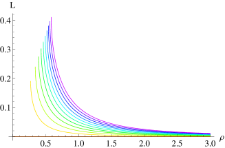
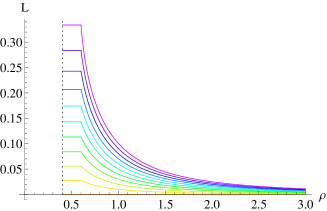
Figure 1: Plots of D7 embeddings in the ${\cal N}=2$ theory. (a) Full embedding solutions for $m=0$. (b) The mebddings interrupted by a two scale cut off.

Numerically we can shoot into the IR from a UV solution with particular values of $c$ and $m$. For the particular case $m=0$ we show such flows in Fig. 1(a). All except the $c=0$ solution appear to stop at some finite $\rho$. In this case we can find the analytic solution to investigate this in more detail. The real solution valid in $\rho\in(\rho_{c},\infty)$, where $\rho_{c}=(2c)^{1/3}$ is

$$L(\rho)=m+{c\over\rho^{2}}{\,}_{2}\mathrm{F}_{1}[1/3,1/2,4/3,4c^{2}/\rho^{6}]$$ (7)

with

$$L^{\prime}(\rho)={2c\over\sqrt{\rho^{6}-4c^{2}}}$$ (8)

From (8) we can see that the gradient of the embedding becomes complex at $\rho_{c}=(2c)^{1/3}$. These results match very well to the numerical results in Fig 1(a) and provide an explicit form for the behaviour at $\rho_{c}$. The only solution that survives to $\rho=0$ is the flow with $c=0$.

One would naively like to plot the effective potential $V(c)$ generated by the holographic flows to show the $c=0$ solution is the minimum. However, since all but one flow (c=0) become ill-defined this is confusing. Understanding why there is no IR effective potential provided by holography is one of our goals. We will adopt the recently suggested idea that we should approach the holographic description in a Wilsonian manner. In particular we will introduce a cut-off in $\rho$, the holographic direction for quark physics (i.e. the radial direction on the D7 brane), which we will call $\epsilon$ and study the theory as a function of changing that cut-off.

Thus specifically to convert the “off-shell” flows, with non-vacuum values of the quark condensate, into kosher flows we will interrupt them with a cut-off at an intermediate value of $\rho$. In the UV we find the Euler Lagrange equation solutions with large $\rho$ asymptotics $c/\rho^{2}$ and solve down to the cut-off. A technical issue arises at this point though. The flows ending on the cut-off do not share the same IR boundary conditions since they meet the cut-off at arbitrary angles. Formally one should not compare their actions in a Euler-Lagrange analysis.

To cure this let us imagine a more general structure for our cut-off in which it has finite width. We introduce two cut-offs in $\rho$, $\epsilon_{-}$ and $\epsilon_{+}$. In the UV from infinite $\rho$ down to $\epsilon_{+}$ we use the flows in Fig 1(a). Then we match these flows to flows beginning at $\epsilon_{-}$ with $L^{\prime}(\epsilon_{-})=0$ and ending at $\epsilon_{+}$ at the same point as the UV flows. We pick this boundary condition at $\epsilon_{-}$ because it naturally matches on to the boundary condition of the regular flows as $\epsilon_{-}\rightarrow 0$ ie $L^{\prime}(0)=0$. We show example flows in Fig 1(b). Now all of our flows have the same IR and UV boundary conditions.

Having introduced this cut-off structure it is actually most natural to remove it by taking $\epsilon_{+}\rightarrow\epsilon_{-}$. In this example the flows between $\epsilon_{-}$ and $\epsilon_{+}$ simply become short straight lines whose action vanishes as the two cut-offs coincide. This digression therefore is just to justify that one can effectively consider the UV flows down to the common $\epsilon$ to share IR boundary conditions and directly compare their action sensibly. In other words we assume a small change to the flows at the cut-off that bends them to satisfy $L^{\prime}(\epsilon)=0$ but assume this doesn’t make a large change to the action. Here this seems rather trivial but we shall see much more structure emerge in the later example with density.

We now proceed in this case with the single cut-off $\epsilon$. For each choice of $\epsilon$ we can plot a potential (density) given by

$$V_{\mathrm{eff}}(c)=-\int_{\epsilon}^{\infty}d\rho\ {\cal L}(\rho)$$ (9)

which is nothing but a Euclidean on-shell action (3) normalized by ${\cal N}$ and a field theory volume (so it is a density.). These actions diverge in the UV but the difference between them determines which is preferred (or they can be regulated by adding a holographic counter term $\sim\Lambda^{4}/4$, where $\Lambda$ is a UV cut-off to be set to $\infty$ at the end). A minus sign comes from Euclideanization. To regulate these flows we will always compute the difference in action from the flat embedding $L=0$ with the equivalent cut-off $\epsilon$. The $L=0$ embedding will therefore always lie at $V=0$ in our plots. The potential should be viewed as the potential energy incurred for a particular value of the condensate from scales above the cut-off $\epsilon$. In other words this potential is the equivalent of the potential in the “bare” Lagrangian written down for the theory at the given cutoff which should be used in conjunction with quantum (or holographic) behaviour below the cut-off. This is exactly the Wilsonian paradigm.

II.1 Wilsonian Potentials

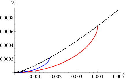
Figure 2: Plots of the effective potential against the parameter $c$ in the ${\cal N}=2$ theory. Plots for $\epsilon=0.2,0.15,0.1$ (red,blue,black) from right to left. The dotted curve is the extended IR effective potential with the values of the action frozen at the point the embeddings become complex.

Using the methodology described above we can now plot the Wilsonian effective potential for the quark condensate as a function of cut off scale $\epsilon$. We show this in Fig 2. Reassuringly $c=0$ is the minimum of the potential at all values of the cut off as we would expect in the supersymmetric theory.

The finite extent of the plots in $c$ is a result of solutions with larger $c$ having gone complex before reaching the cut off at $\epsilon$. We interpret the removal of states with large values of the condensate from the effective potential as a sign that these states can not be reached with the energy available in the IR theory. This seems to match well with a Wilsonian approach and explains the degeneracy if $\epsilon\rightarrow 0$. In the examples below we will simply omit states that are not in the low energy theory in this sense. One could though simply freeze the potential value at the point where the embedding becomes complex and retain that value for lower choices of the cut off. We plot that version of the IR effective potential for the ${\cal N}=2$ system as the dotted curve in Fig 2 - again it is minimized at $c=0$.

III Wilsonian Flow for a Chiral Condensate

We will now move on to study more interesting examples of gauge theories that induce chiral symmetry breaking in the IR. We next look at the ${\cal N}=2$ theory with an applied magnetic field which induces a chiral condensate  Filev:2007gb . We introduce the B field through the D7 brane world volume gauge field in (2). We now have

$${\cal L}=-\rho^{3}\sqrt{(1+L^{\prime 2})}\sqrt{\left(1+\frac{R^{4}}{(L^{2}+\rho^{2})^{2}}B^{2}\right)}\,.$$ (10)

At large $\rho$ the asymptotic solution is again given by (6) and we can again interpret $m,c$ as the quark mass and condensate. In the absence of $B$ the theory is conformal so it is natural to write all dimensionful parameters in units of $\sqrt{B}$, the intrinsic conformal symmetry breaking scale, which we do for our numerical work (i.e. put $B=1$).

The solutions of the Euler-Lagrange equations for the embedding $L(\rho)$ are well known Filev:2007gb ; Evans:2010iy and we show two regular solutions with $m=0$ and with $L^{\prime}(0)=0$ in Fig 3(a) - numerically one shoots out from $\rho=0$ to find these. More generally one can seek such solutions for any mass $m$ and read off the condensate $c$ from the large $\rho$ asymptotics. In Fig 3(b) we show a plot of $c$ vs $m$ for the regular embeddings. It has the spiral structure discussed in Filev:2007gb . The Fig 3(a) solutions are the $c=0$ flat embedding and the largest $c$ solution with $m=0$. The vacuum energy of these configurations can be found by integrating minus the holographic action over the $\rho$ coordinate. These actions diverge in the UV but the difference between them determines which is preferred (or they can be regulated by adding a holographic counter term $\sim\Lambda^{4}/4+B^{2}/2\log\Lambda$, where $\Lambda$ is a UV cut-off to be set $\infty$ at the end). The curving configuration shown, with the quark condensate, is the preferred state and the flat embedding is a local maximum of the effective potential.

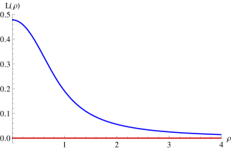
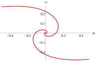
Figure 3: In (a) we show the flat and vacuum embeddings of the D7 brane probe in AdS${}_{5}\times$S⁵ with a magnetic field ($B=1$). In (b) we plot the quark condensate against mass extracted from embeddings such as those in (a).

III.1 Wilsonian Effective Potentials

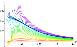
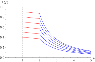
Figure 4: (a) Plots of the D7 embeddings against $\rho$ for several asymptotic values of the quark condensate at zero quark mass with a magnetic field ($B=1$). (b) Those flows interrupted by a two scale cut-off ($\epsilon_{-}=1$ and $\epsilon_{+}=2$ here) used to give the flows the same IR boundary condition.

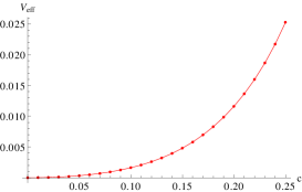
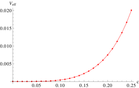
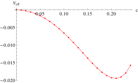
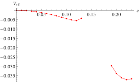
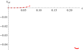
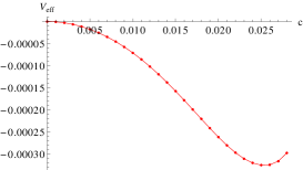
Figure 5: Plots of the Wilsonian effective potential for the quark condensate in the D3/D7 system with a world volume magnetic field ($B=1$) at different values of the Wilsonian cut-off $\epsilon$ ($\epsilon=0.5,0.4686$(phase transition point)$,0.3,0.2,0.15$ and $0.03$ respectively). In (a)-(c) we see a second order transition from the unbroken to the broken phase. In (d)-(e) we see the IR potential degenerate as non-vacuum states are integrated out. In (f) we show the potential close to the origin at $\epsilon=0.03$ displaying one of the metastable vacua, which corresponds to $c\sim 0.025$ also shown in Fig 3(b).

As in the previous example we would like to plot the effective potential $V(c)$ generated by the holographic flows to show the solutions we have found are the turning points. To describe off-shell states we find numerical solutions of the embedding equation for massless quarks that look like $c/\rho^{2}$ at large $\rho$ and shooting into the interior. We plot these flows in Fig 4(a), where it can be seen that most fail to reach the $L$ axis or a deep IR cut-off. We expect that these are associated to the embedding becoming complex by continuity to the $c>>B^{3/2}$ curves, although here we do not have analytic solutions.

To proceed we again introduce a cut off. In Fig 4(b) we show such a cut off with the two scale structure, $\epsilon_{+},\epsilon_{-}$ that allows us to make the flows all share the same $L^{\prime}(\epsilon_{-})=0$ boundary condition. As with the pure supersymmetric case we can take $\epsilon_{-}\rightarrow\epsilon_{+}$ limit trivially here, having a single cut off $\epsilon$ at which we end the flows. We now proceed in this case with the single cut-off $\epsilon$ evaluating the action integrated from $\epsilon$ to infinity.

In Fig 5 we plot the potential as a function of $\epsilon$ for the D3/D7 system with magnetic field. When $\epsilon$ is large we are describing the UV lagrangian which has no preference for a quark condensate. As $\epsilon$ decreases we are “adding in” more of the strongly coupled quantum effects of the theory from lower scales to the bare potential. The first clear feature shown in Fig 5(a)-(c) is that there is a phase transition at the critical value $\epsilon_{c}=0.4686B^{1/2}$ to the chiral symmetry broken phase. This transition is our first main result. One can think of this transition as being in the spirit of a Coleman-Weinberg transition - at high energies the theory has no condensate but then strongly coupled loop effects enter in the IR and break the symmetry. We will return to the deep IR later but let us first explore this phase transition in detail.

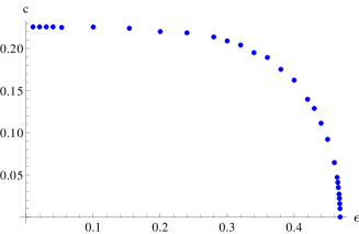
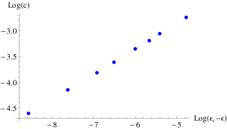
Figure 6: (a) A plot of the quark condenste $c$ against Wilsonian cut-off scale $\epsilon$. (b) A log log plot of the same close to the transition point to show the mean field exponent.

In Fig 6 we plot the quark condensate against $\epsilon$ showing that the transition is second order. We also plot $\log c$ vs $\log(\epsilon_{c}-\epsilon)$ near the transition point from which we can extract the critical exponent as $1/2$ - the transition is a mean field one.

In fact close to the transition we can perform a numerical fit to the potential we have derived of the form

$$V_{\mathrm{eff}}(c;\epsilon,B)=ac^{p}+bc^{q}$$ (11)

where $a$ and $b$ are functions of $\epsilon$ and $B$. Through the range $0.467-0.48$ the fit gives $p=2$ and $q=4$ to better than a percent.

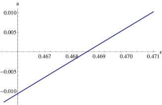
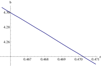
Figure 7: Plots of the parameters (a) $a$ and (b) $b$ in our fitting potential in (11) against Wilsonian cut-off $\epsilon$ through the transition point.

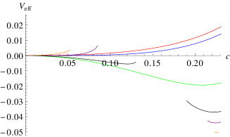
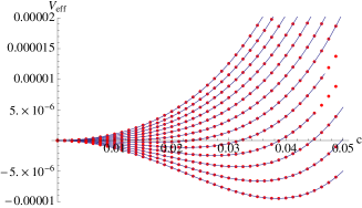
Figure 8: (a) A summary plot of Fig 5 showing the Wilsonian potential at six different choices of $\epsilon$ on a single plot. (b) The potential and fit (solid line) close to the transition point - the dots are holographically determined data.

The existence of such a potential (which is not present in the far UV theory at all) corresponds to the emergence of multi-trace operators in the spirit of the discussion in Heemskerk:2010hk ; Faulkner:2010jy . We next plot the coefficients $a,b$ against $\epsilon$ in Fig 7. $a$ and $b$ are approximated as linear functions close to the transition. $a$ is proportional to $(\epsilon-\epsilon_{c})$ and $b$ is always positive. This is all standard mean field expectations. In Fig 8(a) we plot the potential for different $\epsilon$ on a single plot. In Fig 8(b) we plot the potential for values of $\epsilon$ close to the transition, where the points are the numerical data whilst the solid curves are our fit potentials.

$$\begin{split}V_{\mathrm{eff}}(c;\epsilon,B)&=-4.17\left(0.4686-\frac{\epsilon}{\sqrt{B}}\right)\frac{c^{2}}{B}\\ &\quad+\left(-13.98\frac{\epsilon}{\sqrt{B}}+10.81\right)\frac{c^{4}}{B^{4}}\ .\end{split}$$ (12)

It is clear that the transition is well described by the expected mean field potential. We stress though that here we have derived this form holographically.

Another key feature is visible in Fig 5(d)-(e). When we impose a cut-off at $\rho=\epsilon$ we are excluding some range of condensates. In fact even for large $\epsilon$, flows with very large $c$ become complex in the UV before they reach the cut-off as we saw in the ${\cal N}=2$ supersymmetric theory. Qualitatively it makes sense that if we write a Wilsonian effective model at low energies then large condensate values should be excluded from the theory since such states would be completely integrated out - they have an energy above the cut-off.

As we move to much lower $\epsilon$, the deep IR, in addition some intermediate ranges of condensate also disappear from the effective description in the same fashion. This is why there are breaks in the potential plot for low $\epsilon$. Again qualitatively these states have such high energy relative to the low cut-off scale of the effective theory that they are integrated out.

If $\epsilon$ is strictly taken to zero only the regular flows corresponding to the turning points of the potential have finite action. This is clear from Fig 4(a). The effective potential we are computing therefore degenerates in the deep IR. In this Wilsonian language though this degeneration seems entirely appropriate - when we have integrated out anything above the vacuum energy it is no surprise we are left with only the vacuum state in our effective theory.

In addition to the vacuum state we have considered so far, in principle, at $\epsilon=0$ there are an infinite number of meta-stable vacua near the flat embedding. This is shown in the self-similarity (spiral) structure in the $c$ vs $m$ plot in Fig 3(b). This self-similarity is realized in our Wilsonian context as follows. When $\epsilon$ is large $c=0$ is the global minimum. As $\epsilon$ decreases it becomes a local maximum and a new ground state forms. This is shown in Fig 5(c). As $\epsilon$ decreases more, $c=0$ becomes a local minimum Fig 5(e), which is preparing to produce a new meta-stable vacuum. As $\epsilon$ decreases yet further then $c=0$ becomes a local maximum again Fig 5(f) leaving a meta stable vacuum. This process (from Fig 5(c) to Fig 5(f)) will continue as $\epsilon\rightarrow 0$ leaving more and more meta stable points. The first of these metastable vacua is visible in Fig 5(f) where we have focused near the origin at yet lower $\epsilon$.

Finally here we should comment that the precise meaning of these phase transitions and absent regions will depend on the precise choice of cut-off. The cut-off in $\rho$ seems natural in the D7 context but without a precise link between the holographic direction and the field theory RG scale there is some ambiguity. For example one could have chosen to make the cut-off at constant $r=\sqrt{\rho^{2}+L^{2}}$ surface rather than constant $\rho$. Actually we find that particular choice unnatural because the true IR vacuum state would be missing from the $\epsilon=0$ theory since the chiral symmetry breaking flow does not hit $r=0$. Further at the point where the true vacuum disappears from the IR theory its vacuum energy remains above that of the flat embedding because the flat embedding has a missing contribution to its energy from where it extends below the cut off - we don’t see the true vacuum emerge at any scale. This discussion shows though that the choice of cut-off could be dependent on the explicit flow. Although this identification remains an outstanding problem we believe the Wilsonian style description we have presented is very plausible and qualitatively helpful in understanding the holographic description.

III.2 Towards an on-shell IR effective potential

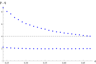
Figure 9: The fitting powers $p,q$ in (11) as a function of Wilsonian cut-off $\epsilon$ below the second order transition.

It is clear from our Wilsonian analysis above that the deep IR effective potential is highly degenerate. It is interesting though to track the form of the effective potential below the Wilsonian second order transition we described above. We can again fit the potential at varying $\epsilon$ to a potential of the form in (11). In Fig 9 we show the best fit values of the powers $a,b$ with $\epsilon$. Although $a$ stays close to 2, $b$ rises fast at values of $\epsilon$ below the second order transition. Of course this does not mean that the $c^{4}$ term is switching off but that the coefficients of $c^{6},c^{8},..$ type terms are becoming large - one could in principle use a more complex potential fitting form to see this behaviour. At lower values of $\epsilon$ than those shown in Fig 9 the potential starts to become degenerate.

In the deep IR ($\epsilon=0$) only the vacuum configuration with $c=0.2255B^{3/2}$ and $V=-0.05534B^{2}$ is described holographically. If one wishes one can imagine (using dimensional analysis) an effective potential of the form

$$V_{\mathrm{eff}}=\alpha\frac{c^{2}}{B}+\beta\frac{c^{4}}{B^{4}}$$ (13)

and fit for $\alpha$ and $\beta$. We find $\alpha=-2.17659$ and $\beta=21.4014$.

It is important to stress though that the form of this potential is not fixed by the holographic flows - we could have included more terms with higher powers of $c$ for example that would reproduce the computed values of $c$ and $V$. Also there is no sense in which this potential is derived away from the minimum - it is an off-shell effective potential extrapolated from on-shell values. That is (13) is assumed to be true for off-shell $c$ values so that the condition $\frac{\partial V}{\partial c}=0$ makes sense. However, $\alpha$ and $\beta$ are fixed only by on-shell data. In our off-shell method at finite $\epsilon$ above, $\alpha$ and $\beta$ are determined by the off-shell data.

The on-shell action also describes a second order phase transition as $B\rightarrow 0$. For $B>0$ the quark condensate grows as $B^{3/2}$ as it must on dimensional grounds. It is important to stress the difference between this transition and the holographic transition we found above with changing $\epsilon$ at fixed B.

III.3 $B$ and perpendicular $E$

The pure B field theory is also very closely related to the theory with both a magnetic and perpendicular electric field present Karch:2007pd ; OBannon:2007in ; Erdmenger:2007bn ; Albash:2007bq . The D7 action is

$${\cal L}=-\rho^{3}\sqrt{(1+L^{\prime 2})}\sqrt{\left(1+\frac{R^{4}}{(L^{2}+\rho^{2})^{2}}(B^{2}-E^{2})\right)}\,,$$ (14)

Clearly this is little different from the previous case since we have an effective $\tilde{B}=\sqrt{B^{2}-E^{2}}$. Indeed one can think of this system as a boosted version of the static case with just a $B$ field. However, we find it a useful case to consider in this form because we can compare the magnitude of the condensate in units of the magnetic field with varying electric field value. It is interesting to have more than one scale in the problem.

One expects, since $\tilde{B}$ is the only scale in the DBI action that at small $E$ values

$$c\sim(B^{2}-E^{2})^{3/4}$$ (15)

In other words there should be a second order transition at $E=B$ with a non-mean field exponent.

Above the transition the theory exhibits a singular surface where the DBI action naively turns complex. This can be resolved by introducing currents induced by the electric field. The theory becomes a conductor as well as chirally symmetric. We will not be exploring this high $E$ phase here.

We can study the theory in our Wilsonian approach with a cut-off $\epsilon$. The theory is equivalent to the analysis of our previous section but with $B$ replaced by $\tilde{B}$. We can write the effective potential, valid close to the Wilsonian transition (12)

$${V_{\mathrm{eff}}\over\tilde{B}^{2}}=\alpha\left(\frac{\epsilon}{\tilde{B}^{1/2}}-\eta\right)\frac{c^{2}}{\tilde{B}^{3}}+b\frac{c^{4}}{\tilde{B}^{6}},$$ (16)

where

$$\eta=\frac{\epsilon_{c}}{\tilde{B}^{1/2}}=0.4686,\quad\alpha=4.17$$ (17)

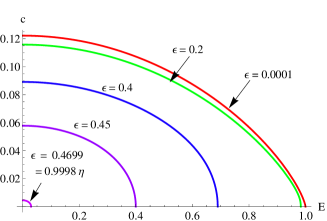
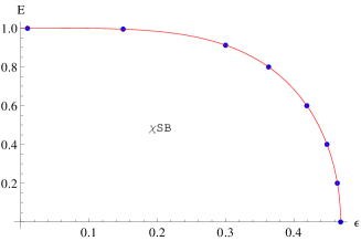
Figure 10: (a) Plot of the quark condensate against electric field (with a background perpendicular $B$ field ($B=1$)) at different values of $\epsilon$. (b) Plot of the $E-\epsilon$ phase diagram - the points are derived from the holographic flows whilst the continuous curve is $E=\sqrt{1-(\epsilon/\eta)^{4}}$

We can now hold $\epsilon$ fixed and vary $E$. This potential tells us the full $E$ dependence of the theory near the transition point. In particular we can determine the transition point from where the mass term changes sign.

$$E_{c}^{2}=B^{2}-\frac{\epsilon^{4}}{\eta^{4}}$$ (18)

Further by writing $E=E_{c}+\delta E$ and expanding we find the effective mass squared depends on $E$ as

$$m^{2}=\frac{\alpha}{2}\frac{\eta^{4}}{\epsilon^{4}}\sqrt{B^{2}-E^{2}}E_{c}(E-E_{c})$$ (19)

In other words the transition is mean field as one moves in $E$ as well as $\epsilon$.

In Fig 10 we plot the condensate against $E$ for various choices of $\epsilon$ and the phase diagram in the $E-\epsilon$ plane. It is important to realize that the transition for which we have found the effective potential is that at finite positive $B^{2}-E^{2}$ and finite $\epsilon$ close to the transition in $\epsilon$. In other words our effective theory describes the $c-E$ plot only near the $c=0$ axis. We can see that the range of validity of our effective theory is only away from the point $\tilde{B}=0$ (i.e. away from $E=B$)

$$\sqrt{B^{2}-\frac{\epsilon^{4}}{\eta^{4}}}<E<B$$ (20)

which clearly has no extent at $\epsilon=0$ The point $\epsilon=0$ on the E axis of the $c-E$ plot is distinct with a critical exponent of $3/4$ relative to the mean-field exponent along the rest of the axis. We can not compute the form of the effective potential for the transition at $\epsilon=0$ other than in the on-shell fashion described in the previous section.

IV Transitions with $B$-field and Density

The next models we will explore are the D3/D7 and the D3/D5 systems with magnetic field, to trigger chiral symmetry breaking, and density, $d$, which opposes chiral symmetry breaking. The phase stucture of these theories has been explored in Evans:2010iy ; Jensen:2010vd for the D3/D7 system that has a second order mean field transtion with increasing density, and in Jensen:2010ga ; Evans:2010hi for the D3/D5 system that displays a holographic BKT transition in which the condensate grows like an exponential of $-1/\sqrt{d_{c}-d}$. Our goal is again to use Wilsonian techniques to learn about these transitions and find the form of the effective potential responsible for the BKT transitions. This system is more complicated than the pure $B$ system as we shall see but we will again enforce that all flows we compare have the same IR boundary conditions at the Wilsonian cut-off to give a concrete prescription. The outcome is a consistent Wilsonian picture of the theories and our ability to derive the effective potential for the condensate including a potential that generates the BKT behaviour. We will concentrate first on the D3/D7 system.

IV.1 Density in the D3/D7 system

Density is introduced into the theory through a background value for the temporal gauge field of the $U(1)$ baryon number Nakamura:2006xk ; Kobayashi:2006sb ; Kim:2006gp ; Kim:2007zm . The UV asymptotic form of the field is $\tilde{A}_{t}=2\pi\alpha^{\prime}A_{t}=\mu+d/\rho^{2}+..$ and describes the chemical potential $\mu$ and the quark density $d$. The probe D7 DBI action with $\tilde{A}_{t}$ is given by

$$\mbox{${\cal L}$}=-\rho^{3}\sqrt{1+L^{\prime 2}-\tilde{A}_{t}^{\prime 2}}\sqrt{1+\frac{B^{2}}{(\rho^{2}+L^{2})^{2}}}$$ (21)

Since the action only depends on the derivative of $\tilde{A}_{t}$ there is a conserved charge density, $d$, defined as

$$d\equiv\frac{\partial\mbox{${\cal L}$}}{\partial\tilde{A}_{t}^{\prime}}\,.$$ (22)

We may Legendre transform the Lagrangian (21) to write the action in terms of density

$$\begin{split}\mbox{${\cal L}$}_{\mathrm{LT}}&=\mbox{${\cal L}$}-\tilde{A}_{t}^{\prime}d\\ &=-\sqrt{1+L^{\prime 2}}\sqrt{d^{2}+\rho^{6}\left(1+\frac{B^{2}}{(\rho^{2}+L^{2})^{2}}\right)}\end{split}$$ (23)

For fixed $B$ and $d$ we can find solutions to the embedding equation of the D7 brane with UV behaviour $m+c/\rho^{2}$. We plot example flows in Fig 11(a). At first sight this system seems rather different from the $d=0$ theory - solutions for a large range of $c$ extended all the way to $\rho=0$. One can naively evaluate the action of these curves and plot it as an effective potential against $c$ - see Fig 11(b). This interpretation is though incorrect for several reasons.

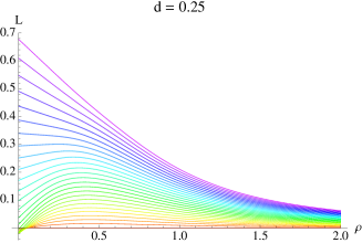
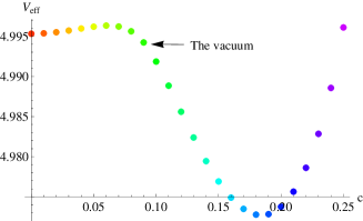
Figure 11: (a) D7 embeddings with a fixed $B$ field ($B=1$) and density ($d=0.25$) but varying condensate $c$. (b) The incorrect effective potential derived by integrating over the action of the flows in (a) - the position of the true vacuum is marked.

Firstly, these flows all meet the $L$ axis at different angles. This means that they have different IR boundary conditions and we should not compare their action in a standard Euler-Lagrange context. Further, since $L^{\prime}(0)\neq 0$ these branes are actually kinked at $\rho=0$, when $SO(4)$ rotated to provide the full D7 embedding.

Secondly, these flows have a non-zero gauge field on their surface that should be sourced. In Kobayashi:2006sb the authors argued that the correct source should be fundamental strings stretched between the D3 (or the origin) and the D7 branes. These would be explicitly the quarks corresponding to the density. Such a continuous distribution of fundamental strings can be absorbed into the D7 world volume and show up as the D7 brane spiking to the origin of the space. The authors of Kobayashi:2006sb argued in this way that only the embedding that ends at the origin was a “good” flow and it should represent the vacuum. This is now the standard interpretation and has provided a coherent picture across a wide range of problems including density.

Note that, with a naive choice of boundary condition shown in Fig 11(a), the vacuum flow for massless quarks is not the minimum of the potential (Fig 11(b)). This is no surprise since the other flows are not physical.

Using the “good” flow condition one can compute the quark condensate against density at fixed $B$ (Fig 12). There is a phase transition at $d=d_{c}=0.3198$. It is second order and mean field in nature ($c\sim\sqrt{d_{c}-d}$).

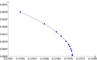
Figure 12: A plot of the quark condensate parameter $c$ versus density in the D3/D7 system with a magnetic field $B=1$.

IV.2 Wilsonian Flows and Potentials

Our traditional analysis of the D3/D7 system with $B,d$ has again left us with no consistent supergravity flows that describe off-shell quark condensate configurations. Let us try to use a Wilsonian cut-off to provide a hint as to how to proceed. To make progress we will again introduce a cut-off with structure consisting of two boundaries in $\rho$ at $\epsilon_{-}$ and $\epsilon_{+}$.

First consider the case when $\epsilon_{-}=0$ but $\epsilon_{+}$ is finite. For massless quarks, we shoot in from the UV, using a boundary condition of the form $c/\rho^{2}$, to the cut-off $\epsilon_{+}$. These configurations must be unified to a single IR boundary condition at $\epsilon_{-}$. They also have a non-zero $A_{t}$ on their world volumes for which we must provide a source. Two of the flows, the true vacuum and the flat $L=0$ embedding, have smooth extensions to $\epsilon_{-}=0$ which end at the origin. These flows describe good vacuum states of the field theory and must be included. They, therefore, dictate what our choice must be for the $\epsilon_{-}$ boundary condition: we must have the flows satisfying $L(\epsilon_{-})=0$, so that we can correctly compare their actions. It is natural then to complete the off shell solutions with flows from $L(\epsilon_{-})=0$ to $\epsilon_{+}$ that meet the UV flows. We show such flows in Fig 13.

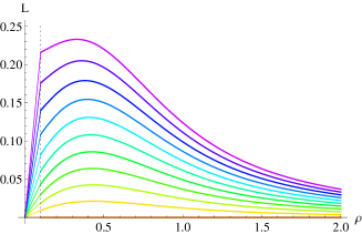
Figure 13: An example of matching UV flows to flows between the two cut-offs $\epsilon_{+}$ and $\epsilon_{-}$ (here $\epsilon_{-}=0$) which have $L(\epsilon_{-}=0)=0$.

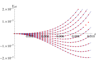
Figure 14: The effective potential with $\epsilon_{-}=0$ and $\epsilon_{+}=0.01$. $B=1$. Every curve is for a fixed density increasing from bottom to top. The red points are computed from the holographic flows, the blue lines are our fit potential.

We can explore the phase transition with changing density at fixed magnetic field using this cut-off prescription for the deep IR. In Fig 14 we show the effective potential for a range of $d$. Here we take $\epsilon_{-}=0$ and $\epsilon_{+}=0.01$ so the cut-off is very thin. There is a second order transition as $d$ is raised matching the previously derived critical value of $d$. Close to the transition point with changing $d$ we can perform a fit to the form of the potential and we find

$$V_{\mathrm{eff}}(c;d)=-5.53(0.3198-d)c^{2}+30.76c^{4}\ ,$$ (24)

This is a mean field potential. In Fig 14 the points are holographically derived data whilst the curves are this fit potential. The coefficients of this mean field potential is a function of $\epsilon_{+}$ in general, but a qualitative mean-field potential form is valid for all $\epsilon_{+}$ near the phase transition.

Now we would again like to shrink $\epsilon_{+}$ to $\epsilon_{-}$ to return to a single cut-off, which will fix our potential uniquely as a function of $\epsilon=\epsilon_{-}=\epsilon_{+}$. If we do that with $\epsilon_{-}=0$ then the UV flows become those we had declared unphysical in Fig 11(a) but with an added length of D7 extending up the $L$ axis from the origin. This suggests that that spike is the completion of the flows to make them physical. One can think of that spike as the fundamental strings that should source the $A_{t}$ gauge field on the D7 world volume.

What then is the correct way to include the spike contribution at non-zero $\epsilon_{-}$? The natural answer seems to be to maintain the condition $L(\epsilon_{-})=0$ at finite $\epsilon_{-}$. We must enforce the same boundary condition on all the flows at $\epsilon_{-}$ and that condition must smoothly map to the case $\epsilon_{-}=0$. When we remove the structured cut-off by taking $\epsilon_{+}\rightarrow\epsilon_{-}\equiv\epsilon$ we will again be left with a spike from the flow of Fig 11(a) to the $\rho$ axis, but now at the scale $\epsilon$ as shown in Fig 15.

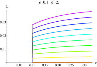
Figure 15: Our prescription for completing the flows of Fig 11(a) at non-zero Wilsonian cut off is to extended them with a spike lying along the cut-off down to the $\rho$ axis as shown.

In a Wilsonian sense we would argue this is reasonable since the UV degrees of freedom should see all the IR physics compressed at the IR cut-off scale $\epsilon$. In some sense the UV theory can not distinguish the origin from the point ($L=0,\rho=\epsilon$). Flows of the form shown in Fig 15 will then be our cut-off prescription away from $\epsilon=0$.

The benefits of this configuration are that with a large cut-off the spike simply increases the action of non-zero $c$ configurations and will leave $c=0$ as the vacuum, whilst in the $\epsilon\rightarrow 0$ limit it will reproduce the known physical solution as the potential minimum. To compute the action of the spike we simply take a very thin limit of our two $\epsilon$ prescription - in particular below we will use $\epsilon_{+}=\epsilon_{-}+0.001$.

Taking this prescription we will now show that we get a sensible Wilsonian story including a derivation of an appropriate effective potential for both the D3/D7 and D3/D5 systems.

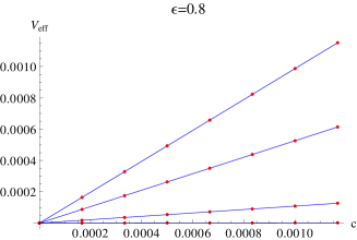
(a) $\epsilon=0.8$. $d=0.001,0.1,0.5,1$ from bottom. The theory is always in the chiral phase.

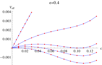
(b) $\epsilon=0.4$. $d=1/300,1/100,1/62$(transition point),$1/30,1/10$ from bottom. There is a first order transition

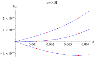
(c) $\epsilon=0.01$. $d=0.3085,0.30879$(transition point),$0.309$. There is a second order transition

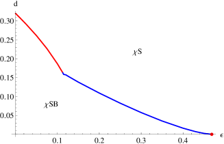
(d) The $d$-$\epsilon$ phase diagram. The blue colour corresponds to a first order transition and the red to second order.

Figure 16: The D3/D7 system $d$-$\epsilon$ phase diagram ($B=1$).

We first present results for the D3/D7 system. In Fig 16(a)-(c) we show the effective potential as a function of $c$ for three choices of $\epsilon$ and various $d$. $B=1$ is fixed. At large $\epsilon$ for all $d$ we see that $c=0$ is the prefered vacuum. As $\epsilon$ is decreased, provided $d<d_{c}\sim 0.32$, there is then a transition to a chiral symmetry broken phase. We show examples of values of the cut-off where this transition is first order and second order in Fig 16(b) and (c) respectively. We can summarize the full picture by drawing the $d-\epsilon$ phase diagram which we show in Fig 16(d). Note that the $d=0$ transition point matches that we found above. The $\epsilon=0$ transition point reproduces our potential fit in (24). The red line is a mean-field second order transition, while the blue lie is a first order transition.

The insertion of the quark spike with $\epsilon$ has therefore provided a believable Wilsonian picture. In fact though as presented so far the IR diverges from the story we told at $d=0$. In particular we argued that the potential should degenerate as $\epsilon\rightarrow 0$ as all states other than the vacuum are integrated from the low energy Wilsonian theory. We simply don’t observe the embeddings that shoot in from the UV becoming complex in this system with density for embeddings with condensate values of order $d$ (very large choices of $c$ do still go complex). We’ve not been able to find a simple resolution. Most likely the effective potential we are deriving here is equivalent to that we produced in the pure ${\cal N}=2$ theory freezing and retaining the potential value at the point where the embeddings go complex - see Fig 2(b). We leave this issue for future thought.

IV.3 BKT transitions in the D3/D5 system

The D3/D5 system with magnetic field and density displays a (holographic) BKT transition Jensen:2010ga . The reason it is distinct from the D3/D7 case is that both $B$ and $d$ are dimension 2 in 2+1 dimension and they can be tuned against each other in the deep IR to force the embedding scalar mode of the theory to violate the Breitenlohner Freedman bound of the effective IR AdS₂. The result is that a BKT transition occurs with an exponential growth of the order parameter (quark condensate) for $d$ below $d_{c}=\sqrt{7}B$ ($c\sim e^{-1/\sqrt{d_{c}-d}}$). This is discussed in detail in Jensen:2010ga ; Evans:2010hi . Our goal here is to derive an effective potential for a BKT transition.

The probe D5 brane is embedded in the $t$ and two $x$ directions of the D3 brane coordinates so that the quarks live on a 2+1 dimensional defect in the ${\cal N}=4$ gauge theory Karch:2000gx ; DeWolfe:2001pq ; Erdmenger:2002ex ; Myers:2008me . The D5 brane also extends in three directions perpendicular to the D3 brane. The probe D5 brane DBI action with $\tilde{A}_{t}$ and $B$ present is given by

$$\mbox{${\cal L}$}=-\rho^{2}\sqrt{1+L^{\prime 2}-\tilde{A}_{t}^{\prime 2}}\sqrt{1+\frac{B^{2}}{(\rho^{2}+L^{2})^{2}}}$$ (25)

We may Legendre transform to write the action in terms of density (22)

$$\begin{split}\mbox{${\cal L}$}_{\mathrm{LT}}&=\mbox{${\cal L}$}-\tilde{A}_{t}^{\prime}d\\ &=-\sqrt{1+L^{\prime 2}}\sqrt{d^{2}+\rho^{4}\left(1+\frac{B^{2}}{(\rho^{2}+L^{2})^{2}}\right)}\,.\end{split}$$ (26)

For fixed $B$ and $d$ we can find solutions to the embedding equation of the D7 brane with UV behaviour $m+c/\rho$.

Following the last section we will introduce a cut-off at the scale $\epsilon$ and complete the UV flows with a spike down the cut-off to the $\rho$ axis (we again fix $\epsilon_{+}=\epsilon_{-}+0.001$ to generate the spike’s action) - see Fig 15. We can determine the phase diagram of the theory in the $d-\epsilon$ space at fixed $B$ which is shown in Fig 17. The transition is first order at large $\epsilon$ (the blue line) then becomes a mean field second order transition at small $\epsilon$ before finally ending on a BKT transition at $\epsilon=0$. The cut-off behaves like temperature which has already been observed to convert the BKT transitions to second order with the introduction of any non-zero temperature Jensen:2010ga ; Evans:2010hi .

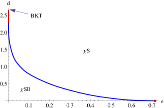
Figure 17: The D3/D5 system $d$-$\epsilon$ phase diagram ($B=1$). The blue colour corresponds to a first order transition, the red to a second order and the end point BKT transition is labelled.

We plot the $\epsilon\rightarrow 0$ potential for varying choices of $d$ in Fig 18. This potential can not be well fitted by a mean field potential. Instead if we fit to

$$V_{\mathrm{eff}}=ac^{2}+bc^{2}(\log c)^{2}$$ (27)

we find a good fit - see Fig 18. The fitting potential in Fig 18 is

$$V_{\mathrm{eff}}(c;d)=(0.74d^{2}-4.72)c^{2}+(0.016d^{2}-0.12)c^{2}(\log c)^{2}$$ (28)

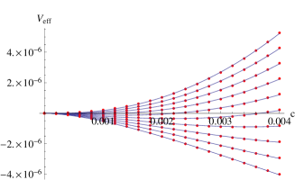
Figure 18: The potential with the cut-off $\epsilon=0$ for the condensate in the D3/D5 system at fixed $B$ ($B=1$) and finite density close to the transition. Every curve is for a fixed density increasing from bottom to top. Red points are holographic data and the blue curves are the fitted potential in (28).

This potential form implies that the condensate near the phase transition is

$$c\sim e^{-\frac{\sqrt{-4a+b}}{2\sqrt{b}}}\sim e^{\frac{-3.29}{\sqrt{2.77-d}}}\ .$$ (29)

Note that to numerically extract this data one needs to work at extremely high accuracy near the transition where the condensate is exponentially small. The data shown are the best we have managed. In fact the form of the condensate is known analytically to be given by  Jensen:2010ga ; Evans:2010hi

$$c\sim e^{\frac{-3.86}{\sqrt{2.65-d}}}$$ (30)

Although we have not reproduced this perfectly our numerics support this form. We consider it a considerable success to have derived the potential for the BKT transition in the holographic setting.

V Conclusions

We have analyzed the phase structure of a number of theories that break chiral symmetry and have a holographic dual using a Wilsonian cut-off. Including a cut-off allows us to consider off-shell states, i.e. configurations with a value of the quark condensate different from that in the true vacuum. We believe that the results give an improved intuitive understanding of the holographic description and we have been able to derive low energy effective actions for the phase transitions in these models including a potential for a BKT transition. The precise identification of our cut-offs in the holographic description and the equivalent cut-off structure in the gauge theory remains inexact but the spirit seems correct.

We first studied the D3/D7 system (the ${\cal N}=4$ gauge theory with quark hypermultiplets in 3+1d). This theory has ${\cal N}=2$ supersymmetry and does not generate a quark condensate. We nevertheless can in principle plot an effective potential for the condensate that should be minimized at zero. The D7 embedding encodes the quark condensate and in Fig 1(a) we display the Euler Lagrange solutions for the theory with different condensate values. In Fig 1(b) we insert a cut-off at a finite value of $\rho$ - here we give the cut-off some finite width and use that width to match all of the solutions to solutions of the Euler Lagrange equations with the same IR boundary condition at the lower cut-off. In this case as one shrinks the width of the cut-off, the UV action returns to that of just the UV flow. In Fig 2 we plot the Wilsonian potential, evaluated from the action of the D7 brane above the cut-off, in the theory as a function of cut-off value. The Wilsonian potential is indeed minimized at zero condensate at all energy scales. There is a finite extent of the potential in the quark condensate because the embeddings become complex (which we showed analytically in (7). We interpret the removal of large condensate configurations from the low energy effective actions as representing those configurations having too high energy to appear in the low energy theory.

The same system with an applied magnetic field has chiral symmetry breaking. We display the Euler Lagrange solutions for the D7 branes with different condensate values in Fig 4(a). We introduced a cut off at finite $\rho$ as in the pure ${\cal N}=2$ theory. In Fig 5 we plot the resulting Wilsonian potential as a function of cut-off value. The UV of the theory preserves chiral symmetry. The system then shows a second order mean field transition to the broken phase at intermediate cut-offs in the spirit of a Coleman Weinberg transition. The form of the potential near the transition can be extracted numerically and is displayed in (12). Finally in the deep IR non-vacuum configurations begin to be integrated out of the IR effective theory because they can not be accessed with the IR theory’s energy and the effective potential again degenerates.

We translated these results to the theory with a magnetic field and perpendicular electric field. This theory shares the same DBI action as the pure B theory but our results enlarge to describe the phase diagram in the electric field versus cut-off plane, which we show in Fig 10.

We then added a constant quark density into the D3/D7 theory with magnetic field. The density opposes chiral symmetry breaking. In Fig 11 we show the D7 embeddings for different values of the quark condensate which are again ill determined because they end at the IR axis in a kinked configuration. The true vacuum is the embedding that ends at the origin. Introducing a cut-off with width as in Fig 13 allows us to define non-vacuum configurations that all end at the origin. If we take that cut-off to zero then the embeddings are completed by a spike to the origin. For a generic value of the Wilsonian cut-off we have suggested that such a spike should be introduced along the cut-off as shown in Fig 15. Using this prescription we have determined the phase structure in the density, cut-off plane at fixed magnetic field, see Fig 16. Here we see first order transitions with changing Wilsonian scale as well as mean field cases. The IR transitions are mean field and the effective potential is of the form given in (24) (in units of $B$).

Finally we looked at the D3/D5 system describing the ${\cal N}=4$, 3+1 dimensional theory with quarks introduced on a 2+1 dimensional defect. Here with a magnetic field and density the zero temperature theory exhibits a holographic BKT transition. We have again determined the phase diagram in the density cut-off plane at fixed magnetic field in Fig 17. As the cut-off is lowered the transition changes from first to second order before becoming a BKT transition in the deep IR. We have been able to derive an effective potential for the BKT transition in the IR given by (28).

The Wilsonian style analysis therefore allows one to see strongly coupled versions of Coleman Weinberg like symmetry breaking transitions. It also allows us to derive the low energy effective action in these theories by defining off-shell configurations. The effective potential for the BKT transition is a new result derived here.

A number of problems remain to be analyzed in these settings including introducing finite temperature and looking at the non-mean field transitions that lie between mean field and BKT transitions Evans:2010np . We hope to study these in the future. These methods will hopefully also be of use away from the probe limit where even simple deformations of AdS are typically singular and hard to interpret Girardello:1999bd ; Gubser:2000nd .

- (1) I. Bredberg, C. Keeler, V. Lysov, and A. Strominger, Wilsonian Approach to Fluid/Gravity Duality, JHEP 1103 (2011) 141, [arXiv:1006.1902].
- (2) D. Nickel and D. T. Son, Deconstructing holographic liquids, arXiv:1009.3094.
- (3) I. Heemskerk and J. Polchinski, Holographic and Wilsonian Renormalization Groups, JHEPA,1106,031.2011 1106 (2011) 031, [arXiv:1010.1264].
- (4) T. Faulkner, H. Liu, and M. Rangamani, Integrating out geometry: Holographic Wilsonian RG and the membrane paradigm, arXiv:1010.4036.
- (5) M. R. Douglas, L. Mazzucato, and S. S. Razamat, Holographic dual of free field theory, Phys.Rev. D83 (2011) 071701, [arXiv:1011.4926].
- (6) S.-J. Sin and Y. Zhou, Holographic Wilsonian RG Flow and Sliding Membrane Paradigm, JHEP 1105 (2011) 030, [arXiv:1102.4477]. * Temporary entry *.
- (7) S.-S. Lee, Holographic description of quantum field theory, Nucl.Phys. B832 (2010) 567–585, [arXiv:0912.5223].
- (8) S.-S. Lee, Holographic description of large N gauge theory, Nucl.Phys. B851 (2011) 143–160, [arXiv:1011.1474].
- (9) E. T. Akhmedov, A Remark on the AdS / CFT correspondence and the renormalization group flow, Phys.Lett. B442 (1998) 152–158, [hep-th/9806217].
- (10) E. T. Akhmedov, Notes on multitrace operators and holographic renormalization group, hep-th/0202055.
- (11) J. de Boer, E. P. Verlinde, and H. L. Verlinde, On the holographic renormalization group, JHEP 0008 (2000) 003, [hep-th/9912012].
- (12) J. de Boer, The Holographic renormalization group, Fortsch.Phys. 49 (2001) 339–358, [hep-th/0101026].
- (13) A. Lewandowski, M. J. May, and R. Sundrum, Running with the radius in RS1, Phys.Rev. D67 (2003) 024036, [hep-th/0209050].
- (14) A. Lewandowski, The Wilsonian renormalization group in Randall-Sundrum 1, Phys.Rev. D71 (2005) 024006, [hep-th/0409192].
- (15) J. M. Maldacena, The Large N limit of superconformal field theories and supergravity, Adv.Theor.Math.Phys. 2 (1998) 231–252, [hep-th/9711200].
- (16) L. Susskind and E. Witten, The Holographic bound in anti-de Sitter space, hep-th/9805114.
- (17) A. W. Peet and J. Polchinski, UV / IR relations in AdS dynamics, Phys.Rev. D59 (1999) 065011, [hep-th/9809022].
- (18) N. Evans, T. R. Morris, and O. J. Rosten, Gauge invariant regularization in the AdS/CFT correspondence and ghost D-branes, Phys.Lett. B635 (2006) 148–150, [hep-th/0601114].
- (19) A. Karch and E. Katz, Adding flavor to AdS/CFT, JHEP 06 (2002) 043, [hep-th/0205236].
- (20) J. Erdmenger, N. Evans, I. Kirsch, and E. Threlfall, Mesons in Gauge/Gravity Duals - A Review, Eur. Phys. J. A35 (2008) 81–133, [arXiv:0711.4467].
- (21) J. Babington, J. Erdmenger, N. J. Evans, Z. Guralnik, and I. Kirsch, Chiral symmetry breaking and pions in non-supersymmetric gauge / gravity duals, Phys. Rev. D69 (2004) 066007, [hep-th/0306018].
- (22) S. Nakamura, Y. Seo, S.-J. Sin, and K. P. Yogendran, A new phase at finite quark density from AdS/CFT, J. Korean Phys. Soc. 52 (2008) 1734–1739, [hep-th/0611021].
- (23) S. Kobayashi, D. Mateos, S. Matsuura, R. C. Myers, and R. M. Thomson, Holographic phase transitions at finite baryon density, JHEP 02 (2007) 016, [hep-th/0611099].
- (24) V. G. Filev, C. V. Johnson, R. C. Rashkov, and K. S. Viswanathan, Flavoured large N gauge theory in an external magnetic field, JHEP 10 (2007) 019, [hep-th/0701001].
- (25) A. Karch and A. O’Bannon, Metallic AdS/CFT, JHEP 09 (2007) 024, [arXiv:0705.3870].
- (26) N. Evans, A. Gebauer, K.-Y. Kim, and M. Magou, Holographic Description of the Phase Diagram of a Chiral Symmetry Breaking Gauge Theory, JHEP 03 (2010) 132, [arXiv:1002.1885].
- (27) K. Jensen, A. Karch, and E. G. Thompson, A Holographic Quantum Critical Point at Finite Magnetic Field and Finite Density, JHEP 05 (2010) 015, [arXiv:1002.2447].
- (28) N. Evans, A. Gebauer, and K.-Y. Kim, Phase Structure of the D3/D7 Holographic Dual, JHEP 05 (2011) 067, [arXiv:1103.5627].
- (29) N. Evans, K. Jensen, and K.-Y. Kim, Non Mean-Field Quantum Critical Points from Holography, Phys. Rev. D82 (2010) 105012, [arXiv:1008.1889].
- (30) N. Evans, T. Kalaydzhyan, K.-y. Kim, and I. Kirsch, Non-equilibrium physics at a holographic chiral phase transition, JHEP 01 (2011) 050, [arXiv:1011.2519].
- (31) N. Evans, J. French, and K.-y. Kim, Holography of a Composite Inflaton, JHEP 11 (2010) 145, [arXiv:1009.5678].
- (32) A. Karch and L. Randall, Open and closed string interpretation of SUSY CFT’s on branes with boundaries, JHEP 06 (2001) 063, [hep-th/0105132].
- (33) O. DeWolfe, D. Z. Freedman, and H. Ooguri, Holography and defect conformal field theories, Phys. Rev. D66 (2002) 025009, [hep-th/0111135].
- (34) J. Erdmenger, Z. Guralnik, and I. Kirsch, Four-Dimensional Superconformal Theories with Interacting Boundaries or Defects, Phys. Rev. D66 (2002) 025020, [hep-th/0203020].
- (35) R. C. Myers and M. C. Wapler, Transport Properties of Holographic Defects, JHEP 0812 (2008) 115, [arXiv:0811.0480].
- (36) K. Jensen, A. Karch, D. T. Son, and E. G. Thompson, Holographic Berezinskii-Kosterlitz-Thouless Transitions, Phys. Rev. Lett. 105 (2010) 041601, [arXiv:1002.3159].
- (37) N. Evans, A. Gebauer, K.-Y. Kim, and M. Magou, Phase diagram of the D3/D5 system in a magnetic field and a BKT transition, Phys. Lett. B698 (2011) 91–95, [arXiv:1003.2694].
- (38) S. R. Coleman and E. J. Weinberg, Radiative Corrections as the Origin of Spontaneous Symmetry Breaking, Phys.Rev. D7 (1973) 1888–1910.
- (39) A. O’Bannon, Hall Conductivity of Flavor Fields from AdS/CFT, Phys. Rev. D76 (2007) 086007, [arXiv:0708.1994].
- (40) K.-Y. Kim, J. P. Shock, and J. Tarrio, The open string membrane paradigm with external electromagnetic fields, arXiv:1103.4581.
- (41) N. Evans, K.-Y. Kim, and J. P. Shock, Chiral phase transitions and quantum critical points of the D3/D7(D5) system with mutually perpendicular E and B fields at finite temperature and density, arXiv:1107.5053. * Temporary entry *.
- (42) J. Erdmenger, R. Meyer, and J. P. Shock, AdS/CFT with Flavour in Electric and Magnetic Kalb-Ramond Fields, JHEP 12 (2007) 091, [arXiv:0709.1551].
- (43) T. Albash, V. G. Filev, C. V. Johnson, and A. Kundu, Quarks in an External Electric Field in Finite Temperature Large N Gauge Theory, JHEP 08 (2008) 092, [arXiv:0709.1554].
- (44) K.-Y. Kim, S.-J. Sin, and I. Zahed, Dense hadronic matter in holographic QCD, hep-th/0608046.
- (45) K.-Y. Kim, S.-J. Sin, and I. Zahed, The Chiral Model of Sakai-Sugimoto at Finite Baryon Density, JHEP 01 (2008) 002, [arXiv:0708.1469].
- (46) L. Girardello, M. Petrini, M. Porrati, and A. Zaffaroni, The supergravity dual of N = 1 super Yang-Mills theory, Nucl. Phys. B569 (2000) 451–469, [hep-th/9909047].
- (47) S. S. Gubser, Curvature singularities: The Good, the bad, and the naked, Adv.Theor.Math.Phys. 4 (2000) 679–745, [hep-th/0002160].