Detailed Chemical Abundances of Four Stars in the Unusual Globular Cluster, Palomar 1

Abstract

Detailed chemical abundances for twenty one elements are presented for four red giants in the anomalous outer halo globular cluster Palomar 1 ($R_{\rm{GC}}=17.2$ kpc, $Z=3.6$ kpc) using high-resolution ($R=36000$) spectra from the High Dispersion Spectrograph (HDS) on the Subaru Telescope. Pal 1 has long been considered unusual because of its low surface brightness, sparse red giant branch, young age, and its possible association with two extragalactic streams of stars—this paper shows that its chemistry further confirms its unusual nature. The mean metallicity of the four stars, $[\rm{Fe/H}]=-0.60\pm 0.01$, is high for a globular cluster so far from the Galactic center, but is low for a typical open cluster. The [$\alpha$/Fe] ratios, though in agreement with the Galactic stars within the $1\sigma$ errors, agree best with the lower values in dwarf galaxies. No signs of the Na/O anticorrelation are detected in Pal 1, though Na appears to be marginally high in all four stars. Pal 1’s neutron capture elements are also unusual: its high [Ba/Y] ratio agrees best with dwarf galaxies, implying an excess of second-peak over first-peak s-process elements, while its [Eu/$\alpha$] and [Ba/Eu] ratios show that Pal 1’s contributions from the r-process must have differed in some way from normal Galactic stars. Therefore, Pal 1 is chemically unusual, as well in its other properties. Pal 1 shares some of its unusual abundance characteristics with the young clusters associated with the Sagittarius dwarf galaxy remnant and the intermediate-age LMC clusters, and could be chemically associated with the Canis Majoris overdensity; however it does not seem to be similar to the Monoceros/Galactic Anticenter Stellar Stream.

1. Introduction

Ever since its discovery by Abell (1955), Palomar 1 (Pal 1) has been tentatively classified as a globular cluster (GC), primarily because of its location high above the Galactic plane ($Z=3.6$ kpc; Harris 1996, 2010 edition). However, Pal 1 has several anomalous characteristics that have cast doubt upon this classification. For example, Pal 1 appears to be unusually young for an outer halo GC. Using standard isochrone fits to Pal 1’s ground-based color-magnitude diagram (CMD), Rosenberg et al. (1998a) estimated an age between $6.3$ and $8$ Gyr, while Sarajedini et al. (2007) found an age between 4 and 6 Gyr with HST photometry. This F606W ($\sim$V), F814W ($\sim$I) HST CMD of the central field of Pal 1 from Sarajedini et al. 2007 (see Figure 1) shows the main sequence turn-off around F606W $\approx 19.4$ ($V\approx 19.6$), and a possible detection of a red horizontal branch near F606W $\approx 16.4$ ($V\approx 16.6$). Thus, $\Delta V^{\rm{HB}}_{\rm{MSTO}}\approx 3$, making the cluster younger than about 7 Gyr (with the method of Chaboyer et al. 1996). These estimates make Pal 1 one of the youngest GCs, along with Ter 7, Pal 12, and Whiting 1, whose ages range from $7-9$ Gyr (e.g. Buonanno et al. 1998; Salaris & Weiss 2002; Carraro et al. 2007; Dotter et al. 2010).

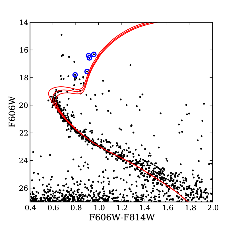
Figure 1.— An HST color-magnitude diagram (roughly V, V-I) for the central field of Pal 1 from Sarajedini et al. (2007). The observed targets are circled. Also shown are fitted isochrones from the Dartmouth Stellar Evolution Database (Dotter et al., 2008) for ages of 4, 5, and 6 Gyr. Values of $[\rm{Fe/H}]=-0.6$, $[\alpha/\rm{Fe}]=0.0$, $(m-M)_{V}=16.27$, and $E(B-V)=0.20$ are adopted, as discussed in the text

Pal 1 also lacks luminous, evolved stars. The CMD in Figure 1 shows a sparsely populated red giant branch and a barely detectable horizontal branch. Furthermore, near-infrared medium-resolution spectroscopy of the Ca II triplet (CaT) lines in four of these red giants has shown that Pal 1 is fairly metal-rich for an outer halo GC, with an average $[\rm{Fe/H}]=-0.6$ (on the Zinn-West scale, using the standard Galactic CaT line strength to metallicity conversion; Rosenberg et al. 1998b). The main sequence is also poorly populated, and therefore the entire cluster has an extremely low total luminosity for a GC ($M_{V}=-2.52$; Harris 1996, 2010 edition).

Clearly Pal 1 does not conform to the characteristics of traditional Galactic GCs, suggesting either that Pal 1 is not a GC or that it is not Galactic. If Pal 1 has been misclassified as a GC, another possibility is that it could be an open cluster (OC)—this option seems unlikely due to the combination of its position above the Galactic plane, its high concentration parameter ($c=2.57$; Harris 1996, 2010 edition), and its age (although Pal 1’s age is comparable to that of the oldest known OCs, e.g. VandenBerg & Stetson 2004). However, Pal 1’s brightness and age place it in greater agreement with the OCs than with the GCs (see Figure 3 in Carretta et al. 2010). The ambiguity surrounding the OC vs. GC classification leads to a need for a more rigorous distinction between the two. From observations of many Galactic GCs, Carretta et al. (2010) defined a GC as a cluster that shows signs of a second generation of stars through a Na/O anticorrelation. Under this definition, if Pal 1 does not show signs of a Na/O anticorrelation, then it cannot be considered a classical GC.

Alternatively, Pal 1 could have originated in a dwarf galaxy and been accreted by the Milky Way during a merger. The latter situation is plausible, as several other Galactic GCs, notably the young clusters listed above, have been linked to dwarf galaxies. M54, Arp 2, Ter 7, and Ter 8 lie on a stream associated with the Sagittarius dwarf spheroidal (Sgr dSph) galaxy (Da Costa & Armandroff, 1995); Pal 12 has been kinematically linked to the Sgr dSph through proper motion studies (Dinescu et al., 2000); Whiting 1 is undergoing tidal stripping and appears to lie in a stream of M giants from the Sgr dSph (Carraro et al., 2007); and Rup 106 has been tentatively associated with the Magellanic Clouds because of its location along the Magellanic stream (Lin & Richer, 1992). Pal 1 does appear to lie along several stellar streams that may be extragalactic but have not yet been associated with any galaxies. One such stream, known both as the Monoceros stream and as the Galactic Anticenter Stellar Stream (GASS), appears to be from a disrupted dwarf satellite (e.g. Sollima et al. 2011); Pal 1’s position, velocity, and metallicity make it a possible member of this stream (Crane et al., 2003). The Canis Major overdensity, which seems to be distinct from the GASS (Chou et al., 2010b), has also been associated with Pal 1, again because of the cluster’s coincidental location (Martin et al., 2004). Finally, Pal 1 has also been tentatively linked to the “Orphan Stream” (Belokurov et al., 2007), though its radial velocity and metallicity make it an unlikely member (Newberg et al., 2010). Though no obvious association with a particular stream has been confirmed, tidal tails around Pal 1 have recently been discovered, suggesting that the cluster itself is being dissipated in the tidal field of the Galaxy (Niederste-Ostholt et al., 2010).

In the absence of an obvious host galaxy, detailed chemical abundances can be used to examine if Pal 1 has an extragalactic origin. It has been well established (e.g. Tolstoy et al. 2009, Venn et al. 2004) that metal-rich stars in Local Group dwarf galaxies have distinctly different chemical abundances from stars in the Milky Way, at a given metallicity (the differences are not so obvious by $[\rm{Fe/H}]\sim-2$). These chemical variations between the environments are due to different star formation histories and efficiencies, which are linked to the mass of the galaxy and the properties of its environment. Therefore, the differences are not just between dwarf galaxies and normal galaxies—in fact, dwarf galaxies have unique chemical evolutions, meaning that it is possible to chemically link a star to its host galaxy (e.g. Tolstoy et al. 2009, Freeman & Bland-Hawthorn 2002). These chemical differences are not just seen in field stars, they are also seen in GCs; for example, Pritzl et al. (2005) showed that most Galactic GCs have similar chemical abundances to Galactic field stars at the same metallicity, with Pal 12, Ter 7, and Rup 106 as notable exceptions.

Detailed, high-resolution chemical abundances have been used to trace the origin of several globular clusters. In particular Pal 12 (Cohen, 2004) and Ter 7 (Tautvais̆ienė et al. 2004, Sbordone et al. 2005b) have [$\alpha$/Fe] ratios that follow the Sgr dSph field star abundance trends and are clearly separated from Galactic field stars, supporting the hypothesis that they were captured from the Sgr dSph. The more metal-poor Sgr clusters Arp 2 and Ter 8, however, are not chemically distinct from the Galaxy (Mottini et al., 2008), which shows that the [$\alpha$/Fe] deviation can be metallicity- (and presumably age-) dependent. If Pal 1 has an extragalactic origin, then its metallicity of $[\rm{Fe/H}]\approx-0.6$ puts it in a regime where [$\alpha$/Fe] and other chemical abundance ratios should be useful in determining its origin.

Here we present a detailed analysis of high-resolution spectra for four red giant stars in Pal 1, taken with the Subaru Telescope. Monaco et al. (2010) have completed a chemical analysis of one star in Pal 1 (Pal 1-I), also with spectra taken at Subaru, but with independent observations; they find that their single star shows similar abundance patterns to Galactic open clusters. Saviane et al. (2010) further show that its chemistry implies that Pal 1 could be associated with the Canis Major overdensity. With four stars, our analysis allows us to determine the chemical abundance ratios with higher precision, and investigate any star-to-star variations in the abundances that could be linked with chemical or cluster evolution effects. Section 2 outlines the observations and the data reduction, while Section 3 examines our method for measuring equivalent widths. In Section 4 we discuss the model atmospheres, particularly how the atmospheric parameters are derived. Section 5 presents the methods for element abundance determinations, while Section 6 examines the significance of these results with respect to Galactic stars and clusters. Finally, Section 7 examines the origins of Pal 1.

2. Observations and Data Reduction

Four of our target stars are the same stars observed by Rosenberg et al. (1998b): bright, red giant branch (RGB) stars, with radial velocities that make them likely cluster members. We refer to these stars as Pal 1-I, -II, -III, and -IV, following the naming convention of Rosenberg et al. The bright object located at the center of the cluster, Pal 1-C, was also included as a target, although the membership of this object is not as certain as the others. The locations of these stars on a CMD and in an image of the cluster (from Sarajedini et al. 2007) are shown in Figures 1 and 2. In addition to the Pal 1 stars we include an analysis of a “standard” star, M67-141 (as identified by Fagerholm 1906). This star resides in the metal-rich open cluster M67, and has previous detailed, high resolution chemical abundances from Yong et al. (2005) and Pancino et al. (2010). Table 1 shows the positions and magnitudes of the target stars. The Pal 1 positions and V and I magnitudes (in the Johnson system) are from Sarajedini et al. (2007), while M67-141’s position and V and I magnitudes (in the Kron-Cousins system) are from Høg et al. (2000), Sanders (1977), and Janes & Smith (1984), respectively. All of the K magnitudes are from the Two Micron All-Sky Survey (2MASS) Point Source Catalog.

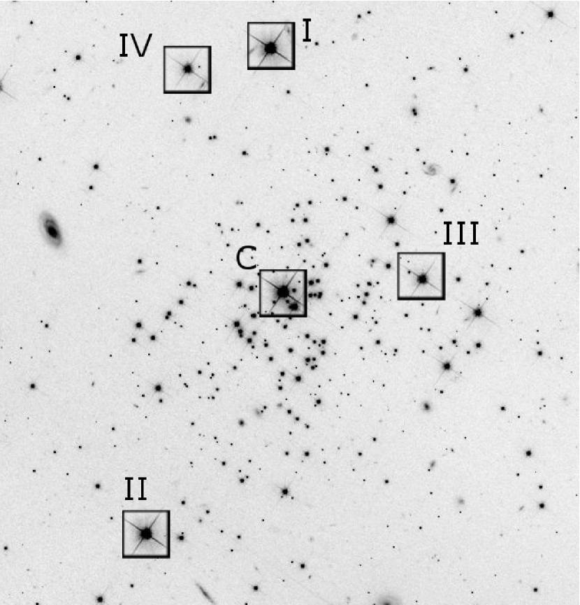
Figure 2.— An HST F814W image of Pal 1, with our targets shown in squares. The field of view is approximately $1.\arcmin 7\times 1.\arcmin 7$. North is up, and west is to the left. Note that we do not perform a full analysis of Pal 1-IV due to poor sky conditions.

Table 1Our target stars, their positions, and their magnitudes

Star	RA (J2000)	Dec (J2000)	V	I	K	References
M67-141	$8^{\rm{h}}51^{\rm{m}}22.8^{\rm{s}}$	$+11^{\circ}48\arcmin 1.\arcsec 7$	10.480	9.400	7.942	1, 2, 3
Pal 1-I	$3^{\rm{h}}33^{\rm{m}}21.8^{\rm{s}}$	$+79^{\circ}35\arcmin 16.\arcsec 2$	16.675	15.459	13.832	4
Pal 1-II	$3^{\rm{h}}33^{\rm{m}}29.6^{\rm{s}}$	$+79^{\circ}34\arcmin 16.\arcsec 2$	16.843	15.618	13.983	4
Pal 1-III	$3^{\rm{h}}33^{\rm{m}}12.3^{\rm{s}}$	$+79^{\circ}34\arcmin 59.\arcsec 2$	17.827	16.628	15.281	4
Pal 1-IV	$3^{\rm{h}}33^{\rm{m}}27.0^{\rm{s}}$	$+79^{\circ}35\arcmin 34.\arcsec 9$	18.032	16.969	15.779	4
Pal 1-C	$3^{\rm{h}}33^{\rm{m}}21.0^{\rm{s}}$	$+79^{\circ}34\arcmin 57.\arcsec 1$	16.603	15.328	13.715	4

These stars were observed on several runs in 2006 January and 2007 January using the High Dispersion Spectrograph (HDS; Noguchi et al. 2002) on the 8.2 m Subaru Telescope. The default grating was centered at 5500 Å  with a slit length of 5.6 arcsec for all stars and a slit width of 1 arcsec for the Pal 1 stars and 0.6 arcsec for M67-141, leading to spectral resolutions of $R=36000$ and $R=60000$, respectively. Table 2 shows a list of the dates, total exposure times, and signal-to-noise ratios (SNR) for these observations. We note that the position of the Moon was not preferable for observations of the Pal 1 stars, as the primary target of this observing run was the Sextans dwarf galaxy (Aoki et al., 2009).

The data were reduced using the basic Subaru HDS pipeline, with standard IRAF routines to remove the bias and flat field, and with additional cosmic ray removal. The stars were fairly low in the sky during the observations and the seeing conditions were poor, meaning the stars observed in 2006 nearly filled the slit; as a result the sky subtractions proved to be extremely difficult. Ultimately some of the star signals were removed along with the sky even when using the outermost 3-pixels on either side of the projected slit spectrum; thus, the final, co-added stellar spectra from 2006 (stars Pal 1-I and -II) have lower SNR than expected. The sky subtraction for one of the 2007 stars, Pal 1-IV, proved impossible, and that star has therefore been dropped from further abundance analyses. The other two stars, Pal 1-III and -C, have good sky subtraction and therefore higher SNR.

The radial velocities were determined by locating several strong, easily-identified spectral lines and calculating the shift in wavelength using Gaussian fits to the lines. These radial velocities were then shifted to heliocentric velocities using the IRAF task rvcorrect; the final heliocentric velocities are listed in Table 2. Though a sky subtraction could not be performed on Pal 1-IV, a radial velocity could still be obtained; this radial velocity is quite different from the other stars, as will be discussed in Section 7.1.3.

Table 2Dates of observations, total exposure times, signal-to-noise ratios at two wavelengths, and calculated heliocentric radial velocities

Star	Dates	Exposure Time (s)	SNR (5310 Å)	SNR (6616 Å)	$v_{\rm{helio}}$ (km s-1)
M67-141	2006 Jan 21	5985	100	150	$+33.9\pm 1.0$
Pal 1-I	2006 Jan 20, 21	9000	15	30	$-77.2\pm 1.0$
Pal 1-II	2006 Jan 20	9000	15	30	$-78.0\pm 1.0$
Pal 1-III	2007 Jan 25, 26	12600	31	45	$-77.2\pm 1.0$
Pal 1-IV	2007 Jan 27, 28, 29	21600	-	-	$-68.1\pm 1.0$
Pal 1-C	2007 Jan 6, 27	5400	35	55	$-77.0\pm 1.0$

The shifted rest-frame spectra were then continuum-normalized. The continuum was estimated using an iterative, non-parametric filter (e.g. Battaglia et al. 2008) designed to split the spectrum into continuum and line components based on a user-defined scale length for allowed continuum variations. This was set at 10 Å  so that the strongest spectral absorption lines were not affected. Figure 3 shows red and blue portions of the final stellar spectra which have a full coverage of approximately 4350 to 7140 Å; the representative spectra in Figure 3 have been arbitrarily shifted vertically for easier comparison.

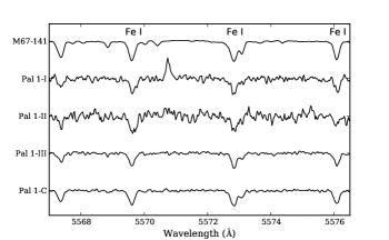
(a) Blue Region

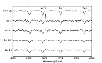
(b) Red Region

Figure 3.— Portions of the five spectra, in both a blue and a red region, with notable spectral lines labelled. The spectra have been continuum normalized and were arbitrarily shifted vertically for the ease of comparison. Note the low S/N of Pal 1-I and -II compared to the other Pal 1 stars.

3. Equivalent Widths

The measured spectral lines are from the line list by Shetrone et al. (2003), with supplemental lines from Cayrel et al. (2004), Aoki et al. (2007), Cohen et al. (2008), Letarte et al. (2009), Tafelmeyer et al. (2010), and Frebel et al. (2010). The equivalent widths (EWs) were fit with Gaussian profiles using splot in IRAF and were checked by numerical interpretation under the continuum. EWs can now be measured with automatic line-measuring programs such as DAOSPEC, a program that is intended for high resolution ($R>15000$), high SNR ($>30$) spectra (Stetson & Pancino, 2008). Some advantages of DAOSPEC over IRAF’s splot include a fixed full-width at half maximum (FWHM) for all lines, and an effective continuum that takes weak features into account; however, it appears that with low SNR spectra DAOSPEC can have difficulty fitting the continuum. Due to the poor quality of the Pal 1-I and -II spectra, IRAF splot measurements are therefore preferred. By a visual comparison with the higher SNR spectra (Pal 1-III and -C), the spectral lines in Pal 1-I and -II were identified and distinguished from noise in the low SNR spectra. Spectral lines in the noisy spectra that had a drastic difference in width or depth from Pal 1-III or -C were discarded.

Table 3The line list.

Wavelength	Element	E.P.	log gf	Equivalent width (mÅ)
(Å)		(eV)		Sun	M67-141	Pal 1-I	Pal 1-II	Pal 1-III	Pal 1-C
4443.19	Fe I	2.86	-1.043	134.0	171.0	-	-	-	-
4476.02	Fe I	2.85	-0.819	-	-	-	-	-	157.0
4484.22	Fe I	3.60	-0.864	100.0	122.0	-	-	76.0	117.0
4489.75	Fe I	0.12	-3.899	91.0	-	-	-	120.0	-
4592.66	Fe I	1.56	-2.462	99.0	185.0	-	-	-	-

Measurements were made relative to the local continuum. For all stars, lines stronger than 200 mÅ  were rejected. For Fe, the Pal 1 lines with EWs stronger than 150 mÅ  were also thrown out, in order to best constrain the atmospheric parameters (discussed in Section 4). The wavelengths (in Å), excitation potentials (in eV), $\log gf$ values, and equivalent widths (in mÅ) for the four Pal 1 stars and the standard star are shown in Table 3.

3.1. IRAF splot vs. DAOSPEC measurements

DAOSPEC has been used for spectral line measurements by several different authors (e.g. Letarte et al. 2010); therefore we compare our splot EWs to those from DAOSPEC. Figure 4 shows a comparison between splot EWs (from this work) and DAOSPEC EWs (from Pancino et al. 2010) for the standard star, M67-141, which has the highest resolution and SNR. Their EW errors from DAOSPEC are also shown. The majority of the offsets between the splot and the DAOSPEC measurements are within our adopted EW measurement errors (shown as dashed lines; see Section 5.3 for a description of how these errors are calculated), and are therefore not significant. The few lines outside these errors are weak lines that we measure to be slightly stronger than DAOSPEC measures—this difference may be attributed to continuum placement (see Stetson & Pancino 2008 for a discussion of their effective continuum). For the weak lines ($>60$ mÅ), the average discrepancy between the two analyses (shown as a dotted blue line) is $4\pm 6$ mÅ.

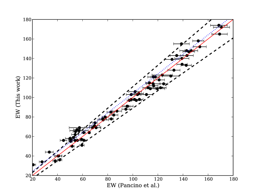
Figure 4.— A comparison of the EWs as measured with splot in IRAF to those measured by the program DAOSPEC (from Pancino et al. 2010) for the standard star M67-141. The red line shows equal EW measurements. The blue dotted line shows the average offset between the weak lines in the two data sets. The dashed lines show the EW errors ($\rm{EW}_{\rm{min}}+10\%\;\rm{EW}$) as calculated using the Cayrel (1988) formula (see Section 5.3).

3.2. A Comparison with Previous Studies

Our EW measurements from the low SNR Pal 1-I spectrum can be compared to those from Monaco et al. (2010). Unfortunately there are very few lines in common for us to compare, due to differences in the spectral range and SNR . For the lines in common, Figure 5 shows our splot EWs versus the Monaco et al. DAOSPEC EWs from the higher SNR spectrum. Also shown are the line of perfect agreement (solid red line), our estimated 1$\sigma$ EW errors (black dashed lines; see Section 5.3), and the average trend (dotted blue line). Our EWs tend to be slightly higher, with an average offset of $7\pm 6$ mÅ. However, the majority of the points in Figure 5 lie within the dashed lines, which implies that the EW measurement techniques and spectral reduction methods are in reasonable agreement. We further note that there does not seem to be a significant trend in error with EW.

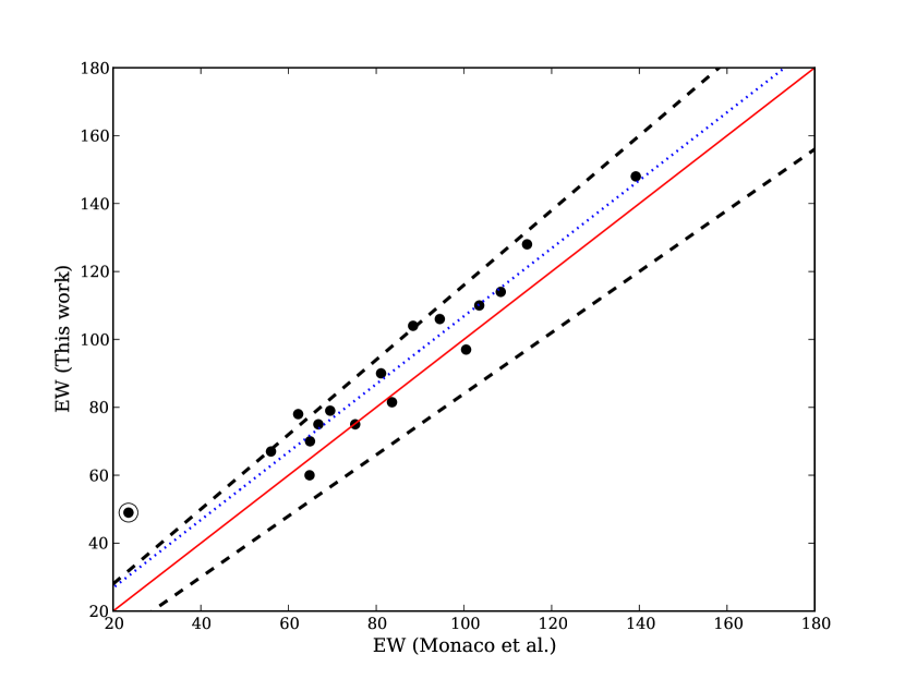
Figure 5.— A comparison between our EWs for Pal 1-I, and those measured by Monaco et al. (2010), for the lines in common between our analyses. EW errors were not given in Monaco et al. (2010). The circled point is a Cr I line that is unusally discrepant; for that reason we have removed it from the analysis. The dashed lines represent the EW errors, as discussed in Section 5.3. The blue dotted line shows the average offset between the two data sets. Note that though we tend to measure slightly larger EWs, the differences are typically less than the EW errors.

4. Model Atmospheres

Stellar atmospheric parameters (effective temperature, $T_{\rm{eff}}$; surface gravity in its logarithmic form, $\log g$; microturbulence, $\xi$, in km s^-1; and metallicity, [Fe I/H]) are initially derived from broadband photometry and revised based on spectral indicators as described below.

4.1. Photometric Parameters

Determining the atmospheric parameters from broadband colors requires knowledge of the metallicity, reddening, distance modulus, and mass of the stars. The initial metallicity for M67-141, $[\rm{Fe/H}]=0.01$, comes from Yong et al. (2005), while the initial metallicity for the Pal 1 stars, $[\rm{Fe/H}]=-0.6$, comes from the CaT measurements of Rosenberg et al. (1998b). The surface temperatures are estimated using the colors of the stars (from the magnitudes shown in Table 1). The $(V-K)$ color to temperature conversion of Alonso et al. (1999, with the correction) is used—this conversion is based on a large sample of Galactic GCs and field stars and is calibrated in the TCS photometric system. Conversions from $(V-K)_{\rm{Johnson}}$ to $(V-K)_{\rm{TCS}}$ are therefore used (Alonso et al., 1998).

The Alonso et al. (1999) calibrations are based on the absolute colors of the stars, meaning the cluster reddening must be taken into account. The adopted reddenings for Pal 1 and M67-141 are $E(B-V)=0.20\pm 0.03$ and $E(B-V)=0.033\pm 0.005$, from the Schlegel et al. (1998) dust extinction maps. The $E(V-K)$ reddening is determined with the conversions of McCall (2004). The final photometric temperatures are shown in Table 4.

The bolometric correction for each star is calculated using the formula from Alonso et al. (1999), and the absolute bolometric magnitude is determined using the distance modulus. For M67-141 we simply adopt the absolute distance modulus quoted in Yong et al. (2005): $(m-M)_{0}=9.56$. For Pal 1 there are two different literature values for the distance modulus: Rosenberg et al. (1998a) give (m-M)${}_{0}=15.25\pm 0.25$ while Sarajedini et al. (2007) give (m-M)${}_{0}=15.65\pm 0.10$. Both are determined through main sequence fitting of Pal 1 to the lower main sequence of 47 Tuc, a Galactic globular cluster with a similar metallicity to Pal 1. We adopt the Sarajedini et al. (2007) distance modulus, (m-M)${}_{V}=16.26$, which is determined from HST photometry.

Finally, the photometric surface gravity is determined through a luminosity comparison with the Sun, which requires knowledge of the mass of our stars. All the targets are evolved stars: M67-141 is in the red clump (Yong et al., 2005) and the Pal 1 stars are all presumably on the RGB. If we assume that there has been minimal mass loss since the stars evolved off the main sequence, and if we assume that not much time has passed since the stars left the main sequence, then the main sequence turn off mass can be used as the RGB stellar mass. For most Galactic GCs this turnoff mass is typically $0.8$ M_☉—however, as discussed earlier, both M67 (an open cluster) and Pal 1 are younger than the typical GC, and should therefore have a higher turnoff mass than $0.8$ M_☉. To determine the turnoff mass, we examined the Pal 1 isochrones computed by Sarajedini et al. (2007); an age of $5\pm 1$ Gyr gives a turnoff mass of $M_{\rm{TO}}=1.14\pm 0.06$ M_☉. This estimate agrees with that from Cohen (2004) for Pal 12, another young globular cluster. M67-141 has an age from 4-5 Gyr from isochrone fits (VandenBerg & Stetson, 2004), which means the turnoff mass will be similar. The final photometric gravities are also shown in Table 4.

Table 4Atmospheric Parameters for the Pal 1 stars and the standard star, M67-141.

	Photometric	Spectroscopic
Star	$T_{\rm{eff}}$ (K)	$T_{\rm{eff}}$ (K)	$\log g$	$\xi$ (km s-1)	[Fe/H]	$v\sin i$ (km s-1)
M67-141: This paper	$4624\pm 12$	$4750\pm 50$	$2.31\pm 0.06$	$1.4\pm 0.1$	$0.02\pm 0.02$	4.5
Yong et al. (2005)	4700 (4604)	4700	2.3	1.34	0.00	-
Pancino et al. (2010)	4590	4650	2.8	1.3	0.06	-
Monaco et al: Pal 1-I	4850	5000	2.40	1.0	-0.5	-
Pal 1-I	$4742\pm 81$	$4800\pm 70$	$2.27\pm 0.15$	$1.4\pm 0.3$	$-0.61\pm 0.08$	2.5
Pal 1-II	$4725\pm 80$	$4750\pm 135$	$2.33\pm 0.15$	$1.6\pm 0.2$	$-0.61\pm 0.08$	2.5
Pal 1-III	$5061\pm 90$	$5050\pm 50$	$2.89\pm 0.15$	$0.9\pm 0.1$	$-0.60\pm 0.02$	0.5
Pal 1-C	$4698\pm 79$	$4750\pm 70$	$2.22\pm 0.15$	$1.3\pm 0.1$	$-0.58\pm 0.03$	1.5

4.2. Spectroscopic Parameters

Spectroscopic indicators are examined to refine these photometric parameters. The abundances of the individual Fe lines are analyzed in MOOG (Sneden, 1973), using LTE OSMARCS model atmospheres with spherical geometries (Gustafsson et al. 2008, Plez & Lambert 2002). The final temperature was found by forcing the Fe I line abundances to be independent of the excitation potential ($\chi$); similarly, the microturbulence was refined by forcing the Fe I abundances to be independent of the line equivalent width. The associated errors in these parameters were found using the $1\sigma$ errors of the slopes of the Fe I abundances versus $\chi$ and EW.

It is not clear whether spectroscopic methods are appropriate for determining the gravity (i.e. ensuring that the Fe I and Fe II abundances are equal), since Fe I is expected to suffer from non-LTE effects which depopulate this under represented species through interactions with the radiation field. In addition, there are few Fe II lines in our spectral range; those that are available are located at blue wavelengths so that reliable Fe II abundance determinations can be difficult, especially in low SNR spectra. For these reasons, we choose to adopt the photometric surface gravities and their associated errors.

The final metallicity is the average Fe I abundance, with an error determined from the line-to-line scatter, $\sigma(\textrm{{Fe~{}I}})$, divided by the square root of the number of lines ($\delta(\textrm{{Fe~{}I}})=\sigma(\textrm{{Fe~{}I}})/\sqrt{N}$; see Section 5.3.2). The final spectroscopic values ($T_{\rm{eff}}$, $\log g$, $\xi$, and [Fe/H]) for M67-141 and the Pal 1 stars are listed in Table 4. The spectroscopic and photometric temperatures are in excellent agreement. We also list the atmospheric parameters from the literature for M67-141 (from Yong et al. 2005 and Pancino et al. 2010) and for Pal 1-I (from Monaco et al. 2010). Our values for M67-141 are in excellent agreement with Yong et al. (2005), but our temperature and gravity disagree with Pancino et al. (2010). Our Pal 1-I temperatures are slightly lower and our microturbulence values are slightly higher than Monaco et al. (2010). The differences are primarily due to differing atomic data; as we explain in Section 5.6.2, these atmospheric parameter differences result in slightly different abundances in the various analyses.

Figure 6 shows the abundances from the thirty Fe I lines that were measured in Pal 1-I, generated using the final spectroscopic atmospheric parameters. Note that though there is little to no trend in abundance for excitation potential, reduced equivalent width, or wavelength, there is still a range of $\sim 0.2$ dex.

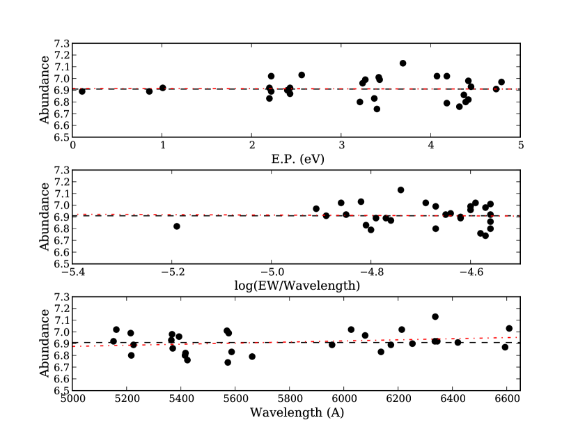
Figure 6.— The abundance trends with excitation potential (top), reduced EW (middle) and wavelength (bottom) for Pal 1-I, with the spectroscopic atmospheric parameters listed in Table 4. The black dashed line shows a constant trend, while the red dot-dashed line shows the trends of the data; note that in all three panels the trend is essentially constant, though there is still a significant dispersion.

5. Elemental Abundances

The elemental abundances were determined in MOOG using EW matching. With these abundances, the logarithmic ratios with respect to Solar values, [X/Fe], are calculated. Tables 5 and 6 show the [X/Fe] ratios, the statistical errors (see Section 5.3 for a description of how these errors are determined), the number of lines used to determine the abundances, and comparisons with literature values. These results will be discussed in Section 6.

Table 5A comparison of the derived abundances in the standard star, M67-141 from this work, Yong et al. (2005), and Pancino et al. (2010). We also give the total error in [X/Fe] and the number of lines used in the calculation.

	Pancino et al. (2010)		Yong et al. (2005)		This work
X	[X/Fe]	$\delta$	[X/Fe]	$\delta$	[X/Fe]	$\delta$	N
Fe I	0.06	0.01	-0.01	0.12	0.02	0.02	91
Fe II	0.01	0.03	0.01	0.09	-0.03	0.04	24
O I	-0.05	0.09	0.10	0.06	-0.15 (0.03)	0.09	2
Na I	0.10	0.02	0.24	0.10	0.29	0.13	4
Mg I	0.29	0.03	0.18	0.04	0.04	0.07	3
Al I	0.06	0.06	0.16	0.06	0.14	0.15	2
Si I	0.09	0.02	0.11	0.08	0.13	0.05	10
Ca I	-0.13	0.02	0.09	0.03	0.07	0.06	15
Sc II	-0.02	0.08	-	-	0.09	0.06	12
Ti I	-0.07	0.02	0.05	0.05	0.02	0.05	35
Ti II	-0.07	0.02	-	-	0.10	0.05	33
V I	0.13	0.04	-	-	-0.05	0.05	17
Cr I	0.01	0.03	-	-	-0.04	0.09	8
Cr II	-	-	-	-	0.18	0.18	2
Mn I	-	-	-0.20	0.03	-0.08	0.13	4
Co I	0.11	0.02	0.01	0.09	-0.15	0.21	2
Ni I	0.06	0.05	0.06	0.09	0.08	0.04	26
Cu I	-	-	-	-	0.16	0.13	3
Zn I	-	-	-	-	0.05	0.12	3
Y II	-0.04	0.02	-	-	-0.04	0.11	5
Ba II	0.26	0.05	0.02	-	0.0	0.17	2
La II	0.06	0.05	0.13	0.04	0.04	0.06	4
Nd II	0.01	0.29	-	-	0.04	0.08	5
Eu II	-	-	0.05	-	0.0	0.12	1

Table 6[X/Fe] ratios, $1\delta$ errors, and the number of lines used, for the Pal 1 stars. The [X/Fe] ratios from Monaco et al. (2010) are also shown for comparison.

	Monaco Pal 1-I	Pal 1-I			Pal 1-II			Pal 1-III			Pal 1-C
X	[X/Fe]	[X/Fe]	$\delta$	$N$	[X/Fe]	$\delta$	$N$	[X/Fe]	$\delta$	$N$	[X/Fe]	$\delta$	$N$
Fe I	-0.49	-0.61	0.08	30	-0.61	0.08	21	-0.60	0.03	81	-0.58	0.03	60
Fe II	-0.53	-0.46	0.30	1	-0.64	0.44	2	-0.61	0.05	23	-0.68	0.05	23
O I	-	$<0.82$	-	1	$<0.32$	-	1	$<0.42$	-	1	0.20 (0.23)	0.11	2
Na I	0.38	0.26	0.34	2	0.23	0.31	2	0.20	0.09	4	0.16	0.09	4
Mg I	0.11	-0.11	0.20	1	-0.13	0.30	1	-0.02	0.08	5	0.02	0.07	6
Al I	0.25	-	-	-	-	-	-	0.0	0.10	2	0.07	0.10	2
Si I	-0.01	0.24	0.24	1	0.13	0.23	1	0.09	0.06	8	0.19	0.06	8
Ca I	0.04	0.16	0.16	6	-0.04	0.22	4	0.15	0.06	17	0.12	0.06	18
Sc II	-0.01	0.28	0.26	3	0.21	0.33	2	0.30	0.09	8	0.21	0.07	12
Ti I	0.10	-0.03	0.34	3	-0.14	0.38	4	0.02	0.06	24	-0.08	0.06	24
Ti II	-	-	-	-	-0.13	0.51	2	-0.08	0.05	32	0.08	0.07	23
V I	-0.06	-0.05	0.21	1	0.08	0.14	4	0.14	0.07	6	0.06	0.05	14
Cr I	-0.23	-	-	-	-	-	-	0.01	0.09	11	-0.16	0.11	9
Cr II	-	-	-	-	-	-	-	0.17	0.20	2	0.19	0.21	2
Mn I	-0.22	-	-	-	-0.16	0.36	1	-0.21	0.12	4	-0.11	0.10	8
Co I	-0.06	-	-	-	-	-	-	-0.10	0.18	2	0.03	0.20	2
Ni I	-0.03	0.05	0.25	3	0.09	0.14	5	0.08	0.05	20	0.03	0.05	21
Cu I	-	-	-	-	-0.05	0.33	1	0.04	0.18	2	-0.08	0.32	1
Zn I	0.38	-	-	-	-	-	-	0.08	0.14	3	0.15	0.15	3
Y II	-0.32	$<0.04$	-	1	$<0.34$	-	1	-0.45	0.12	4	-0.36	0.12	5
Ba II	0.24	0.27	0.24	2	0.19	0.26	2	0.22	0.12	3	0.26	0.18	2
La II	0.29	$<0.38$	-	1	$<0.78$	-	1	0.42	0.16	1	0.24	0.14	3
Nd II	-	0.19	0.65	1	-	-	-	0.13	0.16	2	0.12	0.14	2
Eu II	-	$<0.78$	-	1	$<0.78$	-	1	0.50	0.20	1	0.50	0.20	1

5.1. Hyperfine Structure

The elements Sc, V, Mn, Co, Cu, Ba, La, and Eu were checked for hyperfine structure (HFS) corrections. The majority of the HFS and isotopic data comes from Prochaska et al. (2000, for Sc, V, Mn, and Co), Booth et al. (1983, additional Mn), Biehl (1976, Cu), McWilliam (1998, Ba), and Lawler et al. (2001a, b, La and Eu), with extra lines added from the Kurucz database. The corrections per line were averaged over the entire star and were applied to the average abundances from MOOG. If HFS data were not available, then the line was neglected in the correction calculation. When the corrections were less than 0.1 dex they were ignored. Negligible corrections were found ($<0.1$ dex) for Sc, Ba, La, and Eu; moderate corrections ($\lesssim 0.5$ dex) for V and Mn; and large corrections ($\lesssim 1.0$ dex) for Co and Cu.

5.2. Spectrum Synthesis

When there was only a single absorption line for an important element, a spectrum synthesis was performed on the line. In each spectrum synthesis the instrumental and rotational broadening are taken into account. With resolutions of $R=36000$ and $R=60000$, Pal 1 and M67-141 have instrumental broadening values of 8.3 and 5.0 km s^-1, respectively. The rotational broadenings for each star were determined by examining nearby lines with known abundances, and adjusting the $v\sin i$ values until the widths and depths matched the points. For example, in the case of the the Eu II 6643 Å  line, the 6644 Å  Ni I line and the 6647 Å  Fe I line were used to determine these parameters. The derived $v\sin i$ values for M67-141 and the four Pal 1 stars are shown in Table 4. The abundances were then estimated from the best fits to the adopted models, with an error in $\log\epsilon$ equal to the range of abundances that fit the line profiles. Where the spectral lines were particularly noisy, only upper limits are provided. Spectrum syntheses were also used when a known blend affected an important line, as in the case of the 6141.73 Å  Ba II line, which is blended with a Ni I line at solar metallicity (Allende Prieto et al., 2001). By using a spectrum synthesis the strength of the Ni line could also be taken into account.

An example of a spectrum synthesis of the Mg I 5528 Å  line in Pal 1-I is shown in Figure 7. Note that the width of the line is fit well, but the bottom point is missed; we suspect that this bottom point is a noise spike.

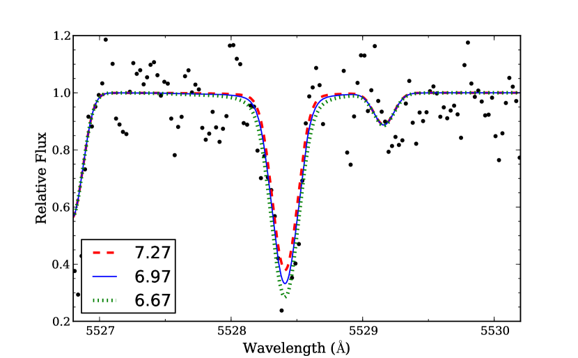
Figure 7.— Spectrum synthesis for the Mg I 5528 Å  line in Pal 1-I Syntheses for three different Mg abundances are shown: $\log\epsilon(\rm{Mg})=7.27$, $6.97$, and $6.67$. The parameters for the synthesis are discussed in Section 5.2. Note that though the fits match the width of the line well, the bottom-most point is not fit; this point is most likely a noise spike.

5.3. Errors

To determine the errors on the abundances, we separate systematic errors (due to model atmosphere parameters) from statistical errors (due to measurements). While the systematic errors are calculated and discussed, they are not included in the errors bars in our figures and are tabulated only in Tables 7 and 8.

5.3.1 Systematic Errors

The abundances from individual spectral lines in a star are all affected by the choice of model atmosphere parameters. Changing each parameter ($T_{\rm{eff}}$, $\log g$, $\xi$, [M/H]) will affect the average abundance of each species. While the errors in the atmospheric parameters themselves are random, changes in these parameters will systematically affect the abundance analyses.

To determine how the abundances were affected by uncertainties in the atmospheric parameters, new model atmospheres were tested by varying one parameter at a time by its $1\sigma$ error. These are quoted individually in Tables 7 and 8. It is not clear how to combine these errors, since they are not independent, e.g. increasing $\log g$ affects the $T_{\rm{eff}}$ and $\xi$ estimates in our analysis. However, investigating their effects separately provides a maximum uncertainty estimate. We also consider systematic errors due to continuum placement; as discussed in Section 3, continuum placement can result in EW differences that are outside our adopted $1\sigma$ errors. As a conservative estimate of these errors, we adopt the average offset between our EW measurements and those of Pancino et al. (2010, 4 mÅ, for the high SNR stars) and Monaco et al. (2010, 7 mÅ, for the low SNR stars), for our continuum uncertainty.

Representative systematic errors in abundances for M67-141, Pal 1-I, and Pal 1-III are shown in Tables 7 and 8, individually and added in quadrature. The differences are largest for the continuum and temperature errors in M67-141, while the errors are fairly similar for all parameters in the Pal 1 stars. The final errors in the [X/Fe] ratios are fairly small for all elements.

Table 7Errors in M67-141’s [X/Fe] ratios due to atmospheric parameter errors. The total error shows the individual errors added in quadrature.

	$\Delta T=+50$ K	$\Delta\log g=+0.06$	$\Delta\xi=+0.1$ km s-1	$\Delta[\rm{M/H}]=+0.02$	Continuum +4 mÅ	Total
$\Delta$[Fe I/H]	+0.07	+0.01	-0.05	+0.01	+0.07	0.11
$\Delta$[Fe II/H]	-0.07	+0.03	-0.05	+0.01	+0.09	0.13
$\Delta$[O I/Fe]	-0.06	+0.02	+0.05	0.0	+0.02	0.08
$\Delta$[Na I/Fe]	+0.01	-0.01	+0.02	-0.01	-0.01	0.03
$\Delta$[Mg I/Fe]	-0.03	0.0	+0.04	0.0	0.0	0.05
$\Delta$[Al I/Fe]	0.0	-0.01	+0.03	-0.01	-0.01	0.03
$\Delta$[Si I/Fe]	-0.10	0.0	+0.03	-0.01	0.0	0.10
$\Delta$[Ca I/Fe]	+0.04	-0.01	0.0	-0.01	-0.01	0.04
$\Delta$[Sc II/Fe]	-0.08	+0.01	0.0	0.0	0.0	0.08
$\Delta$[Ti I/Fe]	+0.09	-0.01	-0.01	-0.01	0.0	0.09
$\Delta$[Ti II/Fe]	-0.08	+0.02	-0.01	0.0	+0.02	0.09
$\Delta$[V I/Fe]	+0.11	0.0	+0.01	0.0	+0.01	0.11
$\Delta$[Cr I/Fe]	+0.08	-0.01	-0.02	-0.01	0.01	0.08
$\Delta$[Cr II/Fe]	-0.13	+0.01	-0.01	-0.01	+0.02	0.13
$\Delta$[Mn I/Fe]	+0.05	0.0	-0.02	0.0	0.0	0.05
$\Delta$[Co I/Fe]	0.0	0.0	-0.02	-0.01	+0.01	0.02
$\Delta$[Ni I/Fe]	-0.03	0.0	0.0	-0.01	0.0	0.03
$\Delta$[Cu I/Fe]	0.0	-0.01	-0.01	0.0	-0.02	0.02
$\Delta$[Zn I/Fe]	-0.11	+0.01	0.0	0.0	+0.03	0.11
$\Delta$[Y II/Fe]	-0.07	+0.02	-0.02	0.0	+0.03	0.08
$\Delta$[Ba II/Fe]	-0.04	+0.02	-0.03	+0.01	0.0	0.05
$\Delta$[La II/Fe]	-0.05	+0.02	+0.04	0.0	+0.02	0.07
$\Delta$[Nd II/Fe]	-0.06	+0.02	+0.02	0.0	+0.05	0.08
$\Delta$[Eu II/Fe]	-0.08	+0.02	+0.04	0.0	+0.02	0.09

Table 8Errors in Pal 1-I and -III’s [X/Fe] ratios due to the atmospheric parameter errors. The total error shows the individual errors added in quadrature.

	$\Delta T_{\rm{eff}}$ (K)		$\Delta\log g$		$\Delta\xi$ (km s-1)		$\Delta$ [M/H]		Continuum (mÅ)		Total
	I	III	I	III	I	III	I	III	I	III	I	III
	$+70$	$+50$	$+0.15$	$+0.15$	$+0.3$	$+0.1$	$+0.08$	$+0.02$	$+7$	$+4$
$\Delta$[Fe I/H]	+0.07	+0.05	0.0	-0.01	-0.18	-0.04	+0.01	0.0	+0.12	+0.08	0.23	0.10
$\Delta$[Fe II/H]	-0.04	-0.03	+0.05	+0.06	-0.08	-0.04	+0.02	0.0	+0.11	+0.14	0.15	0.16
$\Delta$[O I/Fe]	-	-0.04	-	+0.08	-	+0.04	-	+0.01	-	+0.14	-	0.17
$\Delta$[Na I/Fe]	-0.01	-0.02	-0.02	-0.01	+0.08	+0.02	-0.01	0.0	-0.01	-0.03	0.08	0.04
$\Delta$[Mg I/Fe]	-0.02	-0.02	-0.05	-0.02	+0.08	+0.03	0.0	0.0	-0.06	-0.02	0.11	0.05
$\Delta$[Al I/Fe]	-	-0.02	-	+0.01	-	+0.04	-	0.01	-	+0.03	-	0.05
$\Delta$[Si I/Fe]	-0.08	-0.04	+0.02	+0.03	+0.12	+0.04	0.0	+0.01	-0.01	+0.02	0.15	0.07
$\Delta$[Ca I/Fe]	0.0	0.0	-0.02	-0.02	+0.03	+0.01	-0.01	0.0	-0.02	-0.04	0.04	0.05
$\Delta$[Sc II/Fe]	-0.08	-0.05	+0.06	+0.07	+0.09	0.0	+0.01	0.0	+0.01	+0.05	0.14	0.10
$\Delta$[Ti I/Fe]	+0.04	+0.02	+0.01	+0.01	0.0	0.0	-0.01	0.0	+0.04	+0.02	0.06	0.03
$\Delta$[Ti II/Fe]	-	-0.05	-	+0.06	-	0.0	-	0.0	-	+0.05	-	0.09
$\Delta$[V I/Fe]	+0.05	+0.02	0.0	+0.02	+0.14	+0.03	-0.01	0.0	0.0	+0.03	0.15	0.05
$\Delta$[Cr I/Fe]	-	+0.02	-	-0.01	-	-0.01	-	0.0	-	-0.01	-	0.03
$\Delta$[Cr II/Fe]	-	-0.07	-	+0.07	-	0.0	-	+0.01	-	+0.07	-	0.12
$\Delta$[Mn I/Fe]	-	+0.01	-	-0.01	-	0.0	-	+0.01	-	-0.02	-	0.03
$\Delta$[Co I/Fe]	-	0.0	-	+0.03	-	+0.02	-	+0.01	-	+0.04	-	0.05
$\Delta$[Ni I/Fe]	-0.01	-0.02	+0.02	+0.01	+0.01	0.0	-0.01	0.0	+0.01	+0.01	0.03	0.02
$\Delta$[Cu I/Fe]	-	0.0	-	+0.01	-	-0.02	-	0.0	-	+0.01	-	0.02
$\Delta$[Zn I/Fe]	-	-0.07	-	+0.04	-	0.0	-	0.0	-	+0.05	-	0.09
$\Delta$[Y II/Fe]	-	-0.05	-	+0.07	-	0.0	-	+0.01	-	+0.08	-	0.12
$\Delta$[Ba II/Fe]	-0.05	-0.04	+0.05	+0.04	-0.08	-0.02	+0.02	+0.01	0.0	-0.01	0.11	0.06
$\Delta$[La II/Fe]	-	-0.04	-	+0.07	-	+0.03	-	0.0	-	+0.10	-	0.13
$\Delta$[Nd II/Fe]	-0.05	-0.05	+0.07	+0.07	+0.09	+0.01	+0.01	0.0	+0.05	+0.08	0.13	0.12
$\Delta$[Eu II/Fe]	-	-0.05	-	+0.08	-	+0.04	-	+0.01	-	+0.14	-	0.17

5.3.2 Statistical Errors

Following the method outlined by Shetrone et al. (2003), we identify three types of statistical errors for the abundances: the error from the Fe I line-to-line scatter, $\sigma$(Fe); the error from the line-to-line scatter of the element itself, $\sigma$(X); and the error in the abundances due to uncertainty in the measured equivalent widths, $\sigma$(EW). Because there are quite a few Fe I lines, many of them strong enough to be detectable in the low SNR spectra, $\sigma$(Fe) should provide a conservative minimum estimate of the line-to-line scatter due to the SNR and continuum placement. If $\sigma$(X) is less than $\sigma$(Fe), we assume that $\sigma$ has been underestimated because the spectrum has too few lines measurable lines for element X. To estimate the errors due to EW measurements, the Cayrel (1988) formula is used to determine the minimum EW measurement error ($\Delta$EW_min) given the SNR and resolution per spectrum; the EW error for a single line is then $\Delta(\rm{EW})=\Delta(\rm{EW}_{\rm{min}})+10\%\;\rm{EW}$ (also see Shetrone et al. 2003). These EW errors are propagated through the abundance analyses, providing an average $\sigma$(EW). For each element, the larger of these three errors ($\sigma$(Fe), $\sigma$(X), $\sigma$(EW)) is selected, and divided by $\sqrt{N_{\rm{lines}}}$ (where $N_{\rm{lines}}$ is the number of lines of that element) to determine the total statistical error, $\delta$ (i.e. $\delta=\sigma/\sqrt{N}$). The total $1\delta$ errors in [Fe/H] and [X/Fe] are listed in Tables 5 and 6.

5.4. Solar Abundances

An analysis was also performed of the solar spectrum from the Kurucz 2005 solar flux atlas. The model atmosphere was generated with $T_{\rm{eff}}=5777$ K, $\log g=4.44$ dex, $\xi=0.85$ km s^-1, and $[M/H]=0.0$ (Yong et al., 2005). Lines were discarded if they were too weak, too strong, or looked to be an unresolved blend at the solar $T_{\rm{eff}}$ and [Fe/H]. The final solar abundances are shown in Table 9 along with the Asplund et al. (2009) values for reference. The results are in excellent agreement, though O, Sc, and Ba are all higher in our analysis, a trend that was also noticed by Yong et al. (2005, for O and Ba), Pancino et al. (2010, for Ba) and Monaco et al. (2010, for Sc and Ba). By using these high solar values, systematically high [O/Fe], [Sc/Fe], and [Ba/Fe] values will be removed from our Pal 1 analysis. Because the single Eu line is very weak in the solar spectrum, we simply use the Asplund et al. (2009) value. Our solar values are adopted in all calculations of [Fe/H] and [X/Fe].

Table 9Our solar abundances compared to those from Asplund et al. (2009).

Element	Asplund et al. (2009)	This work
Fe I	7.45	7.50
Fe II	7.45	7.49
O I	8.69	8.83 (8.85)
Na I	6.27	6.25
Mg I	7.53	7.59
Al I	6.43	6.47
Si I	7.51	7.51
Ca I	6.29	6.32
Sc II	3.05	3.19
Ti I	4.91	4.93
Ti II	4.91	4.95
V I	3.96	3.95
Cr I	5.64	5.63
Cr II	5.64	5.59
Mn I	5.48	5.41
Co I	4.87	4.91
Ni I	6.20	6.27
Cu I	4.25	4.28
Zn I	4.63	4.58
Y II	2.17	2.18
Ba II	2.18	2.29
La II	1.17	1.22
Nd II	1.45	1.55
Eu II	0.51	0.51

5.5. NLTE Effects

Non-LTE corrections are neglected in this analysis, yet it is well known that many of our elements do suffer from NLTE effects. We have tried to minimize this problem by eliminating lines which are greatly affected by NLTE. Na is a particularly sensitive element; however, weaker lines tend to have smaller corrections. At solar metallicity Lind et al. (2011) recommend the 6154.23/6160.75 Å  doublet, with the 5682.65/5688.21 Å  doublet for $[\rm{Fe/H}]<-1.0$. For the Sun and M67-141 only the former doublet is used; for Pal 1, however, both sets are used. Any corrections to these lines should be $<-0.10$ dex at most (Mashonkina et al., 2000).

The NLTE effects for Mn can also be quite large. However, Bergemann & Gehren (2007) note that the corrections are strongest for the weak and intermediate lines (i.e. those with EW $<$ 80 mÅ). All of our lines are stronger than 80 mÅ—such corrections are then “scattered around zero or negative.”

Barium is another element that suffers from NLTE effects that can broaden the lines. The 6496.91 Å  line has been eliminated from this analysis, since it has large corrections. However the corrections for 5853.69 Å  and 6141.73 Å  are negligible for Pal 1’s metallicity range, and the 4554.03 Å  correction is small at solar metallicity (Short & Hauschildt, 2006).

5.6. Comparisons with Previous Work

We compare our [X/Fe] results for M67-141 to Yong et al. (2005) and Pancino et al. (2010), and for Pal 1-I to Monaco et al. (2010), in Tables 5 and 6. Here we discuss any discrepancies.

5.6.1 M67-141: Yong et al. (2005), Pancino et al. (2010)

Our [X/Fe] values agree very well with those of Yong et al. (2005, see Table 5; note that we do not shift their values to common solar abundances as they derive their own solar abundances). The only inconsistent abundances are those of O and Mg. The Mg difference may be due to the choice of lines. The O abundance, however, relies on molecular equilibrium calculations within MOOG; these calculations seem to differ between the 2002 version used by Yong et al. and the 2010 version we use. Using the 2002 version increases our O abundances and brings the results into better agreement. These abundances are shown in Tables 5, 6, and 9, in parentheses following the 2010 versions. Note that the solar abundance is only slightly affected. As many of the comparison studies in Section 6 use the 2002 version of MOOG, we consider that version to be more accurate for comparisons.

Our [X/Fe] ratios do not agree as well with Pancino et al. (2010): Na, Mg, Ca, Ti, V, Co, and Ba all disagree. For Na, Al, Ti, and Ba the discrepancies seem to be due primarily to the different atmospheric parameters. Pancino et al. (2010) also do not appear to have applied HFS corrections to V or Co, which could explain why their abundances are much higher than ours. Mg is again discrepant because of the choice of lines and atomic data. Ca is also quite low in their analysis, also apparently due to atomic data.

Finally, we note that a recent spectral comparison by Önehag et al. (2010) of a solar twin in M67 suggests that the entire cluster should have roughly solar abundances, with a slightly elevated $[\rm{Fe/H}]\sim 0.02$ dex. With the exceptions of Na and Si, all of our elements are within 0.08 dex of solar [X/Fe]. Na could very well be elevated in clump stars like M67-141; Tautvais̆ienė et al. (2000) suggested that mixing could take place in open clusters after the He-flash, which could bring up material from the Na-Ne cycle. Alternatively this high Na abundance could indicate a need for a negative NLTE correction.

5.6.2 Pal 1-I: Monaco et al. (2010)

As shown in Table 6, Monaco et al.’s analysis differs from ours for Mg, Al, Sc, and Ti. The significantly different atmospheric parameters affect most of these ratios, particularly Al (since our Pal 1-I spectrum does not have a sufficiently high SNR to determine the Al abundance, we compare their Pal 1-I abundance to our Pal 1-III and -C values, which assumes there is not an abundance spread). In addition, different atomic data for Mg, Al, and Ti causes additional discrepancies. The Sc II abundance seems to differ due to the solar Sc abundances; the measured solar EWs in Monaco et al. (2010) are considerably higher than ours, leading to a higher solar Sc abundance and therefore a lower [Sc/Fe] for Pal 1-I.

The differences in atomic data are rather discouraging; however, we note that while the choices of lines are broad, much of our atomic data overlaps with that of Fulbright (2000) and Reddy et al. (2003, 2006), who provide the majority of the metal-rich Galactic stars for the comparisons in our analysis. Therefore we consider that our results are fairly robust for this comparison.

6. Abundance Results

Figures 8 through 16 compare the abundance trends of the Pal 1 stars (red star symbols) and M67-141 (red circle) to those of Galactic field stars (field stars; grey points, from the sources assembled by Venn et al. 2004, with additions from Reddy et al. 2006 and Simmerer et al. 2004), Galactic GCs (black solid symbols, from the sources assembled in Pritzl et al. 2005, plus Sbordone et al. 2007 and Cohen 2004), and old, metal-poor Galactic OCs (open circles, from Carraro et al. 2004, Yong et al. 2005, and Friel et al. 2010). The two old, most metal-poor OCs are Berkeley 20 (Be 20) and Be 29; the latter has been linked to the Sgr dSph based on its location, chemistry, and kinematics (Carraro & Bensby, 2009) and its location on the Sgr age-metallicity relation (Forbes & Bridges, 2010). The bulge and thin/thick disk GCs (circles) are distinguished from the halo clusters Pal 12 (plus signs) and Ter 7 (crosses), both of which are associated with the Sgr dSph. The bulge and disk cluster abundances are averaged over the entire cluster, while the individual stars in the halo clusters are separate. Those studies that do not perform their own solar abundance analyses have been shifted to the Asplund et al. (2009) abundances.

6.1. Metallicity

The derived metallicities are in excellent agreement with previous studies. For M67-141, $[\rm{Fe/H}]=0.02\pm 0.02$, which agrees with both Yong et al. (2005) and Önehag et al. (2010). The average metallicity of the four Pal 1 stars, $[\rm{Fe/H}]=-0.60\pm 0.01$, is in agreement with its CaT metallicity (Rosenberg et al., 1998b) and its metallicity from isochrone fits (Sarajedini et al., 2007). As discussed by Monaco et al. (2010), this average metallicity is high for a GC so far from the Galactic center—the only metal-rich Galactic halo GCs are Pal 12 and Ter 7, neither of which are actually Galactic. However, there are bulge and disk clusters in this metallicity regime, including 47 Tuc. This metallicity is also low for an OC, though Be 20 and 29 are nearly as metal-poor.

We further note that the [Fe I/H] and [Fe II/H] ratios are in rough agreement, suggesting that our results would not differ if spectroscopic gravities had been used (see Section 4).

6.2. $\alpha$-Elements

The $\alpha$-elements form via the capture of ⁴He nuclei. This happens primarily during hydrostatic burning in massive stars, and the $\alpha$-elements are subsequently released into the interstellar medium by Type II supernovae. Figures 8 and 9 show the [X/Fe] ratios versus [Fe/H] for $\alpha$-elements (O, Mg, Si, and Ca) and elements that behave like $\alpha$-elements in Galactic halo stars (Ti). Ti is an average of Ti I and Ti II, except for Pal 1-I, which includes only Ti I—this average is not weighted by the number of lines. The total $\alpha$ abundance shown in Figure 9 is an average of Mg, Ca, and Ti. O was excluded from this average because of its weak lines; Si was excluded because our [Si/Fe] may be systematically too high (see Section 5.6). Note that the [$\alpha$/Fe] values from Venn et al. (2004) and Pritzl et al. (2005) have been re-calculated using our definition.

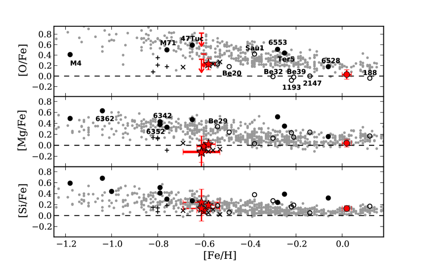
Figure 8.— [X/Fe] ratios of $\alpha$-elements O, Mg, and Si versus metallicity for the stars in our study as well as Galactic field stars and clusters. The red star symbols are the four Pal 1 stars. M67-141 is the red circle. Points with arrows represent upper (or lower) limits. The grey points are Galactic field stars, from the sources assembled by Venn et al. (2004) with additions from Reddy et al. (2006). Black open circles are Galactic OCs from Carraro et al. (2004), Yong et al. (2005), and Friel et al. (2010). Black filled circles are bulge and disk GCs from the sources assembled by Pritzl et al. (2005). Plus signs are stars in Palomar 12 (from Cohen 2004) while crosses are stars in Ter 7 (from Sbordone et al. 2007); both are halo GCs. The dashed lines show solar values.

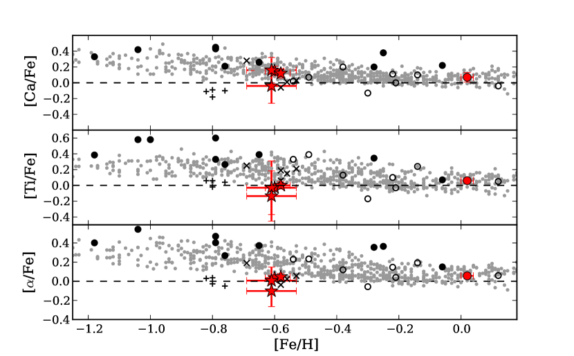
Figure 9.— [X/Fe] ratios of the $\alpha$-elements Ca and Ti, as well as of the average $\alpha$ from Mg, Ca, and Ti. The Ti abundance is an average of Ti I and Ti II, except for Pal 1-I, whose Ti I abundance is shown since its Ti II abundance is abnormally high. The points are as in Figure 8.

The O I lines in our spectral range are the forbidden 6300 and 6363 Å  transitions. Both of these lines are extremely weak and had to measured with spectrum syntheses. Only upper limits are available for Pal 1-I, -II, and -III. Still, the single O abundance seems to follow the general trend of the other $\alpha$-elements. Pal 1-C’s slightly low [O/Fe] value agrees with the lower range of Galactic field star abundances and with the old OCs, particularly Be 20 and 29.

The Mg abundances were determined from lines of varying strengths for M67-141, Pal 1-III, and -C. M67-141 agrees nicely with the field stars. Only one line was detectable in Pal 1-I and -II, and had to be measured with spectrum syntheses. This 5528 Å  line is very strong in all the stars, though it is under the 200 mÅ  limit for the Pal 1 stars. Given that the Pal 1-I and -II abundances agree with -III and -C, they seem reliable. Overall the [Mg/Fe] ratios in Pal 1 are lower than the Galactic field stars, the bulge and disk GCs, and the old OCs, but in agreement with the halo clusters Pal 12 and Ter 7.

The Si abundances were also determined from a wide range of lines, but again only a single line (at 6155 Å) was detectable in Pal 1-I and -II. This line is of intermediate strength in the other two Pal 1 stars, but again the Pal 1-I and -II abundances agree with the others. As discussed in Section 5.5, M67-141’s [Si/Fe] ratio is slightly higher than previous values in the literature; this suggests that Pal 1’s [Si/Fe] might also be slightly high. Its current [Si/Fe] value places it in agreement with the Galactic field stars, the halo GCs, the bulge/disk cluster 47 Tuc, and the old OCs.

The Ca abundance was determined from four to eighteen lines for the Pal 1 stars, with Pal 1-II having the lowest number. All four of these Ca I lines are fairly strong ($>$ 100 mÅ) in Pal 1-II, which has a slightly lower Ca abundance than the other three stars. Again these [Ca/Fe] values agree with Galactic field stars, GCs, and OCs, and the Sgr GCs. M67-141, with 15 Ca lines (most of them strong) matches the [Ca/Fe] values found in the field stars.

A wide assortment of Ti I and II lines were used, of varying strengths. Only three to four Ti I lines were detectable in the Pal 1-I and -II spectra; those lines were of strong and intermediate strength. The other spectra had considerably more Ti I lines. Because many of the Ti II lines are located in the blue regions of our spectra, which have lower SNR, no Ti II lines are detectable in Pal 1-I, and only two intermediate strength lines are detectable in Pal 1-II. Even with only two lines, Pal 1-II’s Ti I and II abundances are in excellent agreement, as are those of Pal 1-III (with 32 Ti II lines), -C (with 23), and M67-141 (with 33). The Ti abundances for M67-141 again follow the field star trend, though Pal 1’s [Ti/Fe] ratios are slightly lower than Galactic field stars, GCs, and OCs. The Pal 12 and Ter 7 [Ti/Fe] ratios are also slightly higher than Pal 1.

Overall, M67-141’s $\alpha$ abundance ratios agree well with the Galactic field stars. Pal 1 shows good agreement with the halo GCs Pal 12 and Ter 7. With the exception of Si and Ca, the [X/Fe] ratios for the $\alpha$-elements in Pal 1 are slightly lower than the bulge and disk clusters and the Galactic field stars. The Galactic [$\alpha$/Fe] ratios are distinct between the thick disk and the thin disk stars; Pal 1 is clearly lower than the thick disk stars, but is not clearly separated from the thin disk. Thus, Pal 1’s [$\alpha$/Fe] ratios are not distinct from the Galactic field stars, GCs, and OCs within the $1\delta$ errors; however, we note that the Pal 1 stars are generally lower than the average Galactic trend.

6.3. Na and Al

Na and Al are also produced in massive stars during nucleosynthesis through carbon burning and hydrogen shell burning (Woosley & Weaver, 1995). The [X/Fe] ratios are shown in Figure 10. Note that Galactic GCs all show star-to-star variations in Na and Al, and the average abundances of the GCs may not reflect the actual primordial abundances. As discussed in Section 5.5, the Na lines with large NLTE corrections have been avoided. Thus, M67-141’s Na abundance is based on the 6154/6161 Å  doublet; the Pal 1 analysis also includes the 5682/5688 Å  doublet. Both Pal 1 and M67-141 have slightly higher [Na/Fe] values than most of the field stars, in agreement with the old OCs and GCs. The Pal 1 [Na/Fe] are distinctly higher than in the halo GCs Pal 12 and Ter 7.

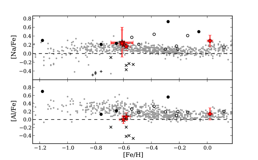
Figure 10.— [X/Fe] ratios of the light elements Na and Al versus metallicity. The points are as in Figure 8.

The Al abundances come from the 6696/6698 Å  lines, both of which are weak in the Pal 1 spectra—thus, [Al/Fe] ratios are not found for Pal 1-I and -II. M67-141’s [Al/Fe] agrees with the field stars, while Pal 1’s [Al/Fe] is slightly low for field stars, bulge/disk GCs, and OCs. As with sodium above, the [Al/Fe] ratios in the Pal 1 stars are distinct from those of stars in Ter 7.

Anticorrelations between Na/O and Al/Mg are seen in nearly all Galactic GCs, and Carretta et al. (2010) suggest that all bona fide GCs show a range in these elements. In Pal 1 Al is clearly not enhanced, and is slightly low for Galactic stars; without significant Al overabundances Mg depletion is not expected to occur (Carretta et al., 2009). Na, however, is slightly enhanced in Pal 1, lying just above the Galactic field stars. In the absence of any stellar evolutionary effects, Na should behave like the $\alpha$-elements, which are also distributed by Type II supernovae. Thus Pal 1’s high Na abundances may indicate that Na-Ne cycled gas is present—since Al is not enhanced, this suggests that Al-Mg cycled gas is not present. With only upper limits on [O/Fe] for three stars, we can only comment that Pal 1-C’s [O/Fe] is slightly low, as expected with higher [Na/Fe]. We further note that there is not a significant range in the [Na/Fe] values for the four stars (see Section 7.1.1) which suggests that the high Na is not a sign of the canonical Na/O anticorrelation seen in Galactic GCs—however, we cannot rule this out with only four stars.

6.4. Iron-Peak Elements

The iron-peak elements are formed in both Type Ia and Type II supernovae, though the precise contributions of the different types are unknown. In Pal 1’s metallicity regime Type Ia supernovae should be the dominant contributors; Iwamoto et al. (1999) estimate that a Type II supernova may create $\sim 0.1\;\rm{M}_{\sun}$ of iron-peak material while a Ia may contribute $\sim 0.8\;\rm{M}_{\sun}$. Figures 11 and 12 show the [X/Fe] ratios of the iron-peak elements. Note that in the single plot for [Cr/Fe] both Cr I (red) and Cr II (yellow) are shown.

6.4.1 Scandium, Vanadium, Manganese, and Cobalt

The odd-Z elements are similar because they have only a single stable isotope each; these elements also require corrections for hyperfine splitting. Note that Sc is included in this discussion, even though it is not a traditional iron-peak element, as its production site is primarily Type II supernovae.

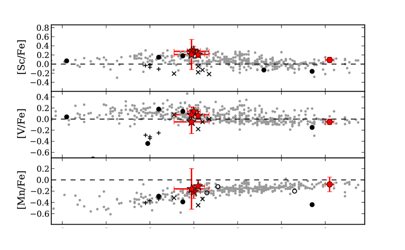
Figure 11.— [X/Fe] ratios of the iron-peak elements Sc, V, and Mn versus metallicity. The points are as in Figure 8.

Sc II and V I have various detectable lines in our spectra. Spectrum syntheses were performed on the 5527 Å  Sc II line for Pal 1-II and on the 6126 Å  V I line for -I. Three intermediate strength Sc II lines (5667, 5669, and 6005 Å) were detectable in Pal 1-I, while four intermediate strength V I lines (6090, 6150, 6199, and 6225 Å) were found in Pal 1-II.

Only four Mn I lines were detectable and under the 200 mÅ  limit in M67-141, all of them strong ($>100$ mÅ). As discussed in Section 5.5, any NLTE corrections to these lines should be small. No Mn I lines were measurable in Pal 1-I, and only a single line (at 6022 Å) was measured in Pal 1-II. The other two Pal 1 stars all have Mn I lines with EWs $<$ 80 mÅ, which should require small NLTE corrections.

Co I has only two lines in this spectral range, at 5483 and 5647 Å. Neither line was detected in Pal 1-I or -II. In M67-141, Pal 1-III, and -C the 5483 Å  line is intermediate or strong while the 5647 Å  line is weak to intermediate.

All of Pal 1’s odd iron-peak elements agree with the Galactic field stars. Sc is slightly higher than the general Galactic trend, putting Pal 1 in closer agreement with 47 Tuc than with Ter 7 or Pal 12. The V abundances are slightly lower than the Galactic trend, in agreement with field stars and Ter 7. [Mn/Fe] is slightly higher than all the GCs, but agrees with field stars and the old OCs Be 20 and 29. Finally, [Co/Fe] is slightly low, in agreement with the halo clusters but still within range for OCs and field stars—a comparison cannot be made with the GCs as Co abundances are not available for all clusters.

6.4.2 Chromium and Nickel

There are 11 available Cr I lines in our line list, but only two Cr II lines, both of which are in the blue spectral regions. Thus, Cr II abundances are not available for Pal 1-I and -II; unfortunately, the redder Cr I lines were also not measurable in Pal 1-I and -II. For the other stars the Cr I abundances are in good agreement with each other and with the literature. M67-141 looks like Galactic field stars and GCs, while Pal 1 lies slightly below the field stars and agrees with the halo GCs. However, the Cr II abundances are considerably higher (identified as yellow in Figure 12), an effect that has been observed in previous studies of Galactic stars (e.g. Zhang et al. 2009). The Cr II abundances may not be reliable because the lines are in the blue regions of our spectra; however, the discrepancy between Cr I and Cr II may be due to NLTE effects for Cr I (Sobeck et al., 2007; Bergemann & Cescutti, 2010). Therefore, neither [Cr I/Fe] nor [Cr II/Fe] may be valuable choices for comparisons.

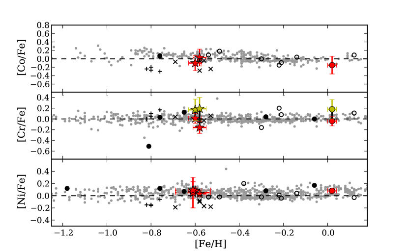
Figure 12.— [X/Fe] ratios of the iron-peak elements Co, Cr, and Ni versus metallicity. Both Cr I and Cr II are shown (Cr I in red, Cr II in yellow); note that the low SNR stars Pal 1-I and -II only have Cr I abundances. The points are as in Figure 8.

Ni also has many spectral lines, though only three and five are detectable in Pal 1-I and -II, respectively. Both M67-141 and Pal 1’s [Ni/Fe] values match those of field stars and clusters, with the exceptions of Ter 7 and Pal 12, which are slightly lower.

6.5. Copper and Zinc

The nucleosynthetic origins of Cu and Zn are varied, and the precise yields from various sites depend on the models used. Explosive burning in Type Ia and II supernovae can create Cu and Zn, as can neutron captures. Given the uncertainty surrounding the formation of these elements they are discussed separately from the rest. Their [X/Fe] ratios are shown in Figure 13.

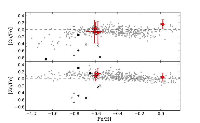
Figure 13.— [X/Fe] ratios of the elements Cu and Zn versus metallicity. The points are as in Figure 8.

Three Cu I lines are examined here: 5105.5, 5700, and 5782 Å. These lines are all strong in M67-141, though the last two are $<100$ Å  in the Pal 1 stars. None are detectable in Pal 1-I, while only the last is detectable in Pal 1-II. The 5782 Å  line was just off the end of the red region in Pal 1-III and Pal 1-C, and the 5700 Å  line was obscured by a cosmic ray in Pal 1-C. The three Pal 1 [Cu/Fe] ratios agree with the field stars. However, the [Cu/Fe] values are not within $1\delta$ of Ter 7 and Pal 12. M67-141’s [Cu/Fe] is a bit high, but its $1\delta$ errors place it with the Galactic field stars.

Three intermediate strength Zn I lines lie in our spectral region, at 4722, 4811, and 6362 Å, and yield consistent abundances when all three are measured in one star. None are detectable in Pal 1-I or -II, though all three are measurable in M67-141, Pal 1-III, and Pal 1-C. Similar to copper, both M67-141 and Pal 1 have [Zn/Fe] ratios that agree with field stars and GCs but are higher than Ter 7 and Pal 12.

6.6. r- and s-Process Elements

The heavier elements are formed through neutron captures onto iron-peak atoms, either via the rapid (r-) process in Type II supernovae, or via the slow (s-) process, e.g. in low mass AGB stars. In the Sun, the percentages of Y, Ba, La, Nd, and Eu that come from the s-process are 75%, 85%, 72%, 47%, and 3%, respectively (Burris et al., 2000); thus Eu is an important r-process indicator. The [X/Fe] ratios for the elements that are primarily due to the s-process (Y, Ba, and La) are shown in Figure 14, while those with larger r-process contributions (Nd and Eu) are shown in Figure 15.

6.6.1 s-Process Elements

Five Y II lines are detectable in the Pal 1 spectra, all in the blue: 4884, 4900, 5087, 5200, and 5403 Å. The first four lines are of intermediate-strength in the Pal 1 stars while the last is weak. All five lines yield consistent abundances when measured in one star. Spectrum syntheses were performed on the 5087 and 5200 Å  lines for Pal 1-I and on the 5200 and 5403 Å  lines for -II; only upper limits are given. While M67-141 agrees well with the field stars, the Pal 1 stars are deficient in [Y/Fe] compared to field stars and globular clusters. The Pal 1 [Y/Fe] ratios are in better agreement with those from Ter 7 and Pal 12.

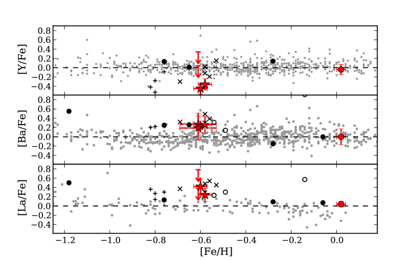
Figure 14.— [X/Fe] ratios of the elements Y, Ba, and La versus metallicity. The points are as in Figure 8, with additional Galactic abundances from Simmerer et al. (2004).

Ba II and La II have three and four lines, respectively, in our line list. As mentioned in Section 5.2, spectrum syntheses were performed on all the 6142 Å  lines to include the effect of the blended Ni I line. Another Ba II line, 4934 Å, was quite strong and was not always below the 200 mÅ  limit. The remaining Ba II line, 5853 Å, is of intermediate to strong strength. The four La II lines (5302, 5304, 6320, and 6774 Å) are all weak in the Pal 1 stars. Spectrum syntheses were performed on the 6774 Å  line to obtain upper limits for Pal 1-I and -II. [Ba/Fe] and [La/Fe] show a similar trend in Figure 14: both are higher in Pal 1 than in the field stars, but both are in agreement with 47 Tuc, Ter 7, Pal 12, and the old OCs, particularly Be 29.

High s-process yields have been observed in Galactic GC (e.g. M4, Yong et al. 2008), and have typically been explained by primordial variations, i.e. the cluster happened to be born in a region where all s-process yields were particularly high. However, in Pal 1 not all the s-process elements are high: Y, a first-peak s-process element, shows the opposite trend from Ba and La, which are second-peak elements. To compare the relative contributions of second-peak to first-peak, [Ba/Y] vs. [Fe/H] is shown in the top panel of Fig. 16. Though only lower limits are available for Pal 1-I and -II, it is still evident that Pal 1 has higher [Ba/Y] ratios than the field stars and GCs, though it is in good agreement with the ratios for Ter 7 and Pal 12.

6.6.2 r-Process Elements

Five Nd II lines are observable in M67-141. Of these five, only two (5250 and 5320 Å) are strong enough to be seen in the Pal 1 stars. Only the latter line was detected in Pal 1-I; no Nd II lines were found in Pal 1-II. The 6645 Å  Eu II line required spectrum syntheses for all stars; again, only upper limits were obtained for Pal 1-I and -II.

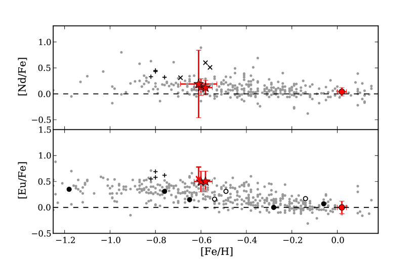
Figure 15.— [X/Fe] ratios of the elements Nd and Eu versus metallicity. The points are as in Figure 14.

Figure 15 shows that M67-141 follows the field star trend for both Nd and Eu, while Pal 1, though slightly high, is still in agreement with the Galactic field stars within its $1\delta$ errors. Pal 1’s [Nd/Fe] ratio may be a bit low compared to Ter 7 —no comparisons are available for the other Galactic GCs. The [Eu/Fe] of the Pal 1 stars is in good agreement with Pal 12, but those are both much higher than in 47 Tuc and other Galactic GCs and OCs.

Since 97% of Eu is produced via the r-process in the Sun (Burris et al., 2000), it is primarily an r-process indicator. Also, since the site of the r-process is believed to be Type II supernovae, which also distribute the $\alpha$-elements, then the $[\rm{Eu}/\alpha]$ ratio should be correlated. The middle panel in Figure 16 shows $[\rm{Eu}/\alpha]$ vs. [Fe/H]. Pal 1 has higher $[\rm{Eu}/\alpha]$ ratios than the Galactic field stars, GCs, and OCs, but is in good agreement with the $[\rm{Eu}/\alpha]$ ratios in Ter 7 and Pal 12. The excess Eu relative to the Galactic stars suggests different yields for Eu and $\alpha$ elements, and that whatever the source of these different yields, it was similar for Pal 1, Ter 7, and Pal 12.

6.6.3 s-Process vs. r-Process

The ratio [Ba/Eu] provides a clue of the ratio of the s- to r-process contributions. The bottom panel in Figure 16 shows that Pal 1 is in good agreement with the Galactic field star distribution, suggesting that in Pal 1 the s-process contributes to the chemical evolution in a similar way as in the Galaxy. It is interesting that Pal 1’s [Ba/Eu] ratios are similar to Pal 12 and Be 20, but that those are all slightly lower than the rest of the Galactic GCs and OCs.

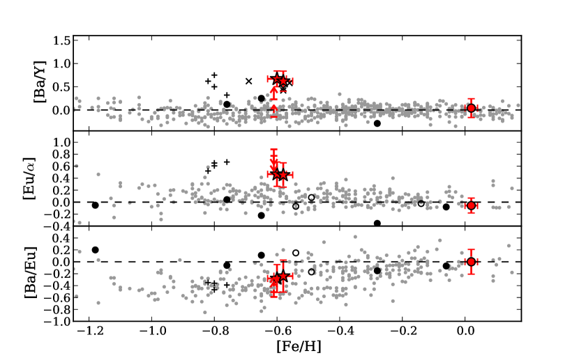
Figure 16.— [Ba/Y], [Ba/Eu], and [Eu/$\alpha$] versus metallicity. The points are as in Figure 14.

7. Discussion

With the derived abundances of twenty one different elements, the guiding questions of this analysis can be addressed. Ultimately we wish to understand what type of cluster Pal 1 is and whether or not it has been accreted from a satellite galaxy. The answers to these questions may have implications for galaxy and cluster formation.

7.1. What Kind of a Cluster is Pal 1?

As discussed in Section 1, Pal 1 has traditionally been classified as a GC, primarily because of its location above the Galactic plane and its high concentration parameter. However, Pal 1’s high [Fe/H] and red horizontal branch make it similar to the bulge/disk GCs (Mackey & Van Den Bergh, 2005), while its age sets it apart from all GCs. In fact, its age and [Fe/H] place it between the classical definitions of GCs and OCs. These unusual characteristics have caused Pal 1 to be labeled as a “transitional cluster” (Ortolani et al., 1995).

In addition, Pal 1’s brightness and size make it an ultra faint cluster. A graph of absolute magnitude versus half-light radius (see Figure 1 in Niederste-Ostholt et al. 2010) shows that Pal 1 is fainter than typical globular clusters and occupies a position that could be an extrapolation of the dwarf galaxy and ultra faint dwarf galaxy trend. It is therefore worth investigating Pal 1’s similarities to these different types of objects.

7.1.1 Basic Properties of Pal 1

We begin by summarizing the basic properties of Pal 1 that have been determined in this paper. We have derived a average metallicity of $[\rm{Fe/H}]=-0.60\pm 0.01$ for Pal 1, a result that is in agreement with both the CaT estimates (Rosenberg et al., 1998b) and the isochrone fits (Sarajedini et al., 2007). We further find that the cluster is not $\alpha$-enhanced. Defining $\alpha$ to be an average of Mg, Ca, and Ti, the average $[\alpha/\rm{Fe}]\approx 0.0$.

A revised age can be derived using our updated, detailed abundances. Isochrones from the Dartmouth Stellar Evolution Database (Dotter et al., 2008) have been adopted to derive a new age for Pal 1 using the derived $[\rm{Fe/H}]\approx-0.6$ and $[\alpha/\rm{Fe}]\approx 0.0$ (previously values of $[\rm{Fe/H}]=-0.7$ and $[\alpha/\rm{Fe}]=0.2$ were used, Sarajedini et al. 2007). The same distance modulus and reddening are used as for the photometric atmospheric parameters: $(m-M)_{0}=15.65$ and $E(B-V)=0.20$ (see Section 4.2 for details); the photometry is taken from the Sarajedini et al. (2007) HST Globular Cluster Treasury.

Fits of the Dotter et al. (2008) isochrones are shown in Figure 1, for ages of 4, 5, and 6 Gyr; the best age remains at $5\pm 1$ Gyr. The differences between these fits and those of Sarajedini et al. (2007) are very slight, as expected since the adopted [Fe/H] and [$\alpha$/Fe] combinations correspond to roughly the same [M/H]. Thus, our analysis confirms the previous findings that Pal 1 is indeed a young cluster. We further note that none of our target red giant stars lie on the isochrone RGBs; this may suggest that our targets are actually horizontal branch stars.

No conclusive signs of any abundance spreads are detected among the four Pal 1 stars, suggesting that Pal 1 is indeed a simple stellar population. Table 10 shows the mean [X/Fe] ratios in Pal 1 and the abundance spreads within the cluster, according to the method outlined in Cohen (2004). Here $\sigma$ is the dispersion about the mean abundance in the cluster and $\sigma$(obs) is the mean uncertainty of an element in a single star. The spread ratio is then a comparison of the width of the mean distribution to the width of a single star’s error estimate: large values of the spread ratio imply that the star-to-star variations are larger than the average uncertainty for an individual star, suggesting that the cluster has a genuine abundance spread. The Pal 1 stars do not show a significant spread for most elements (a spread ratio $>1.0$ would be considered significant; Cohen 2004). Cr I has a spread ratio $>1.0$, but abundances are only available for 2 stars. The low spread ratio for Na suggests that a Na/O anticorrelation is not present, although O is available for only one star. Thus, Pal 1 does not appear to show any signs of star-to-star variations. This is further confirmed by its CMD: multiple populations are not evident and a single isochrone fits it well, implying that the cluster is coeval.

Table 10Mean abundances and spread ratios for the four stars in Pal 1, according to the method of Cohen (2004). A spread ratio $>1$ indicates that a significant spread exists; Pal 1 shows no evidence for any abundance spreads. See the text for a description of how these values are calculated.

	Mean [X/Fe]	Number of stars	$\sigma$	$\sigma$(obs)	Spread Ratio
Fe I	-0.60	4	0.01	0.06	0.26
Fe II	-0.60	4	0.10	0.21	0.46
Na	0.21	4	0.04	0.21	0.21
Mg	-0.06	4	0.07	0.16	0.44
Al	0.04	2	0.05	0.10	0.49
Si	0.16	4	0.07	0.15	0.45
Ca	0.10	4	0.09	0.13	0.75
Sc	0.25	4	0.05	0.19	0.25
Ti I	-0.06	4	0.07	0.21	0.33
Ti II	-0.04	3	0.11	0.21	0.52
V	0.06	4	0.08	0.12	0.68
Cr I	-0.09	2	0.12	0.10	1.20
Cr II	0.18	2	0.01	0.21	0.07
Mn	-0.16	3	0.05	0.18	0.27
Co	-0.04	2	0.09	0.20	0.47
Ni	0.06	4	0.03	0.12	0.22
Cu	-0.03	3	0.06	0.28	0.23
Zn	0.12	2	0.05	0.15	0.34
Y	-0.41	2	0.06	0.12	0.53
Ba	0.24	4	0.04	0.20	0.18
La	0.33	2	0.13	0.15	0.85
Nd	0.15	3	0.04	0.32	0.12
Eu	0.50	2	0.0	0.20	0.0

Thus, our analysis finds Pal 1 to be a metal-rich, non-$\alpha$-enhanced, young, chemically homogeneous stellar population.

7.1.2 Globular or Open Cluster?

Given that the cluster types are not well-defined it is difficult to distinguish between the two types of clusters, particularly when examining chemical abundances. However, multiple populations have been observed in nearly all Galactic GCs, but not in open clusters. Thus, signs of the Na/O and/or the Mg/Al anticorrelations would be positive indicators for a GC.

No signs of the Mg/Al anticorrelation are detected in Pal 1, and O abundances are only available for one of the four stars, Pal 1-C. As discussed in Section 6.3, while Na is slightly high and O is slightly low in Pal 1-C, there is no significant range in the Na abundances, and the four stars do not show evidence for an anticorrelation. Certain models (e.g. Conroy & Spergel 2011) suggest that the formation of a second population in a GC depends on the cluster mass, since more massive clusters can retain more gas to form a second population—Pal 1’s current mass, $\log(M/\rm{M}_{\sun})\approx 3.2$ (Niederste-Ostholt et al., 2010), is below the critical mass for retaining the gas to form a second population. It has been known for some time that Pal 1 is in the process of evaporating (Rosenberg et al., 1998a); Niederste-Ostholt et al. (2010) further show that the mass in Pal 1’s tidal tails is roughly equal to its current mass, suggesting that the cluster might have been at least twice as massive in the past. In the Conroy & Spergel (2011) context, however, Pal 1’s lack of a second generation implies that it was never more massive than $\log(M/\rm{M}_{\sun})=4.0$, regardless of its current size. This restriction is not necessarily unusual for a GC: the GC Pal 12 does not show signs of abundance spreads (Cohen, 2004) and five intermediate age ($<2$ Gyr) LMC GCs show no evidence for multiple populations in their CMDs.

Pal 1’s detailed abundances can also be compared to the well-established GCs in the Galaxy. Its metallicity alone puts it in an unusual regime: while there are many metal-rich GCs, those are usually centrally concentrated in the bulge or disk, while Pal 1 is located much further from the center and far above the disk ($R_{\rm{GC}}=17.2$ kpc and $Z=3.6$ kpc; Harris 1996, 2010 edition). Most of the iron-group (Figures 11 and 12), $\alpha$- (Figures 8 and 9), and neutron capture elements (Figures 14, 15, and 16) are in good agreement between Pal 1 and the Sgr clusters; however, the Na, Al, Cu, and Zn abundances (Figures 10 and 13) are distinctly different. Thus, the chemical pattern of Pal 1 is not clearly similar to either the metal-rich Galactic GCs or the Sgr GCs. Of the GCs, Pal 1 is most similar to Pal 12 and Ter 7, both known to be associated with the Sgr dSph.

There are several old, metal-poor OCs with detailed abundances in the literature, though most are more metal-rich than Pal 1. Several of these clusters are located in the outer disk, and may have been accreted from a dwarf galaxy or formed during a major merging event (Yong et al., 2005). Be 20 and 29, the two clusters in our sample that lie closest to Pal 1’s metallicity, have similar abundance ratios as the Galactic stars, with the exceptions of the s-process neutron capture elements. Thus, the only elements that are clearly discrepant between Be 20/29 and Pal 1 are the $\alpha$-elements (Figures 8 and 9) and Eu (and by extension [Eu/$\alpha$] and [Ba/Eu]; Figures 15 and 16). Cu, Zn, and Y abundances are not available for Be 20 and 29; however, Pal 1’s Na and Al abundances (Figure 10) agree better with Be 20 and 29 than with the Sgr clusters.

It is then natural to ask if Pal 1 looks more like the GCs Pal 12 and Ter 7 or the OCs Be 20 and 29. In terms of the $\alpha$-elements and neutron capture elements Pal 1 looks more like the GCs, while Na and Al agree more with the OCs. However, chemically comparing Pal 1 to the two cluster types is not an accurate way of determining Pal 1’s cluster type, as Pal 1, Be 20, and Be 29 are not conclusively associated with dwarf galaxies while Pal 12 and Ter 7 are associated with the Sgr dSph. Furthermore, the chemical abundances of stars depend on their host galaxies’ star formation histories, etc., and these quantities are unique to individual galaxies. Thus, unless all of the clusters originated in the Sgr dSph, this comparison is not straightforward. We leave the question of Pal 1’s origin to Section 7.2 and we therefore focus on other parameters that may distinguish GCs from OCs.

Table 11 shows various quantities that can be compared between the clusters: the Galactocentric radius, $R_{\rm{GC}}$ (in kpc); the distance above the Galactic plane, $Z$ (in kpc); distance from the Sun, $d$ (in kpc); the age (in Gyr; though note that these ages are assembled from different sources, and may not be valid for comparisons); metallicity, [Fe/H]; absolute visual magnitude, $M_{V}$; half-light radii, $r_{h}$ (in pc; note that the distance was used to convert the half-light radius from arcminutes to pc); and concentration parameter, $c$. The last two parameters are only available for the GCs. Note that we also include Whiting 1, a GC associated with Sgr (Carraro et al., 2007), though there are no chemical abundances available for this cluster at this time. The values of $R_{\rm{GC}}$ are similar for all the clusters in the table. The OCs, while more than 1 kpc away from the plane, are still closer than the GCs, with Pal 1 lying between the two. The ages and metallicities are similar, but again Pal 1 is still quite young for a GC. Though Pal 1 is fainter than the OC Be 29, its brightness is comparable to the GC Whiting 1. Finally, Pal 1 has a very small half-light radius compared to Pal 12 and Ter 7, but in agreement with Whiting 1, and Pal 1 is very concentrated, much more so than Ter 7 and Whiting 1.

Table 11Various parameters for the GCs and OCs used in this study. If no references are given then the data comes from this study (in the case of Pal 1) or the Harris (1996) catalog (2010 edition). Note that the ages are assembled from different sources, and therefore might not be directly comparable. All values of $|Z_{\rm{Sgr}}|$ are from Law & Majewski (2010).

Cluster	Traditional	$R_{GC}$	$Z$	$d$	age	[Fe/H]	$M_{V}$	$r_{h}$	$c$	$|Z_{\rm{Sgr}}|$	References
	Classification	(kpc)	(kpc)	(kpc)	(Gyr)			(pc)		(kpc)
Pal 1	?	17.2	3.6	14.2	5.0	-0.6	-2.52	1.8	2.57	9.8
Pal 12	GC	15.8	-14.1	19.0	9.5	-0.80	-4.47	9.1	2.99	3.24	1, 2
Ter 7	GC	15.6	-7.8	22.8	8.0	-0.60	-5.01	4.9	0.93	1.09	1, 3
Whiting 1	GC	34.5	-26.3	30.1	6.5	-0.65	-2.46	1.8	0.55	0.215	4
Be 20	OC	15.8	-2.5	-	5.8	-0.44	-2.06	-	-	-	5, 6, 7
Be 29	OC	21.6	1.8	-	4.5	-0.54	-4.64	-	-	1.79	4, 6, 8
Saurer 1	OC	19.2	1.7	-	5.0	-0.38	-	-	-	5.25	4, 9

The distinctions between OC and GC in Table 11 seem to be based primarily on distance from the Galactic plane. Considering that Pal 12, Ter 7, and Whiting 1 have been accreted by Sgr, this is not a particularly valid criterion. Consequently, the distance above the Sgr plane, $|Z_{\rm{Sgr}}|$, is also plotted for clusters that are (or might be) associated with the Sgr dSph (from Law & Majewski 2010; note that Pal 1’s $|Z_{\rm{Sgr}}|$ is also included, although it is most likely not associated with Sgr). Examined this way, the clusters look very similar, i.e. the young, metal-rich GCs that are close to the Sgr plane are similar to the old, metal-poor OCs that are close to the Galactic plane, suggesting that these clusters may be classified as open (or intermediate-aged) clusters in the Sgr frame of reference. Carretta et al. (2010) also cast doubt upon the GC classification for Pal 12 and Ter 7, given the lack of a definite Na/O anticorrelation. Under the Carretta et al. definition we are forced to conclude that Pal 1 is not a bona fide GC; however, it is not an obvious Galactic OC either, and therefore remains as an unusual cluster.

7.1.3 A Connection with Ultra-Faint Dwarfs?

Given Pal 1’s identification as an ultra faint cluster and its proximity to the ultra-faint dwarfs (UFDs) in a plot of absolute magnitude vs. half-light radius (Figure 1 in Niederste-Ostholt et al. 2010) it is tempting to consider whether Pal 1 is related to these other ultra-faint objects. The UFDs are distinguished by their larger-than-expected velocity dispersions, which imply high mass/light ratios and large amounts of dark matter. The velocities for the five Pal 1 stars (including Pal 1-IV) listed in Table 2 imply a velocity dispersion of $3.6\pm 1.5$ km s^-1 (using the formula from Walker et al. 2006), assuming that all five velocities are orbital velocities of cluster members. Under this assumption, Pal 1’s velocity dispersion is in agreement with the velocity dispersions of several UFDs, including Segue II, Leo V, Leo IV, and Hercules (see the summary of UFD properties by McConnachie & Côté 2010).

As tempting as this comparison may be, it is not altogether appropriate. Firstly, we now know that Pal 1 has tidal tails and is therefore not in dynamical equilibrium (Niederste-Ostholt et al., 2010). Secondly, only one star (Pal 1-IV) has a discrepant velocity, and this difference is easily explained if Pal 1-IV is a binary; McConnachie & Côté (2010) showed that the presence of binaries can significantly boost the velocity dispersion of a low-mass system. Alternatively, Pal 1-IV could be a nonmember—its location in the CMD (Figure 1) is separate from the other stars—however its consistent chemistry and very close radial velocity make this seem unlikely. Therefore, Pal 1 remains an ultra faint cluster, and though it would be interesting if it were an extrapolation of the UFDs, its current velocity dispersion is best explained by its tidal disruption or by the presence of a binary.

7.2. Is Pal 1 Extragalactic?

Pal 1 has been tentatively associated with both the Galactic Anticenter Stellar Stream (GASS) (Crane et al., 2003) and the Canis Major (CMa) overdensity (e.g. Martin et al. 2004, Forbes & Bridges 2010), two streams of stars that could be from disrupted dwarf galaxies. If it is associated with either of these systems, then Pal 1 should have similar chemical abundances to their associated field stars and clusters and to the stars in other low mass systems.

Figures 17 through 25 compare the Pal 1 abundances to those of stars in the nearby dwarf galaxies. Note that only the average Pal 1 abundance (red star symbol) is plotted, with the mean abundance error for [X/Fe] (e.g. $\sigma$(obs) in Table 10). The Galactic field stars are shown in grey. Dwarf galaxies are also included, with their field stars as small symbols and their GCs as larger open symbols. Again, abundances have been averaged over an entire cluster. Black points are Fornax stars (Letarte et al., 2010); cyan triangles are Sagittarius (Sgr) stars (field stars are from Sbordone et al. 2007, Monaco et al. 2007, and Chou et al. 2010a, while GC stars are from Cohen 2004 and Sbordone et al. 2005b); blue squares are Large Magellanic Cloud stars (field stars from Pompéia et al. 2008; cluster stars from Johnson et al. 2006 and Mucciarelli et al. 2008); green crosses are Galactic Anticenter Stellar Stream (GASS; Chou et al. 2010b) stars; and orange diamonds are field stars in the Canis Major overdensity (Sbordone et al., 2005a). While other dwarf galaxy data are available in this metallicity range, plotting all of it makes these plots nearly illegible, and we have therefore included only the most relevant dwarf data (i.e. galaxies with many stars and many elemental abundances in the same metallicity range as Pal 1) for this discussion.

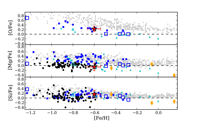
Figure 17.— [X/Fe] ratios of $\alpha$-elements O, Mg, and Si versus metallicity for the stars in our study as well as Galactic field stars (grey; as in Figure 8) and stars in other galaxies. Black points are Fornax stars (Letarte et al., 2010); cyan triangles are Sagittarius (Sgr) stars (field stars are from Sbordone et al. 2007, Monaco et al. 2007, and Chou et al. 2010a, while GC stars are from Cohen 2004 and Sbordone et al. 2005b); blue squares are Large Magellanic Cloud stars (field stars from Pompéia et al. 2008; cluster stars from Johnson et al. 2006 and Mucciarelli et al. 2008); and orange diamonds are field stars in the Canis Major overdensity (Sbordone et al., 2005a).

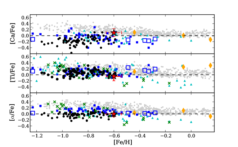
Figure 18.— [X/Fe] ratios of the $\alpha$-elements Ca and Ti, as well as of the average $\alpha$ from Mg, Ca, and Ti. The Ti abundance is an average of Ti I and Ti II, except for Pal 1-I, whose Ti I abundance is shown since its Ti II abundance is abnormally high. The points are as in Figure 17, with the addition of Galactic Anticenter Stellar Stream (GASS; green crosses) stars from Chou et al. (2010b).

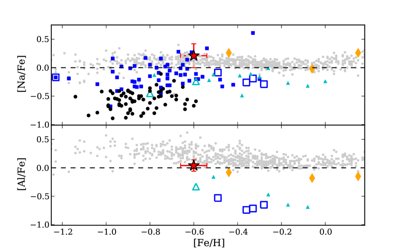
Figure 19.— [X/Fe] ratios of the light elements Na and Al versus metallicity. The points are as in Figure 17.

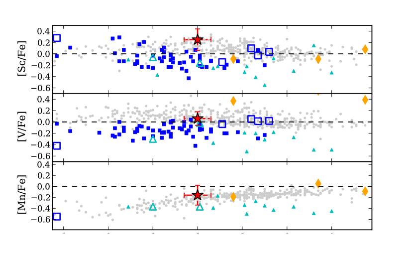
Figure 20.— [X/Fe] ratios of the iron-peak elements Sc, V, and Mn versus metallicity. The points are as in Figure 17.

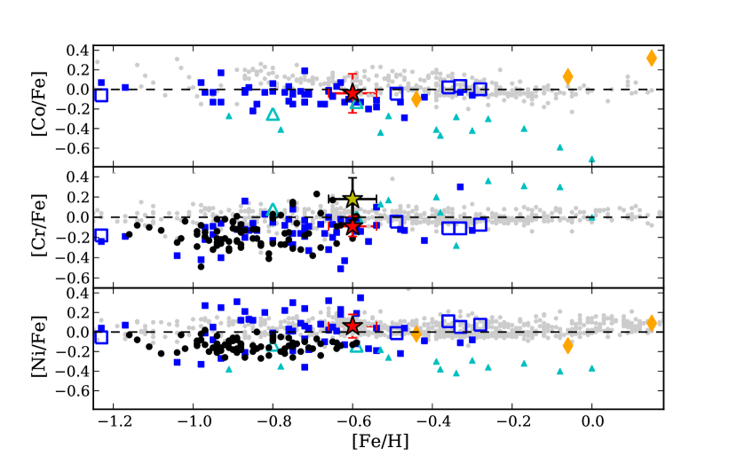
Figure 21.— [X/Fe] ratios of the iron-peak elements Co, Cr, and Ni versus metallicity. Both Cr I and Cr II are shown (Cr I in red, Cr II in yellow). The points are as in Figure 17.

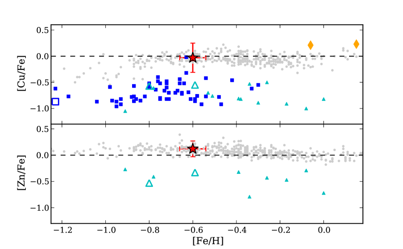
Figure 22.— [X/Fe] ratios of the elements Cu and Zn versus metallicity. The points are as in Figure 17.

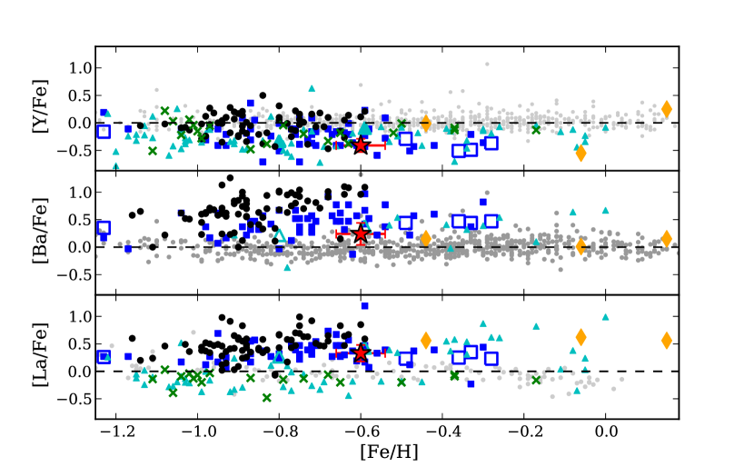
Figure 23.— [X/Fe] ratios of the elements Y, Ba, and La versus metallicity. The points are as in Figure 18.

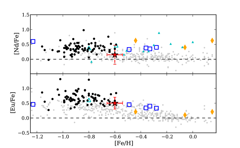
Figure 24.— [X/Fe] ratios of the elements Nd and Eu versus metallicity. The points are as in Figure 17.

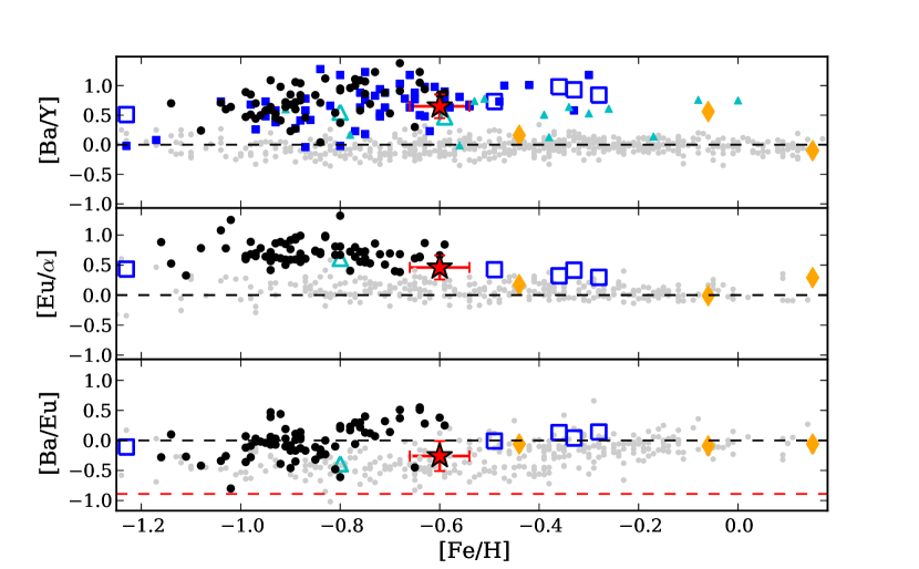
Figure 25.— [Ba/Y], [Ba/Eu], and [Eu/$\alpha$] versus metallicity. The dashed red line shows the r-process-only [Ba/Eu] ratio (from Burris et al. 2000). The points are as in Figure 17.

7.2.1 General Comparisons: Dwarf Galaxy or MW cluster?

In terms of the $\alpha$-elements (Figures 17 and 18), Pal 1’s slightly low [$\alpha$/Fe] ratios place it with the dwarf galaxies (with the possible exception of Ca). This suggests that Type Ia supernovae began to contribute to Pal 1’s host environment at a lower [Fe/H] than for stars in the Galaxy. In general, Pal 1’s [$\alpha$/Fe] ratios agree with the Sgr and LMC clusters. The slightly subsolar [Ti/Fe] value agrees with the GASS stars while the slightly low [Mg/Fe] and [Ti/Fe] and slightly higher [Ca/Fe] and [Si/Fe] ratios agree with the $[\rm{Fe/H}]=-0.44$ CMa star. The latter CMa star is also similar to Pal 1 in Na and Al (Figure 19); for the few available [Al/Fe] abundances Pal 1 is higher than the Sgr and LMC clusters.

Of the iron-peak elements (Figures 20 and 21), Pal 1’s [Sc/Fe] remains clearly distinct from the dwarf galaxy stars. Pal 1’s [V/Fe] ratio is in good agreement with the dwarfs, with the exception of the CMa stars, which may be due to HFS corrections. Overall the Pal 1 Fe-peak elements show the best agreement with the Galactic stars rather than the dwarf galaxy stars. Variations in [Fe-peak/Fe] with metallicity have been suggested to be due to metallicity-dependent supernovae yields, e.g. metal-poor Type Ia supernovae will produce less Mn than metal-rich ones (Cescutti et al., 2008), as seen in the Sgr field stars. However, Pal 1’s agreement with the Galactic and dwarf galaxy stars at a similar metallicity suggests no significant dispersion in the Type Ia contributions. The more peculiar elements, Cu and Zn (Figure 22), are in better agreement with the Galactic stars and possibly CMa, and are clearly distinct from the Sgr and LMC stars.

Finally, Pal 1’s neutron capture elements (Figures 23, 24, and 25) agree better with the dwarf galaxies than with the Galactic stars. Pal 1’s low [Y/Fe] and high [Ba/Fe], [La/Fe], and [Ba/Y] ratios suggest that like the Sgr dSph, Pal 1 was enriched by metal-poor AGB stars. (This effect is also seen in the [La/Y] ratios of the Sgr stars; McWilliam & Smecker-Hane 2005). With an excess of neutrons per Fe atom in metal-poor AGB stars, more heavy second-peak s-process elements such as Ba and La can be created, leaving a deficit of first-peak elements like Y (Gallino et al., 1998; Bisterzo et al., 2010). This further suggests that Pal 1 has not been enriched by its own metal-rich AGB stars, which is perhaps not surprising given its lack of evolved stars (see Figure 1). The GASS field stars do not have high [La/Fe] like Pal 1, suggesting that it does not have an excess of second-peak to first-peak s-process elements. The CMa stars do seem to have high [Ba/Fe] and [La/Fe], and arguably have low [Y/Fe], in agreement with Pal 1.

Pal 1 also has slightly higher [Eu/Fe], [Nd/Fe], and [Eu/$\alpha$] ratios than Galactic stars, in agreement with the LMC, Sgr, and Fornax. While the CMa stars do show an excess of Nd, they do not appear to have an excess of Eu, and CMa therefore has a normal value for [Eu/$\alpha$]. This suggests that dwarf galaxies have an additional source of r-process elements compared to the Galaxy (see e.g. Letarte et al. 2010). This is further supported by Pal 1 and the dwarf galaxies’ high [Eu/$\alpha$] ratio; the standard model suggests that massive Type II supernovae are responsible for dispersing the $\alpha$-elements, while lower mass (8-10 M_☉) Type II supernovae are the sole site of r-process elements like Eu. If the dwarf galaxies had similar conditions to the Galaxy, then the [Eu/$\alpha$] ratio should remain flat.

Despite its high values for [Ba/Fe] and [Eu/Fe], the [Ba/Eu] ratio in Pal 1 agrees better with the Galactic stars than with the dwarf galaxies, though the Fornax dispersion and Pal 12 do extend down to Pal 1’s value. Again CMa’s [Ba/Eu] values are in fair agreement with Pal 1.

As discussed earlier, at solar metallicity Ba is primarily an s-process element, while Eu is primarily an r-process element (Burris et al., 2000). The ratio [Ba/Eu] should therefore provide an indication of the relative contributions of the s-process to the r-process. Before the s-process begins to contribute Ba is initially produced solely through the r-process; as time goes on the s-process creates more Ba but little Eu, and [Ba/Eu] increases. The theoretical r-process–only lower limit for [Ba/Eu] is shown in Figure 25. Pal 1’s slightly high Ba and Eu abundances lead to a [Ba/Eu] value that agrees with the classical prediction for a system that has had little contribution from the s-process. Clearly this cannot be the case: Pal 1’s [$\alpha$/Fe] ratios show that Type Ia supernovae have contributed to the system, and therefore AGB stars must have also contributed since the timescale for evolution of Type Ia supernovae and AGB stars is thought to be similar in chemical evolution models (e.g. Travaglio et al. 2004, Matteucci et al. 2009, Zolotov et al. 2010). The [Ba/Y] ratio further implies that metal-poor AGB stars must have contributed to the system. Thus, the high [Eu/Fe] and [Ba/Fe] together with the high [Eu/$\alpha$] suggest that there is an extra source of r-process elements in the Pal 1 system, beyond what is present for typical Galactic stars. It is unclear where the additional r-process abundances come from; some possibilities include shot noise (i.e. simple inhomogeneous mixing of a nearby supernova with a progenitor in the 8-10 M_☉ range), an unusual star formation history that may have included an effectively truncated IMF (missing the most massive stars that contribute significantly to the $\alpha$ elements), or even variable nucleosynthetic yields. However, each of these possibilities has other consequences for the chemical abundance ratios that are not clearly indicated in Pal 1. Whatever the case, Pal 1 has clearly not followed the “classical” chemical evolution models.

Based on these chemical comparisons, we conclude that Pal 1 likely originated in a dwarf satellite that was later accreted by the Milky Way (about 500 Myr ago; Niederste-Ostholt et al. 2010). Though the light elements ($Z\leq 30$) are arguably in agreement with Galactic disk stars, the neutron capture elements are distinct enough for us to conclude that Pal 1 does have an extragalactic origin.

7.2.2 Comparisons with Specific Galaxies: Pal 1’s Host Galaxy?

We now attempt to chemically link Pal 1 to its host galaxy, as has been done with e.g. Pal 12 (Cohen, 2004) and Ter 7 (Sbordone et al., 2005b). In particular we examine the chemical abundances of the CMa overdensity, the GASS, and the LMC intermediate-age clusters.

Given the low [La/Fe] abundance in the GASS, it is not likely that Pal 1 is a member of this stream. The few stars analyzed in the CMa overdensity are more promising (even if the stars analyzed so far in CMa are more metal-rich): the general trends in the $\alpha$-abundances, the odd-Z elements Na, Al, Cu, and Zn, the iron-peak elements (with the exception of Sc and V possibly due to HFS corrections), and the neutron capture elements (possibly with the exception of Eu) are in fair agreement. Based on this analysis it is possible that Pal 1 could be associated with this stream, as suggested by Saviane et al. (2010) and Forbes & Bridges (2010). The slight differences between individual elements could be due to the choices of spectral lines and atomic data. However, it must be noted that none of these stars are guaranteed members of CMa, as disk contamination is extremely likely (Sbordone et al., 2005a). In particular, the star with an [Fe/H] closest to Pal 1 seems identical to the Galactic disk stars, and may not be a true member of the stream. Analyses of more stars in the CMa overdensity, particularly in the metallicity range of Pal 1, would help establish potential membership.

A comparison with the LMC intermediate-age clusters must also be considered, as they are also young and metal-poor. In addition, there are several low-mass GCs that appear to be similar to Pal 1: in their sample of sixteen intermediate-age clusters, Milone et al. (2009) found five with no signs of multiple populations in their CMDs, suggesting that they were not massive enough to retain gas for a second generation of stars (Conroy & Spergel 2011; see Section 7.1). Though the Na, Al, Cu, and Zn abundances in these clusters are slightly different from Pal 1, the rest of the elements are in good agreement. Pal 1 does not appear to have been accreted from the LMC; however, it is possible that its formation mechanisms were similar to the intermediate-age LMC clusters, i.e. that Pal 1 was accreted from a dwarf galaxy similar to the LMC.

Finally, with the exceptions of [Na/Fe], [Al/Fe], [Cu/Fe], and [Zn/Fe] (which are all higher in Pal 1), Pal 1 agrees well with Pal 12 and Ter 7 in Sgr. Thus, regardless of its association with either the GASS or CMa, we conclude that Pal 1 likely originated in a fairly massive dwarf satellite (i.e. a satellite that had a mass somewhere between Sgr and the LMC).

8. Summary and Conclusions

Detailed chemical abundances have been found for twenty one elements in four red giant stars in the unusual GC Palomar 1. Our findings are summarized as follows:

• Pal 1 is an outer halo, young ($5\pm 1$ Gyr) cluster whose age, metallicity, location, and structural parameters distinguish it from the standard Galactic globular or open clusters. However, Pal 1 does appear to be similar to the known extragalactic GCs and OCs that have been accreted during mergers (i.e. from the Sgr dSph).

• Pal 1’s young age and single stellar population suggest a resemblance to the low-mass intermediate-age LMC clusters. Chemical abundances further suggest that Pal 1 may have shared a similar formation history.

• Pal 1 shows several unusual chemical characteristics, including

  • Lower [$\alpha$/Fe] ratios than Galactic stars of the same [Fe/H]

  • A lack of evidence for a Na/O anticorrelation, though marginally high Na is found

  • Similar [Fe-peak/Fe] ratios to Galactic stars

  • An excess of second-peak s-process neutron capture elements over first-peak elements

  • Low [Ba/Eu] and high [Eu/$\alpha$] values that suggest Pal 1’s host galaxy had an additional r-process site (possibilities could be inhomogeneous mixing, an effectively truncated IMF, i.e. one that is missing the most massive stars, or variable nucleosynthetic yields).

• Chemically, Pal 1 does not behave like the typical Galactic bulge/disk GCs or the old, metal-poor OCs. The closest agreement seems to be with the Sgr clusters Pal 12 and Ter 7 and the LMC intermediate-age clusters; however the Na, Al, Cu, and Zn abundances do not agree with the LMC or Sgr clusters.

• Comparing the [X/Fe] of the Pal 1 stars to those of stars in known streams show that

  • It is unlikely that Pal 1 originated in the Galactic Anticenter Stellar Stream, given the differing [La/Fe] ratios

  • Pal 1 may have originated in the Canis Major overdensity, if the [X/Fe] ratios of the three possible CMa stars are extrapolated to slightly more metal-poor stars.

Overall, we conclude that Pal 1 likely had an extragalactic origin, though its chemistry remains unique compared to the known globular and open clusters.

References

- Abell (1955) Abell, G.O. PASP, 67, 258
- Allende Prieto et al. (2001) Allende Prieto, C., Lambert, D.L., & Asplund, M. 2001, ApJ, 556, L63
- Alonso et al. (1998) Alonso, A., Arribas, S., & Martinez-Roger, C. 1998, A&AS, 131, 209
- Alonso et al. (1999) Alonso, A., Arribas, S., & Martínez-Roger, C. 1999, A&AS, 140, 261
- Alonso et al. (2001) Alonso, A., Arribas, S., & Martínez-Roger, C. 2001, A&A, 376, 1039
- Andreuzzi et al. (2011) Andreuzzi, G., Bragaglia, A., Tosi, M., & Marconi, G. 2011, MNRAS, 412, 1265
- Aoki et al. (2007) Aoki, W., Honda, S., Beers, T.C., et al. 2007, ApJ, 660, 747
- Aoki et al. (2009) Aoki, W., Arimoto, N., Sadakane, K., et al. 2009, A&A, 502, 569
- Asplund et al. (2009) Asplund, M., Grevesse, N., Sauval, J.A., & Scott, P. 2009, ARA&A, 47, 481
- Battaglia et al. (2008) Battaglia, G., Irwin, I., Tolstoy, E., et al. 2008, MNRAS, 383, 183
- Belokurov et al. (2007) Belokurov, V. et al. 2007, ApJ, 658, 337
- Bergemann & Cescutti (2010) Bergemann, M. & Cescutti, G. 2010, A&A, 522, A9
- Bergemann & Gehren (2007) Bergemann, M. & Gehren, T. 2007, A&A, 473, 291
- Biehl (1976) Biehl, D. 1976, PhD Thesis: Univ. Kiel
- Bisterzo et al. (2010) Bisterzo, S., Gallino, R., Straniero, O., Cristallo, S., & Käppeler, F. 2010, MNRAS, 404, 1529
- Booth et al. (1983) Booth, A.J., Shallis, M.J., & Wells, M. 1983, MNRAS, 205, 191
- Buonanno et al. (1998) Buonanno, R., Corsi, C.E., Pulone, L., Fusi Pecci, F., & Bellazzini, M. 1998, A&A, 333, 505
- Burris et al. (2000) Burris, D.L., Pilachowski, C.A., Armandroff, T.E., et al. 2000, ApJ, 544, 302
- Carraro et al. (2004) Carraro, G., Bresolin, F., Villanova, S., et al. 2004, AJ, 128, 1676
- Carraro et al. (2007) Carraro, G., Zinn, R., & Bidin, M. 2007, A&A, 466,181
- Carraro & Bensby (2009) Carraro, G., & Bensby, T. 2009, MNRAS, 397, L106
- Carretta et al. (2009) Carretta, E., Bragaglia, A., Gratton, R., & Lucatello, S. 2009, A&A, 505, 139
- Carretta et al. (2010) Carretta, E., Bragaglia, A., Gratton, R.G., et al. 2010, A&A, 516, 55
- Cayrel (1988) Cayrel, R. 1988, in IAU Symp. 132, The Impact of Very High S/N Spectroscopy on Stellar Physics, ed. G. Cayrel de Strobel & M. Spite (Dordrecht: Kluwer), 345
- Cayrel et al. (2004) Cayrel, R. et al. 2004, A&A, 416, 1117
- Cescutti et al. (2008) Cescutti, G., Matteucci, F., Lanfranchi, G.A., & McWilliam, A. 2008, A&A, 491, 401
- Chaboyer et al. (1996) Chaboyer, B., Demarque, P., & Sarajedini, A. 1996, 459, 558
- Chou et al. (2010a) Chou, M.-Y., Cunha, K., Majewski, S.R., et al. 2010a, ApJ, 708, 1290
- Chou et al. (2010b) Chou, M.-Y., Majewski, S.T., Cunha, K., et al. 2010b, ApJ, 720, 10
- Cohen (2004) Cohen, J. 2004, AJ, 127, 1545
- Cohen et al. (2008) Cohen, J., Christlieb, N., McWilliam, A., et al. 2008, ApJ, 672, 320
- Conroy & Spergel (2011) Conroy, C. & Spergel, D.N. 2011, ApJ, 726, 36
- Crane et al. (2003) Crane, J., Majewski, S., Rocha-Pinto, H., et al. 2003, ApJ, 594, L119
- Da Costa & Armandroff (1995) Da Costa, G.S. & Armandroff, T.E. 1995, AJ, 109, 2533
- De Marchi et al. (2006) De Marchi, F., De Angeli, F., Piotto, G., Carraro, G., & Davies, M.B. 2006, A&A, 459, 489
- Dinescu et al. (2000) Dinescu, D.I., Majewski, S.R., Girard, T.M., & Cudworth, K.M. 2000, AJ, 120, 1892
- Dotter et al. (2008) Dotter, A., Chaboyer, B., Jevremović, D., et al. 2008, ApJS, 178, 89
- Dotter et al. (2010) Dotter, A., Sarajedini, A., Anderson, J., et al. 2010, ApJ, 708, 698
- Fagerholm (1906) Fagerholm, E. 1906, Inaugural dissertation, Uppsala
- Forbes & Bridges (2010) Forbes, D.A., & Bridges, T. 2010, MNRAS, 404, 1203
- Frebel et al. (2010) Frebel, A., Simon, J.D., Geha, M., & Wilman, B., 2010, ApJ, 708, 560
- Freeman & Bland-Hawthorn (2002) Freeman, K. & Bland-Hawthorn, J. 2002, ARA&A, 40, 487
- Friel et al. (2010) Friel, E.D., Jacobson, H.R., & Pilachowski, C.A. 2010, AJ, 139, 1942
- Frinchaboy et al. (2006) Frinchaboy, P.M., Muñoz, R.R., Phelps, R.L., Majewski, S.R., & Kunkel, W.E. 2006, AJ, 131, 922
- Fulbright (2000) Fulbright, J.P. 2000, AJ, 120, 1841
- Gallino et al. (1998) Gallino, R., Arlandini, C., Busso, M., et al. 1998, ApJ, 497, 388
- Gustafsson et al. (2008) Gustafsson, B., Edvardsson, B., Eriksson, K., Jørgensen, U.G., Nordlund, A., Plez, B. 2008, A&A, 486, 951
- Harris (1996) Harris, W.E. 1996, AJ, 112, 1487 (2010 edition)
- Høg et al. (2000) Høg, E., Fabricius, C., Makarov, V.V., et al. 2000, A&A, 355L, 27
- Iwamoto et al. (1999) Iwamoto, K., Brachwitz, F., Nomoto, K., et al. 1999, ApJS, 125, 439
- Janes & Smith (1984) Janes, K.A. & Smith, G.H. 1984, AJ, 89, 487
- Johnson et al. (2006) Johnson, J.A., Ivans, I.I., & Stetson, P.B. 2006, ApJ, 640, 801
- Lata et al. (2002) Lata, S., Pandey, A.K., Sagar, R., & Mohan, V. 2002, A&A, 388, 158
- Law & Majewski (2010) Law, D.R., & Majewski, S.R. 2010, ApJ, 718, 1128
- Lawler et al. (2001a) Lawler, J.E., Bonvallet, G., & Sneden, C. 2001a, ApJ, 556, 452
- Lawler et al. (2001b) Lawler, J.E., Wickliffe, M.E., den Hartog, E.A., & Sneden, C. 2001b, ApJ, 563, 1075
- Letarte et al. (2009) Letarte, B., Chapman, S.C., Collins, M. et al. 2009, MNRAS, 400, 1472
- Letarte et al. (2010) Letarte, B., Hill, V., Tolstoy, E., et al. 2010, A&A, 523, 17
- Lin & Richer (1992) Lin, D.N.C. & Richer, H.B. 1992, ApJ, 388, L57
- Lind et al. (2011) Lind, K., Asplund, M., Barklem, P.S., & Belyaev, A.K. 2011, A&A, 528, 103
- Mackey & Van Den Bergh (2005) Mackey, A.D. & Van Den Bergh, S. 2005, MNRAS, 360, 631
- Martin et al. (2004) Martin, N.F., Ibata, R.A., Bellazzini, M., et al. 2004, MNRAS, 348, 12
- Mashonkina et al. (2000) Mashonkina, L.I., Shimanskiĭ, V.V., & Sakhibullin, N.A. 2000, Astronomy Reports, 44, 790
- Matteucci et al. (2009) Matteucci, F., Spitoni, E., Recchi, S., & Valiante, R. 2009, A&A, 501, 531
- McCall (2004) McCall, M.L. 2004, AJ, 128, 2144
- McConnachie & Côté (2010) McConnachie, A.W. & Côté, P. 2010, ApJ, 722, L209
- McWilliam (1998) McWilliam, A. 1998, AJ, 115, 1640
- McWilliam & Smecker-Hane (2005) McWilliam, A. & Smecker-Hane, T.A. 2005, in ASP Conf. Ser. 336, Cosmic Abundances as Records of Stellar Evolution and Nucleosynthesis in honor of David L. Lambert, ed. T.G. Barnes III & F.N. Bash (San Francisco, CA: ASP), 221
- Milone et al. (2009) Milone, A.P., Bedin, L.R., Piotto, G., & Anderson, J. 2009, A&A, 497, 755
- Monaco et al. (2007) Monaco, L., Bellazzini, M., Bonifacio, P., et al. 2007, A&A, 464, 201
- Monaco et al. (2010) Monaco, L, Saviane, I., Correnti, M., Bonifacio, P, & Geisler, D. 2011, A&A, 525, 124
- Mottini et al. (2008) Mottini, M., Wallerstein, G., & McWilliam, A. 2008, AJ, 136, 614
- Mucciarelli et al. (2008) Mucciarelli, A., Carretta, E., Origlia, L., Ferraro, F.R. 2008, AJ, 136, 375
- Newberg et al. (2010) Newberg, H.J., Willett, B.A., Yanny, B., & Xu, Y. 2010, ApJ, 711, 32
- Niederste-Ostholt et al. (2010) Niederste-Osholt, M., Belokurov, V., Evans, N.W., et al. 2010, MNRAS, 408, L66
- Noguchi et al. (2002) Noguchi, K., Aoki, W., Kawanomoto, S., et al. 2002, PASJ, 54, 855
- Önehag et al. (2010) Önehag, A., Korn, A., Gustafsson, B., Stempels, E., & VandenBerg, D.A. 2011, A&A, 528, 85
- Ortolani et al. (1995) Ortolani, S., Bica, E., & Barbuy, B. 1995, A&A, 300, 726
- Pancino et al. (2010) Pancino, E., Carrera, R., Rossetti, E., & Gallart, C. 2010, A&A, 511, A56
- Plez & Lambert (2002) Plez, B. & Lambert, D.L. 2002, A&A, 386, 1009
- Pompéia et al. (2008) Pompéia, L., Hill, V., Spite, M., et al. 2008, A&A, 480, 379
- Pritzl et al. (2005) Pritzl, B.J., Venn, K.A., & Irwin, M. 2005, AJ, 130, 2140
- Prochaska et al. (2000) Prochaska, J.X., Naumov, S.O., Carney, B.W., McWilliam, A., & Wolfe, A.M. 2000, AJ, 120, 2513
- Reddy et al. (2003) Reddy, B.E., Tomkin, J., Lambert, D.L., Allende Prieto, C. 2003, MNRAS, 340, 304
- Reddy et al. (2006) Reddy, B.E., Lambert, D.L., & Prieto, C.A. 2006, MNRAS, 367, 1329
- Rosenberg et al. (1998a) Rosenberg, A., Saviane, I., Piotto, G., Aparicio, A., & Zaggia, S.R. 1998a, AJ, 115, 648
- Rosenberg et al. (1998b) Rosenberg, A., Piotto, G., Saviane, I., Aparicio, A., & Gratton, R. 1998b, AJ, 115, 658
- Salaris & Weiss (2002) Salaris, M. & Weiss, A. 2002, A&A, 388, 492
- Sanders (1977) Sanders, W.L. 1977, A&A, 27, 89S
- Sarajedini et al. (2007) Sarajedini, A., Bedin, L.R., Chaboyer, B., et al. 2007, AJ, 133, 1658
- Saviane et al. (2010) Saviane, I., Monaco, L., Correnti, M., Bonifacio, P., Geisler, D. 2010, arXiv:1011.3488
- Sbordone et al. (2005a) Sbordone, L., Bonifacio, P., Marconi, G., Zaggia, S., & Buonanno, R. 2005a, A&A, 430, L13
- Sbordone et al. (2005b) Sbordone, L., Bonifacio, P., Marconi, G., Buonanno, R., & Zaggia, S. 2005b, A&A, 437, 905
- Sbordone et al. (2007) Sbordone, L., Bonifacio, P., Buonanno, R., et al. 2007, A&A, 465, 815
- Schlegel et al. (1998) Schlegel, D.J., Finkbeiner, D.P., & Davis, M. 1998, ApJ, 500, 525
- Shetrone et al. (2003) Shetrone, M., Venn, K., Tolstory, E., et al. 2003, AJ, 125, 684
- Short & Hauschildt (2006) Short, C.I., & Hauschildt, P.H. 2006, ApJ, 641, 494
- Simmerer et al. (2004) Simmerer, J., Sneden, C., Cowan, J.J., et al. 2004, ApJ, 617, 1091
- Sneden (1973) Sneden, C. 1973, ApJ, 184, 839
- Sobeck et al. (2007) Sobeck, J.S., Lawler, J.E., & Sneden, C. 2007, ApJ, 667, 1267
- Sollima et al. (2011) Sollima, A., Valls-Gabaud, D., Martinez-Delgado, D., et al. 2011, ApJ, 730, L6
- Stetson & Pancino (2008) Stetson, P. & Pancino, E. 2008, PASP, 120, 1332
- Tafelmeyer et al. (2010) Tafelmeyer, M., Jablonka, P., Hill, V., et al. 2010, A&A, 524, 58
- Tautvais̆ienė et al. (2000) Tautvais̆ienė, G., Edvardsson, B., Tuominen, L., Ilyin, I. 2000, A&A, 360, 499
- Tautvais̆ienė et al. (2004) Tautvais̆ienė, G., Wallerstein, G., Geisler, D., Gonzalez, G.,& Charbonnel, C. 2004, AJ, 127, 373
- Tolstoy et al. (2009) Tolstoy, E., Hill, V., & Tosi, M. 2009, ARA&A, 47, 371
- Travaglio et al. (2004) Travaglio, C., Gallino, R., Arnone, E., et al. 2004, ApJ, 601, 864
- VandenBerg et al. (2000) VandenBerg, D.A., Swenson, F.J., Rogers, F.J., Iglesias, C.A., & Alexander, D.R. 2000, ApJ, 532, 430
- VandenBerg & Stetson (2004) VandenBerg, D. & Stetson, P. 2004, PASP, 116, 997
- Venn et al. (2004) Venn, K.A., Irwin, M., Shetrone, M.D., et al. 2004, AJ, 128, 1177
- Walker et al. (2006) Walker, M.G., Mateo, M., Olszewski, E.W., et al. 2006, AJ, 131, 2114
- Woosley & Weaver (1995) Woosley, S.E. & Weaver, T.A. 1995, ApJS, 101, 181
- Yong et al. (2005) Yong, D., Carney, B.W., & Teixera de Almeida, M.L. 2005, AJ, 130, 597
- Yong et al. (2008) Yong, D., Karakas, A.I., Lambert, D.L., Chieffi, A., & Limongi, M. 2008, ApJ, 689, 1031
- Zhang et al. (2009) Zhang, L., Ishigaki, M., Aoki, W., Zhao, G., & Chiba, M. 2009, ApJ, 706, 1095
- Zolotov et al. (2010) Zolotov, A., Willman, B., Brooks, A.M., et al. 2010, ApJ, 721, 738