Planetary Atmospheres as Non-Equilibrium Condensed Matter

Abstract

Planetary atmospheres, and models of them, are discussed from the viewpoint of condensed matter physics. Atmospheres are a form of condensed matter, and many interesting phenomena of condensed matter systems are realized by them. The essential physics of the general circulation is illustrated with idealized 2-layer and 1-layer models of the atmosphere. Equilibrium and non-equilibrium statistical mechanics are used to directly ascertain the statistics of these models.

I Introduction

Planetary atmospheres exhibit many of the most interesting aspects of condensed matter systems. Surprising collective behaviors emerge from the interaction of many degrees of freedom and include phenomena such as broken symmetry, dimensional reduction, condensation, phase transitions, scaling, and the dynamical protection of conserved quantities. Theoretical descriptions of atmospheres include such familiar themes as hierarchies of complexity, field versus particle bases, correlations, perturbative versus non-perturbative approximations, linear response, and transport. Even quantum many-body theory makes an appearance. Though atmospheric dynamics are purely classical, a formalism that resembles the many-body Schrödinger equation describes the stationary statistics. Such direct statistical descriptions are still in their infancy, and require further testing and development, but have the potential to greatly improve our understanding of climate. Work along these lines, described below, lays the foundations for a new class of climate models that could be both more accurate and computationally efficient than present-day models that run on the largest supercomputers.

This review complements and expands upon a short article that appeared in Physics TrendsMarston:2011p604 . I will illustrate the various aspects mentioned above by discussing the observed general circulation of the atmosphere, and the behavior of prototypical and simplified, yet highly non-trivial, models of planetary atmospheres. Such reduced models isolate the essential physics of the atmosphere, and enable the development of new direct statistical approaches. No attempt is made to describe atmospheres or models of them in any detail; for that the reader is referred to standard textbooks and review articlesPeixoto:1992 ; salmon98 ; Vallis:2006 ; Schneider2006 . Laboratory-scale experiments, often with rotating tanks, play an important role in understanding atmospheric processes (see for instance Refs. Huang:1994p503, ; Weeks:1997p477, ; CastrejonPita:2010p392, ; Shats:2010p545, ) but the emphasis here will be on theoretical models. The equations of motion will be cast in coordinate-independent form to highlight physics rather than the analytical and numerical tools needed to simulate them. The focus is on large-scale features of planetary atmospheres that should appear at least somewhat familiar to condensed matter physicists. Condensed matter physics also plays a more traditional role in understanding planetary structure, for instance in modeling the structure of water and hydrogen under extreme pressureMilitzer:2010p621 but this connection will not be explored. When condensed matter concepts first appear below they will be italicized to emphasize connections with atmosphere dynamics.

The time is ripe for a look at planetary atmospheres from the perspective of condensed matter physics. Besides obvious and growing concern with climate change, a plethora of data from exoplanets (planets orbiting other stars) of unanticipated diversity is now being accumulated, including first observations of the atmospheres. Reconstructions of past Earth climates are also advancing, and understanding both exoplanets and paleoclimates will require new tools. It is hoped that this overview will spur the cross-disciplinary fertilization of ideas.

The outline of the article is as follows. Section II presents an overview of the climate system, and its component subsystems. The hierarchy of models and two prototypical atmospheric models of reduced complexity are presented in Section III. These are used in the remainder of the article to illustrate key notions of atmospheres with an eye to their condensed matter physics. Section IV discusses work by a number of researchers on statistical solutions of single-layer models that are close to equilibrium. By virtue of being near equilibrium, some nearly exact conclusions may be drawn regarding the model statistics. Most interesting atmospheric processes are far from equilibrium, however, and these require new approaches for their statistical description. One such approach, based upon an expansion in cumulants, is presented in Section V. Two alternative approaches are presented in Section VI. Finally a brief summary and some open questions are presented in Section VII.

II Components of Climate

The climate system of Earth is complicated with many strongly interacting degrees of freedom. Most efforts to understand it begin by disassembling the system into component subsystems, with the expectation that the components, if sufficiently simple by themselves, will be amenable to detailed analysis. The problem is a familiar one to any physicist who works on complex systems. Condensed matter physics for instance offers many such examples, and a generally accepted procedure for modeling such systems is to begin with highly simplified models, adding to their complexity only as the requirements of the physics dictate. Isaac Held has advocated taking the same approach to climateHeld2005 .

Following this approach, the climate system may be divided into the biosphere (life), lithosphere (land surfaces), hydrosphere (oceans), atmosphere, and cryosphere (snow and ice)Peixoto:1992 . Each of these components is visible in a photograph of the earth from space (Fig. 1). Other planets in the solar system are missing some of the components, though possibly some exoplanets (planets outside of the solar system) will be found to possess all of them. Earth Systems Models (ESMs) running on supercomputers attempt to simulate all of the component subsystems together. However it can be difficult to isolate and understand key processes in such comprehensive models.

Figure 1: View of Earth from space showing the major component of the climate system: the atmosphere, biosphere, cryosphere, hydrosphere, and lithosphere. Credit: NASA Earth Observatory.

On long time scales, the carbon cycle – the flow of carbon between reservoirs such as the air, oceans, and biosphere – responds to climate, creating feedbacks that act back upon the climate. Ice core records show that the concentrations of atmospheric carbon dioxide and methane are closely coupled to global temperatures, but the mechanisms and timescales of the couplings are unclear. Changes in vegetation also affect the amount of light that land surfaces reflect back out into space (the fraction known as the “albedo”) as well as the transpiration of water into the air. A well-understood framework captures the mathematics of feedbacksRoe:2009p471 but quantitative models for many feedback processes remain primitive with many uncertainties.

The dynamics of oceans and ice sheets also operate on time scales that are long compared to most atmospheric processessalmon98 ; Vaughan:2007p218 . A statistical understanding of the atmosphere that would amount to “integrating out” the fast atmospheric degrees of freedom, yielding a more tractable climate system in which the remaining slow modes in the hydrosphere, cryosphere, lithosphere and biosphere) would still be modeled explicitly would be very desirable. If this goal could be achieved, it would enable simulations of much longer time scales, such as the “deep time” studies of paleoclimates.

This review focuses only on the subsystem with the fastest evolving degrees of freedom, the atmosphere. As a first approximation the other subsystems are ignored, except in so far as they provide boundary conditions for the atmosphere. Comprehensive models of climate must of course simulate all of the subsystems, but the goal here is to instead isolate different sources of complexity within the atmosphere. There are many fundamental questions that remain unanswered about atmosphere dynamics, including the followingStone:2008p639 : What is the magnitude of the heat transported poleward by the atmosphere? How does small-scale convection compare in importance to large-scale eddies? And what dynamical processes contribute to the statistical steady state of the atmosphere?

II.1 Atmospheres

The atmosphere is, to a good approximation, governed by a set of seven equations. The first three are the equations of motion for the three components of the momentum of a parcel of air. Next there is the equation of continuity for the air that reflects the law of conservation of mass. There is a separate equation for water vapor: It is conserved by advection, but can also undergo phase transitions to water or ice, and enter or leave the atmosphere through several sources and sinks. The sixth equation is the first law of thermodynamics (conservation of energy). Finally there is the equation of state for air (including water vapor). Standard approximations then made to these equations include filtering out sound waves (that carry little energy in atmospheres, and thus are an unnecessary complication).

In principle the seven equations describe clouds as well as the motion of the air. The amount of condensed water in the atmosphere is two orders of magnitude less than the amount of water in the vapor phase. Yet clouds are vexing for models because they interfere with both incoming visible and outgoing infrared radiation with the nature of their interaction with the radiative transfer of energy varying with cloud type. Low stratocumulus clouds in the marine boundary layer are particularly effective at cooling the planet as they reflect light and also radiate at a high temperature. High cirrus clouds, by contrast, transmit visible light but radiate in the infrared at a much lower temperature and hence act to warm the atmosphere. Clouds are also problematic because cloud processes operate at length scales ranging from nanometer-size aerosol particles to convection and turbulence at intermediate scales, to clustering of clouds at scales of hundreds of kilometers. Indeed the largest uncertainty in climate models comes from limits to our understanding and modeling of cloudsStephens05 . In the highly simplified models considered below I remove this complication by only considering dry atmospheres which still retain much of the interesting physics of mid-latitude dynamics.

Geophysical fluids are often highly stratified, moving for the most part in the horizontal directionsXia:2011p598 . Layered clouds, so ubiquitous outside of the tropics, make this stratification readily apparent. This dimensional reduction is a consequence of planetary rotation and convection (the latter acts to restore stratification). A commonly made approximation is to assume that acceleration in the vertical direction is negligible compared to acceleration due to pressure and gravity (hydrostatic equilibrium). It is furthermore convenient to resolve the horizontal components of the velocity field into rotational and divergent partsLorenz:1960p483 ; Heikes:1995p120 :

$$\vec{v}=\hat{r}\times\vec{\nabla}\psi+\vec{\nabla}\chi$$ (1)

where $\hat{r}$ is the unit vector pointing in the radial direction, $\psi$ is the scalar streamfunction and $\delta\equiv\vec{\nabla}\cdot\vec{v}=\nabla^{2}\chi$ is the scalar two-dimensional divergence. The fluid is effectively incompressible because the wind speed is small compared to the speed of sound (the Mach number is much less than one) so $\delta\neq 0$ implies vertical motion. The relative vorticity $\zeta$ is the curl of the velocity field and points in the vertical direction,

$$\zeta\equiv\hat{r}\cdot(\vec{\nabla}\times\vec{v})=\nabla^{2}\psi\ .$$ (2)

The absolute vorticity $q\equiv\zeta+f(\phi)$ is the vorticity as seen in an inertial frame where $f(\phi)=2\Omega\sin\phi$ is the Coriolis parameter or planetary vorticity familiar from the physics of Foucault’s pendulum ($\phi$ is the latitude and $\Omega$ is the angular rotation rate of the planet). The planetary vorticity is in some ways analogous to the effect of a magnetic field on the orbital motion of electrons in condensed matter and in plasmas. Because the dimensionless Rossby number $R_{o}\equiv|\zeta/f|\ll 1$ away from the tropics, the Coriolis force is dominant and wind motion is close to “geostrophic” meaning that the wind blows nearly at right angles to the pressure gradient. Typically also in the extratropics $|\zeta|\gg|\delta|$ so vorticity is the more important of the two variables describing flows there.

II.2 Parameterizations

As it stands the equations of motion are still too difficult to solve numerically, because they describe processes that occur on length scales that are small compared to the grid scale of a global numerical simulation. In practice these processes are parameterized, meaning that simplified and semi-phenomenological models are used to capture them instead of direct simulation. Examples include: Land-surface atmosphere parameterizations, water-atmosphere parameterizations, planetary boundary layer and turbulence parameterizations, convective parameterizations, cloud microphysics parameterizations, radiation parameterizations, cloud cover-radiation parameterizations, and parameterizations of drag due to topographystensrud:2007 .

Parameterizations can be complex or simple. In the following the simplest possible parameterizations are adopted that still retain the essential physics. For instance the coupling of radiation to the atmospherePierrehumbert:2009p206 will be described phenomenologically by Newtonian relaxation to a prescribed temperature profileHeld:1994p409 ; friction in the planetary boundary layer is parameterized by a Rayleigh friction constant.

III Hierarchy of Atmospheric Models of Reduced Complexity

The Hubbard model is a highly simplified model of condensed matter physics that highlight the key physics of metal-insulatior transitions, antiferromagnetism, and other phenomena while at the same time suppressing details of real materials such as extra bands or long-range interactions that would distract from a deeper understanding of the phenomena. Likewise models of reduced complexity function as prototypes of the large-scale circulation of atmospheres. Two such deterministic models are described below. The simplicity of the models makes possible a near-complete understanding of their rich behavior. However, just as first-principles ab-initio methods such as density functional theory are needed for the quantitative modeling of materials, detailed modeling of real climate requires models of full complexity and realism. Understanding attained from simplified models informs work with such comprehensive models.

The two atmospheric models of reduced complexity are studied below and in subsequent sections by direct numerical simulation (DNS) and by statistical approaches. The traditional way to accumulate statistics is by sampling DNS at regular time intervals. As an alternative, it is possible to solve directly for the statistics. Such direct statistical simulation (DSS) is still in its infancy, and the various approaches and approximations require testing against statistics obtained by traditional DNS. As discussed in Section V DSS offers potential advantages over DNS and may in time be applied to models of increasing complexity and realism.

III.1 Two Layer Model

As a major simplification the atmosphere is modeled by only two layers in the vertical direction labelled as $0$ and $1$ and located respectively at heights with corresponding pressures that are $3/4$ and $1/4$ of the surface pressureLorenz:1960p483 ; Held:1978p173 ; Lee:1993p461 ; Ringler:2000p118 . Differential heating of the two layers drives atmospheric motion. (Figure 2 is a visualization of actual motion in Earth’s atmosphere at three different heights.) Also, as mentioned above, all water is removed for the sake of simplicity. Thermodynamics in this dry atmosphere is then most simply described in terms of the potential temperature $\theta$ which is the temperature that a parcel of air would have if it were moved adiabatically to a reference pressure of one atmosphere.

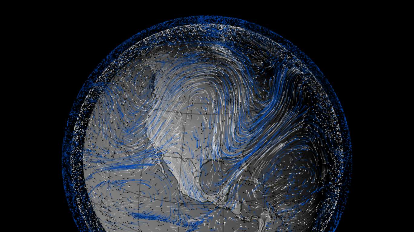
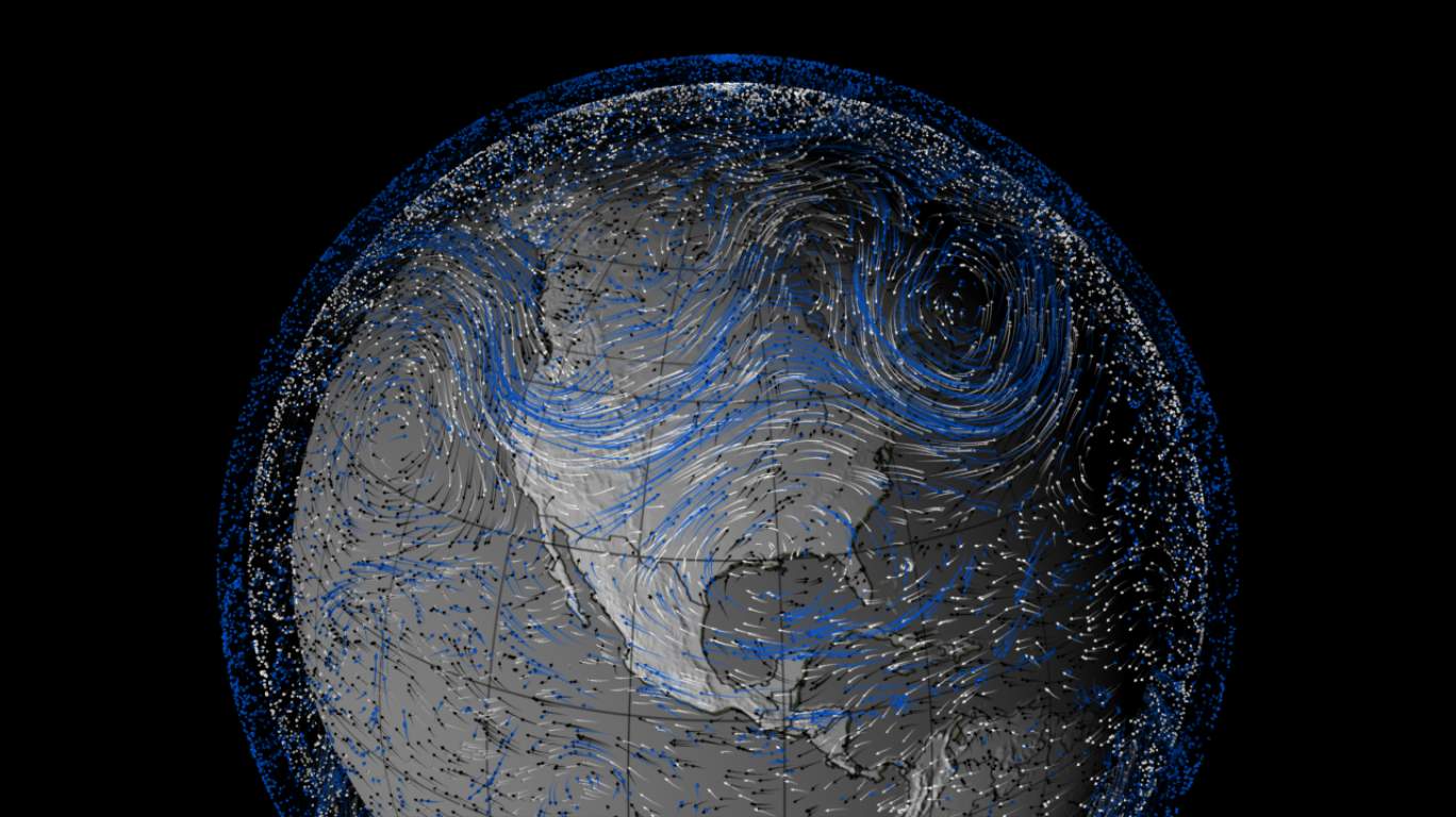
Figure 2: Wind velocity fields at three different heights (black arrows at $1.5$ km; grey at $5.4$ km; and blue at $9.2$ km) reconstructed for 1988 (top) and 1993 (bottom). Evident in both figures is the mid-latitude zonal jet that flows from west to east. By contrast in the tropics the trade winds flow from east to west. Vertical as well as horizontal shear is apparent as wind speeds generally increase with altitude. High pressure over the United States in the summer of 1988, visible as geostrophic flow moving clockwise around the high plains, led to a prolonged drought. Credit: NASA / Goddard Space Flight Center Visualization Studio and NASA Earth Observatory (October 5, 2010).

The advection of air in the atmosphere, and the transport of heat along with it, may be nicely expressed in a coordinate-independent way by introducing two scalar bilinear differential operatorsRingler:2000p118 , the Jacobian $J[,~{}]$ and flux-divergence $F[,~{}]$:

$$J[A,~{}B] \equiv \hat{r}\cdot(\vec{\nabla}A\times\vec{\nabla}B)$$

$$F[A,~{}B] \equiv \vec{\nabla}\cdot(A\vec{\nabla}B)\$$ (3)

where the derivatives act in the horizontal directions only. It is also convenient to decompose fields in the two layers into symmetric or barotropic $\overline{A}\equiv\frac{1}{2}(A_{1}+A_{0})$ and antisymmetric or baroclinic $\widehat{A}\equiv\frac{1}{2}(A_{1}-A_{0})$ modes. Thus the barotropic and baroclinic components of the bilinear field $AB$ are given by:

$$\overline{AB} = \overline{A}~{}\overline{B}+\widehat{A}~{}\widehat{B}$$

$$\widehat{AB} = \widehat{A}~{}\overline{B}+\overline{A}~{}\widehat{B}\ .$$ (4)

The barotropic divergence $\overline{\delta}=0$ in the model because any air leaving one layer enters the other. In the absence of any forcing or damping the equations of motion for the scalar fields in the two layers are:

$$\dot{\overline{q}} = J[\overline{q},~{}\overline{\psi}]+J[\widehat{q},~{}\widehat{\psi}]-F[\widehat{q},~{}\widehat{\chi}]-J[\widehat{\delta},~{}\widehat{\chi}]-F[\widehat{\delta},~{}\widehat{\psi}]$$

$$\dot{\widehat{q}} = J[\widehat{q},~{}\overline{\psi}]+J[\overline{q},~{}\widehat{\psi}]-F[\overline{q},~{}\widehat{\chi}]$$

$$\dot{\widehat{\delta}} = J[\overline{q},~{}\widehat{\chi}]+F[\widehat{q},~{}\overline{\psi}]+F[\overline{q},~{}\widehat{\psi}]-\nabla^{2}(\widehat{K}+C_{p}B\overline{\theta})$$

$$\dot{\overline{\theta}} = J[\overline{\theta},~{}\overline{\psi}]+J[\widehat{\theta},~{}\widehat{\psi}]-F(\widehat{\theta},\widehat{\chi})$$

$$\dot{\widehat{\theta}} = J[\widehat{\theta},~{}\overline{\psi}]+J[\overline{\theta},~{}\widehat{\psi}]-F(\overline{\theta},\widehat{\chi})+\overline{\theta}\widehat{\delta}$$ (5)

The first three equations describe the atmospheric flow in the two layers, driven by differences in temperature, and hence pressure, and deflected by the Coriolis force. The last two equations for the mean potential temperature $\overline{\theta}$ and static stability $\widehat{\theta}$ describe the transport of heat by the flow. $K(\psi,\chi)=\frac{1}{2}[F(\psi,\psi)-\psi\nabla^{2}\psi+F(\chi,\chi)-\chi\nabla^{2}\chi]+J[\psi,\chi]$ is the kinetic energy density per unit mass density, $C_{p}$ is the (constant pressure) specific heat of dry air and $B\equiv\frac{1}{2a^{2}}~{}[(\frac{3}{4})^{R/C_{p}}-(\frac{1}{4})^{R/C_{p}}]$ where the adiabatic exponent $R/C_{p}=\frac{2}{7}$ for ideal diatomic gases, and $a$ is the planetary radius. The equations of motion, Eq. 5, are quadratically nonlinear. As it stands they conserve total angular momentum, mean potential temperature, circulation, total energy

$$E=\int\bigg{\{}\overline{K}+\widehat{K}-C_{p}B~{}\widehat{\theta}\bigg{\}}~{}d^{2}\Omega~{},$$ (6)

and the mean square potential temperature.

The simplest way to model the effects of solar radiation and long-wave emission is by relaxing the potential temperature towards a prescribed meridional profile. To the two equations in Eqs. 5 for $\theta$ the following terms are added:

$$\dot{\overline{\theta}} = \ldots+(\overline{\theta}_{0}-\overline{\theta})/\tau_{R}$$

$$\dot{\widehat{\theta}} = \ldots+(\widehat{\theta}_{0}-\widehat{\theta})/\tau_{R}$$ (7)

where $\tau_{R}\approx 30$ days is a typical timescale for the radiative heating and cooling of the atmosphere. Prescribed functions of latitude $\overline{\theta}_{0}(\phi)=\overline{\theta}_{0}\times(\frac{1}{3}-\sin^{2}\phi)$ and $\widehat{\theta}_{0}(\phi)=\widehat{\theta}_{0}\times\cos^{2}\phi$ approximate the radiative drivingHeld:1994p409 . Energy so input is then removed through frictional coupling of the lower layer to the surface, parameterized most simply by adding damping terms to the first three mechanical equations of motion in Eq. 5: $\dot{\overline{q}}=\dots-\kappa(\overline{q}-\widehat{q})$, $\dot{\widehat{q}}=\dots-\kappa(\widehat{q}-\overline{q})$, and $\dot{\widehat{\delta}}=\dots-\kappa\widehat{\delta}$. Because the dimensionless Reynolds number $R_{e}\equiv VL/\nu$ is extremely large for large-scale atmospheric motion, viscous dissipation can be ignored.

III.2 Single Layer Model

A further simplification is possible, the reduction of the two layers to just one. In this barotropic limit pressure is a function only of density, and not of temperature, and there is no variation of the fluid motion with height. Setting $\overline{\theta}=const$ and $\widehat{\theta}=0$ in Eqs. 5 yields height-independent solutions for which the baroclinic modes have no amplitude, $\widehat{\delta}=\widehat{q}=0$. The fluid then satisfies the single-layer barotropic vorticity equation:

$$\dot{q}=J[q,\psi]$$ (8)

or equivalently

$$\frac{Dq}{Dt}\equiv\frac{dq}{dt}+\vec{v}\cdot\vec{\nabla}q=0$$ (9)

with $\overline{q}$ now written as simply $q$. As it stands this equation means that absolute vorticity is conserved under advection. Various linear forcing and damping terms can then be added to the right hand side of Eq. 9 to enable the investigation of various simple fluid models such as those described in Section IV and Subsection V.1 below.

IV Near Equilibrium Fluids

Two-dimensional turbulent flows organize spontaneously into large-scale and long-lived coherent structures, such as those seen in Fig. 3. In this DNS calculation Eq. 8 on the unit sphere has been integrated forward in time starting from an initial condition with a random pattern of vorticity (upper left panel) until only zonal jet streams, signaled by bands of vorticity of alternating sign, and a single vortex remain. The coherent structures that condense out of such freely decaying turbulence are different than those generated in a model with stochastic stirring and dampingTakehiro:2007p577 ; Obuse:2010p578 that only forms jets. As a technical necessity, both here and in the two-layer model analyzed later, an artificial viscosity called “hyperviscosity,” $\nu_{2}$, has been added to the equation of motion:

$$\dot{q}=J[q,\psi]-\nu_{2}\nabla^{2}(\nabla^{2}+2)\zeta$$ (10)

Hyperviscosity differs from the usual physical viscosity term, $\nu\nabla^{2}\zeta$, in having two more spatial derivatives. Its presence signals a fundamental limitation of all numerical simulation of low viscosity fluids: Fluctuations in the vorticity cascade down to smaller and smaller length scales, eventually dropping below the resolution of any numerical grid. Hyperviscosity is a crude statistical model for the missing sub-grid scale physics, serving to absorb fluctuations only at the small length scales while at the same time hardly disturbing the total kinetic energy of the flow. Hyperviscosity should also conserve angular momentum, and this accounts for the appearance of the $(\nabla^{2}+2)$ term that projects out the 3 modes with spherical wavenumber $\ell=1$ that contain angular momentum. This is a simple example of the dynamical protection of a conserved quantity.

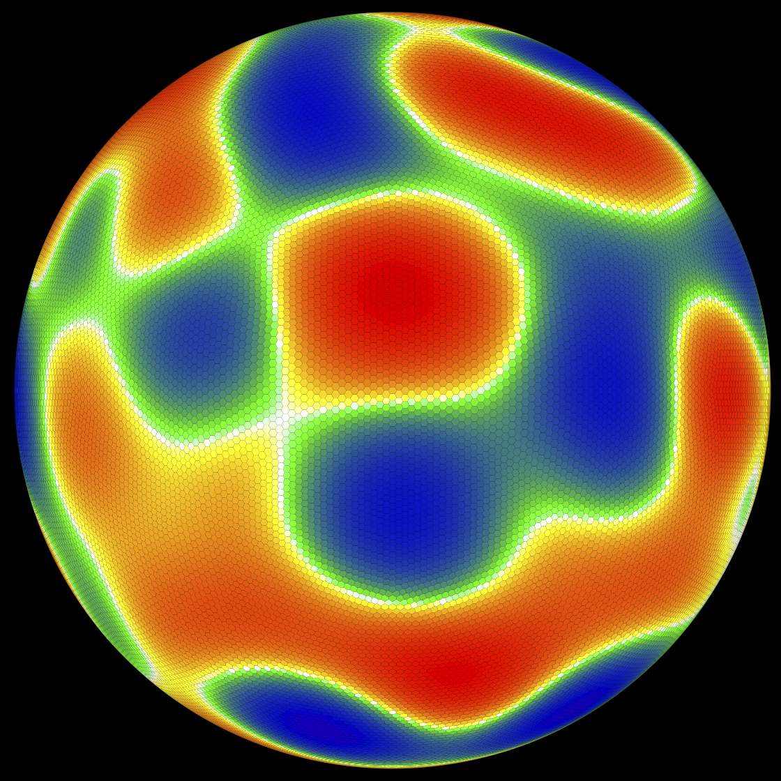
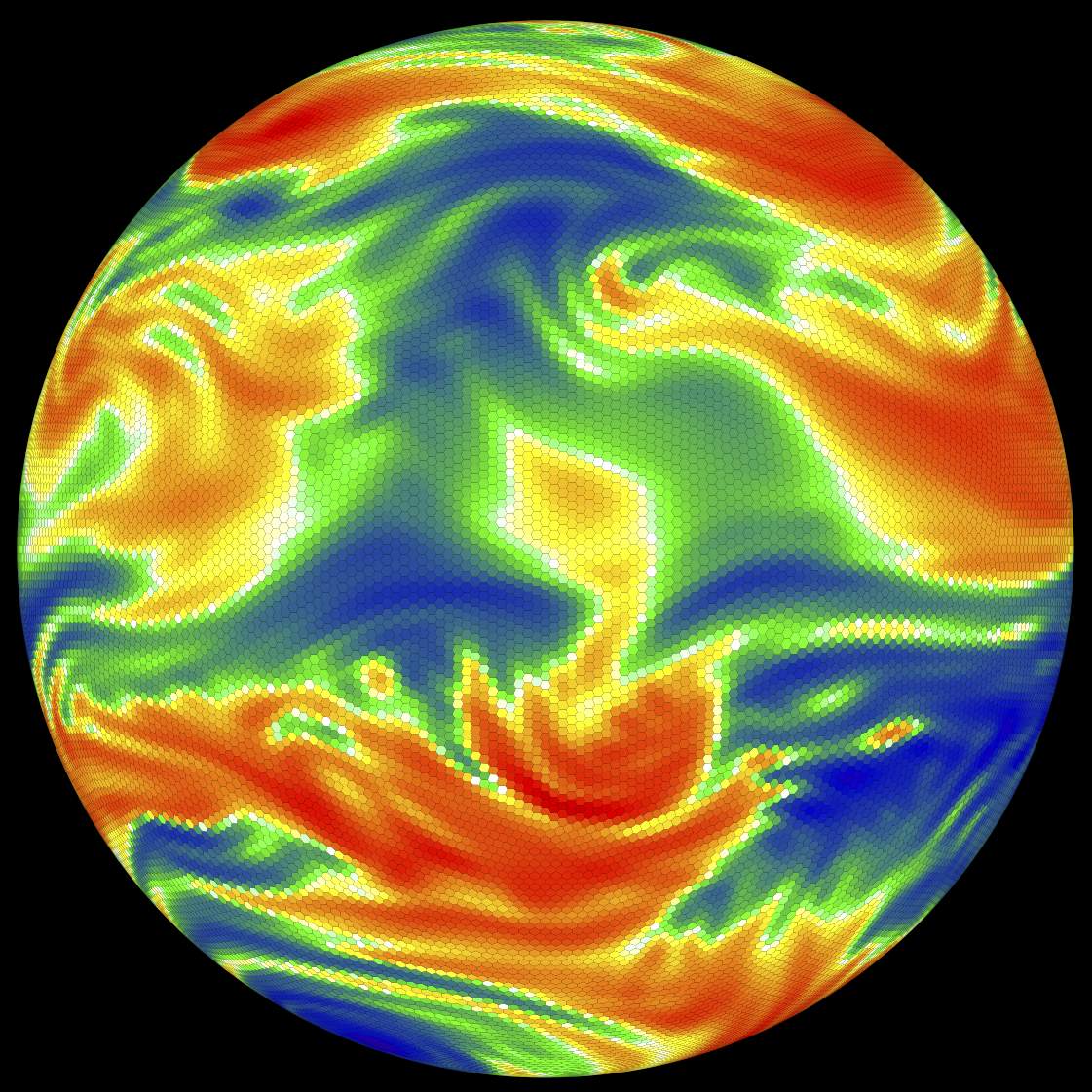
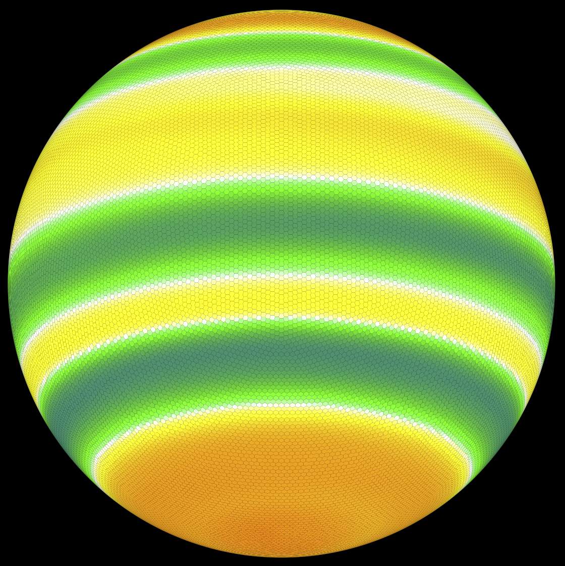
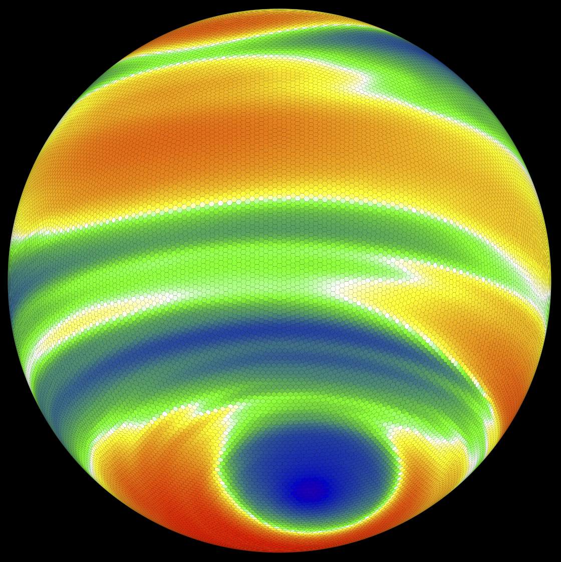
Figure 3: Time evolution of unforced relative vorticity on a sphere rotating once per day, damped only by hyperviscosity, as viewed from a point directly above a latitude of $15^{\circ}$ S. The eddy turnover time is approximately $1$ day. Clockwise from upper left: $t=0$ days, $33.7$ days, $260.8$ days, and time-averaged vorticity. The flow first develops fine structures due to nonlinear advection. It evolves at long times into a mixture of zonal jets and an isolated vortex in the southern hemisphere. The time-averaged vorticity shows the expected recovery of azimuthal symmetry in the statistic. The direct numerical simulation here is performed on a spherical geodesic gridRandall:2002p119 with $40,962$ cells. In the figure, and those that follow, the unit of time is 1 day, and the unit of distance is 1 planetary radius.

The condensation of vorticity into coherent structures (jets and vortices) occurs regardless of the detailed initial conditions, suggesting a simple variational interpretation. The simplest interpretation is based upon a principle of minimum enstrophy (ME) as developed by Bretherton and HaidvogelBretherton:1976p593 and by LeithLeith:1984p594 . Enstrophy is the mean square vorticity,

$$\frac{1}{2}~{}\int q^{2}~{}d^{2}\Omega~{},$$ (11)

and it (along with an infinite number of higher moments) is conserved in the absence of forcing or dissipation. Hyperviscosity, however, drives enstrophy towards zero faster than the kinetic energy and this separation of time scales means that effectively an equilibrium state of well-defined energy can be reached. This phenomenological approach captures in an intuitive fashion the physics of the inverse cascade processbatchelor ; Kraichnan:1980p227 whereby small-scale fluctuations organize into large-scale coherent structures.

More rigorous statistical mechanical formulations have also been constructed to describe fluids in the limit of zero viscosity. In such inviscid flows, finer and finer structures in the scalar vorticity field $\zeta(\vec{r})$ appear as the fluid evolves. Miller and collaboratorsMiller90 ; Miller:1992p122 and Robert and SommeriaRobert91 (MRS) described the small-scale fluctuations of the fluid statistically using a local probability distribution $\rho(\vec{r},\sigma)$ of vorticity $\sigma$ over a small region of space centered at $\vec{r}$. The equilibrium state is then obtained by maximizing the Boltzmann entropy while conserving energy and the infinite number of other conserved quantities, namely the moments of the vorticity distribution. In the physical limit of small but non-zero dissipation, MRS argued that the vorticity field is adequately captured by the coarse-grained mean field

$$\bar{\zeta}(\vec{r})=\int\sigma\rho(\vec{r},\sigma)~{}d\sigma$$ (12)

of the corresponding zero-viscosity theory, with dissipation acting to smooth out the small-scale structures.

However, that treatment of dissipation is unsatisfactory, because during the relaxation to equilibrium, viscosity can significantly alter the integrals of motion, especially the high-order moments. Naso, Chavanis and Dubrullenaso:2010p467 showed that maximizing the MRS entropy holding only the energy, circulation, and enstrophy fixed is equivalent to minimizing the coarse-grained enstrophy as in the earlier ME theory. The result uses the statistical MRS theory to justify the intuitive ME variational principle. There is another problem with the statistical approach, however: Figure 3 shows that even at late times the state retains some memory of the initial condition. For instance there is an isolated vortex in the southern hemisphere (somewhat like Jupiter with its Great Red Spot and jetscho1996 ) and it remains there under further time integration. The final state is determined by more than just the energy, the axial component of the angular momentum, and enstrophy.

WeichmanWeichman:2001 ; weichman05 , Majda and Wangmajda06 , and Bouchet and his collaboratorsVenaille:2009p134 ; Bouchet:2010p364 ; Venaille:2010p513 ; Venaille:2010p514 ; Bouchet:2011p535 , have applied these ideas to single-layer models of geophysical flows such as Eq. 8, finding a variety of coherent structures that switch between unidirectional jets and dipolar patterns, mimicking behavior observed in the seas. (However Balk and co-workers have argued that an additional approximate invariant is an important ingredient in jet formationBalk:2011p580 ; Nazarenko:2009p133 .) Verkley and Lynch have incorporated additional constraints and topographyVerkley:2009p238 . Near-equilibrium statistical descriptions of this type may be more applicable to oceans than to atmospheres because, as argued below, processes other than the inverse cascade are responsible for the formation of coherent structures in the atmosphere.

V Non-Equilibrium Physics By Direct Statistical Simulation

Inhomogeneous and anisotropic fluid flows pervade the universe. From the jets and vortices in the atmospheres of the outer planets, to the differential rotation of the Sun, to the large-scale circulation of the Earth’s atmosphere and oceans it is evident that such patterns of macroturbulence are the norm rather than the exception. While anisotropy and inhomogeneity pose technical difficulties when it comes to mathematical descriptions, such flows appear to be amenable to DSS, because they provide the starting point for a perturbative expansion in fluctuations, as shown below. DSS is able to reproduce statistics obtained by the traditional route of time averaging DNSlorenz67 . DSS has several advantages over DNS: (i) Low-order statistics are smoother in space and stiffer in time than the underlying detailed flows. Stationary fixed points or slowly varying statistics can therefore be described with reduced degrees of freedom and can also be accessed rapidly. (ii) Convergence with increasing resolution can be demonstrated, and for models with no subgrid physics, obviates the need for separate closure models for unresolved processes. Models with subgrid parameterizations are more naturally incorporated into DSS than DNS, because parameterizations are already inherently statistical. (iii) Finally and most importantly, DSS leads more directly to insights, by integrating out fast modes, leaving only the slow modes that contain the most interesting information. This makes the approach ideal for simulating and understanding decadal modes of the climate system, including changes in these modes that are driven by climate change. The simplest non-trivial DSS is based upon a second-order cumulant expansion that can be improved systematicallyMarston:2008p1 ; Tobias:2011p550 . Some related approaches can be found in Refs. Canuto:1994p487, ; Canuto:2001p488, . The Stochastic Structural Stability Theory (SSST) approach of Farrell and IoannouFarrell:2007p611 ; Farrell:2009p237 ; Farrell:2009p636 ; Bernstein:2010p215 in particular is closely related to the cumulant expansion truncated at second order (CE2) discussed below.

One way to formulate the direct statistical approach is by Reynolds decomposing dynamical variables $q_{i}$ such as the vorticity into the sum of a mean value and a fluctuation (or eddy):

$$q_{i}=\langle q_{i}\rangle+q_{i}^{\prime}\ \ {\rm with}~{}\langle q_{i}^{\prime}\rangle=0$$ (13)

where the choice of the averaging operation, denoted by angular brackets $\langle\rangle$, depends on the symmetries of the problem. Typical choices are time averages, or averages in the longitudinal direction (zonal averages), or averages over an ensemble of initial conditions. The first two equal-time cumulants $c_{i}$ and $c_{ij}$ of a dynamical field $q_{i}$ are defined by:

$$c_{i} \equiv \langle q_{i}\rangle$$

$$c_{ij} \equiv \langle q_{i}^{\prime}q_{j}^{\prime}\rangle=\langle q_{i}q_{j}\rangle-\langle q_{i}\rangle\langle q_{j}\rangle$$ (14)

where the second cumulant contains information about correlations that are non-local in space, correlations that are called “teleconnection patterns” in the climate literature.

The models discussed here are members of a general class of quadratically non-linear systems that may be represented with coordinate-independent equation of motion:

$$\dot{q}_{i} = A_{i}+B_{ij}~{}q_{j}+C_{ijk}~{}q_{j}q_{k}\ .$$ (15)

Latin indices $i,~{}j,~{}k$ label coordinates that may represent discrete real-space points, modes in the space of spherical harmonics, or some other alternative basis. The choice of an appropriate basis is of course of great practical importance in any actual calculation, just as for traditional condensed matter systems. There is an implicit sum over repeated indices.

The equations of motion for the cumulants can be obtained directly by differentiating Eqs. 14 with respect to time and using Eqs. 15, or non-perturbatively by introducing variables $p_{i}$ that are conjugate to the $q_{i}$ and defining the Hopf generating functionalfrisch95 ; ma:2005p108 :

$$\Psi[q(t),~{}p] \equiv e^{ip_{i}q_{i}(t)}\ .$$ (16)

The Hopf functional obeys a many-body Schrödinger-like equation:

$$i\frac{\partial}{\partial t}\Psi = \hat{H}\Psi$$ (17)

with linear operator $\hat{H}$ given by:

$$\hat{H} \equiv p_{i}\left(-A_{i}+iB_{ij}~{}\frac{\partial}{\partial p_{j}}+C_{ijk}\frac{\partial^{2}}{\partial p_{j}\partial p_{k}}\right)$$ (18)

as can be verified by combining Eqs. 16, 17, and 18 to reproduce Eq. 15. As Eq. 17 is linear in $\Psi$, the average $\overline{\Psi}\equiv\langle\Psi[q(t),~{}p]\rangle$ obeys the same equation; however $\overline{\Psi}$ now encapsulates information about the equal-time moments, as can be seen by repeated differentiation of Eq. 16 with respect to $p_{i}$, followed by averaging:

$$\langle q_{i_{1}}q_{i_{2}}\cdots q_{i_{n}}\rangle=(-i)^{n}~{}\frac{\partial^{n}\overline{\Psi}}{\partial p_{i_{1}}\partial p_{i_{2}}\cdots\partial p_{i_{n}}}\bigg{|}_{p_{i}=0}\ .$$ (19)

The Hopf functional $\overline{\Psi}$ may also be expressed as the exponential of a power series in $p_{i}$, the coefficients being the cumulants:

$$\overline{\Psi}=\exp\left\{ic_{i}(t)~{}p_{i}-\frac{1}{2!}c_{ij}(t)~{}p_{i}p_{j}-\frac{i}{3!}c_{ijk}(t)~{}p_{i}p_{j}p_{k}+\ldots\right\}$$ (20)

as can be checked by use of Eq. 19 to reproduces the moments in terms of the cumulants, Eqs. 14. Upon substituting Eq. 20 into Eq. 17 and collecting powers of $p_{i}$ one obtains equations of motion for the cumulants that through third order read:

$$\dot{c}_{i} = A_{i}+B_{ij}~{}c_{j}+C_{ijk}~{}(c_{j}~{}c_{k}+c_{jk})$$

$$\dot{c}_{ij} = \{2B_{ik}~{}c_{kj}+C_{ik\ell}~{}(4c_{\ell}~{}c_{jk}+2c_{jk\ell})\}$$

$$\dot{c}_{ijk} = \{3B_{i\ell}~{}c_{\ell jk}+6C_{k\ell m}~{}(c_{ijm}~{}c_{\ell}+c_{im}~{}c_{j\ell})\}-\mu~{}c_{ijk}+{\cal O}(c_{ijk\ell})\ .$$ (21)

Here for compactness the short-hand notation $\{\}$ has been used to denote symmetrization over indices. For example:

$$\{2B_{ik}~{}c_{kj}\}\equiv B_{ik}~{}c_{kj}+B_{jk}~{}c_{ki}$$ (22)

maintains the symmetry $\dot{c}_{ij}=\dot{c}_{ji}$.

Processes involving the non-linear term $C_{ijk}$ in Equations 21 can be visualized diagrammatically. The term $C_{ijk}~{}c_{jk}$ in the first of the equations represents the contributions of eddies to the mean flow known as Reynolds forcing (Figure 4 (b)). Scattering of an eddy by the mean flow is captured by the term $4~{}C_{ik\ell}~{}c_{\ell}~{}c_{jk}$ in the second equation and is depicted by Figure 4 (a). Finally, eddy-eddy scattering occurs only at CE3 and higher levels (the term $6~{}C_{k\ell m}~{}c_{im}~{}c_{j\ell}$ in the last of Equations 21 that is represented by Figure 4 (c)).

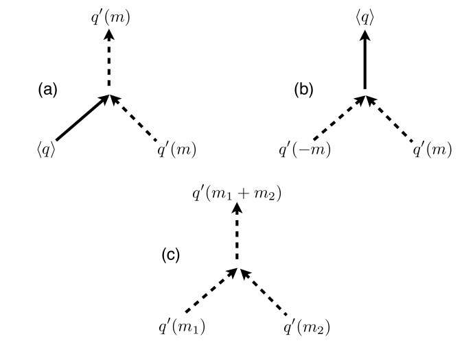
Figure 4: Eddy-mean flow and eddy-eddy triad interactions. (a) An eddy of zonal wavenumber $m\neq 0$ scatters off the mean flow. (b) Two eddies of equal but opposite zonal wavenumber combine to alter the mean flow. This is the Reynolds forcing. (c) The eddy-eddy interaction, neglected at level CE2, is included at levels CE3 and higher.

Truncated at second-order (CE2) the cumulant expansion is realizablesalmon98 (CE2 can be viewed as the exact solution of a stochastically-driven linear model) and well-behaved in the sense that the energy density is positive and the second cumulant obeys positivity constraints. The closure amounts to the neglect of eddy-eddy interactionsBernstein:2010p215 ; Tobias:2011p550 . CE2 retains the eddy-mean flow interaction. Two eddies of equal but opposite zonal wavevectors can also combine to alter the mean-flow by the Reynolds mechanism. Mathematically CE2 amounts to the assumption that the probability distribution function is adequately described by a normal, or Gaussian, distribution. Cumulant expansions are known to fail badly for the difficult problem of homogeneous, isotropic, 3D turbulencefrisch95 . In the case of anisotropic and inhomogeneous geophysical flows, however, even approximations at the CE2 level can do a surprisingly good job of describing the large-scale circulation qualitatively. Closing the equations of motion at third-order (CE3) and beyond introduces theoretical difficulties. For instance a phenomenological eddy-damping parameterOrszag:1977 ; Andre:1974p398 $\mu$ that models the neglect of the fourth and higher cumulants from the hierarchy has been included in the last of Eq. 21 and is needed to prevent the time-evolution of the cumulants from diverging. In practice, however, the statistics are insensitive to the value of $\mu$ and as shown below CE3 can improve the quantitative agreement with DNS, and even repair qualitative problems with CE2. In the absence of forcing and dissipation, both CE2 and CE3 conserve the same quantities as DNS: angular momentum, mean potential temperature, total energy, and mean-square potential temperature. Thus systematic expansions in the retained cumulants yield conserving approximations, a highly desirable trait as these help to protect against pathologies introduced by the truncation.

Still unsolved is the problem of how to systematically treat non-linearities that are not low-order polynomials (Eq. 15), such as the non-linearity due to latent heat release that is described by a step-function. Such non-linearities can be incorporated at the CE2 level by using the fact that the probability distribution function is a GaussianOGorman:2006p436 but it is not clear how to go beyond CE2. As nonlinearities more complicated than quadratic ones appear in parameterizations of boundary layers, convection, and radiation, this is an important open question that needs addressing.

V.1 Relaxation to a Prescribed Jet

The efficaciousness of DSS by expansions in cumulants can be illustrated by a simple single-layer model of barotropic flow coupled to an underlying prescribed point jet, a classic prototypical systemlindzen83 ; Nielsen84 ; schoeberl84 ; shepherd:1988p548 . The equation of motion is:

$${{\partial q}\over{\partial t}}+J[\psi,q]=\frac{q_{\rm jet}-q}{\tau}\ .$$ (23)

Forcing and dissipation are represented by the term on the right-hand-side of Eq. (23), which linearly relaxes the absolute vorticity $q$ to that of a prescribed zonal jet $q_{\rm jet}$ over a relaxation time a $\tau$. The prescribed jet is symmetric about the equator, with retrograde (east to west) velocity peaking at the equator. Such flow is described by constant relative vorticities $\pm\Gamma$ on the flanks far away from the apex and by a rounding width $\Delta\phi$ of the apex,

$$q_{\rm jet}(\phi)=f(\phi)-\Gamma\tanh\left(\frac{\phi}{\Delta\phi}\right)\$$ (24)

and appears as the dashed line in Fig. 5. Flow coupled to the jet becomes unstable and turbulent at sufficiently large values of $\tau$. As shown in Fig. 5 the absolute vorticity mixes in the equatorial region, flattening out the profile, an effect that is qualitatively captured by CE2Marston:2008p1 . However CE2 overestimates the degree of mixing; by contrast CE3 matches statistics accumulated by DNS rather well quantitatively. Examination of the second cumulant two-point correlation function (Figure 6) shows that while CE2 now fails even qualitatively to describe the statistics as determined by DNS, CE3 does rather well. The eddy-eddy interaction retained within CE3 mixes modes with different zonal wavenumbers. Wavenumbers $2$ and $3$ dominate, yielding a pattern similar to the one seen in DNS.

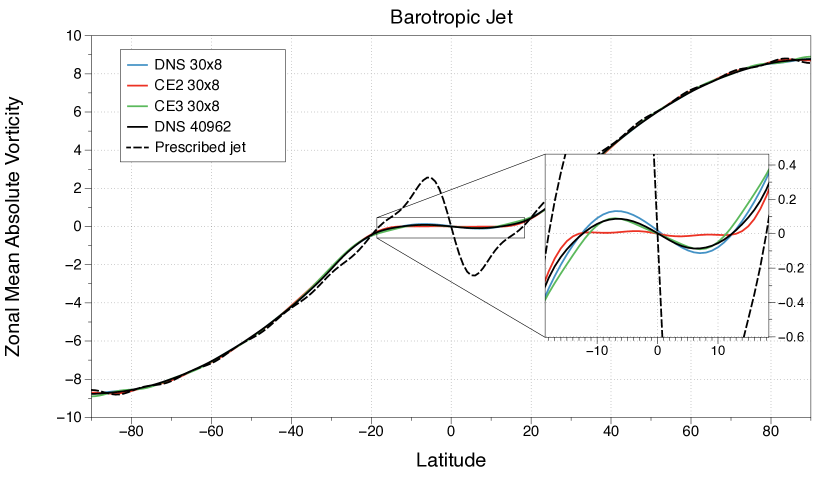
Figure 5: Zonal mean absolute vorticity of the barotropic jet as accumulated by DNS in spectral space (truncated to modes with $\ell\leq 30$ and $m\leq 8$) and compared to DSS by second- and third-order cumulant expansions (CE2 and CE3) with the same spectral resolution. Turbulence in the mixing region around the equator flattens the mean vorticity profile away from that of the prescribed jet $q_{\rm jet}$ (dashed line). The rotation period is one day ($\Omega=2\pi/$ day), $\Gamma=0.6\Omega$, $\Delta\phi=0.05$ and $\tau=50$ days (see Equations 23 and 24). Also shown for comparison are statistics accumulated from DNS on a spherical geodesic grid with $40,962$ cells, demonstrating that the spectral truncation employed here is not a severe approximation.

The eddy diffusivity finds is negative in some regions of the jet, both in DNS and in the cumulant expansionsMarston:2008p1 . This demonstrates that naive (but common) closures that replace non-linear advection with local linear diffusion must break down.

Stratification and shearing act together to weaken the nonlinearities in large-scale flows by pulling apart vorticity before it can accumulate into highly nonlinear eddies. At the same time the eddies act collectively back upon the mean-flow by the Reynolds forcing mechanism, altering itTobias:2011p550 . It is these features of the general circulation that distinguish it from the highly nonlinear problem of 3D isotropic and homogenous turbulenceSchneider2006 and make viable a systematic perturbative expansion in fluctuations about the mean-flow.

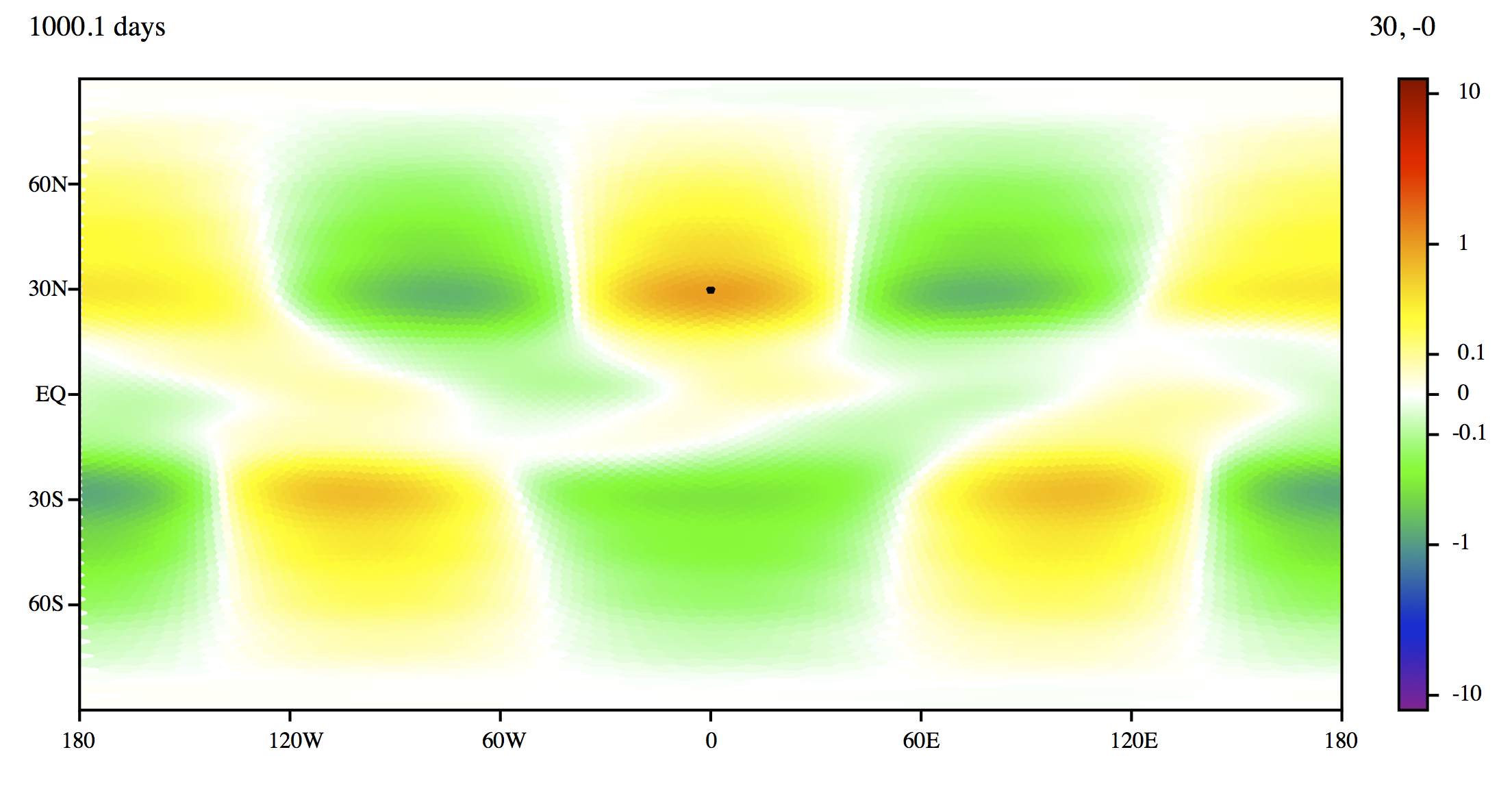
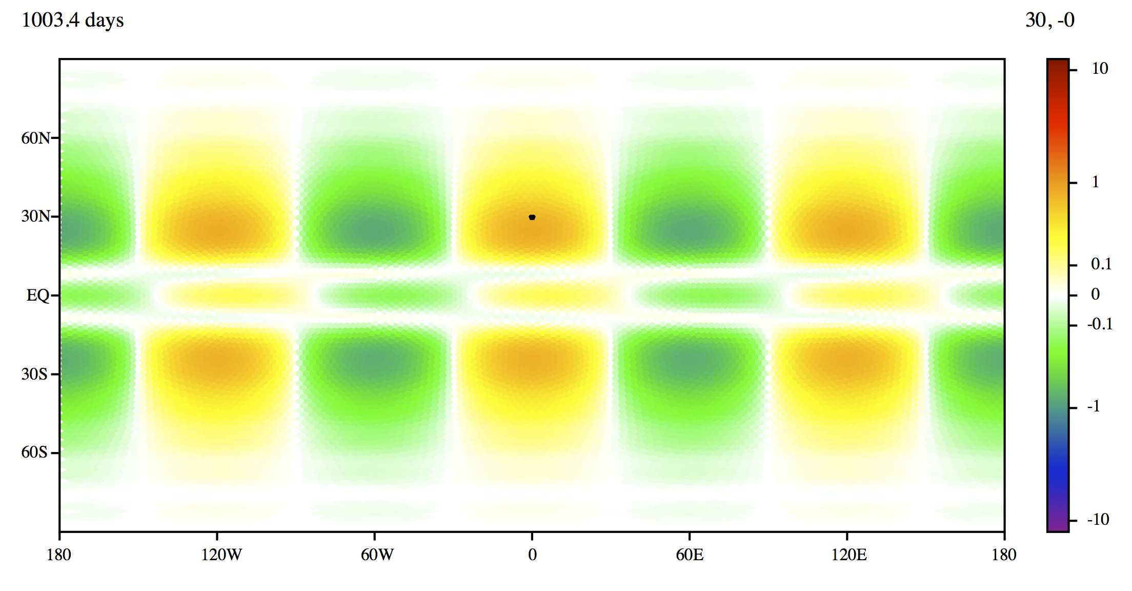
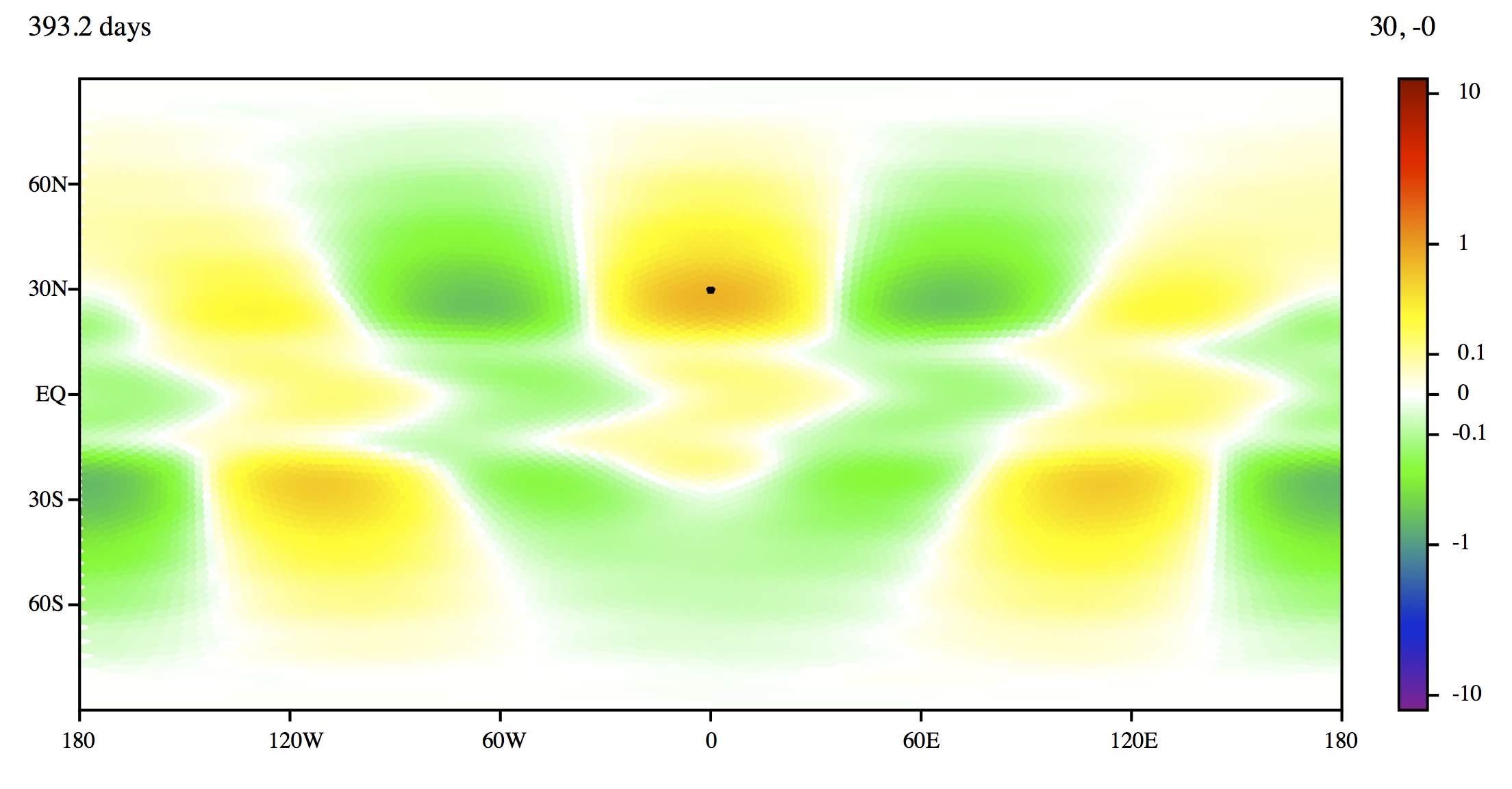
Figure 6: Second cumulant of vorticity as calculated by DNS (top), CE2 (middle) and CE3 (bottom). The two-point correlations are with respect to a reference point at a latitude of $30^{\circ}$ and along the prime meridian marked by the black dot. The correlations show that the dominant fluctuations have zonal wavenumbers $2$ and $3$. CE2, however, only exhibits fluctuations at wavenumber $3$. This defect is repaired at the CE3 level.

V.2 Two Layer Primitive Equation Model

A qualitatively realistic model of the general circulation, at least for regions outside of the tropics that are dominated by convection, is provided by the two layer primitive equation model introduced in subsection III.1. As shown in Figure 7 the model develops midlatitude westerly jets and storm tracks, as well as easterly trade winds in the tropics. Hadley cells with overturning circulation near $\pm 30^{\circ}$ latitude mimic those of Earth. Zonal means determined by CE2 agree qualitatively with DNS, but as Figure 8 shows, there are quantitative discrepancies in the zonal winds, especially at high latitudes.

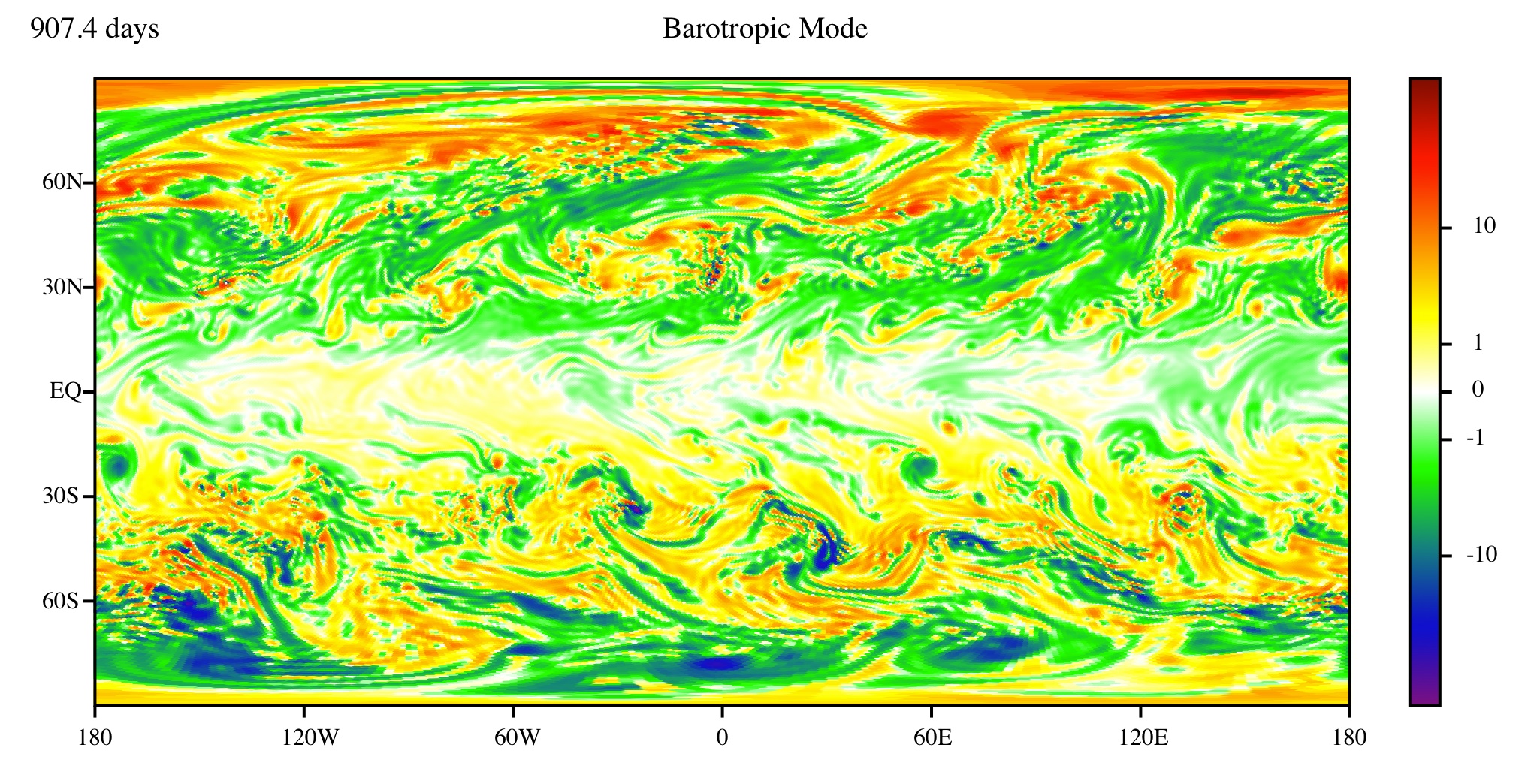
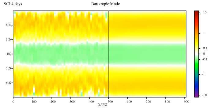
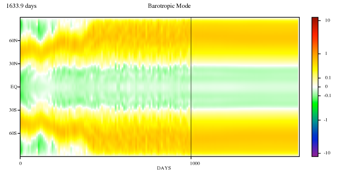
Figure 7: Top: Snapshot of the barotropic vorticity as calculated by DNS on a spherical geodesic grid of $163,842$ cells. Here the rotation period is one day, $a=1$ Earth radius, $\tau_{R}=33$ days, $1/\kappa=10$ days, the barotropic potential temperature relaxes to a $\overline{\theta}_{0}=120$K equator-to-pole gradient, and the baroclinic temperature relaxes to $\hat{\theta}_{0}=30$K, suppressing convection. Middle and bottom: Timelines of the mean zonal velocity, averaged over both layers, as calculated by DNS (middle panel) and by CE2 with spectral truncation $\ell\leq 50$ (bottom panel). Time averaging is turned on at the time indicated by the black vertical line, smoothing out any fluctuations that survive the zonal average. The mid-latitude westerly winds and the tropical easterlies are similar to Earth’s general circulation.

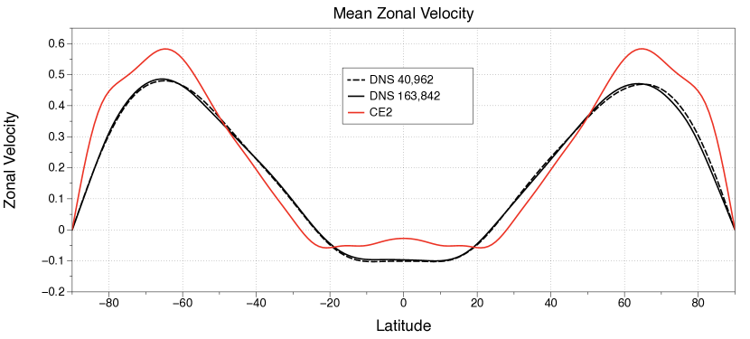
Figure 8: Mean zonal velocity, averaged over both layers, for the two-layer primitive equation as accumulated by DNS on spherical geodesic grids of two different resolutions and compared to CE2. Convergence in the statistic with increasing DNS resolution is apparent. Both DNS and CE2 reproduce midlatitude westerlies and tropical easterly winds, but CE2 only agrees with DNS at a qualitative level. Same parameters as Figure 7.

The second cumulant two-point correlation function is compared in Figure 9. Correlations are considerably shorter-ranged in DNS than in CE2, and the correlations are confined to a single hemisphere. Whether or not CE3 would address these discrepancies is an open question.

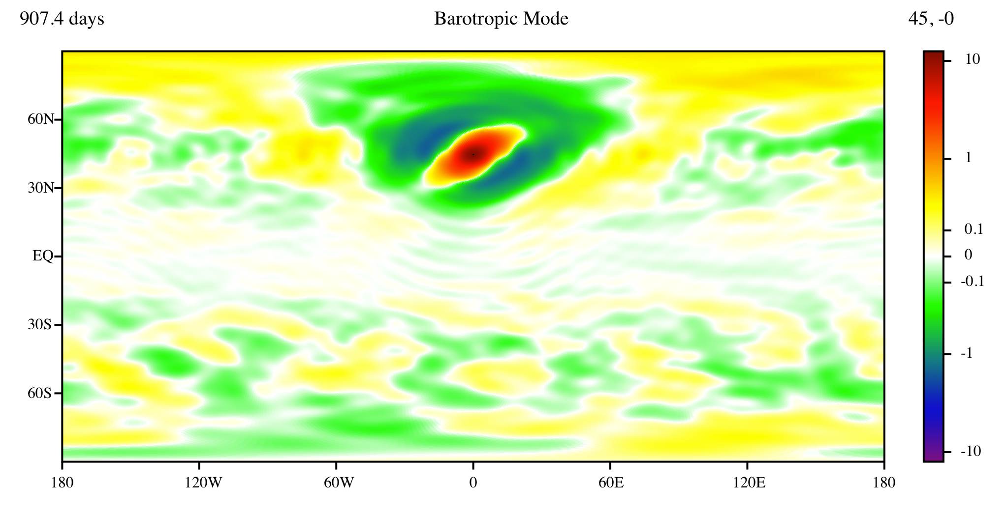
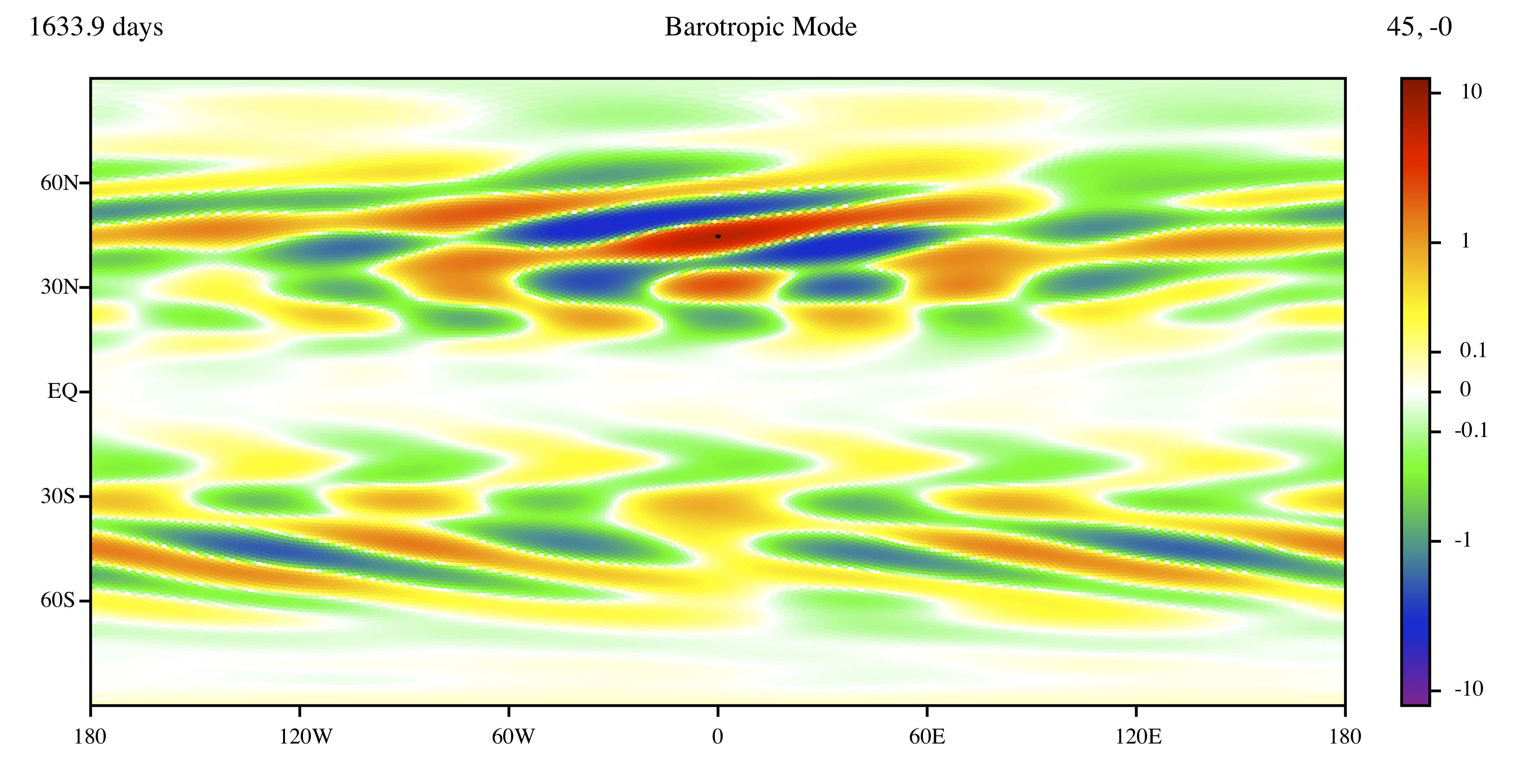
Figure 9: Second cumulant of barotropic vorticity as calculated by DNS on a spherical geodesic grid of $163,842$ cells (top) and CE2 retaining modes with $\ell\leq 50$ (bottom). The two-point correlations are with respect to a reference point near the middle of the storm track at a latitude of $45^{\circ}$ and along the prime meridian. Same parameters as Figure 7. Correlations in the flow are seen to be much shorter ranged in DNS than in CE2.

In any case, longer ranged correlations are evident both in a two-layer quasi-geostrophic modelMarston:2010 and in a multilayer modelOGorman:2007p76 so the short-ranged nature of the correlations evident here in DNS may be an artifact of the two-layer approximation.

Additional insights into the general circulation, and the formation of zonal jets, can be gained from the spectrum of kinetic energy fluctuations. In both simulations of the general circulation with and without the eddy-eddy interactionOGorman:2007p76 , and in the real atmosphereBoer1983 ; Nastrom1985 , there is a $\ell^{-3}$ power-law scaling for spherical wavenumbers $\ell$ greater than the characteristic eddy wavenumber of approximately $10$. Frequently this power-law decay is explained by invoking a cascade of enstrophy towards small scalesKraichnan:1980p227 ; salmon98 ; however no such cascade can occur in the absence of eddy-eddy interactions. Furthermore, in the real atmosphere there is no inertial range for which eddy-eddy interactions dominateOGorman:2007p76 . Rather other contributions to the spectrum stemming from the conversion of potential to kinetic energy, and friction, are importantLambert1987 ; Straus1999 , making arguments for power-law scaling that are based upon enstrophy cascades questionableVallis:1992 .

V.3 Velocity Profile of a Vortex

In the absence of the Coriolis force, large-scale vortices condense in two-dimensional flowsbatchelor ; Kraichnan:1980p227 ; cho1996 ; Chertkov:2007p589 ; Marston:2011p604 . Chertkov, Kolokolov, and LebedevChertkov:2010p588 have used an expansion similar to CE3 to study the mean radial profile of the velocity of an isolated vortex. They were able to reproduce the $r^{-\frac{1}{4}}$ power-law decrease in the velocity as a function of the distance $r$ from the vortex center seen in DNSChertkov:2007p589 . Here, as in the previous examples, the strong mean-flow around the vortex provides a basis for a perturbative expansion in fluctuations about it.

VI Other Approaches

The complexity of non-equilibrium statistical mechanics raises the question of whether or not simple principles can be found that generalize equilibrium statistical mechanics and thermodynamics to non-equilibrium systems. Two such approaches are outlined below.

VI.1 Maximum Entropy Production

A school of thought has built up around the provocative notion that a principle of maximum entropy production (MEP) offers a route to understanding systems driven away from equilibrium comparable to the Boltzmann hypothesis in equilibrium statistical mechanics. Refs. Lorenz:2003p210, ; Ozawa:2003p212, ; Kleidon:2004p208, ; Whitfield:2005p166, ; Woollings:2006p162, ; Goody:2007p163, ; Lucarini:2009p688, are a sample of recent work. An early apparent success came when Paltridge applied these ideas to simple box models of the Earth’s atmosphere. Paltridge’s model assumed that the atmosphere acts either to maximize the production of entropy, or alternatively maximize dissipation, as it transports heat poleward. Intriguingly the calculated pole-to-equator temperature difference was close to the observed difference of about 60 KPaltridge:1975 ; Paltridge:1979p470 ; Paltridge:2001 . However the planetary rotation rate does not enter the calculation – yet it certainly exerts strong control over the temperature gradient. On Earth the Coriolis force strongly deflects winds in meridional directions, inhibiting the transfer of heat out of the tropics. On a planet rotating more rapidly than Earth there should be an even larger equator-to-pole temperature gradient; conversely on a slowly rotating planet the atmosphere would efficiently redistribute heat, nearly erasing the gradient. The two-layer primitive equation model illustrates the strong dependence on the rotation rate nicely (see Figure 10). That Paltridge’s idea yielded a pole-to-equator temperature difference close to reality appears to be a coincidence.

Dewar has attempted to ground MEP in more fundamental principlesDewar:2003p207 ; Lorenz:2003p210 ; Dewar:2005p211 . Dewar used the maximum information entropy approach of Jaynes (see his two 1957 papers published in Physical Review Jaynes:1957a ; Jaynes:1957b ) to generalize the equilibrium ensemble by introducing a probability measure over space-time paths taken by systems that are driven away from equilibrium. However a number of problems with Dewar’s theory have been discussed in the literatureGrinstein:2007p419 ; Bruers:2007p457 ; Paquette:2010p520 . In particular PaquettePaquette:2010p520 considered an exactly solvable Langevin equation that describes a massive Brownian particle in a viscous medium, driven by stochastic fluctuations resulting from the impact of many light particles. He showed that the probability functional for a given particle path cannot be reproduced by application of Dewar’s frameworkDewar:2003p207 . As stochastic models are a common way to drive large-scale motion in reduced modelsChandrasekhar:1943p674 ; vandenEijnden:1998p676 , and also find increasing use in weather and climate simulations as a way to model unresolved processes such as small-scale convectionHasselmann:1976p675 ; Palmer:2010 , the failure of the Dewar formalism to yield the correct statistics raises the question of its wider applicability.

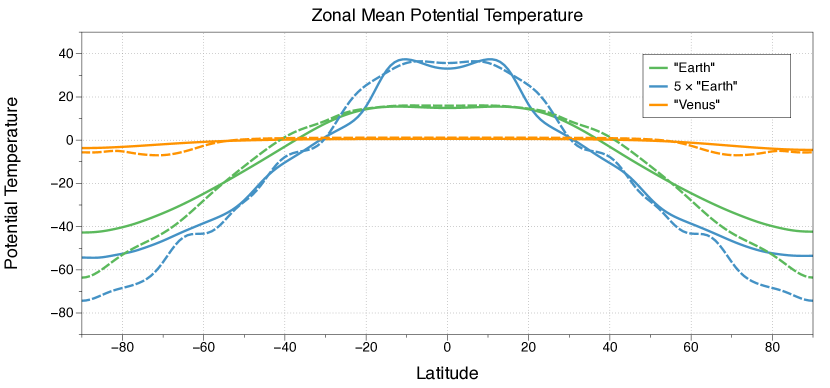
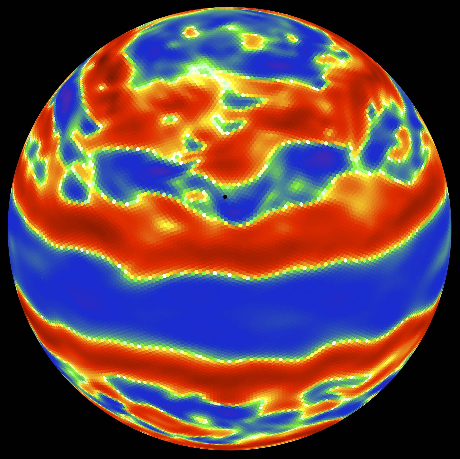
Figure 10: Top: Time and zonally averaged potential temperature as calculated by DNS (solid lines) and CE2 (dashed lines) of the two-layer primitive equation model for three planets that differ only in their rate of rotation. In each case the atmosphere relaxes to an imposed $120$ K equator-to-pole temperature difference. “Earth” rotates once per day; “Venus” has a rotation period of 100 days, and “5 $\times$ Earth” completes a rotation in 0.2 days. Bottom: A snapshot of the zonal velocity for “5 $\times$ Earth” reveals that it has two westerly jets in each hemisphere. Except for the rotation rate, the parameters are the same as Figure 7.

The two-layer model also reveals other interesting phenomena such as the spontaneous breaking of time-reversal symmetry. For a planet with no rotation, $\Omega=0$ and simulation finds no preference for the atmosphere to rotate in a particular sense. The total angular momentum of the atmosphere remains zero. A small but non-zero planetary rotation rate is enough to induce a striking superrotation of the atmosphere, with vigorous winds at all latitudes moving in the direction of planetary rotation, but moving much faster than the planet’s surface. The Hadley cells now extend over each entire hemisphere. Such superrotation has been seen in the winds of Venus and Titan.

In the opposite limit of high rotation (the $5\times$ Earth model in Figure 10) the system undergoes a phase transition with multiple westerly jets now appearing in each hemisphere. Multiple jets are also found in the atmosphere of Jupiter and can be understood in terms of the Rhines scale

$$\ell_{R} \equiv \sqrt{u_{rms}/\beta}$$ (25)

where

$$\beta \equiv \frac{df}{d(a\phi)}$$ (26)

is the gradient of the Coriolis parameter, $u_{rms}$ is the root mean square speed of the jet eddiestapio , and $a$ is the radius of the planet. The Rhines scale determines the width of the jets. Increasing $\Omega$ increases $\beta$ and makes $\ell_{R}\ll a$, permitting more than one jet to fit into each hemisphereGalperin:2007p595 . SSST is able to reproduce the linear dependence of the number of jets on the inverse Rhines scaleFarrell:2007p611 .

VI.2 Linear Response

The fluctuation-dissipation theorem relates the linear response of a system to perturbing influences to two-point correlations (the fluctuations). If generalizable to non-equilibrium systems, an obvious application would be to understand the influence of various drivers of climate change, such as rising levels of greenhouse gases, upon the climate within such a framework. The approach has been applied to highly simplified models with just a few degrees of freedomCooper:2011p640 ; KirkDavidoff:2009p629 . One lesson learned from the work of Kirk-DavidoffKirkDavidoff:2009p629 is that care must be taken when applying linear response theory to actual climate dataSchwartz:2007p616 to extract an estimate of climate sensitivity, as long time series are necessaryScafetta:2008p617 . Application of linear response theory to a full atmospheric general circulation model with many degrees of freedom has also been attempted by Gritsun, Branstator, and MajdaGritsun:2008p277 . These authors report qualitative agreement between the linear and the actual response of the model.

VII Summary and Open Questions

Viewing planetary atmospheres from the perspective of condensed matter physics provides new insights. Idealized models of atmospheres, like those of traditional condensed matter, can be understood in detail and used to explain observed phenomena such as the statistics of the general circulation. Ideas and tools discussed here may see application to both deep-time reconstructions of climate (as ESMs have difficulty simulating vast periods of time) and to newly discovered and characterized exoplanets, as well as to the present-day climate of Earth and the pressing question of climate change.

Still unclear, however, is the range of applicability of such approaches, and whether or not they can advance from being qualitative tools to become quantitatively accurate theories of the general circulation, possibly even replacing the traditional technique of direct numerical simulation. There is thus a pressing need for improved theoretical frameworks and tools to better describe non-equilibrium statistical physics. Will near-equilibrium theories prove valuable in the description of real geophysical flows? Are there reliable general principles of non-equilibrium statistical physics waiting to be discovered? Can quantitatively accurate DSS closures be found that are at the same time computationally efficient? Can non-perturbative formulations be implemented, possibly with the use of renormalization-group ideas?mccomb2004 Is it possible to extend DSS to ESMs that are complex enough to address questions such as how the storm tracks and ocean currents will shift as the climate changes?OGorman:2010p506 By thinking about atmospheres as condensed matter systems it appears possible that progress can be made on answering these important questions.

VIII Acknowledgments

I thank Freddy Bouchet, Kerry Emanuel, Grisha Falkovich, Paul Kushner, Paul O’Gorman, Glenn Paquette, Wanming Qi, Florian Sabou, Tapio Schneider, Steve Tobias, Peter Weichman, and Bill Young for helpful discussions. I would also like to thank Caltech for its hospitality during a sabbatical visit when this article was written, and Jim Langer for reading the article and offering helpful questions and suggestions. This work was supported in part by NSF grant Nos. DMR-0605619 and CCF-1048701.

IX Mini-Glossary

The following brief definitions are adapted in part from the Glossary of Meteorologyams:2000 .

1. baroclinic: The component of a field that varies with altitude.

2. barotropic: The component of a field that is uniform with altitude.

3. direct numerical simulation (DNS): Numerical simulation of equations of motion. Statistics are accumulated by sampling fields during time integration.

4. direct statistical simulation (DSS): Numerical simulation of the equations of motion for the statistics themselves.

5. eddy: The departure of a field from its zonal mean.

6. geostrophic: A balance between horizontal Coriolis and pressure forces.

7. Hadley cell: Circulating winds in the tropics that near the surface move toward the equator, rise near the equator, move poleward and then sink back towards the surface near $\pm 30^{\circ}$ latitude.

8. potential temperature: Temperature that a parcel of dry air would have if brought adiabatically from its initial state to a standard pressure.

9. superrotation: Flow along the equator in the direction of the planetary rotation.

10. zonal mean: The mean value of a field, averaged over longitude, expressed as a function of latitude.

X Important Acronyms

1. CE2: Second-order cumulant expansion.

2. CE3: Third-order cumulant expansion.

3. DNS: Direct numerical simulation.

4. DSS: Direct statistical simulation.

5. ESM: Earth system model.

6. ME: Minimum enstrophy.

7. MEP: Maximum entropy production

References

- (1) J. B. Marston. Looking for new problems to solve? Consider the climate. Physics, 4:20, 2011.
- (2) Jose Pinto Peixoto and Abraham H. Oort. Physics of Climate. American Institute of Physics, New York, 1992.
- (3) Rick Salmon. Lectures on Geophysical Fluid Dynamics. Oxford University Press, New York, 1998.
- (4) Geoffrey K Vallis. Atmospheric and Oceanic Fluid Dynamics. Cambridge University Press, 2006.
- (5) Tapio Schneider. The general circulation of the atmosphere. Annual Review of Earth and Planetary Science, 34:655 – 688, 2006.
- (6) X.-P Huang and C. F Driscoll. Relaxation of 2d turbulence to a metaequilibrium near the minimum enstrophy state. Physical Review Letters, 72:2187–2190, 1994.
- (7) Eric R Weeks, Yudong Tian, J. S Urbach, Kayo Ide, Harry L Swinney, and Michael Ghil. Transitions between blocked and zonal flows in a rotating annulus. Science, 278:1598–1601, 1997.
- (8) A. A Castrejón-Pita and P. L Read. Synchronization in a pair of thermally coupled rotating baroclinic annuli: Understanding atmospheric teleconnections in the laboratory. Phys. Rev. Lett., 104:204501, 2010.
- (9) M Shats, D Byrne, and H Xia. Turbulence decay rate as a measure of flow dimensionality. Physical Review Letters, 105:264501, 2010.
- (10) Burkhard Militzer and Hugh Wilson. New phases of water ice predicted at megabar pressures. Physical Review Letters, 105:195701, 2010.
- (11) Isaac M Held. The gap between simulation and understanding in climate modeling. Bulletin of the American Meteorological Society, 86:1609 – 1614, 2005.
- (12) Gerard Roe. Feedbacks, timescales, and seeing red. Annual Review of Earth and Planetary Sciences, 37:93–115, 2009.
- (13) DG Vaughan and R Arthern. Why is it hard to predict the future of ice sheets? Science, 315:1503–1504, 2007.
- (14) P.H Stone. The atmospheric general circulation: Some unresolved issues. Dynamics of Atmospheres and Oceans, 44:244–250, 2008.
- (15) G. L. Stephens. Cloud feedbacks in the climate system: A critical review. J. Climate, 18:237–273, 2005.
- (16) H Xia, D Byrne, G Falkovich, and M Shats. Upscale energy transfer in thick turbulent fluid layers. Nature Physics, 7:1–4, 2011.
- (17) E N Lorenz. Energy and numerical weather prediction. Tellus, XII:364–373, 960.
- (18) R Heikes and DA Randall. Numerical integration of the shallow-water equations on a twisted icosahedral part i: Basic design and results of tests. Monthly Weather Review, 123:1862 – 1880, 1995.
- (19) David J. Stendsrud. Parameterization schemes: keys to understanding numerical weather prediction models. Cambridge University Press, New York, NY, 2007.
- (20) R T Pierrehumbert. Principles of Planetary Climate. Cambridge University Press, Cambridge, UK, 2011.
- (21) IM Held and MJ Suarez. A proposal for the intercomparison of the dynamical cores of atmospheric general circulation models. Bulletin of the American Meteorological Society, 75:1825–1830, 1994.
- (22) IM Held and MJ Suarez. A two-level primitive equation atmospheric model designed for climatic sensitivity experiments. Journal of the Atmospheric Sciences, 35:206–229, 1978.
- (23) Sukyoung Lee and Isaac M Held. Baroclinic wave packets in models and observations. Journal of the Atmospheric Sciences, 50:1413–1428, 1993.
- (24) TD Ringler, RP Heikes, and DA Randall. Modeling the atmospheric general circulation using a spherical geodesic grid: A new class of dynamical cores. Monthly Weather Review, 128:2471–2490, 2000.
- (25) Shin Takehiro, Michio Yamada, and Yoshi-Yuki Hayashi. Energy accumulation in easterly circumpolar jets generated by two-dimensional barotropic decaying turbulence on a rapidly rotating sphere. Journal of the Atmospheric Sciences, 64:4084–4097, 2007.
- (26) Kiori Obuse, Shin-Ichi Takehiro, and Michio Yamada. Long-time asymptotic states of forced two-dimensional barotropic incompressible flows on a rotating sphere. Physics of Fluids, 22:056601, 2010.
- (27) DA Randall, TD Ringler, RP Heikes, P Jones, and J Baumgardner. Climate modeling with spherical geodesic grids. Computing in Science & Engineering, 4:32–41, 2002.
- (28) F. P Bretherton and D. B Haidvogel. Two-dimensional turbulence above topography. Journal of Fluid Mechanics, 78:129–154, 1976.
- (29) C. E Leith. Minimum enstrophy vortices. Physics of Fluids, 27:1388–1395, 1984.
- (30) G. K. Batchelor. Computation of the energy spectrum in homogeneous two-dimensional turbulence. Physics of Fluids, 12:II–233–II–239, 1969.
- (31) R H Kraichnan and D Montgomery. Two-dimensional turbulence. Rep. Prog. Phys., 43:547–619, 1980.
- (32) J Miller. Statistical mechanics of euler equations in two dimensions. Phys. Rev. Lett., 65:2137–2140, 1990.
- (33) J Miller, PB Weichman, and MC Cross. Statistical mechanics, euler’s equation, and jupiter’s red spot. Physical Review A, 45:2328–2359, 1992.
- (34) R Robert and J Sommeria. Statistical equilibrium states for two-dimensional flows. J. Fluid Mech., 229:291–310, 1991.
- (35) A Naso, P. H Chavanis, and B Dubrulle. Statistical mechanics of two-dimensional euler flows and minimum enstrophy states. The European Physical Journal B, 77:187–212, 2010.
- (36) James Y-K Cho and Lorenzo M Polvani. The emergence of jets and vortices in freely evolving, shallow-water turbulence on a sphere. Phys. Fluids, 8:1531–1552, 1996.
- (37) Peter B. Weichman and Dean M. Petrich. Statistical equilibrium solutions of the shallow water equations. Phys. Rev. Lett., 86(9):1761–1764, 2001.
- (38) Peter B Weichman. Equilibrium theory of coherent vortex and zonal jet formation in a system of nonlinear rossby waves. Phys. Rev. E, 73:036313, 2006.
- (39) Andrew J Majda and Xiaoming Wang. Nonlinear Dynamics and Statistical Theories for Basic Geophysical Flows. Cambridge University Press, Cambridge UK, 2006.
- (40) Antoine Venaille and Freddy Bouchet. Statistical ensemble inequivalence and bicritical points for two-dimensional flows and geophysical flows. Phys. Rev. Lett., 102:104501, 2009.
- (41) Freddy Bouchet and Marianne Corvellec. Invariant measures of the 2d Euler and Vlasov equations. J. Stat. Mech., 8:P08021, 2010.
- (42) Antoine Venaille and Freddy Bouchet. Solvable phase diagrams and ensemble inequivalence for two-dimensional and geophysical turbulent flows. J. Stat. Phys., 143:346–380, 2011.
- (43) Antoine Venaille and Freddy Bouchet. Oceanic rings and jets as statistical equilibrium states. arXiv:1011.2556 (to appear in J. Phys. Oceanogr.).
- (44) Freddy Bouchet and Antoine Venaille. Statistical mechanics of two-dimensional and geophysical flows. arXiv:1110.6245 (to appear in Physics Reports).
- (45) Alexander M Balk, Francois van Heerden, and Peter B Weichman. Rotating shallow water dynamics: Extra invariant and the formation of zonal jets. Phys. Rev. E, 83:046320, 2011.
- (46) Sergey Nazarenko and Brenda Quinn. Triple cascade behavior in quasigeostrophic and drift turbulence and generation of zonal jets. Phys. Rev. Lett., 103:118501, 2009.
- (47) WTM Verkley and P Lynch. Energy and enstrophy spectra of geostrophic turbulent flows derived from a maximum entropy principle. Journal of the Atmospheric Sciences, 66:2216–2236, 2009.
- (48) E N Lorenz. The Nature and Theory of the General Circulation of the Atmosphere, volume 218. World Meteorological Organization, Geneva Switzerland, 1967.
- (49) J B Marston, E Conover, and T Schneider. Statistics of an unstable barotropic jet from a cumulant expansion. Journal of the Atmospheric Sciences, 65:1955–1966, 2008.
- (50) S. M Tobias, K Dagon, and J. B Marston. Astrophysical fluid dynamics via direct statistical simulation. The Astrophysical Journal, 727:127, 2011.
- (51) V. M Canuto, F. O Minotti, and O Schilling. Differential rotation and turbulent convection: A new reynolds stress model and comparison with solar data. The Astrophysical Journal, 425:303–325, 1994.
- (52) V. M Canuto, Y Cheng, and A Howard. New third-order moments for the convective boundary layer. Journal of Atmospheric Sciences, 58:1169–1172, 2001.
- (53) Brian F Farrell and Petros J Ioannou. Structure and spacing of jets in barotropic turbulence. Journal of the Atmospheric Sciences, 64:3652–3665, 2007.
- (54) B F Farrell and PJ Ioannou. A theory of baroclinic turbulence. Journal of the Atmospheric Sciences, 66:2444–2454, 2009.
- (55) Brian F Farrell and Petros J Ioannou. Emergence of jets from turbulence in the shallow-water equations on an equatorial beta plane. Journal of the Atmospheric Sciences, 66:3197–3207, Oct 2009.
- (56) Joseph Bernstein and Brian Farrell. Low-frequency variability in a turbulent baroclinic jet: Eddy–mean flow interactions in a two-level model. Journal of the Atmospheric Sciences, 67:452–467, 2010.
- (57) Uriel Frisch. Turbulence: The Legacy of A. N. Kolmogorov. Cambridge University Press, Cambridge UK, 1995.
- (58) O Ma and J B Marston. Exact equal time statistics of orszag–mclaughlin dynamics investigated using the hopf characteristic functional approach. Journal of Statistical Mechanics: Theory and Experiment, 2005:P10007, 2005.
- (59) Steven A Orszag. Lectures on the statistical theory of turbulence. Fluid Dynamics, Les Houches 1973, Gordon and Breach, New York NY, 1977.
- (60) J-C Andre. Irreversible interactions between cumulants in homogeneous, isotropic, two-dimensional turbulence theory. The Physics of Fluids, 17:15–21, 1974.
- (61) Paul A O’Gorman and Tapio Schneider. Stochastic models for the kinematics of moisture transport and condensation in homogeneous turbulent flows. Journal of Atmospheric Sciences, 63:2992–3005, 2006.
- (62) R S Lindzen, A J Rosenthal, and R Farrell. Charney’s problem for baroclinic instability applied to barotropic instability. J. Atmos. Sci., 40:1029–1034, 1983.
- (63) J E Nielsen and M R Schoeberl. A numerical simulation of barotropic instability. part ii: Wave-wave interaction. J. Atmos. Sci., 41:2869–2881, 1984.
- (64) Mark R Schoeberl and Richard S Lindzen. A numerical simulation of barotropic instability. part i: Wave-mean flow interaction. J. Atmos. Sci., 41:1368–1379, 1984.
- (65) Theodore G Shepherd. Rigorous bounds on the nonlinear saturation of instabilities to parallel shear flows. Journal of Fluid Mechanics, 196:291–322, 1988.
- (66) J B Marston. Statistics of the general circulation from cumulant expansions. Chaos, 20:041107, 2010.
- (67) PA O’Gorman and T Schneider. Recovery of atmospheric flow statistics in a general circulation model without nonlinear eddy–eddy interactions. Geophys. Res. Lett, 34:524–535, 2007.
- (68) G J Boer and T G Shepherd. Large-scale two-dimensional turbulence in the atmosphere. Journal of Atmospheric Sciences, 40:164–184, 1983.
- (69) G D Nastrom and K S Gage. A climatology of atmospheric wavenumber spectra of wind and temperature observed by commerical aircraft. Journal of Atmospheric Sciences, 42:950–960, 1985.
- (70) S J Lambert. Spectral energetics of the canadian climate centre general circulation model. Monthly Weather Review, 115:1295–1304, 1987.
- (71) D M Straus and P Ditlevsen. Two-dimensional turbulence properties of the ecmwf reanalyses. Tellus A, 51:749–772, 1999.
- (72) G K Vallis. Problems and phenomenology in two-dimensional turbulence. In G F Carnevale and R T Pierrehumbert, editors, Non-linear Phenomena in Atmospheric and Oceanic Sciences, pages 1–25. Springer, New York NY, 1992.
- (73) M Chertkov, C Connaughton, I Kolokolov, and V Lebedev. Dynamics of energy condensation in two-dimensional turbulence. Physical Review Letters, 99:084501, 2007.
- (74) M Chertkov, I Kolokolov, and V Lebedev. Universal velocity profile for coherent vortices in two-dimensional turbulence. Phys. Rev. E, 81:015302, 2010.
- (75) R Lorenz. Computational mathematics: Full steam ahead-probably. Science, 299:837, 2003.
- (76) H Ozawa, A Ohmura, RD Lorenz, and T Pujol. The second law of thermodynamics and the global climate system: A review of the maximum entropy production principle. Rev. Geophys, 41:1018, 2003.
- (77) A Kleidon and R Lorenz, eds. Entropy production by earth system processes. In Non-equilibrium Thermodynamics and the Production of Entropy: Life, Earth, and Beyond. Springer Verlag, 2004.
- (78) J Whitfield. Order out of chaos. Nature, 436:905–907, 2005.
- (79) T Woollings and J Thuburn. Entropy sources in a dynamical core atmosphere model. Quarterly Journal of the Royal Meteorological Society, 132:43–60, 2006.
- (80) R Goody. Maximum entropy production in climate theory. Journal of the Atmospheric Sciences, 64:2735–2739, 2007.
- (81) Valerio Lucarini. Thermodynamic efficiency and entropy production in the climate system. Physical Review E, 80:021118, 2009.
- (82) Garth W. Paltridge. Global dynamics and climate – a system of minimum entropy exchange. Quarterly Journal of the Royal Meteorological Society, 101:475–484, 1975.
- (83) Garth W Paltridge. Climate and thermodynamic systems of maximum dissipation. Nature, 279:630–631, 1979.
- (84) Garth W. Paltridge. A physical basis for a maximum of thermodynamic dissipation of the climate system. Quarterly Journal of the Royal Meteorological Society, 127:305–313, 2001.
- (85) Roderick Dewar. Information theory explanation of the fluctuation theorem, maximum entropy production and self-organized criticality in non-equilibrium stationary states. Journal of Physics A: Mathematical and Theoretical, 36:631–41, 2003.
- (86) RC Dewar. Maximum entropy production and the fluctuation theorem. Journal of Physics A: Mathematical and General, 38(21):371–381, 2005.
- (87) E. T. Jaynes. Information theory and statistical mechanics. Phys. Rev., 106:620–630, 1957.
- (88) E. T. Jaynes. Information theory and statistical mechanics. Part II. Phys. Rev., 108:171–190, 1957.
- (89) G Grinstein and R Linsker. Comments on a derivation and application of the ‘maximum entropy production’principle. J. Phys. A: Math. Theor, 40:9717–9720, 2007.
- (90) S Bruers. A discussion on maximum entropy production and information theory. Journal of Physics A: Mathematical and Theoretical, 40:7441–7450, 2007.
- (91) Glenn C Paquette. Comment on an information theoretic approach to the study of non-equilibrium steady states. J. Phys. A 44:368001, 2011.
- (92) S Chandrasekhar. Stochastic problems in physics and astronomy. Reviews of Modern Physics, 15:1–89, 1943.
- (93) E V Eijnden and A Grecos. Stochastic modelling of turbulence and anomalous transport in plasmas. Journal of Plasma Physics, 59:683–694, 1998.
- (94) Klaus Hasselmann. Stochastic climate models part i. theory. Tellus, 28:473–485, 1976.
- (95) T Palmer and P Williams. Stochastic Physics and Climate Modeling. Cambridge University Press, Cambridge, UK, 2010.
- (96) If is replaced with the mean jet speed, is instead the stationary Rossby wave length. Tapio Schneider, private communication (2011).
- (97) Boris Galperin and Semion Sukoriansky. Zonostrophic turbulence: A paradigm of zonation on giant planets and in the earth’s oceans. Presented at Workshop on Planetary Atmospheres, Greenbelt MD, 2007.
- (98) Fenwick C Cooper and Peter H Haynes. Climate sensitivity via a non-parametric fluctuation-dissipation theorem. J. Atmos. Sci., 98:937–953, 2011.
- (99) D. B Kirk-Davidoff. On the diagnosis of climate sensitivity using observations of fluctuations. Atmospheric Chemistry and Physics, 9:813–822, 2009.
- (100) Stephen E Schwartz. Heat capacity, time constant, and sensitivity of earth’s climate system. J. Geophys. Res., 112:D24S05, 2007.
- (101) Nicola Scafetta. Comment on “Heat capacity, time constant, and sensitivity of earth’s climate system” by S. E. Schwartz. J. Geophys. Res., 113:D15104, 2008.
- (102) A Gritsun, G Branstator, and A Majda. Climate response of linear and quadratic functionals using the fluctuation–dissipation theorem. Journal of the Atmospheric Sciences, 65:2824–2841, 2008.
- (103) W D McComb. Renormalization Methods: A Guide for Beginners. Oxford University Press, Oxford UK, 2004.
- (104) P O’Gorman. Understanding the varied response of the extratropical storm tracks to climate change. Proceedings of the National Academy of Sciences, 107:19176–19180, 2010.
- (105) Todd S. Glickman, editor. Glossary of Meteorology, Second Edition. American Meteorological Society, Boston, MA, 2000.