Geometrical exponents of contour loops on synthetic multifractal rough surfaces: multiplicative hierarchical cascade $p$ model

Abstract

In this paper, we study many geometrical properties of contour loops to characterize the morphology of synthetic multifractal rough surfaces, which are generated by multiplicative hierarchical cascading processes. To this end, two different classes of multifractal rough surfaces are numerically simulated. As the rst group, singular measure multifractal rough surfaces are generated by using the $p$ model. The smoothened multifractal rough surface then is simulated by convolving the rst group with a so-called Hurst exponent, $H^{*}$ . The generalized multifractal dimension of isoheight lines (contours), $D(q)$, correlation exponent of contours, $x_{l}$ , cumulative distributions of areas, $\xi$, and perimeters, $\eta$, are calculated for both synthetic multifractal rough surfaces. Our results show that for both mentioned classes, hyperscaling relations for contour loops are the same as that of monofractal systems. In contrast to singular measure multifractal rough surfaces, $H^{*}$ plays a leading role in smoothened multifractal rough surfaces. All computed geometrical exponents for the rst class depend not only on its Hurst exponent but also on the set of $p$ values. But in spite of multifractal nature of smoothened surfaces (second class), the corresponding geometrical exponents are controlled by $H^{*}$, the same as what happens for monofractal rough surfaces.

I Introduction

Random phenomena in nature generate ubiquitously fractal structures which show self-similar or self-affine properties sornette2 ; stanley ; ausloos ; Feder . When the fractal structure of a system is uniform and free of irregularities, we have monofractal structure. A monofractal system can be characterized by a single scaling law with one scaling exponent in all scales. For a self-affine surface and interface, this exponent is called roughness exponent or Hurst exponent, $H$. Surface with larger $H$ seems locally smoother than the surface with smaller $H$ stanley ; ausloos .

In topics ranging from biologybiology ; DFA1 , surface sciences MultiSurf1 ; Pradipta ; wave ; wavelet-based method , turbulence smc ; benzi84 ; wt1 , diffusion-limited aggregation difusion , bacterial colony growth bacteri , climate indicators climate to cosmology Cosmol , there are many surfaces and interfaces exhibit multifractal structures. A multifractal system can be considered as a combination of many different monofractal subsets stanley ; ausloos . Multifractality manifests itself in systems with different scaling properties in various regions of the system. In addition, multifractals can be described by infinite different numbers of scaling exponents $h(q)$, where $q$ can be a real number. The appearance of the infinite different numbers ensures that the theoretical and the numerical study of the multifractal surfaces is more complicated than those of monofractal ones. Changing one of the $h(q)$’s can lead to different feature in the system. One of the important characteristics of the multifractality is the presence of the singularity spectrum, $f(\alpha)$, which associates the Husdorff dimension $f(\alpha)$ to the subset of the support of the measure $\mu$ where the H$\ddot{\rm o}$lder exponent is $\alpha$; in other words $f(\alpha)={\rm dim}_{H}\{x|\mu(B_{x}(\epsilon))\sim\epsilon^{h}\}$, where $B_{x}(\epsilon)$ is an $\epsilon$-box centered at $x$.

A single scaling exponent can be determined for a monofractal structure, by use of various methods stanley ; DFA1 ; Iraji ; other ; Chekini ; SadeghHermanis ; FMTS . Not only a spectrum of exponents but also different algorithms should be computed for a multifractal feature (power spectral, distribution method and so on) and these may give different results for a typical multifractal case different . Thus, the better and more complete theoretical frame work, the better our understanding, providing deeper insight to observational multifractal rough surfaces.

Recently, isoheight contour lines has been utilized to explore the topography of rough surfaces and it exhibited interesting capabilities rajab ; rohani9 ; Vaez_Rajabpour ; Ghasemi_Rajabpour ; Abbas1 ; Abbas2 ; KH ; KHS . The contour plot consists of closed non-intersecting lines in the plane that connects points of equal heights. The fractal properties of the contour loops of the rough surfaces can be described by just the Hurst exponent KH ; KHS . This result was confirmed in different systems with quite different structures in recent years both experimentally and numerically. Using numerical approach, the predicted relations were confirmed in glassy interfaces and turbulence ZKMM , in two-Dimensional fractional Brownian motion Vaez_Rajabpour , in KPZ surfaces rohani9 and in discrete scale-invariant rough surfaces Ghasemi_Rajabpour . The predictions were also confirmed by using experimental data coming from the AFM analysis of WO(3) surfaces rajab .

However, although there have been many studies concerning the contour lines of monofractal rough surfaces, there ares neither theoretical nor numerical inferences about the contour lines of multifractal rough surfaces. Because of the presence of numerous exponents in the multifractal surfaces, theoretical study of multifractal surfaces seems to be difficult. Moreover, in many previous methods, the exponents determined by fractal analysis, generally provide information about the average global properties, whereas geometrical analysis addresses information from point to point. J. Kondev et al. pointed out that geometrical characteristics can discriminate various monofractal rough surfaces that have a similar power spectrum KHS ; ajay . Therefore, the geometrical properties may introduce a new opportunity to characterize multifractal surface.

It is worth noting that because contour sets are the intersection of a horizontal surface in particular height fluctuation and do not reflect the full properties of fluctuations in various scales, it is not trivial that the geometrical properties of multifractal rough surfaces based on isoheight nonintersecting feature behave in a multifractal manner as well. Therefore we use a new approach to investigate these processes.

In this paper, we try to investigate multifractal structures utilizing contour loops. We study the multifractal properties of a particular kind of multifractal surfaces. Two different type of synthetic multifractal rough surfaces, namely singular measure and smoothened features, are generated. Two mentioned types have a multifractal nature. Despite the complexity nature of the model, hyperscaling relation is satisfied for both categories. In addition, from contouring analysis, all of geometrical exponents for various smoothened multifractal rough surfaces are controlled by corresponding so-called Hurst exponent, $H^{*}$, This is also is the same as what happens for mono-fractal cases. However, for a singular measure multifractal rough surface, geometrical exponents depend on the set of $p$values that is used to generate the underlying rough surface based on multiplicative cascade model.

The structure of the paper is as follows: In the next section we will review multifractal rough surfaces. The hierarchical model to generate the surfaces will also given in this section. The multifractal detrended fluctuation analysis in two dimensions that is used to characterize the multifractal properties of rough surfaces will be explained in section III. In section IV, nonlinear scaling exponents of multifractal rough surfaces are introduced. Section V will be devoted to numerical results for determining the scaling exponents of the contour loops in multifractal rough surfaces. In the last section we will summarize our findings.

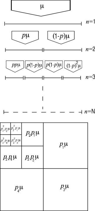
Figure 1: Upper panel: Different steps of generating multifractal rough surface in one Dimension. Lower panel: The same steps for multifractal rough surface in two dimensions [11].

II Multifractal rough surface synthesis

Recently there has been an increasing interest in the notion of multifractality because of its extensive applications in different areas such as complex systems, industrial and natural phenomena. Dozens of methods for the synthesis of multifractal measures or multifractal rough surfaces have been invented. One of the most common methods thath can be followed deterministically and stochastically is the multiplicative cascading process smc ; Feder ; Biolog ; FMTS . Some of these synthesis methods are known as the random $\beta$ model benzi84 , $\alpha$ model scher884 , log-stable models, log-infinitely divisible cascade models scher87 ; scher97 and $p$ model smc . They were successfully applied in the studies related to rain in one dimension, clouds in two dimensions and landscapes in three dimensions as well as many other fields scher87 ; scher89 ; scher97 ; wilson91 .

The $p$ model method was proposed to mimic the kinetic energy dissipation field in fully developed turbulence smc . The so-called $p$ model represents the spatial version of weighted curdling feature and is known as conservative cascade . It is based on Richardson’s picture of energy transfer from cores to fine scales base on splitting eddies in a random way frisch In this model there is no divergency in corresponding moments in contrast to the so-called hyperbolic of $\alpha$ model smc ; frisch1

On the other hand, many scaling exponents of mentioned model can be determined analytically; therefore, it is a proper method to simulate synthetic multifractal processes ranging from surface sciences and astronomy to high energy physics such as cosmology and particle physics e.g QCD parton shower cascades, and cosmic microwave background radiation ochs ; brax ; perivol . In the context of $p$ model simulating a synthetic one-dimensional data set, consider an interval with size $L$. Divide $L$ into two parts with equal lengths. The value of the left half corresponds to the fraction $0\leq p\leq 1$ of a typical measure $\mu$ while the right hand segment is associated to the remaining fraction $(1-p)$. By increasing the resolution to $2^{-n}$, the multiplicative process divides the population in each part in the same way (see the upper panel of Fig. 1).

To simulate a mock multifractal rough surface in two dimensions, one can follow the same procedure as above. Starting from a square, one breaks it into four sub-squares of the same sizes. The associated measures for each cell at this step are $p_{1}\mu$ for the upper right cell, $p_{2}\mu$ for the upper left cell, $p_{3}\mu$ for the lower right cell and $p_{4}\mu$ for the lower left cell. The conservation of probability at each cascade step is $p_{1}+p_{2}+p_{3}+p_{4}=1$. This partitioning and redistribution process repeat and we obtain after many generations, say $n$, $2^{n}\times 2^{n}$ cells of size $l/L=2^{-n}$ (see lower panel of Fig. 1). In the stochastic approach, the fraction of measure for each sub-cell at an arbitrary generation is determined by a random variable ${\mathcal{A}}$ with a definite probability distribution function $P({\mathcal{A}})$. By redistribution of measure, based on independent realization of the random ${\mathcal{A}}$ at smaller scales, one can generate a random singular measure over a substrate with size $L\times L$ as

$$\mu_{n}(\mathbf{r};l)=\mu\prod_{i=1}^{n(l)}{\mathcal{A}_{i}(\mathbf{r})},\quad\quad n(l)=\log_{2}\left(\frac{L}{l}\right)\rightarrow\infty,$$ (1)

where $\mathbf{r}$ shows the coordinate of the underlying cell with size $l$. In this work, we rely on the stochastic version of the cascade $p$ model to generate the synthetic two-dimensional multifractal rough surface (see Figs. 2 and 3). The probability distribution function for our approach is given by

$$P({\mathcal{A}}) = \frac{1}{4}[\delta({\mathcal{A}}-{\mathcal{A}}_{1})+\delta({\mathcal{A}}-{\mathcal{A}}_{2})$$ (2)

$$+\delta({\mathcal{A}}-{\mathcal{A}}_{3})+\delta({\mathcal{A}}-{\mathcal{A}}_{4})],$$

where

$${\mathcal{A}}_{1} = p_{1},\quad{\mathcal{A}}_{2}=p_{2},$$

$${\mathcal{A}}_{3} = p_{3},\quad{\mathcal{A}}_{4}=p_{4}.$$ (3)

The so-called multifractal scaling exponent, $\tau(q)$, and the generalized Hurst exponent, $h(q)$, are quantities that represent the multifractal behaviors of rough surfaces (see section III for more details). For $p$ model cascade, these exponents can be calculated explicitly. The scaling exponent $\tau(q)$ is defined via partition function as

$$Z_{q}(l)=\lim_{l\rightarrow 0}\sum_{i=1}^{n(l)}|P({\mathcal{A}}_{i},l)|^{q}\sim l^{\tau(q)}.$$ (4)

Using the value of $P({\mathcal{A}})$, e.g. for binomial cascade model $P({\mathcal{A}})=\frac{1}{2}[\delta({\mathcal{A}}-p)+\delta({\mathcal{A}}-(1-p)]$, one finds

$$\tau(q) = \lim_{l\rightarrow 0}\frac{\log(Z_{q}(l))}{\log(l)}$$ (5)

$$= (E-1)(q-1)-\log_{2}(p^{q}+(1-p)^{q}),$$

where $E$ is the dimension of the geometric support, where for our rough surfaces is $E=2$. For generalized $p$ model, the analytic expression of multifractal scaling exponent in two dimensions is given by Kadanoff

$$\tau(q)=-\log_{2}(p_{1}^{q}+p_{2}^{q}+p_{3}^{q}+p_{4}^{q}).$$ (6)

One can use the above theoretical expression to get the most relevant quantities of the multifractal behavior and check the reliability and the robustness of numerical method.

Recently, factorial moments, G-moments, correlation integrals, void probabilities, combinants and wavelet correlations have been used to examine many interesting feature of multiplicative cascade processes casc . But there is some ambiguity in properties of such processes that represent multifractal phenomena. On the other hand, sensitivity and accuracy of results are method dependent; consequently, it is highly proposed to simultaneously use various tools in order to ensure the reliability of given results for underlying multifractal rough features. Moreover, to make a relation between experimental data and simulation, generally, we require more than one characterization KHS ; gomez

In the next section, to investigate the multifractal properties of simulated rough surfaces in two dimensions, we will introduce the so-called multifractal detrended fluctuation analysis.

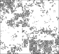
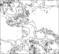
Figure 2: Left: Contour plot at some typical levels of a singular multifractal rough surface generated by binomial cascade multifractal method with $p=0.22$($H=0.803$). The right panel indicates the contour lines of the same surface convolved with $H^{*}=0.700$. The system size is $256\times 256$.

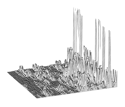
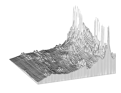
Figure 3: Upper panel: A part of height fluctuations of singular measure mentioned in Fig. 2. Lower panel: The same surface convolved with $H^{*}=0.700$.

III Multifractality of synthesis rough surface

There are many different methods to determine the multiscaling properties of real as well as synthetic multifractal surfaces such as spectral analysis SA1 , fluctuation analysis FA , detrended fluctuation analysis (DFA) DFA1 ; DFA2 ; DFA3 , wavelet transform module maxima (WTMM) wave ; wavelet-based method ; wt1 ; wt2 ; wt3 and discrete wavelets kantelh95 ; kantelh96 . For real data sets and in the presence of noise, the multifractal DFA (MF-DFA) algorithm gives very reliable results Biolog ; DFA2 . Since it does not require the modulus maxima procedure therefore this method is simpler than WTMM, however, it involves a bit more effort in programming.

In this work, we rely on the two dimensional multifractal detrended fluctuation analysis (MF-DFA) to determine the spectrum of the generalized Hurst exponent, $h(q)$. We then compare given results with theoretical prediction to check the reliability of our simulation. Suppose that for a rough surface in two dimensions height of the fluctuations is represented by ${\mathcal{H}}(\mathbf{r})$ at coordinate $\mathbf{r}=(i,j)$ with resolution $\Delta$. The MF-DFA in two dimensions has the following steps Biolog

Step1: Consider a two dimensional array ${\mathcal{H}}(i,j)$ where $i=1,2,...,M$ and $j=1,2,...,N$. Divide the ${\mathcal{H}}(i,j)$ into $M_{s}\times N_{s}$ non-overlapping square segments of equal sizes $s\times s$, where $M_{s}=[\frac{M}{s}]$ and $N_{s}=[\frac{N}{s}]$. Each square segment can be denoted by ${\mathcal{H}}_{\nu,w}$ such that ${\mathcal{H}}_{\nu,w}(i,j)={\mathcal{H}}(l_{1}+i,l_{2}+j)$ for $1\leq i,j\leq s$, where $l_{1}=(\nu-1)s$ and $l_{2}=(w-1)s$.

Step 2: For each non-overlapping segment, the cumulative sum is calculated by:

$$Y_{\nu,w}(i,j)=\sum_{k_{1}=1}^{i}\sum_{k_{2}=1}^{j}{\mathcal{H}}_{\nu,w}(k_{1},k_{2});$$ (7)

where $1\leq i,j\leq s$.

Step 3: Calculating the local trend for each segments by a least-squares of the profile, linear, quadratic or higher order polynomials can be used in the fitting procedure as follows:

$${\mathcal{B}}_{\nu,w}(i,j) = ai+bj+c,$$ (8)

$${\mathcal{B}}_{\nu,w}(i,j) = ai^{2}+bj^{2}+c.$$ (9)

Then determine the variance for each segment as follows:

$${\mathcal{D}}_{\nu,w}(i,j) = Y_{\nu,w}(i,j)-{\mathcal{B}}_{\nu,w}(i,j),$$ (10)

$$F^{2}_{\nu,w}(s) = \frac{1}{s^{2}}\sum_{i=1}^{s}\sum_{j=1}^{s}{\mathcal{D}}^{2}_{\nu,w}(i,j).$$ (11)

A comparison of the results for different orders of DFA allows one to estimate the type of the polynomial trends in the surface data.

Step 4: Averaging over all segments to obtain the $q$’th order fluctuation function

$$F_{q}(s)=\Big{(}\frac{1}{M_{s}\times N_{s}}\sum_{\nu=1}^{M_{s}}\sum_{w=1}^{N_{s}}\left[F^{2}_{\nu,w}(s)\right]^{q/2}\Big{)}^{1/q},$$ (12)

where $F_{q}(s)$ depends on scale $s$ for different values of $q$. It is easy to see that $F_{q}(s)$ increases with increasing $s$. Notice that $F_{q}(s)$ depends on the order $q$. In principle, $q$ can take any real value except zero. For $q=0$ Eq. (12) becomes

$$F_{0}(s)=\exp\Big{(}\frac{1}{2M_{s}\times N_{s}}\sum_{\nu=1}^{M_{s}}\sum_{w=1}^{N_{s}}\ln F^{2}_{\nu,w}(s)\Big{)}.$$ (13)

For $q=2$ the standard DFA in two dimensions will be retrieved.

Step 5: Finally, investigate the scaling behavior of the fluctuation functions by analyzing log-log plots of $F_{q}(s)$ versus $s$ for each value of $q$,

$$F(s)\sim s^{h(q)}.$$ (14)

The Hurst exponent is given by

$$H\equiv h(q=2)-1.$$ (15)

Using standard multifractal formalism DFA2 we have

$$\tau(q)=qh(q)-E.$$ (16)

It has been shown that for very large scales, $N/4<s$, $F_{q}(s)$ becomes statistically unreliable because the number of segments $N_{s}$ for the averaging procedure in step 4 becomes very small Biolog . Thus, scales $N/4<s$ should be excluded from the fitting procedure of determining $h(q)$. On the other hand one should be careful also about systematic deviations from the scaling behavior in Eq. (12) that can occur for the small scales $s<10$.

The singularity spectrum, $f(\alpha)$, of a multifractal rough surface is given by the Legendre transformation of $\tau(q)$ as

$$f(\alpha)=q\alpha-\tau(q),$$ (17)

where $\alpha=\frac{\partial\tau(q)}{\partial q}$. It is well-known that for a multifractal surface, various parts of the feature are characterized by different values of $\alpha$, causing a set of H$\ddot{\rm o}$lder exponents instead of a single $\alpha$. The interval of H$\ddot{\rm o}$lder spectrum, $\alpha\in[\alpha_{\rm min},\alpha_{\rm max}]$, can be determined by muzy94 ; muzy95

$$\alpha_{\rm min} = \lim_{q\rightarrow+\infty}\frac{\partial\tau(q)}{\partial q},$$ (18)

$$\alpha_{\rm max} = \lim_{q\rightarrow-\infty}\frac{\partial\tau(q)}{\partial q}.$$ (19)

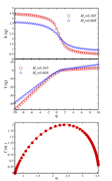
Figure 4: (Color online) Diagrams of $h(q)$ (upper panel) and $\tau(q)$ (middle panel) for different surfaces. We have distinguished different surfaces with their $H_{i}=h_{i}(q=2)-1$ coming from the Table I. The subindex ($i\in[1,12]$) of each $H_{i}$ (Hurst exponent) throughout this paper corresponds to a given set of $p$ values reported in Table I. The lower panel corresponds to the singularity spectrum of a typical multifractal rough surface with $H_{4}=0.608$. In all diagrams, symbols and solid lines correspond to results given by numerical calculation and theoretical formula, respectively.

To evaluate the statistical errors due to numerical calculations we introduce posterior probability distribution function in terms of likelihood analysis. To this end, suppose the measurements and model parameters to be assigned by $\{X\}$ and $\{\Theta\}$, respectively.The conditional probability of the model parameters for a given observation is as follows (posterior)

$$P(\Theta|X)=\frac{{\mathcal{L}}(X|\Theta)P(\Theta)}{\int{\mathcal{L}}(X|\Theta)P(\Theta)d\Theta}.$$ (20)

here ${\mathcal{L}}(X|\Theta)$ and $P(\Theta)$ are called Likelihood and prior distribution, respectively. The prior distribution containing all initial constraints regarding model parameters. Based on the central limit theorem, Likelihood function can be given by a product of gaussian functions as follows:

$$\ln{\mathcal{L}}(X|\Theta)\sim\frac{-\chi^{2}(\Theta)}{2},$$ (21)

where e.g., for determining $h(q)$ we have $\{X\}:\{F_{q}(s)\}$ as observations and $\{\Theta\}:\{h(q)\}$ as free parameter to be determined. Also

$$\chi^{2}(h(q))=\sum_{s}\frac{[F_{{\rm obs.}}(s)-F_{{\rm the.}}(s;h(q))]^{2}}{\sigma_{{\rm obs.}}^{2}(s)},$$ (22)

where $F_{{\rm obs.}}(s)$ is computed by Eqs. (12) and (13). $F_{{\rm the.}}(s;h(q))$ is the fluctuation functions given by Eq. (14). The observational error is $\sigma_{{\rm obs.}}(s)$. By using the fisher matrix, one can evaluate the value of the error-bar at $1\sigma$ confidence interval of $h(q)$ fisher

$$\mathcal{F}(q)\equiv\left\langle\frac{\partial^{2}\ln\mathcal{L}}{\partial h(q)^{2}}\right\rangle$$ (23)

and

$$\sigma(q)\simeq\frac{1}{\sqrt{\mathcal{F}(q)}}$$ (24)

Finally we report the best value of the scaling exponent at $1\sigma$ confidence interval according to $h(q)\pm\sigma(q)$. Using the method mentioned in the previous section, we simulated multifractal rough surfaces and checked their multifractality nature by using the spectrum of $h(q)$. Figure 4 shows the generalized Hurst exponent and $\tau(q)$ as a function of $q$ for various values of measure sets reported in Table 1. The subindex ($i\in[1,12]$) of each $H_{i}$ (Hurst exponent) throughout this paper corresponds to a given set of $p$ values reported in Table 1. In addition the singularity spectrum of a typical simulated multifractal rough surface has been shown in the lower panel of Fig. 4. The $q$ dependence of $h(q)$ as well as the extended range of singularity spectrum demonstrate the multifractality nature of synthesis rough surfaces. Theoretical predictions of $\tau(q)$, $h(q)$ and $f(\alpha)$ shown by the solid lines in the corresponding plots, are given by Eqs. (6), (16) and (17), respectively. There is a good consistency between theoretical predictions and computational values.

Before going further it is worth mentioning that in the cascade $p$ model for various sets of $p$ values which have the same $h(q=2)$, in principle, there exist different $h(q)$ spectrums. To show this point, we fixed the value of $\tau(q=2)$ in Eq. (6) and by having e.g., $p_{1}$ and $p_{2}$, one can compute the rest of $p$ values according to normalization of $p$’s. In Fig. 5 we show MF-DFA results of various sets of $p$ values causing the same so-called $h(q=2)$ exponents. Subsequently, it is expected that for characterizing the geometrical properties of underlying surfaces, one must take into account full spectrum of generalized Hurst exponents.

Hurst exponent	$p_{1}$	$p_{2}$	$p_{3}$	$p_{4}$
$H_{1}=0.305$	$0.040$	$0.800$	$0.080$	$0.080$
$H_{2}=0.404$	$0.100$	$0.740$	$0.080$	$0.080$
$H_{3}=0.504$	$0.120$	$0.680$	$0.110$	$0.090$
$H_{4}=0.608$	$0.190$	$0.610$	$0.130$	$0.070$
$H_{5}=0.608$	$0.090$	$0.100$	$0.610$	$0.200$
$H_{6}=0.608$	$0.600$	$0.100$	$0.237$	$0.063$
$H_{7}=0.608$	$0.350$	$0.100$	$0.546$	$0.004$
$H_{8}=0.706$	$0.210$	$0.550$	$0.130$	$0.110$
$H_{9}=0.802$	$0.220$	$0.480$	$0.200$	$0.100$
$H_{10}=0.697$	$0.120$	$0.180$	$0.560$	$0.140$
$H_{11}=0.806$	$0.160$	$0.180$	$0.170$	$0.490$
$H_{12}=0.906$	$0.410$	$0.200$	$0.210$	$0.180$

Table 1: The $p$ values used for construction of surfaces with various Hurst exponents, $H_{i}=h_{i}(q=2)-1$. The subindex ($i\in[1,12]$) of $H_{i}$ represents the label of different sets of $p$ values.

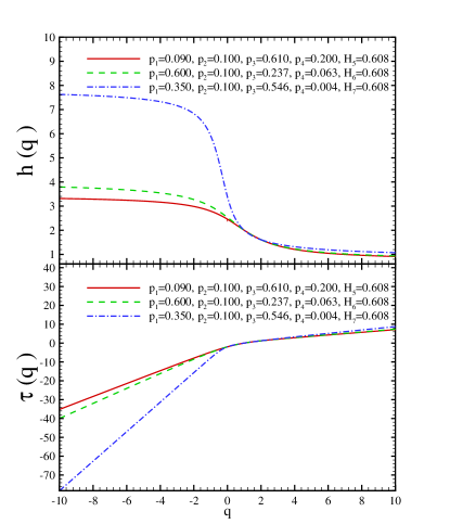
Figure 5: (Color online) The multifractal spectrum of surfaces produced by different sets of $p$ values but with the same $h(q=2)$ up to our numerical precision.

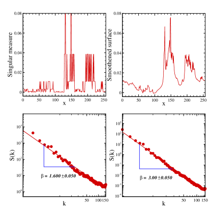
Figure 6: (Color online) Upper panel: Pprofile of singular (left) and smoothened (right) multifractal rough surfaces along a typical horizontal cut in Fig. 2. Lower panel: Spectral density of mentioned mock rough surfaces. The solid lines in the lower panel corresponds to a power law fitting function and symbols are given by numerical calculation. Here we took $H^{*}=0.700$.

It must be pointed out that the generated surfaces have some discontinuities (see Fig. 2). To make them smooth, a proper way is using fractionally integrated singular cascade (FISC) method wavelet-based method . In this method, the multifractal measure is transformed into a smoother multifractal rough surface by filtering the singular multifractal measure [$\mu(\mathbf{r})$, (Eq. (1))] in the Fourier space as

$${\mathcal{H}}(\mathbf{r})=\mu(\mathbf{r})\otimes|\mathbf{r}|^{-(1-H^{*})},$$ (25)

where $\otimes$ is the convolution operator and $H^{*}\in(0,1)$ is the order of smoothness (see the right panel of Fig. 2 and lower panel of Fig. 3). In this case $\tau_{f}(q)$ reads as

$$\tau_{f}(q)=\tau(q)+qH^{*},$$ (26)

where $\tau(q)$ is given by Eq.(6). Using the correlation function, $C(|\mathbf{r}|)\sim|\mathbf{r}|^{-\gamma}$, and its Fourier transform one can derive the power spectrum scaling exponent $\beta$ of the singular as well as the smoothened synthetic multifractal surfaces. To this end we demand the scaling behavior for power spectrum to be

$$S(k)\sim|\mathbf{k}|^{-\beta},$$ (27)

where $\mathbf{k}=(k_{x},k_{y})$, $k_{x}=\frac{2\pi}{\Delta\times N}i$, $k_{y}=\frac{2\pi}{\Delta\times N}j$ and $(i,j)$ run from $1$ to $N=L/\Delta$ (the pixel of system size). Subsequently the power spectrum scaling exponent is given by wavelet-based method

$$\beta = 1+2H^{*}-\log_{2}(p^{2}+(1-p)^{2}).$$ (28)

To make more sense, in Table 2 we collected the correlation and power spectrum exponents of stochastic processes in one and two dimensions .

Exponent	1D-fGn	1D-fBm	2D-Cascade	2D-fBm
$\gamma$	$2-2H$	$-2H$	$1-2H$	$-1-2H$
$\beta$	$2H-1$	$2H+1$	$2H$	$2H+2$

Table 2: The most relevant exponents concerning stochastic processes in one and two dimensions.

Figure 6 indicates one dimension profiles obtained along a typical horizontal cut in Fig. 2 for singular and smoothened multifractal rough surfaces. The lower panels of Fig. 6 show the power spectrums of simulated rough surfaces. The convolution does not change the multifractality nature of singular measure (see Fig. 7). In this plot one can see that the synthetic smoothened surface remains multifractal.

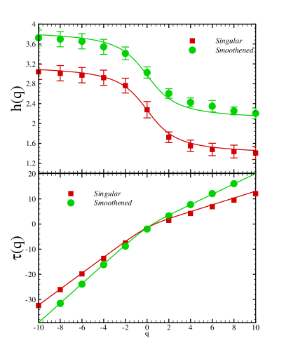
Figure 7: (Color online) Generalized Hurst exponent of singular measure for $H_{9}=0.802$ (square symbols) and that of convolved with $H^{*}=0.700$ (circle symbols). The solid lines are from the theory.

IV Geometrical exponents of contour loops

For a given multifractal rough surface with the height ${\mathcal{H}}(\mathbf{x})$, a level set ${\mathcal{H}}(\mathbf{x})={\mathcal{H}}_{0}$ for different values of ${\mathcal{H}}_{0}$ consists of many closed non-intersecting loops. These loops are recognized as contour loops. The contour loop ensemble corresponds to contour loops of various level sets. In Fig. 2 we plotted a set of contour loop at some typical levels for singular multifractal rough surface and corresponding convolved surface with $H^{*}=0.700$. The loop length $s$ can be defined as the total number of unit cells constructing a contour loop multiplied by lattice constant $\Delta$. The radius of a typical loop is represented by $R$ and it is the side of the smallest box that completely enwraps the loop. For a mono-fractal surface, these loops are usually fractal and their size distribution is characterized by a few scaling functions and scaling exponents. For example the contour line properties can be described by the loop correlation function $G(\mathbf{r})$. The loop correlation function measures the probability that the two points separated by the distance $\mathbf{r}$ in the plane lie on the same contour. Rotational invariance of the contour lines forces $G(\mathbf{r})$ to depend only on $r=|\mathbf{r}|$. This function for the contours on the lattice with grid size $\Delta$ and in the limit $r\gg\Delta$ has the scaling behavior

$$G(r)\sim r^{-2x_{l}},$$ (29)

where $x_{l}$ is the loop correlation exponent. It was shown numerically KH ; KHS ; Ghasemi_Rajabpour that for all the known mono-fractal rough surfaces this exponent is superuniversal and equal to $\frac{1}{2}$. A key consequence of this result is that, the contour loops with perimeter $s$ and radius $R$ of such surfaces are self-similar. When these lines are scale invariant, one can determine the fractal dimension as the exponent in the perimeter-radius relation. The relation between contour length $s$ and its radius of gyration $R$ is

$$\langle s\rangle(R)\sim R^{D_{f}},$$ (30)

where $D_{f}$ is the fractal dimension and $R$ is defined by $R^{2}=\frac{1}{N}\sum_{i=1}^{N}\Big{[}(x_{i}-x_{c})^{2}+(y_{i}-y_{c})^{2}\Big{]}$, with $x_{c}=\frac{1}{N}\sum_{i=1}^{N}x_{i}$ and $y_{c}=\frac{1}{N}\sum_{i=1}^{N}y_{i}$ being the central mass coordinates. The $D_{f}$ is the fractal dimension of one contour and for mono fractal rough surfaces is given by $D_{f}=\frac{3-H}{2}$ KHS . Depending on what feature of the multifractal rough surface is under investigation one can get various types of fractal dimensions. In this paper we introduce the fractal dimension of a isoheight line, $D_{f}$, and the fractal dimension of all the level set, $d$. The generalized form of fractal dimension can be expressed by means of partition function of underlaying feature, which is contours in this context, as

$$D(q)=\lim_{l\rightarrow 0}\frac{1}{q-1}\frac{\log(Z_{q}(l))}{\log(l)},$$ (31)

where $l$ is the size of the cells that one uses to cover the domain and its minimum value is equal to grid size, $\Delta$. $Z_{q}(l)$ is the partition function defined in Eq. (4) but here it should be constructed by using contour loops instead of height function and $q$ can be any real number. It is easy to show that $D(q=0)=D_{f}$ and $D(q=1)$ corresponds to the so-called entropy of underlying system Kadanoff .

For a given self-similar loop ensemble, one can define the probability distribution of contour lengths $\tilde{P}(s)$. This function is a measure for the total loops with length $s$ and follows the power law

$$\tilde{P}(s)\sim s^{-\eta},$$ (32)

where $\eta$ is a scaling exponent. Another interesting quantity with the scaling property is the cumulative distribution of the number of contours with area greater than $A$ which has the following form

$$P_{>}(A)\sim A^{-\frac{\xi}{2}}.$$ (33)

For mono fractal rough surfaces we have $\xi=2-H$. Using the scaling property of the mono-fractal surfaces it was shown that the three exponents $D_{f}$, $\eta$, $\xi$ and $x_{l}$ satisfy the following hyperscaling relations KH

$$D_{f}=\frac{\xi}{(\eta-1)},$$ (34)

$$D_{f}=\frac{2x_{l}-2}{\eta-3}.$$ (35)

Using the above relations it is easy to get the relation between $\eta$ and Hurst exponent $H$. Before closing this section, we summarize all of the exponents introduced in this section in Table 3.

Exponent	Relation	Description
$x_{l}$	$G(r)\sim r^{-2x_{l}}$	Loop correlation exponent
$D_{f}$	$\langle s\rangle(R)\sim R^{D_{f}}$	Fractal dimension of a contour loop
$D(q)$	Eq. (31)	Multifractal dimension
$d$	$N(l)\sim l^{-d}$	Fractal dimension of all contour set
$\eta$	$\tilde{P}(s)\sim s^{-\eta}$	Length distribution exponent
$\xi$	$P_{>}(A)\sim A^{-\frac{\xi}{2}}$	Area cumulative exponent

Table 3: The relevant exponents introduced in this paper to characterize synthetic multifractal rough surfaces.

In the next section we will calculate all mentioned exponents by using different numerical methods for singular as well as smoothened multifractal rough surfaces and we will examine the validity of the hyperscaling relations in this context.

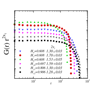
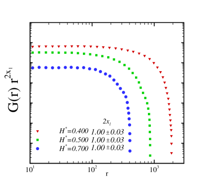
Figure 8: (Color online) Log-log diagram of $r^{2x_{l}}G(r)$ versus $r$ for different Hurst exponents. Upper panel corresponds to singular measure with the sets of $p$ values reported in Table I. Lower panel is indicates loop correlation function for smoothened multifractal surface for various $H^{*}$’s. In these figures we shifted the $y$ axis vertically.The system size is $4096\times 4096$.

V Numerical results

In order to examine the geometrical exponents of the contour loops mentioned in Table 3 of synthetic multifractal rough surfaces, we have generated multifractal rough surfaces with different $h(q=2)$’s using the typical measures reported in Table 1. We have generated $100$ ensembles of each surfaces with various sizes ranging from $(2048\times 2048)$ to $(4096\times 4096)$. To extract the contour loops of the mock multifractal rough surfaces at mean height, ${\mathcal{H}}_{0}$, we use two different methods, the contouring algorithm and Hoshen-Kopelman algorithm Vaez_Rajabpour . According to our results, these two methods give almost the same results for geometrical exponents. In the next subsections we present our numerical results concerning the exponents introduced in the preceding sections.

V.1 Loop correlation function exponent

The loop correlation function exponent $x_{l}$ is the most central exponent in mono-fractal rough surfaces. It is independent of $H$ and is equal to $\frac{1}{2}$. This result has also been proven for $H=0$ according to the exact solvable statistical mechanics model for contours equivalent to the critical $O(2)$ loop model on the honeycomb lattice nien87 ; KHS .

To find the correlation function from a given loop ensemble for multifractal rough surfaces, we followed the algorithm described in Ref. KHS . We calculated the loop correlation function $G(r)$ for our multifractal rough surfaces (with system size $2048\times 2048$ and averaging is done over $10$ realizations). The log-log diagram of $G(r)r^{2x_{l}}$ versus $r$ for different sets of $p$ values ($H_{i}=h_{i}(q=2)-1$ for some $i\in[1,12]$) have been shown in the Fig. 8. Each set corresponds to a synthetic multifractal rough surface generated according to the algorithm presented in section II. Our results demonstrate that the $x_{l}$ exponent, not only depends on the value of the Hurst exponent but also depend on the different sets of $p$ values (see the upper panel of Fig. 8 ). In other words, as reported in Table 1 as well as shown in upper panel of Fig. (8), the sets $i=4$, $i=5$ and $i=6$ of $p$ values have equal Hurst exponent, nevertheless, the corresponding correlation exponents, $x_{l}$, for these sets differ completely. On the other hand, at the level of our numerical accuracy, as shown in the lower panel of Fig. 8, the value for the smoothened multifractal surfaces correlation exponents is the same as that reported for the mono fractal rough surfaces, namely $x_{l}=\frac{1}{2}$.

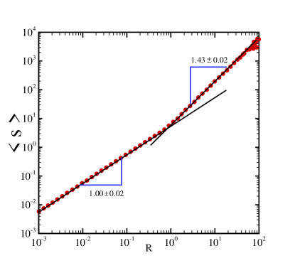
Figure 9: (Color online) The log-log plot of $\langle s\rangle(R)$ versus $R$ for synthetic multifractal singular rough surface for $H_{4}=0.608$.

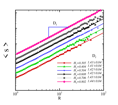
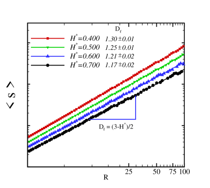
Figure 10: (Color online) Upper panel: Log-log of $\langle s\rangle(R)$ versus $R$ for singular multifractal rough surfaces for various sets of $p$ values reported in Table I. Lower panel: The same diagram for smoothened synthetic multifractal rough surfaces. The sample size is $4096\times 4096$ and the ensemble average was done over $100$ realizations. To make more sense, we shifted the values of $\langle s\rangle$ vertically for different multifractal rough surfaces.

V.2 Fractal dimension

To calculate the fractal dimension of a contour loop, we have calculated the perimeter and radius of gyrations of different contour loops. Figure 9 shows log-log plot of $\langle s\rangle(R)$ versus $\langle R\rangle$ values for synthetic multifractal rough surfaces with typical value of Hurst exponent, $H_{4}=0.608$. There are two distinct regions with different slopes in the diagram; the first region is related to a large number of small loops with radius smaller than one $(R<1)$ with $D_{f}=1.00\pm 0.01$. This is not a relevant phenomenon and it comes from the contouring algorithm that produces lots of contour loops around very small clusters (made usually from one cell). In the second region $(R>1)$ the slope increases to $1.43\pm 0.02$ and it keeps to follow the scaling behavior up to very large sizes. The slopes for different Hurst exponent follow the relation $D_{f}=(3-H)/2$ for mono-fractal case KHS . For various values of the Hurst exponent our computation is shown in the upper panel of Fig. 10 (see also Table 4). At $1\sigma$ confidence interval all slopes are the same. On the contrary, in the case of the contour lines of the convolved rough surfaces with arbitrary $H^{*}$’s the fractal dimension of a contour line follows the formula of a mono fractal surface with $H=H^{*}$, namely $D_{f}=(3-H^{*})/2$. It is quite interesting that these results are completely independent form the $p$ values (lower panel of Fig. 10). This simply means that the fractal dimension of the contour loops of the singular rough surfaces does not change with respect to the $h(q=2)$. In other words, in contrast to the mono fractal case, $h(q=2)$ alone can not represent the properties of the underlying singular multifractal rough surface.

We also calculated the fractal dimension by using partition function introduced in Eqs. (4) and (31). Figure 11 shows $D(q)$ as a function of $q$. The $q$ dependance of these results confirms that contour loops of synthetic singular and smooth multifractal rough surfaces are multifractal. For $q=0$ at $68\%$ confidence interval $D(q=0)=1.46\pm 0.05$. This is also in agreement with the value determined by calculating the scaling behavior of the contour sizes. In addition as we may expect this diagram demonstrates that the isoheight contour loops of underlying simulated multifractal rough surfaces behave as a multifractal feature .

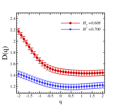
Figure 11: (Color online) Generalized fractal dimension versus $q$ for singular measure with $H_{4}=0.608$ and that of convolved by $H^{*}=0.700$. For singular and smoothened surfaces $D_{f}=1.46\pm 0.05$ and $D_{f}=1.19\pm 0.05$, respectively.

As mentioned , the fractal dimension of all the contours, $d$, differs from the fractal dimension of a contour loop $D_{f}$. The fractal dimension of a contour set for mono fractal rough surfaces is given by $d=2-H$. For the smoothened multifractal rough surfaces introduced by Eq. (25), the fractal dimension of the contour set is $d=2-H^{*}$ wt1 . We have calculated the fractal dimension of the contour set by using the box counting method. As previously, we used a least-squares equation (Eq. (21)) to determine the slope in the log-log diagram of the number of segments that will cover the underlying feature $N(l)$ versus length scale $l$ for different Hurst exponents. To obtain best fit value for the slope corresponding to our data, as well as its error, we divided the data into different ranges and determined the slope by least-squares method. To do so according to likelihood function (Eq. (21)), we define $\chi^{2}$ as

$$\chi^{2}(d)=\sum_{i=1}^{\mathcal{N}}\frac{[N(l_{i})-N_{\rm the.}(l_{i};d)]^{2}}{\sigma(l_{i})^{2}},$$ (36)

where ${\mathcal{N}}$ is the number of partitioning, namely ${\mathcal{N}}=L/l_{\mathcal{N}}$, $N_{\rm the.}(l_{i};d)\sim l_{i}^{-d}$ and $\sigma^{2}(l_{i})$ is the variance of the data in the corresponding range. Finally we determined the minimum $\chi^{2}$ and the best slope for the data. Figure 12 corresponds to synthetic smoothened multifractal rough surfaces. In addition we checked that whether the result associated to the smoothened rough surfaces depends on the set of $p$ values correspond to the same value of $h(q=2)$. Our findings confirm that $d$ doesn’t depend on different sets of $p$ values. However, for the singular measure, $d$ depends on the value of $H$ and even $p$’s used for the cascade algorithm. It has no regular behavior with respect to $h(q=2)$. Moreover for various sets of $p$ values giving the same value of $h(q=2)$, one finds out different values for fractal dimension of all contour sets. This is quite surprising because for singular measure multifractal surface, we have $H^{*}=0$ and, therefore, if the formula $2-H^{*}$ was correct in this regime, we should have $d=2$ for all the different $h(q=2)$’s. We are not aware of any theoretical argument that can explain this phenomenon.

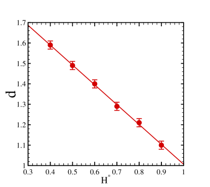
Figure 12: (Color online) Fractal dimension of all contours of the smoothened multifractal surfaces as a function of $H^{*}$. The solid line corresponds to linear fitting function.

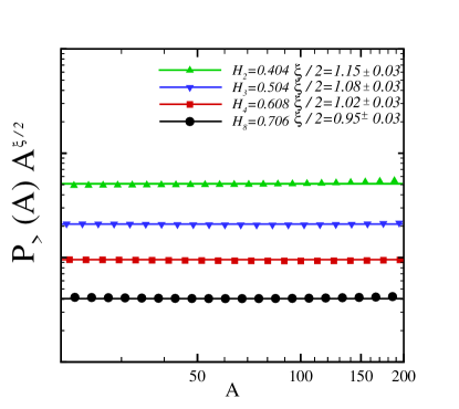
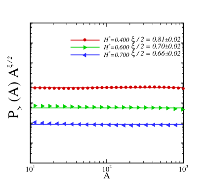
Figure 13: (Color online) Upper panel: The cumulative distributions of the areas of the contour loops with respect to the area for the singular multifractal rough surfaces. The corresponding set of $p$ values is given in Table I. Lower panel: The same distribution for the smoothened multifractal surfaces. For clarity, we shifted the value of $y$ axis vertically for both diagrams.

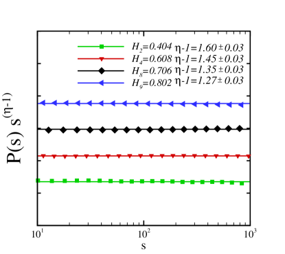
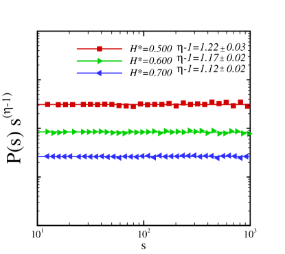
Figure 14: (Color online) Upper panel:The perimeter distribution exponent for different sets of $p$ values of the singular measure. Lower panel the same measure for the smoothened multifractal rough surfaces. The values of $y$ axis are shifted vertically.

V.3 Cumulative distribution of areas

To calculate the exponent $\xi$ we have calculated the $P_{>}(A)A^{\xi/2}$ with respect to the area of the contour loops. In Fig. 13 and table 4 we have shown the results for various values of Hurst exponent reported in table 1 and averaging is done over 100 realizations. The results are quite different from what we expect for mono-fractal rough surfaces. For mono fractal rough surfaces we have $\xi=2-H$. It must be pointed out that for synthetic singular multifractal rough surfaces $\xi$ decreases by increasing $H$, which is the same as mono-fractal rough surfaces. In addition $\xi$ not only depends on $h(q=2)$ but also is affected by other values of $h(q)$’s. This finding is due to the multifractality nature of the singular measure rough surface. The same computation for the smoothened multifractal rough surfaces is shown in lower panel of Fig. 13. This results confirm that the exponent is controlled by $H^{*}$, and $\xi$ is given by the same equation as for the mono fractal rough surfaces.

V.4 Probability distribution of contour length

Final remark concerns the probability distribution of contour length. To this end we investigated the logarithmic diagram of $P(s)s^{\eta-1}$ versus $s$. We have depicted the results for the synthetic singular as well as smoothened multifractal surfaces for various values of $h(q=2)$. For the smoothened multifractal rough surfaces again the exponents follow the behavior of the mono fractal surfaces (see Fig. 14).

In spite of the huge difference between the geometrical exponents of the contour loops of mono-fractal rough surfaces and singular multifractal rough surfaces, the hyperscaling relations $\frac{\xi}{D_{f}}=\eta-1$ and $D_{f}=\frac{2x_{l}-2}{\eta-3}$ are valid up to numerical accuracy (see Table. 4 and Table. 5). The important factors in obtaining this hyperscaling relation concern power-law relations for $\tilde{P}(s)$ and $P_{>}(A)$. The second hyperscaling relation comes from the following equality

$$\int_{0}^{R}G(r)d^{2}r\sim\int_{0}^{\infty}\min(s,R^{D_{f}})P(s)ds.$$ (37)

Both sides are proportional to the mean of the length of that portion of the contours passing through origin which lies within a radius $R$ from the origin KH .

$H$	$\eta$	$D_{f}$	$\xi$	$2x_{l}$
$H_{1}=0.305$	$2.67\pm 0.03$	$1.43\pm 0.04$	$2.44\pm 0.06$	$1.60\pm 0.10$
$H_{2}=0.404$	$2.60\pm 0.03$	$1.41\pm 0.04$	$2.30\pm 0.06$	$1.49\pm 0.10$
$H_{3}=0.504$	$2.50\pm 0.03$	$1.42\pm 0.04$	$2.16\pm 0.06$	$1.25\pm 0.05$
$H_{4}=0.608$	$2.45\pm 0.02$	$1.42\pm 0.04$	$2.04\pm 0.06$	$1.30\pm 0.03$
$H_{5}=0.608$	$2.74\pm 0.02$	$1.43\pm 0.04$	$2.50\pm 0.06$	$1.70\pm 0.03$
$H_{6}=0.608$	$2.64\pm 0.02$	$1.42\pm 0.04$	$2.31\pm 0.06$	$1.53\pm 0.03$
$H_{8}=0.706$	$2.35\pm 0.02$	$1.43\pm 0.04$	$1.90\pm 0.06$	$1.12\pm 0.03$
$H_{9}=0.802$	$2.27\pm 0.02$	$1.44\pm 0.04$	$1.80\pm 0.06$	$1.02\pm 0.03$

Table 4: Different geometrical exponents of the contour loops extracted from surfaces with different sets of $p-$values reported in Table I. Theses values completely dependent on the $p$ values.

$H$	$\eta-1$	$\frac{\xi}{D_{f}}$	$3D_{f}+2x_{l}$	$D_{f}\eta+2$
$H_{1}=0.305$	$1.67\pm 0.03$	$1.71\pm 0.06$	$5.89\pm 0.16$	$5.82\pm 0.12$
$H_{2}=0.404$	$1.60\pm 0.03$	$1.63\pm 0.06$	$5.72\pm 0.16$	$5.67\pm 0.12$
$H_{3}=0.504$	$1.50\pm 0.03$	$1.52\pm 0.06$	$5.51\pm 0.13$	$5.55\pm 0.11$
$H_{4}=0.608$	$1.45\pm 0.02$	$1.44\pm 0.06$	$5.56\pm 0.12$	$5.48\pm 0.10$
$H_{5}=0.608$	$1.74\pm 0.02$	$1.75\pm 0.06$	$5.99\pm 0.12$	$5.92\pm 0.11$
$H_{6}=0.608$	$1.64\pm 0.02$	$1.63\pm 0.06$	$5.79\pm 0.12$	$5.75\pm 0.11$
$H_{8}=0.706$	$1.35\pm 0.02$	$1.33\pm 0.06$	$5.41\pm 0.12$	$5.36\pm 0.10$
$H_{9}=0.802$	$1.27\pm 0.02$	$1.25\pm 0.05$	$5.34\pm 0.12$	$5.27\pm 0.10$

Table 5: Verification of two basic hyperscaling relations for synthetic singular measure multifractal rough surfaces.

Exponent	Singular measure	Smoothened multifractal
$x_{l}$	Depends on $p-$values	$\frac{1}{2}$
$D_{f}$	Identical	$\frac{3-H^{*}}{2}$
$D(q)$	Depends on $q$	Depends on $q$
$d$	Depends on $p-$values	$2-H^{*}$
$\eta-1$	Depends on $p-$values	$\frac{4-2H^{*}}{3-H^{*}}$
$\xi$	Depends on $p-$values	$2-H^{*}$
$\frac{\xi}{D_{f}}=\eta-1$	YES	YES
$D_{f}=\frac{2x_{l}-2}{\eta-3}$	YES	YES

Table 6: A summarization of results given in this paper based on contouring analysis for synthetic singular and smoothened multifractal rough surfaces.

VI Conclusion

In this paper we have studied the contour lines of particular multifractal rough surfaces, namely the so-called multiplicative hierarchical cascade $p$ model. Utilizing a stochastic cascade method Feder ; Biolog , singular measure (original) and smoothened (convolved) multifractal rough surfaces with different Hurst exponents were generated. The $h(q)$ spectrums of these two dimensional surfaces were determined by MF-DFA method Biolog . Then use of two different algorithms we generated the contour loops of the systems. Many different geometrical exponents, such as the fractal dimension of a contour loop, $D_{f}$ the fractal dimension of the contour set, $d$, the cumulative distributions of perimeters and areas and the correlation exponents, $x_{l}$, were calculated for the singular and smoothened multifractal surfaces by use of different methods.
We summarize the most important results given in this study as follows. Our results confirmed that, the exponent of loop correlation function, $x_{l}$, for multifractal singular measure, depends on $p$ values. On the contrary, for multifractal smoothened surfaces, this value behaves the same as that of given for mono fractal rough surfaces (see Fig. 8).
The scaling exponent of the size of the contours as a function of the radius representing fractal dimension, $D_{f}$, is similar for various singular multifractal rough surfaces. But the relation between $D_{f}$ and $H^{*}$ for convolved multifractal surfaces is similar to mono fractal surfaces. Nevertheless the contour loops have multifractal nature (see Figs. 10 and 11).
The exponent of cumulative distribution of areas, $\xi$, for singular measure has multifractal nature. But for smoothened surface, this quantity is controlled by $H^{*}$ according to $\xi=2-H^{*}$ and is completely independent of $p$ values (see Fig. 13).
Consequently, in the case of singular measure surfaces, all of the exponents show significant deviations from the well-known formulas for the mono-fractal rough surfaces. They depend on the generalized Hurst exponents $h(q)$, whreas for convolved multifractal surfaces, all geometrical exponents are controlled by $H^{*}$ according to a mono fractal system. We emphasize that interestingly, the hyperscaling relations, namely, $\frac{\xi}{D_{f}}=\eta-1$ and $D_{f}=\frac{2x_{l}-2}{\eta-3}$ at $1\sigma$ confidence interval, are valid for both singular and smoothened multifractal rough surfaces(see Table. 4, 5). In this system which is labeled by $H^{*}$, many relevant properties are controlled by a few relations that have been presented for mono-fractal cases. However singular and smoothened multifractal surfaces have multifractal nature but using geometrical analysis, they belong to different class which is a non-trivial result. Table 6 contains most important results given in this paper.

Finally, to make more complete this study, it is useful to extend this approach for various simulated rough surfaces by use of different methods and examine their hyperscaling relations. In addition, there are some methods to distinguish various multiplicative cascade methods such as $n$-point statistics martin98 .

Acknowledgments:

We are grateful to M. Ghaseminezhad for cross checking some of the results and also for fruitful discussions. MSM and SMVA are grateful to associate office of ICTP and their hospitality. The work of SMVA was supported in part by the Research Council of the University of Tehran.

References

- (1) D. Sornette, Critical Phenomena in Natural Sciences: Chaos, Fractals, Selforganization and Disorder: Concepts and Tools, Heidelberg, Germany: Springer-Verlag, (2000).
- (2) H. E. Stanley and P. Meakin, Nature 335, 405-409 (1988).
- (3) M. Ausloos and D.H. Berman, Proc. R. Soc. London A 400 , 331(1985).
- (4) J. Feder, Fractals , (Plenum Press New York and London, 1988).
- (5) Plamen Ch. Ivanov, Luis A. Nunes Amaral, Ary L. Goldberger, Shlomo Havlin, Michael G. Rosenblum, Zbigniew R. Struzik and H. Eugene Stanley, Nature 399, 461 (1999).
- (6) C.-K. Peng, S. V. Buldyrev, S. Havlin, M. Simons, H. E. Stanley and A. L. Goldberger, Phys. Rev. E 49, 1685 (1994)
- (7) Armin Bunde, Jurgen Kropp, Hans-Joachim Schellnhuber, The science of disasters: climate disruptions, heart attacks, and market crashes, Vol. 2, (Springer, 2002); Armin Bunde, Shlomo Havlin, Fractals in science, (Springer-Verlag, 1994); S. Hosseinabadi , A. A. Masoudi, and M. S. Movahed, Physica B 405, 2072 (2010); Ajay Chaudhari, Gulam Rabbani and Shyi-Long Lee, Journal of the Chinese Chemical Society, 54(5), 1201 (2007); Ajay Chaudhari, Ching-Cher Sanders Yan and Shyi-Long Lee, Applied Surface Science 238, 513 (2004); M. Vahabi, G. R. Jafari, N. Mansour, R. Karimzadeh and J. Zamiranvari, Journal of Statistical Mechanics: Theory and Experiment (JSTAT), P03002 (2008); Xia Sun, Zhuxi Fu, Ziqin Wu, Physica A 311, 327 (2002);
- (8) Pradipta Kumar Mandal and Debnarayan Jana, Phys. Rev. E 77, 061604(2008).
- (9) A. Arneodo, N. Decoster, P. Kestener et S.G. Roux, Advances In Imaging And Electron Physics 126, 1 (2003).
- (10) S.G. Roux, A. Arneodo et N. Decoster, Eur. Phys. J. B 15, 765 (2000); N. Decoster, S.G. Roux et A. Arneodo, ibid. 15, 739 (2000); A. Arnedo, N. Decoster et S.G. Roux, ibid. B 15, 567 (2000).
- (11) C. Meneveau and K. R. Sreenivasan, Phys. Rev. Lett. 59, 1424 (1987); C. Meneveau and K. R. Sreenivasan, J. Fluid Mech. 224, 429 ( 1991); K. R. Sreenivasan and R. A. Antonia, Annu. Rev. Fluid Mech. 29, 435 (1997).
- (12) R Benzi, G Paladin, G Parisi and A Vulpiani, J. Phys. A: Math. Gen. 17, 3521 (1984).
- (13) J. F. Muzy, E. Bacry, and A. Arneodo, Phys. Rev. Lett. 67, 3515 (1991).
- (14) T. Vicsek, Physica A 168, 490(1990).
- (15) E. Ben-Jacob, O. Shochet, A. Tenenbaum, I. Cohen, A. Czirok and T. Vicsek, Fractals 2, 15 (1994).
- (16) S. Lovejoy, Science 216, 185 (1982); R. F. Cahalan, in Advances in Remote Sensing and Retrieval Methods, edited by A. Deepak, H. Fleming, J. Theon (Deepak Publishing, Hampton, 1989), p. 371
- (17) M. S. Movahed, F. Ghasemi, S. Rahvar, M. R. Tabar, Phys Rev. E 84, 021103 (2011).
- (18) A. I. Zad, G. Kavei, M. R. R. Tabar, and S. M. V. Allaei, J. Phys: Condens. Matter 15, 1889 (2003).
- (19) J. D. Farmer, E. Ott and J.A. Yorke, Physica D 7, 153(1983) ; Peter Grassberger and Itamar Procaccia, Phys. Rev. Lett. 50, 346 (1983). R. Badii and A. Politi, Phys. Rev. Lett. 52, 1661 (1984).
- (20) M. Chekini, M. R. Mohammadizadeh, and S. M. V. Allaei, App. Surf. Sci. 257, 7179 (2011).
- (21) M. S. Movahed, and E. Hermanis, Phys. A 387, 915 (2008).
- (22) J. W. Kantelhardt, arXiv:0804.0747.
- (23) B. Dubuc, J. F. Quiniou, C. Roques-Carmes, C. Tricot, S.W. Zucker, Phys. Rev. A 39, 1500 (1989); T. Higuchi, Physica D 46, 254 (1990); N. P. Greis, H. S. Greenside, Phys. Rev. A 44, 2324 (1991); W. Li, Int. J. of Bifurcation and Chaos 1, 583 (1991); B. Lea-Cox, J.S.Y. Wang, Fractals 1, 87 (1993).
- (24) A. A. Saberi, M. A. Rajabpour, S. Rouhani, Phys. Rev. Lett. 100, 044504, (2008).
- (25) A. A. Saberi, M. D. Niry, S. M. Fazeli, M. R. Rahimi Tabar, and S. Rouhani, Phys. Rev. E 77, 051607 (2008).
- (26) M. A. Rajabpour and S. M. Vaez Allaei, Phys. Rev. E 80, 011115, (2009).
- (27) M. G. Nezhadhaghighi and M. A. Rajabpour, Phys. Rev. E 83, 021122 (2011).
- (28) A. A. Saberi, H. Dashti-Naserabadi, and S. Rouhani, Phys. Rev. E 82, 020101 (2010).
- (29) A. A. Saberi, Appl. Phys. Lett. 97, 154102 (2010).
- (30) J. Kondev, C. L. Henley, Phys. Rev. Lett. 74 (23), 4580, (1995).
- (31) J. Kondev, C. L. Henley and D. G. Salinas, Phys. Rev. E 61 (1), 104, (2000).
- (32) C. Zeng, J. Kondev, D. McNamara, and A. A. Middleton, Phys. Rev. Lett. 80, 109, (1998).
- (33) Ajay Chaudhari, Ching-Cher Sanders Yan and Shyi-Long Lee, J. Phys. A : Math and Gen., 36, 3757 (2003).
- (34) Gao-Feng Gu and Wei-Xing Zhou, Phys. Rev. E 74 , 061104, (2006).
- (35) D. Schertzer and S. Lovejoy, In Turbulent and Chaotic phenomena in fluids, edited by T. Tatsumi, (North-Holland, New-york, 1984), pp. 505-508.
- (36) D. Schertzer, S. Lovejoy, J. Geophys. Res. 92, 9693 (1987).
- (37) D. Schertzer, S. Lovejoy, F. Schmitt, Y. Ghigirinskaya, and D. Marsan, Fractals 5, 427 (1997).
- (38) D. Schertzer, S. Lovejoy, Fractals: Physical Origin and Consequences, edited by L. Pietronero (Plenum, New York, 1989), p. 49.
- (39) J. Wilson, D. Schertzer, S. Lovejoy, Fractals and Nonlinear Variability in Geophysics, edited by D. Schertzer, S. Lovejoy (Kluwer, Dordrecht, 1991), p. 185.
- (40) U. Frisch, Turbulence, Cambridge University Press, Cambridge (1995).
- (41) U. Frisch, P. L. Salem, and M. Nelkin, J. Fluid Mech. 87, 719 (1978).
- (42) W. Ochs and J. Wosiek, Phys. Lett. B 289, 159 (1992); 305, 144 (1993)
- (43) Ph. Brax, J.L. Meunier and R.Peschanski, Z. Phys. C 62, 649 (1994).
- (44) Leandros Perivolaropoulos, Phys. Rev. D 48, 1530 (1993).
- (45) Thomas C. Halsey, Mogens H. Jensen, Leo P. Kadanoff, Itamar Procaccia, and Boris I. Shraiman, Phys. Rev. A 33, 1141 (1986).
- (46) Martin Greiner, Peter Lipa and Peter Carruthers, Phys. Rev. E 51 , 1948 (1995); A. Bialas and R. Peschanski, Nucl. Phys. B 273, 703 (1986);308, 857 (1988); C. B. Chiu and R. C. Hwa, Phys. Rev. D 43, 100(1991); S. Hegyi, Phys. Lett. B 309 443 (1993); H. C. Eggers, P. Lipa, P. Carruthers and B. Buschbeck, Phys. Rev. D 48, 2040 (1993).
- (47) J. M. Gmez-Rodrguez, A. M. Bar and R. C. Salvarezza, J. Vac. Sci. Technol. B 9, 495 (1991).
- (48) H. E. Hurst, Trans. Am. Soc. Civ. Eng. 116, 770, (1951).
- (49) C. K. Peng, S. Buldyrev, A. Goldberger, S. Havlin, F. Sciortino, M. Simons and H. E. Stanley, Nature 356, 168 (1992)
- (50) J. W. Kantelhardt, S. A. Zschiegner, E. Koscielny-Bunde, S. Havlin, A. Bunde, H. E. Stanley, Physica A 316, 87 (2002).
- (51) Kun Hu, Plamen Ch. Ivanov, Zhi Chen, Pedro Carpena and H. E. Stanley Phys. Rev. E 64, 011114 (2001).
- (52) Zbigniew R. Struzik, Arno P. J. M. Siebes, Physica A 309, 388, (2002).
- (53) J. Arrault, A. Arneodo, A. Davis and A. Marshak, Phys. Rev. Lett., 79, 75 (1997).
- (54) J. W. Kantelhardt, H. E. Roman and M. Greiner, Physica A 220, 219 (1995).
- (55) H. E. Roman, J. W. Kantelhardt and M. Greiner, Europhys. Lett. 35, 641 (1996).
- (56) J.F. Muzy, E. Bacry and A. Arneodo, Int. J. of Bifurcation and Chaos 4, 245 (1994).
- (57) A. Arneodo, E. Bacry and J.F. Muzy, Physica A 213, 232 (1994).
- (58) B. A. Bassett, Y. Fantaye, R. Hlozek, J. Kotze, arXiv:0906.0993.
- (59) B. Nienhuis, Phase Transitions and Critical Phenomena, edited by C. Domb and J. L. Lebowitz (Academic Press, London, 1987).
- (60) Martin Greiner, Hans C. Eggers and Peter Lipa, Phys. Rev. Lett. 80, 5333 (1998).