A One-Dimensional Local Tuning Algorithm for Solving GO Problems with Partially Defined Constraints

Abstract

Lipschitz one-dimensional constrained global optimization (GO) problems where both the objective function and constraints can be multiextremal and non-differentiable are considered in this paper. Problems, where the constraints are verified in an a priori given order fixed by the nature of the problem are studied. Moreover, if a constraint is not satisfied at a point, then the remaining constraints and the objective function can be undefined at this point. The constrained problem is reduced to a discontinuous unconstrained problem by the index scheme without introducing additional parameters or variables. A new geometric method using adaptive estimates of local Lipschitz constants is introduced. The estimates are calculated by using the local tuning technique proposed recently. Numerical experiments show quite a satisfactory performance of the new method in comparison with the penalty approach and a method using a priori given Lipschitz constants.

Key Words:Global optimization, multiextremal constraints, geometric algorithms, index scheme, local tuning.

1 Introduction

It happens often in engineering optimization problems (see [6, 12, 15]) that the objective function and constraints can be multiextremal, non-differentiable, and partially defined. The latter means that the constraints are verified in a priori given order fixed by the nature of the problem and if a constraint is not satisfied at a point, then the remaining constraints and the objective function can be undefined at this point. This kind of problems is difficult to solve even in the one-dimensional case (see [10, 11, 12, 14, 15]). Formally, supposing that both the objective function $f(x)$ and constraints $g_{j}(x),1\,\leq j\,\leq m,$ satisfy the Lipschitz condition and the feasible region is not empty, this problem can be formulated as follows.

It is necessary to find a point $x^{*}$ and the corresponding value  $g_{m+1}^{*}$  such that

$$g_{m+1}^{*}=g_{m+1}(x^{*})=\min\{g_{m+1}(x)\,:x\in Q_{m+1}\},$$ (1)

where, in order to unify the description process, the designation $g_{m+1}(x)\triangleq f(x)$ has been used and regions $Q_{j},1\,\leq j\,\leq m+1,$ are defined by the rules

$$Q_{1}\,=\,[a,b],\,\,\,\,\mbox{Q}_{j+1}\,=\,\{x\,\in\,Q_{j}\,:\,\textit{g}_{j}(x)\,\leq 0\},\,\,\,\,1\,\leq j\,\leq m,$$ (2)

$$Q_{1}\,\supseteq Q_{2}\,\supseteq\ldots\supseteq Q_{m}\,\supseteq\,Q_{m+1}.$$

Note that since the constraints $g_{j}(x)$, $1\leq j\leq m$, are multiextremal, the admissible region $Q_{m+1}$ and regions $Q_{j},$ $1\leq j\leq m,$ can be collections of several disjoint subregions. We suppose hereafter that all of them consist of intervals of a finite length.

We assume also that the functions $g_{j}(x),1\leq j\leq m+1$, satisfy the corresponding Lipschitz conditions

$$\mid g_{j}(x^{\prime})\,-\,g_{j}(x^{\prime\prime})\mid\,\leq L_{j}\,\mid x^{\prime}\,-\,x^{\prime\prime}\mid,\,\,\,x^{\prime},\,x^{\prime\prime}\,\in\,Q_{j},\,\,\,1\leq j\,\leq m+1,$$ (3)

$$0\,<\,L_{j}\,<\,\infty,\,\,\,\,\,\,1\leq j\leq m+1.$$ (4)

In order to illustrate the problem under consideration and to highlight its difference with respect to problems where constraints and the objective function are defined over the whole search region, let us consider an example – test problem number 6 from [2] shown in Figure 1. The problem has two multiextremal constraints and is formulated as follows

$$f^{*}=f(x^{*})=\min\{f(x):g_{1}(x)\leq 0,g_{2}(x)\leq 0,x\in[0,1.5\,\pi]\},$$ (5)

where

$$g_{3}(x)\triangleq f(x)=\left\{\begin{array}[]{ll}\displaystyle\frac{1}{3}\left(\frac{100}{9\pi^{2}}x^{2}+\frac{1}{2}\right),&x\leq\frac{3\pi}{10},\\[12.0pt] \displaystyle\frac{5}{3}\,\sin\left(\frac{20}{3}x\right)+\frac{1}{2},&\frac{3\pi}{10}<x\leq\frac{9\pi}{10},\\[12.0pt] \displaystyle\frac{1}{3}\left(\frac{100}{9\pi^{2}}x^{2}-\frac{80}{3\pi}x+\frac{33}{2}\right),&x>\frac{9\pi}{10},\end{array}\right.$$ (6)

$$g_{1}(x)=\displaystyle\frac{7}{10}-\left|\sin^{3}(3x)+\cos^{3}(x)\right|,$$ (7)

$$g_{2}(x)=\displaystyle-\left|\frac{(x-\pi)^{3}}{100}\right|+\left|\cos(2(x-\pi))\right|-\frac{1}{2}.$$ (8)

The admissible region of problem (5)–(8) consists of two disjoint subregions shown in Figure 1 at the line $f(x)=0$; the global minimizer is $x^{*}=3.76984$.

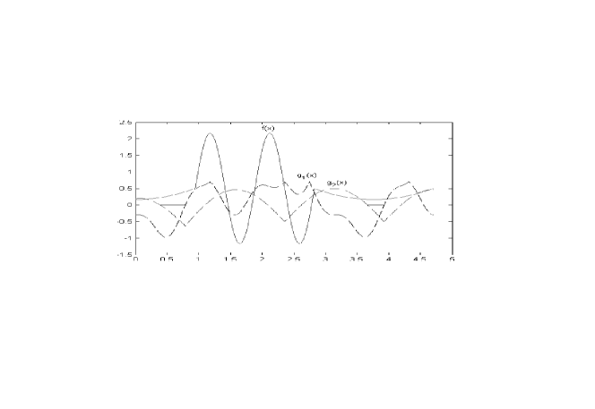
Figure 1: Problem number 6 from [2] where functions $f(x)$ and $g_{1}(x),g_{2}(x)$ are defined over the whole search region $[0,1.5\,\pi]$

Problem of the type (1)–(4) considered in this paper and using the same functions $g_{1}(x)$–$g_{3}(x)$ from (6)–(8) is shown in Figure 2. It has the same global minimizer $x^{*}=3.76984$ and is formulated as follows

$$Q_{1}\,=\,[0,1.5\,\pi],\,\,\,\,Q_{2}\,=\,\{x\,\in\,Q_{1}:\,g_{1}(x)\,\leq 0\},$$ (9)

$$Q_{3}\,=\,\{x\,\in\,Q_{2}:\,g_{2}(x)\,\leq 0\},$$ (10)

$$g_{3}^{*}=g_{3}(x^{*})=\min\{g_{3}(x):x\in Q_{3}\}.$$ (11)

It can be seen from Figure 2 that both $g_{2}(x)$ and $f(x)$ are partially defined: $g_{2}(x)$ is defined only over $Q_{2}$ and the objective function $f(x)$ is defined only over $Q_{3}$ which coincides with the admissible region of problem (5)–(8).

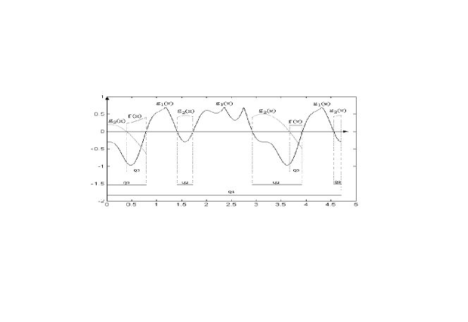
Figure 2: Graphical representation of problem (9)–(11)

It is not easy to find a traditional algorithm for solving problem (1)–(4). For example, the penalty approach requires that $f(x)$ and $g_{i}(x),\,1\leq i\leq m,$ are defined over the whole search interval $[a,b]$. At first glance it seems that at the regions where a function is not defined it can be simply filled in with either a big number or the function value at the nearest feasible point. Unfortunately, in the context of Lipschitz algorithms, incorporating such ideas can lead to infinitely high Lipschitz constants, causing degeneration of the methods and non-applicability of the penalty approach.

A promising approach called the index scheme has been proposed in [13] (see also [11, 14, 15]) in combination with information stochastic Bayesian algorithms for solving problem (1)–(4). An important advantage of the index scheme is that it does not introduce additional variables and/or parameters as traditional approaches do (see, e.g, [1, 3, 4]). It has been recently shown in [10] that the index scheme can be also successfully used in combination with the Branch-and-Bound approach if the Lipschitz constants $L_{j},1\leq j\leq m+1,$ from (3), (4) are known a priori.

However, in practical applications (see, e.g. [6]) the Lipschitz constants $L_{j},1\leq j\leq m+1,$ are very often unknown. Thus, the problem of their estimating arises inevitably. If there exists an additional information allowing us to obtain a priori fixed constants $K_{j}$, $1\leq j\leq m+1$, such that

$$L_{j}<K_{j}<\infty,\hskip 8.53581pt1\leq j\leq m+1,$$

then the algorithm IBBA from [10] can be used.

In this paper, the case where there is no any additional information about the Lipschitz constants is considered. A new GO Algorithm with Local Tuning (ALT) adaptively estimating the local Lipschitz constants during the search is proposed. The local tuning technique introduced in [7, 8, 9] for solving unconstrained problems allows one to accelerate the search significantly in comparison with the methods using estimates of the global Lipschitz constant. The new method ALT unifies this approach with the index scheme and geometric ideas allowing one to construct auxiliary functions similar to minorants used in the IBBA (see [10]). In a series of numerical experiments it is shown that usage of adaptive local estimates calculated during the search instead of a priori given estimates of global Lipschitz constants accelerates the search significantly.

2 A New Geometric Index Algorithm with Local Tuning

Let us associate with every point of the interval $[a,b]$ an index

$$\nu\,=\,\nu(x),\,\,\,\,1\,\leq\nu\,\leq M,$$

which is defined by the conditions

$$g_{j}(x)\,\leq 0,\,\,\,\,1\,\leq j\,\leq\,\nu\,-\,1,\,\,\,\,\,g_{\nu}(x)\,>\,0,$$ (12)

where for $\nu\,=\,m+1$ the last inequality is omitted. We shall call a trial the operation of evaluation of the functions $g_{j}(x),\,1\,\leq\,j\,\leq\,\nu(x)$, at a point $x$.

Thus, the index scheme considers constraints one at a time at every point where it has been decided to try to calculate the objective function $g_{m+1}(x)$. Each constraint $g_{i}(x)$ is evaluated at a point $x$ only if all the inequalities

$$g_{j}(x)\,\leq 0,\,\,\,\,1\,\leq j\,<i,$$

have been satisfied at this point. In its turn the objective function  $g_{m+1}(x)$ is computed only for those points where all the constraints have been satisfied.

Suppose now that $k+1$, $k\geq 1$, trials have been executed at some points

$$a=x_{0}<x_{1}<\ldots<x_{i}<\ldots<x_{k}=b$$ (13)

and the index  $\nu_{i}=\nu(x_{i}),\,\,0\leq i\leq k,$  have been calculated following $(\ref{7})$. Due to the index scheme, the estimate

$$z^{*}_{k}=\displaystyle\ \min\,\{g_{M^{k}}(x_{i}):\,0\leq i\leq k,\,\nu(x_{i})=M^{k}\}$$ (14)

of the minimal value of the function $g_{M^{k}}(x)$ found after $k$ iterations can be calculated and the values

$$z_{i}=g_{\nu(x_{i})}(x_{i})-\left\{\begin{array}[]{cl}0,&\hskip 5.69054pt\mbox{if}\,\,\,\nu(x_{i})<M^{k}\\ z^{*}_{k},&\hskip 5.69054pt\mbox{if}\,\,\,\nu(x_{i})=M^{k}\\ \end{array}\right.$$ (15)

can be associated with the points $x_{i}$ from (13).

In the new algorithm ALT, we propose to adaptively estimate at each iteration the local Lipschitz constants over subintervals $[x_{i-1},x_{i}]\subset[a,b]$, $1\leq i\leq k$, by using the information obtained from executing trials at the points $x_{i}$, $0\leq i\leq k$, from (13). Particularly, at each point $x_{i}$, $0\leq i\leq k,$ having the index $\nu_{i}$ we calculate a local estimate $\eta_{i}$ of the Lipschitz constant $L_{\nu_{i}}$ at a neighborhood of the point $x_{i}$ as follows

$$\eta_{i}=\max\{\lambda_{i},\gamma_{i},\xi\},\hskip 14.22636pt0\leq i\leq k.$$ (16)

Here, $\xi>0$ is a small number reflecting our supposition that the objective function and constraints are not just constants over $[a,b]$, i.e., $L_{j}\geq\xi$, $1\leq j\leq m+1$. The values $\lambda_{i}$ are calculated as follows

$$\small{\lambda_{i}=\left\{\begin{array}[]{ll}\max\{\mid z_{j}-z_{j-1}\mid(x_{j}-x_{j-1})^{-1}:\,\,j=i,i+1\},&\mbox{if}\,\,\nu_{i-1}=\nu_{i}=\nu_{i+1}\\ &\\ \max\{\mid z_{i}-z_{i-1}\mid(x_{i}-x_{i-1})^{-1},\,\,\,z_{i}(x_{i+1}-x_{i})^{-1}\},&\mbox{if}\,\,\nu_{i-1}=\nu_{i}<\nu_{i+1}\\ &\\ \max\{\mid z_{i+1}-z_{i}\mid(x_{i+1}-x_{i})^{-1},\,\,\,z_{i}(x_{i}-x_{i-1})^{-1}\},&\mbox{if}\,\,\nu_{i-1}>\nu_{i}=\nu_{i+1}\\ &\\ \max\{z_{i}(x_{i}-x_{i-1})^{-1},\,\,\,z_{i}(x_{i+1}-x_{i})^{-1}\},&\mbox{if}\,\,\nu_{i}<\nu_{i-1},\,\,\nu_{i}<\nu_{i+1}\\ &\\ z_{i}(x_{i}-x_{i-1})^{-1},&\mbox{if}\,\,\nu_{i-1}>\nu_{i}>\nu_{i+1}\\ &\\ z_{i}(x_{i+1}-x_{i})^{-1},&\mbox{if}\,\,\nu_{i-1}<\nu_{i}<\nu_{i+1}\\ &\\ \mid z_{i}-z_{i-1}\mid(x_{i}-x_{i-1})^{-1},&\mbox{if}\,\,\nu_{i-1}=\nu_{i}>\nu_{i+1}\\ &\\ \mid z_{i+1}-z_{i}\mid(x_{i+1}-x_{i})^{-1},&\mbox{if}\,\,\nu_{i-1}<\nu_{i}=\nu_{i+1}\\ &\\ 0,&\mbox{otherwise}\\ \end{array}\right.}$$ (17)

where $z_{i}$, $0\leq i\leq k$, are from (15). Naturally, when $i=0$ or $i=k$, only one of the two expressions in the first four cases are defined and are used to calculate $\lambda_{i}$. The values $\gamma_{i}$, $0\leq i\leq k,$ are calculated in the following way:

$$\gamma_{i}=\Lambda_{\nu_{i}}\max\{x_{i}-x_{i-1},x_{i+1}-x_{i}\}/X_{\nu_{i}}^{\max},$$ (18)

$$\Lambda_{\nu_{i}}=\Lambda_{\nu_{i}}(k)=\max\{\Lambda_{\nu_{i}}(k-1),\max\{\lambda_{j}:\nu_{j}=\nu_{i},\,0\leq j\leq k\}\},$$ (19)

where $\Lambda_{\nu_{i}}$ are adaptive estimates of the global Lipschitz constants $L_{\nu_{i}}$ and

$$X_{\nu_{i}}^{\max}\,=\,\max\{x_{j}\,-\,x_{j-1}\,:\,\nu_{j}=\nu_{i}\,\,{\rm or}\,\,\nu_{j-1}=\nu_{i},\,\,1\leq j\leq k\}.$$ (20)

The values $\lambda_{i}$ and $\gamma_{i}$ reflect the influence on $\eta_{i}$ of the local and global information obtained during the previous iterations. When both intervals $[x_{i-1},x_{i}]$ and $[x_{i},x_{i+1}]$ are small, then $\gamma_{i}$ is small too (see (18)) and, due to (16), the local information represented by $\lambda_{i}$ has major importance. The value $\lambda_{i}$ is calculated by considering the intervals $[x_{i-2},x_{i-1}],\;[x_{i-1},x_{i}],$ and $[x_{i},x_{i+1}]$ (see (17)) as those which have the strongest influence on the local estimate at the point $x_{i}$ and, in general, at the interval $[x_{i-1},x_{i}]$. When at least one of the intervals $[x_{i-1},x_{i}]$, $[x_{i},x_{i+1}]$ is very wide, the local information is not reliable and, due to (16), the global information represented by $\gamma_{i}$ has the major influence on $\eta_{i}$. Thus, local and global information are balanced in the values $\eta_{i}$, $0\leq i\leq k$. Note that the method uses the local information over the whole search region $[a,b]$ during the global search both for the objective function and constraints.

We are ready now to describe the new algorithm ALT.

Step 0 (Initialization).

Suppose that $k+1$, $k\geq 1$, trails have been already executed in a way at points

$$x^{0}=a,x^{1}=b,x^{2},x^{3},...,x^{i},...x^{k-1},x^{k}$$ (21)

and their indexes and the value

$$M^{k}=\max\{\nu(x^{i}):0\leq\,i\,\leq\,k\}$$ (22)

have been calculated. The value $M^{k}$ defined in (22) is the maximal index obtained during the search after $k+1$ trials. The choice of the point $x^{k+1}$, $k\geq\,1$, where the next trial will be executed is determined by the rules presented below.

Step 1.

Renumber the points $x^{0},....,x^{k}$ of the previous $k$ iterations by subscripts in order to form the sequence (13).

Step 2.

Recalculate the estimate $z^{*}_{k}$ of the minimal value of the function $g_{M^{k}}(x)$ found after $k$ iterations and the values $z_{i}$ by using formulae (14) and (15), respectively. For each trial point $x_{i}$ having the index $\nu_{i}$, $0\leq i\leq k$, calculate estimate $\eta_{i}$ from (16).

Step 3.

For each interval $[x_{i-1},x_{i}],\,1\leq i\leq k$, calculate the characteristic of the interval

$$R_{i}=\left\{\begin{array}[]{ll}(\frac{1}{\eta_{i}+\eta_{i-1}})\left[\eta_{i}z_{i-1}+\eta_{i-1}z_{i}+r\eta_{i-1}\eta_{i}(x_{i-1}-x_{i})\right],&\,\nu_{i-1}\,=\,\nu_{i}\\ z_{i}-r\eta_{i}(x_{i}-x_{i-1}\,-z_{i-1}/r\eta_{i-1}),&\,\nu_{i-1}<\,\nu_{i}\\ z_{i-1}-r\eta_{i-1}(x_{i}-x_{i-1}\,-z_{i}/r\eta_{i}),&\,\nu_{i-1}>\,\nu_{i}\\ \end{array}\right.$$ (23)

where $r>1$ is the reliability parameter of the method (this kind of parameters is quite traditional in Lipschitz global optimization; discussions related to its choice and meaning can be found in [6, 12, 15]).

Step 4.

Find an interval $t$ corresponding to the minimal characteristic, i.e.,

$$t=\arg\min\{\,R_{i}:\,1\leq i\leq k\}.$$ (24)

If the minimal value of the characteristic is attained for several subintervals, then the minimal integer satisfying (24) is accepted as $t$.

Step 5.

If for the interval $[x_{t-1},x_{t}],$ where $t$ is from (24), the stoping rule

$$x_{t}-x_{t-1}\leq\varepsilon(b-a),$$ (25)

where $a$ and $b$ are from (1)–(4), is satisfied for a preset accuracy $\varepsilon>0$, then Stop – the required accuracy has been reached. In the opposite case, go to Step 6.

Step 6.

Execute the $(k+1)$-th trial at the point

$$x^{k+1}=\left\{\begin{array}[]{ll}(\frac{1}{r\eta_{t}+r\eta_{t-1}})\left[z_{t-1}-z_{t}+r\eta_{t-1}x_{t-1}+r\eta_{t}x_{t}\right],&{\rm if}\,\nu_{i-1}=\,\nu_{i}\\ 0.5(x_{t-1}+x_{t}),&{\rm if}\,\nu_{i-1}\neq\nu_{i},\end{array}\right.$$ (26)

and evaluate its index $\nu(x^{k+1})$.

Step 7.

This step consists of the following alternatives:

Case 1. If $\nu(x^{k+1})>M^{k}$, then perform two additional trials at the points

$$x^{k+2}=0.5(x_{t-1}+x^{k+1}),\hskip 28.45274ptx^{k+3}=0.5(x^{k+1}+x_{t}),$$ (27)

calculate their indexes, set $k=k+3$, and go to Step 8.

Case 2. If $\nu(x^{k+1})<M^{k}$ and among the points (13) there exists only one point $x_{T}$ with the maximal index $M^{k}$, i.e., $\nu_{T}=M^{k}$, then execute two additional trials at the points

$$x^{k+2}=0.5(x_{T-1}+x_{T}),$$ (28)

$$x^{k+3}=0.5(x_{T}+x_{T+1}),$$ (29)

if $0<T<k$, calculate their indexes, set $k=k+3$, and go to Step 8. If $T=0$ then the trial is executed only at the point (29). Analogously, if $T=k$ then the trial is executed only at the point (28). In these two cases, calculate the index of the additional point, set $k=k+2$ and go to Step 8.

Case 3. In all the remaining cases set $k=k+1$ and go to Step 8.

Step 8.

Calculate $M^{k}$ and go to Step 1.

Global convergence conditions of the ALT are described by the following two theorems given, due to the lack of space, without proofs that can be derived using Theorems 2 and 3 from [8] and Theorem 2 from [10].

Theorem 2.1

Let the feasible region $Q_{m+1}\neq\varnothing$ consists of intervals having finite lengths, $x^{*}$ be any solution to problem (1)–(4), and $j=j(k)$ be the number of an interval $[x_{j-1},x_{j}]$ containing this point during the $k$-th iteration. Then, if for $k\geq k^{*}$ the following conditions

$$r\Lambda_{\nu_{j-1}}>C_{j-1},\hskip 14.22636ptr\Lambda_{\nu_{j}}>C_{j},$$ (30)

$$C_{j-1}=z_{j-1}/(x^{*}-x_{j-1}),\hskip 14.22636ptC_{j}=z_{j}/(x_{j}-x^{*}).$$ (31)

take place, then the point $x^{*}$ will be a limit point of the trial sequence $\{x^{k}\}$ generated by the ALT.

Theorem 2.2

For any problem (1)–(4) there exists a value $r^{*}$ such that conditions (30) are satisfied for all parameters $r>r^{*},$ where $r$ is from (23) and (26).

3 Numerical Comparison

The new algorithm has been numerically compared with the following methods:

–

The method proposed by Pijavskii (see [3, 5]) combined with the penalty approach used to reduce the constrained problem to an unconstrained one; this method is indicated hereafter as PEN. The Lipschitz constant of the obtained unconstrained problem is supposed to be known as it is required by Pijavskii algorithm.

–

The method IBBA from [10] using the index scheme in combination with the Branch-and-Bound approach and the known Lipschitz constants $L_{j},1\leq j\leq m+1,$ from (3), (4).

Ten non-differentiable test problems introduced in [2] have been used in the experiments (since there were several misprints in the original paper [2], the accurately verified formulae have been applied, which are available at the Web-site http://wwwinfo.deis.unical.it/$\sim$yaro/constraints.html). In this set of tests, problems 1–3 have one constraint, problems 4–7 two constraints, and problems 8–10 three constrains.

In these test problems, all constrains and the objective function are defined over the whole region $[a,b]$ from (2). These test problems were used because the PEN needs this additional information for its work and is not able to solve problem (1)–(4). Naturally, the methods IBBA and ALT solved all the problems using the statement (1)–(4) and did not take benefits from the additional information given (see examples from Figures 1 and 2) by the statement (5)–(8) in comparison with (9)–(11).

In order to demonstrate the influence of changing the search accuracy $\varepsilon$ on the convergence speed of the methods, two different values of $\varepsilon$, namely, $\varepsilon=10^{-4}$ and $\varepsilon=10^{-5}$ have been used. The same value $\xi=10^{-6}$ from (16) has been used in all the experiments for all the methods.

Table 1 represents the results for the PEN (see [2]). The constrained problems were reduced to the unconstrained ones as follows

$$f_{P^{*}}(x)=f(x)+P^{*}\max\left\{0,g_{1}(x),g_{2}(x),\dots,g_{N_{v}}(x)\right\}.$$ (32)

The column “Eval.” in Table 1 shows the total number of evaluations of the objective function $f(x)$ and all the constraints. Thus, it is equal to

$$(N_{v}+1)\times N_{trials},$$

where $N_{v}$ is the number of constraints and $N_{trials}$ is the number of the trials executed by the PEN for each problem.

Results obtained by the IBBA (see [10]) and by the new method ALT with the parameter $r=1.3$ are summarized in Tables 4 and  4, respectively. Columns in the tables have the following meaning for each value of the search accuracy $\varepsilon$:

$-$the column $\mathcal{N}$ indicates the problem number;

$-$the columns $N_{g_{1}},N_{g_{2}},$ and $N_{g_{3}}$ represent the number of trials where the constraint $g_{i},\,1\leq i\leq 3$, was the last evaluated constraint;

$-$the column “Trials” is the total number of trial points generated by the methods;

$-$the column “Eval.” is the total number of evaluations of the objective function and the constraints. This quantity is equal to:

$-$$N_{g_{1}}+2\times N_{f}$, for problems with one constraint;

$-$$N_{g_{1}}+2\times N_{g_{2}}+3\times N_{f}$, for problems with two constraints;

$-$$N_{g_{1}}+2\times N_{g_{2}}+3\times N_{g_{3}}+4\times N_{f}$, for problems with three constraints.

Table 1: Numerical results obtained by the PEN

$\mathcal{N}$	$P^{*}$	$\varepsilon=10^{-4}$		$\varepsilon=10^{-5}$
		Trials	Eval.	Trials	Eval.
1	$15$	$247$	$494$	$419$	$838$
2	$15$	$241$	$482$	$313$	$626$
3	$15$	$917$	$1834$	$2127$	$4254$
4	$15$	$273$	$819$	$861$	$2583$
5	$20$	$671$	$2013$	$1097$	$3291$
6	$15$	$909$	$2727$	$6367$	$19101$
7	$15$	$199$	$597$	$221$	$663$
8	$15$	$365$	$1460$	$415$	$1660$
9	$15$	$1183$	$4732$	$4549$	$18196$
10	$15$	$135$	$540$	$169$	$676$
Av.	$-$	$514.0$	$1569.8$	$1653.8$	$5188.8$

The asterisk in Table 4 indicates that $r=1.3$ was not sufficient to find the global minimizer of problem 7. The results for this problem in Table 4 are obtained using the value $r=1.9$; the ALT with this value finds the solution. Finally, Table 4 represents the improvement (in terms of the number of trials and evaluations) obtained by the ALT in comparison with the other methods used in the experiments.

As it can be seen from Tables 1–4, the algorithms IBBA and ALT constructed in the framework of the index scheme significantly outperform the traditional method PEN. The ALT demonstrates a high improvement in terms of the trials performed with respect to the IBBA as well. In particular, the greater the difference between estimates of the local Lipschitz constants (for the objective function or for the constraints), the higher is the speed up obtained by the ALT (see Table 4). The improvement is especially high if the global minimizer lies inside of a feasible subregion with a small (with respect to the global Lipschitz constant) value of the local Lipschitz constant as it happens for example for problems 6 and 9. The advantage of the new method is more pronounced when the search accuracy $\varepsilon$ increases (see Table 4).

Table 2: Numerical results obtained by the IBBA

$\mathcal{N}$	$\varepsilon=10^{-4}$						$\varepsilon=10^{-5}$
	$N_{g_{1}}$	$N_{g_{2}}$	$N_{g_{3}}$	$N_{f}$	Trials	Eval.	$N_{g_{1}}$	$N_{g_{2}}$	$N_{g_{3}}$	$N_{f}$	Trials	Eval.
1	$23$	$-$	$-$	$28$	$51$	$79$	$23$	$-$	$-$	$34$	$57$	$91$
2	$18$	$-$	$-$	$16$	$34$	$50$	$20$	$-$	$-$	$22$	$42$	$64$
3	$171$	$-$	$-$	$19$	$190$	$209$	$175$	$-$	$-$	$21$	$196$	$217$
4	$136$	$15$	$-$	$84$	$235$	$418$	$170$	$15$	$-$	$226$	$411$	$878$
5	$168$	$91$	$-$	$24$	$283$	$422$	$188$	$101$	$-$	$26$	$315$	$468$
6	$16$	$16$	$-$	$597$	$629$	$1839$	$17$	$17$	$-$	$2685$	$2719$	$8106$
7	$63$	$18$	$-$	$39$	$120$	$216$	$65$	$19$	$-$	$43$	$127$	$232$
8	$29$	$11$	$3$	$21$	$64$	$144$	$29$	$14$	$3$	$23$	$69$	$158$
9	$8$	$86$	$57$	$183$	$334$	$1083$	$10$	$88$	$57$	$851$	$1006$	$3761$
10	$42$	$3$	$17$	$13$	$75$	$151$	$42$	$3$	$17$	$15$	$77$	$159$
Av.	$-$	$-$	$-$	$-$	$201.5$	$461.1$	$-$	$-$	$-$	$-$	$501.9$	$1413.4$

Table 3: Numerical results obtained by the ALT with $r=1.3$

$\mathcal{N}$	$\varepsilon=10^{-4}$						$\varepsilon=10^{-5}$
	$N_{g_{1}}$	$N_{g_{2}}$	$N_{g_{3}}$	$N_{f}$	Trials	Eval.	$N_{g_{1}}$	$N_{g_{2}}$	$N_{g_{3}}$	$N_{f}$	Trials	Eval.
1	$27$	$-$	$-$	$17$	$44$	$61$	$27$	$-$	$-$	$19$	$46$	$65$
2	$19$	$-$	$-$	$15$	$34$	$49$	$22$	$-$	$-$	$16$	$38$	$54$
3	$12$	$-$	$-$	$9$	$21$	$30$	$14$	$-$	$-$	$10$	$24$	$34$
4	$45$	$11$	$-$	$37$	$93$	$178$	$45$	$11$	$-$	$48$	$104$	$211$
5	$73$	$44$	$-$	$15$	$132$	$206$	$76$	$44$	$-$	$17$	$137$	$215$
6	$21$	$11$	$-$	$42$	$74$	$169$	$21$	$11$	$-$	$64$	$96$	$235$
7∗	$34$	$27$	$-$	$39$	$100$	$205$	$34$	$34$	$-$	$42$	$110$	$228$
8	$12$	$20$	$4$	$23$	$59$	$156$	$12$	$22$	$4$	$24$	$62$	$164$
9	$8$	$16$	$3$	$29$	$56$	$165$	$8$	$16$	$3$	$36$	$63$	$193$
10	$14$	$2$	$13$	$13$	$42$	$109$	$14$	$2$	$13$	$18$	$47$	$129$
Av.	$-$	$-$	$-$	$-$	$65.5$	$132.8$	$-$	$-$	$-$	$-$	$72.7$	$152.8$

Table 4: Improvement obtained by the ALT with $r=1.3$ in comparison with the other methods used in the experiments

$\mathcal{N}$	$\varepsilon=10^{-4}$				$\varepsilon=10^{-5}$
	Trials		Eval.		Trials		Eval.
	$\frac{\mbox{PEN}}{\mbox{ALT}}$	$\frac{\mbox{IBBA}}{\mbox{ALT}}$	$\frac{\mbox{PEN}}{\mbox{ALT}}$	$\frac{\mbox{IBBA}}{\mbox{ALT}}$	$\frac{\mbox{PEN}}{\mbox{ALT}}$	$\frac{\mbox{IBBA}}{\mbox{ALT}}$	$\frac{\mbox{PEN}}{\mbox{ALT}}$	$\frac{\mbox{IBBA}}{\mbox{ALT}}$
1	$5.61$	$1.16$	$8.10$	$1.30$	$9.11$	$1.24$	$12.89$	$1.40$
2	$7.09$	$1.00$	$9.84$	$1.02$	$8.24$	$1.11$	$11.59$	$1.19$
3	$43.67$	$9.05$	$61.13$	$6.97$	$88.63$	$8.17$	$125.12$	$6.38$
4	$2.94$	$2.53$	$4.60$	$2.35$	$8.28$	$3.95$	$12.24$	$4.16$
5	$5.08$	$2.14$	$9.77$	$2.05$	$8.01$	$2.30$	$15.31$	$2.18$
6	$12.28$	$8.50$	$16.14$	$10.88$	$66.32$	$28.32$	$81.28$	$34.49$
7∗	$1.99$	$1.20$	$2.91$	$1.05$	$2.01$	$1.15$	$2.91$	$1.02$
8	$6.19$	$1.08$	$9.36$	$0.92$	$6.69$	$1.11$	$10.12$	$0.96$
9	$21.13$	$5.96$	$28.68$	$6.56$	$72.21$	$15.97$	$94.28$	$19.49$
10	$3.21$	$1.79$	$4.95$	$1.39$	$3.60$	$1.64$	$5.24$	$1.23$
Av.	$10.92$	$3.44$	$15.55$	$3.45$	$27.31$	$6.50$	$37.10$	$7.25$

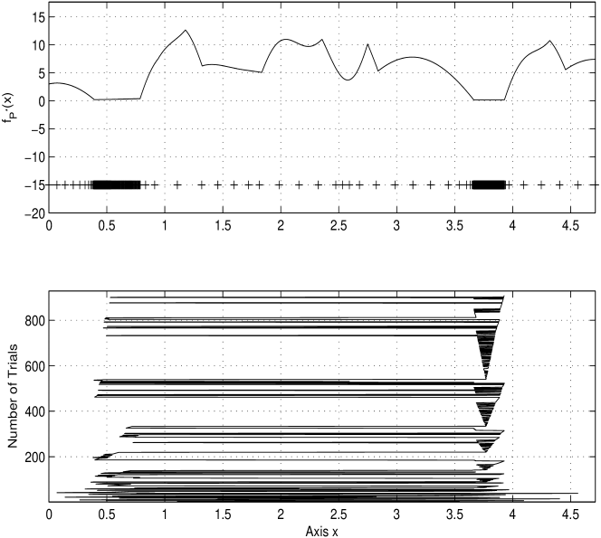
Figure 3: Solving by the method PEN the unconstrained problem (32) constructed from the problem (5)–(8) shown in Figure 1

In order to illustrate performance of the methods graphically, in Figures 3–5 we show dynamic diagrams of the search (with the accuracy $\varepsilon=10^{-4}$ in (25)) executed by the PEN, the IBBA, and the ALT, respectively, for problem 6 from [2]. The upper subplot of Figure 3 contains the function $f_{P^{*}}(x)$ from (32) constructed from the problem (5)–(8) shown in Figure 1. The upper subplots of Figures 5 and 5 contain the index function (see [10, 15] for a detailed discussion) corresponding to the problem (9)–(11) from Figure 2. Note that the local Lipschitz constant corresponding to the objective function over this subregion is significantly smaller than the global one (see Figures 2 and 5).

The line of symbols ‘+’ located under the graph of the function (32) in Figure 3 shows points at which trials have been executed by the PEN. The lower subplots show dynamics of the search. The PEN has executed 909 trials and the number of evaluations was equal to $909\times 3=2727$. In Figure 5 the first line (from up to down) of symbols ‘+’, located under the graph of problem (9)–(11), represents the points where the first constraint has not been satisfied (number of such trials is equal to 16). Thus, due to the decision rule of the IBBA, the second constraint has not been evaluated at these points.

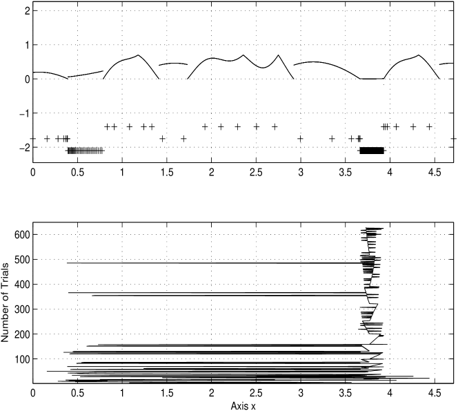
Figure 4: Solving the problem (9)–(11) by the method IBBA

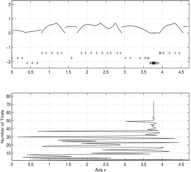
Figure 5: Solving the problem (9)–(11) by the method ALT with $r=1.3$

The second line of symbols ‘+’ represents the points where the first constraint has been satisfied but the second constraint has been not (number of such trials is equal to 16). At these points both constraints have been evaluated but the objective function has been not. The last line represents the points where both constraints have been satisfied (number of such trials is 597) and, therefore, the objective function has been evaluated too. The total number of evaluations is equal to $16+16\times 2+597\times 3=1839$. These evaluations have been executed during $16+16+597=629$ trials.

Similarly, in Figure 5, the first line of symbols ‘+’ indicates 21 trial points where the first constraint has not been satisfied. The second line represents 11 points where the first constraint has been satisfied but the second constraint has been not. The last line shows 42 points where both constraints have been satisfied and the objective function has been evaluated. The total number of evaluations is equal to $21+11\times 2+42\times 3=169$. These evaluations have been executed during $21+11+42=74$ trials.

References

• [1] Bertsekas D.P. (1996), Constrained Optimization and Lagrange Multiplier Methods, Athena Scientific, Belmont, MA.
• [2] Famularo D., Sergeyev Ya.D., and Pugliese P. (2002), Test Problems for Lipschitz Univariate Global Optimization with Multiextremal Constraints. In: Dzemyda G., Šaltenis V., and Žilinskas A. (Eds.). Stochastic and Global Optimization, Kluwer Academic Publishers, Dordrecht, 93–110.
• [3] Horst R. and Pardalos P.M. (1995), Handbook of Global Optimization, Kluwer Academic Publishers, Dordrecht.
• [4] Nocedal J. and Wright S.J. (1999), Numerical Optimization (Springer Series in Operations Research), Springer Verlag.
• [5] Pijavskii S.A. (1972), An Algorithm for Finding the Absolute Extremum of a Function, USSR Comput. Math. Math. Phys., 12 57–67.
• [6] Pintér J.D. (1996), Global Optimization in Action, Kluwer Academic Publisher, Dordrecth.
• [7] Sergeyev Ya.D. (1995a) An information global optimization algorithm with local tuning, SIAM J. Optim. 5, 858–870.
• [8] Sergeyev Ya.D. (1995b) A one-dimensional deterministic global minimization algorithm, Comput. Math. Math. Phys. 35, 705–717.
• [9] Sergeyev Ya.D. (1998), Global one-dimensional optimization using smooth auxiliary functions, Math. Program., 81, 127–146.
• [10] Sergeyev Ya.D., Famularo D., and Pugliese P. (2001), Index Branch-and-Bound Algorithm for Lipschitz Univariate Global Optimization with Multiextremal Constraints, J. Global Optim., 21, 317–341.
• [11] Sergeyev Ya.D. and Markin D.L. (1995), An algorithm for solving global optimization problems with nonlinear constraints, J. Global Optim., 7, 407–419.
• [12] Strongin R.G. (1978), Numerical Methods on Multiextremal Problems, Nauka, Moscow. (In Russian).
• [13] Strongin, R.G. (1984), Numerical methods for multiextremal nonlinear programming problems with nonconvex constraints. In: Demyanov V.F. and Pallaschke D. (Eds.). Lecture Notes in Economics and Mathematical Systems 255, Proceedings 1984. Springer-Verlag. IIASA, Laxenburg/Austria, 278–282.
• [14] Strongin R.G. and Markin D.L. (1986), Minimization of multiextremal functions with nonconvex constraints, Cybernetics, 22, 486–493.
• [15] Strongin R.G. and Sergeyev Ya.D. (2000), Global Optimization with Non-Convex Constraints: Sequential and Parallel Algorithms, Kluwer Academic Publishers, Dordrecht.