Univariate global optimization with multiextremal non-differentiable constraints without penalty functions

Abstract

This paper proposes a new algorithm for solving constrained global optimization problems where both the objective function and constraints are one-dimensional non-differentiable multiextremal Lipschitz functions. Multiextremal constraints can lead to complex feasible regions being collections of isolated points and intervals having positive lengths. The case is considered where the order the constraints are evaluated is fixed by the nature of the problem and a constraint $i$ is defined only over the set where the constraint $i-1$ is satisfied. The objective function is defined only over the set where all the constraints are satisfied. In contrast to traditional approaches, the new algorithm does not use any additional parameter or variable. All the constraints are not evaluated during every iteration of the algorithm providing a significant acceleration of the search. The new algorithm either finds lower and upper bounds for the global optimum or establishes that the problem is infeasible. Convergence properties and numerical experiments showing a nice performance of the new method in comparison with the penalty approach are given.

Key Words: Global optimization, multiextremal constraints, Lipschitz functions,
continuous index functions.

1 Introduction

In last decades univariate global optimization problems were studied intensively (see [7, 15, 18, 19, 22, 28, 31, 37, 43]) because there exists a large number of real-life applications where it is necessary to solve such problems (see [6, 15, 27, 30, 33, 37, 40]). On the other hand, it is important to study these problems because mathematical approaches developed to solve them can be generalized to the multidimensional case by numerous schemes (see, for example, one-point based, diagonal, simplicial, space-filling curves, and other popular approaches in [14, 16, 17, 23, 26, 29, 37]).

Electrotechnics and electronics are among the fields where one-dimensional global optimization methods can be used successfully (see [8, 9, 10, 11, 24, 33, 40]). Let us consider, for example, the following so-called ‘mask problem’ for transmitters. We have a transmitter (for instance, that of GSM cellular phones) that in a frequency interval $[a,b]$ has an amplitude $A(x)$ that should be inside the mask defined by functions $l(x)$ and $u(x)$, i.e., it should be $l(x)\leq A(x)\leq u(x)$. The mask is defined by international rules agreed to avoid interference appearing when amplitude is too high for a given frequency and by properties of electronic components used to construct the transmitter. Then, it is necessary to find a frequency $x^{*}\in[a,b]$ such that the power, $p(x)$, of the transmitted signal is maximal.

It happens often in engineering optimization problems (see [37, 40]) that if a constrained is not satisfied at a point then many other constraints and the objective function are not defined at this point. This situation holds in our mask problem because if for a frequency $\xi$ if happens that $A(\xi)>u(\xi)$ or $A(\xi)<l(\xi)$ then there is no transmission and the function $p(\xi)$ is not defined. Since the amplitude can touch the mask both from its internal and its external parts, isolated points in the admissible region of $p(x)$ can take place. If the maximal power $p(x^{*})$ is attained at an isolated point $x^{*}$, then this point should be discarded from consideration because it cannot be realized in practice. Thus, the solution is acceptable only if it belongs to a finite interval of a certain length.

This problem can be reformulated in the following general framework of global optimization problems considered in this paper. It is necessary to find the global minimizers and the global minimum of a function $f(x)$ subject to constraints $g_{j}(x)\leq 0,1\leq i\leq m,$ over an interval $[a,b]$. The objective function $f(x)$ and constraints $g_{j}(x),1\leq i<m,$ are multiextremal non-differentiable ‘black-box’ Lipschitz functions with a priori known Lipschitz constants (to unify the description process the designation $g_{m+1}(x)\triangleq f(x)$ is used hereinafter). Very often in real-life applications the order the constraints are evaluated is fixed by the nature of the problem and not all the constraints are defined over the whole search region $[a,b]$. The worst case is considered here, i.e., a constraint $g_{j+1}(x)$ is defined only over subregions where $g_{j}(x)\leq 0$. This means that if a constraint is not satisfied at a point, the rest of constraints and the objective function are not defined at that point. The sets $Q_{j},1\leq j\leq m+1,$ can be so defined as follows

$$Q_{1}=[a,b],\hskip 8.53581ptQ_{j+1}=\{x\in Q_{j}:g_{j}(x)\leq 0\},\hskip 14.22636pt1\leq j\leq m,$$ (1)

$$Q_{1}\supseteq Q_{2}\supseteq\ldots\supseteq Q_{m}\supseteq Q_{m+1}.$$

Since the constraints are multiextremal, the admissible region $Q_{m+1}$ and regions $Q_{j},$ $1\leq j\leq m,$ can be collections of intervals having positive lengths and isolated points. Particularly, isolated points appear when one of the constraints touches zero, for example, if $g_{j}(x)$ is the square of some function, then $g_{j}(x)\leq 0$ only when $g_{j}(x)=0$. To be implementable in practice, optimal solutions should have a feasible neighborhood of positive length thus, an additional constraint is included in the model: a point $x^{*}$ should belong to an admissible interval having length equal to or greater than $\delta>0$ – a value supplied by the final user. The set of all such intervals is designated as $Q^{\delta}$ (of course, $Q^{\delta}\subseteq Q_{m+1}$). Eventually found isolated points and feasible subregions having length less than $\delta$ should be excluded from consideration. If the case of infeasible problem $Q^{\delta}=\emptyset$ holds, it should be also determined.

We can now state the problem formally. Find the global minimizers $x^{*}$ and the corresponding value $f^{*}$ such that

$$f^{*}=f(x^{*})=\min\{f(x):x\in Q^{\delta}\},$$ (2)

where the objective function $f(x)$ and constraints $g_{j}(x),1\leq i<m,$ are multiextremal functions satisfying the Lipschitz condition in the form

$$\mid g_{j}(x^{\prime})-g_{j}(x^{\prime\prime})\mid\leq L_{j}\mid x^{\prime}-x^{\prime\prime}\mid,\hskip 8.53581ptx^{\prime},x^{\prime\prime}\in Q_{j},\hskip 8.53581pt1\leq j\leq m+1,$$ (3)

and the constants

$$0<L_{j}<\infty,\hskip 14.22636pt1\leq j\leq m+1\,,$$ (4)

are known (this supposition is classical in global optimization (see [15, 17, 28])). Methods working on the basis of this assumption are called ‘exact’ in literature, methods estimating these values are ‘practical’. On the one hand, the exact methods serve as a basis for studying theoretical properties of practical ones and are used as a unit of measure of the speed of practical methods. On the other hand, in certain cases, when additional information about the objective function and constraints is available, they can be applied directly.

An example of such a problem is shown in Fig. 1. It has two non-differentiable multiextremal constraints $g_{1}(x)$ and $g_{2}(x)$. The corresponding sets $Q_{1}=[a,b],Q_{2},$ and $Q_{3}$ are shown. The point $c$ belongs to the sets $Q_{1},Q_{2},$ and $Q_{3}$ but $c\notin Q^{\delta}$. The set $Q^{\delta}$ is shown by the grey color. It can be seen from Fig. 1 that the sets $Q_{2},Q_{3},$ and $Q^{\delta}$ consist of disjoint subregions and $Q_{2},Q_{3}$ contain also an isolated point.

Figure 1: An example of the problem (2)–(4).

It is not easy to find a traditional algorithm for solving the problem (2)–(4). For example, the penalty approach requires that $f(x)$ and $g_{i}(x),\,1\leq i\leq m,$ are defined over the whole search interval $[a,b]$. It seems that missing values can be simply filled in with either a big number or the function value at the nearest feasible point. Unfortunately, in the context of Lipschitz algorithms, incorporating such ideas can lead to infinitely high Lipschitz constants, causing degeneration of the methods and non-applicability of the penalty approach.

A promising approach called the index scheme has been proposed in [38] (see also [39, 40]) in combination with stochastic Bayesian algorithms. An important advantage of the index scheme is that it does not introduce additional variables and/or parameters by opposition to classical approaches in [2, 3, 16, 17, 25]. It has been recently shown in [35] that the index scheme can be also successfully used in combination with the Branch-and-Bound approach. Unfortunately, this scheme can not be applied directly for solving the problem (2)–(4) because it has good convergence properties when all the sets $Q_{j},1\leq j\leq m+1,$ have no isolated points – requirement hardly verified in practice without some additional information about the problem.

Thus, isolated points give serious problems when one has only Lipschitz information. First, because it is not possible to say a priori whether the feasible region has isolated points or not (for example, the method from [35] converges only to global minimizers if it is ensured absence of isolated points). Second, in Lipschitz global optimization isolated points can lead to two problems: accumulation of trial points in their neighborhood (this happens even if there exists a sub-region where a constraint does not touch zero but is only close to zero) and increasing the estimates of Lipschitz constants to infinity. This fact means that the search region will be covered by a uniform mesh of trials) if the Lipschitz constant is estimated or the method simply will not work if the Lipschitz constant is given – our case – because local adaptively obtained information will contradict the given one. Therefore, traditional Lipschitz methods cannot be used in the presence of isolated points and, since their absence can be hardly determined in practice, developments of methods that are able to work independently of the presence or absence of them becomes very important.

In this paper, such a method is proposed. It evolves the idea of separate consideration of each constraint introduced in [38] in a new way and reduces the original constrained problem to a new continuous problem. The method from [35] is used as a basis for construction of the new scheme. Instead of discontinuous support functions proposed in [35], new continuous functions are built. These new structures are very important because by using them it becomes possible to apply numerous tools developed in Lipschitz unconstrained optimization to a very general class of constrained problems. It is also necessary to emphasize that the new approach does not introduce additional variables and/or parameters during this passage from initial discontinuous constrained partially defined problem to the continuous unconstrained one.

To conclude this introduction it is necessary to emphasize once again that the problem of multi-dimensional extensions of one-dimensional Lipschitz global optimization methods to many dimensions is a non-trivial serious problem (P. Hansen and B. Jaumard write in their survey on Lipschitz optimization [15] published in the Handbook of Global Optimization: ‘Large problems (with 10 variables or more) appear to be often intractable, at least if high precision is required’) and is beyond the scope of this paper dedicated to the univariate algorithms and univariate applications. However, the approach proposed here is very promising from this point of view. In the future, a number of various multi-dimensional extensions (starting from the adaptive diagonal and space-filling curves approaches (see [34, 40])) of the algorithm presented in this paper will be studied.

The rest of the paper is organized as follows. The new method is described in Section 2. Section 3 contains computational results and a brief conclusion.

2 Continuous index functions and the new algorithm

The index scheme (see [38, 39, 40]) considers constraints one at a time at every point where it has been decided to calculate $f(x)$ determining the index $\nu=\nu(x),1\leq\nu\leq m+1,$ by the following conditions

$$g_{j}(x)\leq 0,\hskip 8.53581pt1\leq j\leq\nu-1,\hskip 14.22636ptg_{\nu}(x)>0,$$ (5)

where for $\nu=m+1$ the last inequality is omitted. The term trial used hereinafter means determining the index $\nu(x)$ at a point $x$ by evaluation $g_{i}(x),1\leq i\leq\nu(x)$. The index $\nu(x)$ and the value $g_{\nu(x)}(x)$ are called results of the trial.

The discontinuous index function $J(x),x\in[a,b],$ can be written for the problem (2)–(4) following [38]

$$J(x)=g_{\nu(x)}(x)-\left\{\begin{array}[]{ll}0\,,&\nu(x)<m+1,\\ f^{*}\,,&\nu(x)=m+1,\end{array}\right.$$ (6)

where the value $f^{*}$ is the unknown solution to this problem.

Let us start our theoretical consideration by noticing that the global minimizer of the original constrained problem (2)–(4) in the case $Q^{\delta}\neq\emptyset$ coincides with the solution to the following unconstrained discontinuous problem

$$J(x^{*})=\min\{J(x):x\in\overline{Q}^{\delta}\},$$ (7)

where

$$\overline{Q}^{\delta}=[a,b]\setminus\{Q_{m+1}\setminus Q^{\delta}\}.$$ (8)

Suppose now that trials have been executed in a way at some points

$$a=x_{0}<x_{1}<\ldots<x_{i}<\ldots<x_{k}=b$$ (9)

and $\nu_{i}=\nu(x_{i}),0\leq i\leq k,$ are their starting indexes. Note that the notion of index is different with respect to [38, 39, 40] where the index is calculated once and then used in the course of optimization. In this paper, formula (5) defines the starting value for the index that can then be changed during the work of the algorithm.

The points from (9) form the list (called hereinafter History List $H(k)$) of intervals $[l_{i},r_{i}],1\leq i\leq k,$ where

$$l_{i}<r_{i},\hskip 14.22636pt1\leq i\leq k,$$

$$r_{i}=l_{i+1},\hskip 14.22636pt1\leq i<k.$$

The record $x\in H(k)$ means that the point $x=l_{i}$ or $x=r_{i}$ for an interval $i$ from $H(k)$. Every element $i,1\leq i\leq k,$ of the list contains the following information:

$$[l_{i},r_{i}],\hskip 5.69054pt\nu(l_{i}),\hskip 5.69054pt\nu(r_{i}),\hskip 5.69054ptg_{\nu(l_{i})}(l_{i}),\hskip 5.69054ptg_{\nu(r_{i})}(r_{i}).$$ (10)

The second list, $W(k)$, called Working List is built during the work of the method to be introduced by excluding from $H(k)$ intervals where global minimizers of the problem (2)–(4) can not be located (initially it is stated $W(k)=H(k)$). In contrast to $H(k)$ where the information (10) is calculated once and then is kept during the search, indexes $\nu(l_{i})$ and $\nu(r_{i})$ in $W(k)$ can be changed in the course of optimization.

In order to pass from the problem (2)–(4) to the problem (7) it is necessary to estimate the value $f^{*}$ from (2) and the set $Q^{\delta}$. Using the results of trials at the points from the row (9) the value

$$Z^{*}_{k}=\min\{g_{m+1}(x):\nu(x)=m+1,x\in W(k)\}.$$ (11)

estimating $f^{*}$ can be calculated if there exist points $x$ with the index $\nu(x)=m+1$. This value allows us to define the function $J^{k}(x),x\in[a,b],$ by replacing the unknown value $f^{*}$ in (6) by $Z^{*}_{k}$:

$$J^{k}(x)=g_{\nu(x)}(x)-\left\{\begin{array}[]{ll}0\,,&\nu(x)<m+1,\\ Z^{*}_{k}\,,&\nu(x)=m+1.\end{array}\right.$$ (12)

The following Lemma establishes some useful properties of the functions $J(x)$ and $J^{k}(x)$.

Lemma 1

The following assertions hold for the functions $J(x)$ and $J^{k}(x)$:

1. for all points $x$ having indexes $\nu(x)<m+1$, it follows $J^{k}(x)=J(x)>0$;

2. $$J^{k}(x)\leq 0,\hskip 14.22636ptx\in\{x:g_{m+1}(x)\leq Z^{*}_{k}\}.$$ (13)

3. if $\nu(x)=m+1$ and $Z^{*}_{k}\geq f^{*}$ then

   $$J^{k}(x)\leq J(x).$$ (14)

Proof. Truth of assertions i – iii follows from definitions of the functions $J(x)$ and $J^{k}(x)$.  

Particularly, it follows from Lemma 1 that (14) holds if the trial point corresponding to $Z^{*}_{k}$ belongs to $Q^{\delta}$. The estimate (14) is not true if $Z^{*}_{k}\leq f^{*}$, the situation which can occur only if $x^{*}_{k}$ belongs to the set $Q_{m+1}\setminus Q^{\delta}$ where

$$x^{*}_{k}=\arg\min\{g_{m+1}(x):\nu(x)=m+1,x\in W(k)\}.$$ (15)

Let us introduce the following continuous index function $C(x),x\in\overline{Q}^{\delta},$ and study its properties.

$$C(x)=\max_{y\in\overline{Q}^{\delta}}\{J(x),\hskip 2.84526ptJ(y)-K_{\nu(y)}\mid x-y\mid)\},$$ (16)

where $K_{\nu(y)}$ such that $L_{\nu(y)}<K_{\nu(y)}<\infty$ is an overestimate of the Lipschitz constant corresponding to the function $g_{\nu(y)}(y)$ and $J(x)$ is the discontinuous index function from (6).

As an illustration, the function $C(x)$ corresponding to the problem presented in Fig. 1 is shown in Fig. 2. The parts of the function $C(x)$ corresponding to $x$ and $y$ such that

$$J(x)<J(y)-K_{\nu(y)}\mid x-y\mid$$

are shown by the thin line.

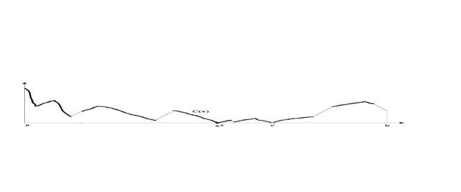
Figure 2: The function $C(x)$ corresponding to the problem presented in Fig. 1.

If $Q^{\delta}\neq\emptyset$, the global minimizers of the original constrained problem (2)–(4) coincide with the solutions of the following continuous problem

$$C(x^{*})=\min\{C(x):x\in\overline{Q}^{\delta}\}.$$ (17)

In the case $Q^{\delta}=\emptyset$ the set $\overline{Q}^{\delta}=[a,b]\setminus\ Q_{m+1}$ and we have $\nu(x)<m+1,x\in\overline{Q}^{\delta}$. Thus, due to Lemma 1, it follows

$$C(x)>0,\hskip 8.53581ptx\in\overline{Q}^{\delta}.$$ (18)

Similarly to definition of the function $J^{k}(x)$, the value $Z^{*}_{k}$ is used to define the functions $C^{k}(x),x\in[a,b],$ as follows.

$$C^{k}(x)=\max_{y\in[a,b]}\{J^{k}(x),\hskip 2.84526ptJ^{k}(y)-K_{\nu(y)}\mid x-y\mid)\}.$$ (19)

Lemma 2

The following assertions hold for the functions $C(x)$ and $C^{k}(x)$:

1. inequalities $C(x)\geq J(x),\hskip 5.69054ptC^{k}(x)\geq J^{k}(x)$ hold over the set $\overline{Q}^{\delta}$;

2. if   $\nu(x)<m+1$ then $C^{k}(x)>0$;

3. if  $\nu(x)=m+1$ and $x\in W(k)$ then $C^{k}(x)\geq 0$;

4. if  $x\in\{x:g_{m+1}(x)\leq Z^{*}_{k}\}$ then $C^{k}(x)\leq 0$.

5. if   $x^{*}_{k}\in Q^{\delta}$ then $C^{k}(x)\leq C(x),\hskip 14.22636ptx\in Q^{\delta}$.

Proof. The truth of the assertions follows from Lemma 1 and formulae (11),(15), (16), and (19).  

It follows from Lemma 2 that if $x^{*}_{k}\in Q^{\delta}$, the global minimizers cannot be located in zones where $C^{k}(x)>0,x\in Q^{\delta}$. Over every interval $[l_{i},r_{i}]$ we are interested in subregions having the index greater or equal to

$$\overline{\nu_{i}}=\max\{\nu(l_{i}),\nu(r_{i})\},$$

because, due to construction of the function $C^{k}(x)$, only these subregions can probably contain a global minimizer. It can be shown (see [35]) that

$$[l_{i},r_{i}]\cap Q_{\overline{\nu_{i}}}\subseteq\left\{\begin{array}[]{ll}$[$y^{-}_{i},y^{+}_{i}$]$,&\hskip 14.22636pt\nu(l_{i})=\nu(r_{i}),\\ $[$y^{-}_{i},r_{i}$]$,&\hskip 14.22636pt\nu(l_{i})<\nu(r_{i}),\\ $[$l_{i},y^{+}_{i}$]$,&\hskip 14.22636pt\nu(l_{i})>\nu(r_{i}),\end{array}\right.$$ (20)

where

$$y^{-}_{i}=l_{i}+z(l_{i})/K_{\nu(l_{i})},$$ (21)

$$y^{+}_{i}=r_{i}-z(r_{i})/K_{\nu(r_{i})},$$ (22)

and $z(x)=J^{k}(x)$. Let us call any value $R_{i},1\leq i\leq k,$ characteristic of the interval $[l_{i},r_{i}]$ if the following inequality is true

$$\min\{C^{k}(x):x\in[l_{i},r_{i}],\nu(x)=\overline{\nu_{i}}\}\geq R_{i}.$$ (23)

It follows from assertion i of Lemma 2 and [35] that (23) is fulfilled for $R_{i}=\check{R}_{i}$ where

$$\check{R}_{i}=\check{R}(l_{i},r_{i})=\left\{\begin{array}[]{ll}0.5(z(l_{i})+z(r_{i})-K_{\nu(r_{i})}(r_{i}-l_{i})),&\hskip 14.22636pt\nu(l_{i})=\nu(r_{i}),\\ z(r_{i})-K_{\nu(r_{i})}(r_{i}-y^{-}_{i}),&\hskip 14.22636pt\nu(l_{i})<\nu(r_{i}),\\ z(l_{i})-K_{\nu(l_{i})}(y^{+}_{i}-l_{i}),&\hskip 14.22636pt\nu(l_{i})>\nu(r_{i}).\end{array}\right.$$ (24)

The characteristic $\check{R}_{i}$ from (24) depends only on the values of the function $J^{k}(x)$ evaluated at the points $l_{i}$ and $r_{i}$. It does not use any information from other intervals belonging to the working list $W(k)$.

We are ready now to introduce the Algorithm working with Continuous Index Functions (ACIF). It either solves the problem (17) or determines that the case (18) takes place. The ACIF works by calculating characteristics $R_{i}$ initially using (24) and then improving them during the search by constructing the function $C^{k}(x)$. On the one hand, the method tries to find a good estimate $Z^{*}_{k}$. On the other hand, it searches and eliminates from $W(k)$ intervals that cannot contain $x^{*}$ using the fact following from Lemma 2 and (23) that if $x^{*}_{k}\in Q^{\delta}$, an interval $[l_{j},r_{j}]$ having a characteristic $R_{j}>0$ can be eliminated from consideration. The constraint introducing the parameter $\delta$ helps to exclude more intervals.

Let us take a generic interval $[l_{t},r_{t}],1\leq t\leq q(k+1),$ from the working list and calculate its characteristic $R(l_{t},r_{t})$. We will also show how the function $C^{k}(x)$ allows us to improve characteristics of intervals adjacent to $[l_{t},r_{t}]$.

Initially characteristic for the interval $[l_{t},r_{t}]$ is calculated as $R(l_{t},r_{t})=\check{R}(l_{t},r_{t})$. If $R(l_{t},r_{t})\leq 0$ or $\nu(l_{t})=\nu(r_{t})$, then the characteristic $R(l_{t},r_{t})$ has been computed. If $R(l_{t},r_{t})>0$ and $\nu(l_{t})<\nu(r_{t})$ go to the operation Backward motion. Otherwise execute the operation Onward motion.

Backward motion. Exclude from $W(k+1)$ all the intervals $i$ such that

$$z(r_{t})-K_{\nu(r_{t})}(r_{t}-l_{i}))>0,\hskip 14.22636pt1\leq j+1\leq i\leq t-1,$$ (25)

where the interval $j$ violates (25). Calculate the value

$$R^{-}_{j}=\left\{\begin{array}[]{ll}0.5(z(l_{j})+z^{-}(r_{j})-K_{\nu(r_{t})}(r_{j}-l_{j})),&\hskip 14.22636pt\nu(l_{j})=\nu(r_{t})\\ z^{-}(r_{j})-K_{\nu(r_{j})}(r_{j}-l_{j}-z(l_{j})/K_{\nu(l_{j})}),&\hskip 14.22636pt\nu(l_{j})<\nu(r_{t})\\ z(l_{j})-K_{\nu(l_{j})}(r_{j}-l_{j}-z^{-}(r_{j})/K_{\nu(r_{t})}),&\hskip 14.22636pt\nu(l_{j})>\nu(r_{t})\end{array}\right.$$ (26)

where

$$z^{-}(r_{j})=z(r_{t})-K_{\nu(r_{t})}(r_{t}-r_{j})).$$ (27)

If $R^{-}_{j}<R_{j}$, set in the working list $W(k+1)$

$$z(r_{j})=z^{-}(r_{j}),\hskip 14.22636pt\nu(r_{j})=\nu(r_{t}),\hskip 14.22636ptR_{j}=R^{-}_{j},$$

maintaining in the history list $H(k+1)$ the original values of $g_{\nu(r_{j})}(r_{j})$ and $\nu(r_{j})$. Calculate the number $q(k+1)$ of the intervals in $W(k+1)$.

An illustration to the operation Backward motion is given in Fig. 3. Three intervals are presented in Fig. 3:

$$[l_{i-2},r_{i-2}]=[p,q],\hskip 14.22636pt[l_{i-1},r_{i-1}]=[q,h],\hskip 14.22636pt[l_{i},r_{i}]=[h,d].$$

Suppose that the function $C^{k}(x)$ has been evaluated at the points $p,q,h,$ and $d$ and

$$\nu(p)=\nu(q)=\nu(h)<\nu(d).$$

Characteristic $\check{R}_{i-2}$ of the interval $[p,q]$ is negative and the bold line shows the zone where the global minimizer could be probably found. The same situation holds for the interval $[q,h]$. Since the characteristic $\check{R}_{i}$ of the interval $[h,d]$ is positive and $\nu(h)<\nu(d)$, the operation Backward motion starts to work. It can be seen from Fig. 3 that the new characteristics $R_{i-2}$ and $R_{i-1}$ calculated using information obtained at the point $d$ are positive and, therefore, the intervals $[p,q]$ and $[q,h]$ cannot contain global minimizers and can be so excluded from the working list.

Figure 3: Improving characteristics by the operation Backward motion.

Onward motion. Exclude from $W(k+1)$ all the intervals $i$ such that

$$z(l_{t})-K_{\nu(l_{t})}(r_{i}-l_{t}))>0,\hskip 14.22636ptt+1\leq i\leq j-1\leq q(k),$$ (28)

where the interval $j$ violates (28). Calculate the value

$$R^{+}_{j}=\left\{\begin{array}[]{ll}0.5(z^{+}(l_{j})+z(r_{j})-K_{\nu(r_{j})}(r_{j}-l_{j})),&\hskip 14.22636pt\nu(l_{t})=\nu(r_{j})\\ z(r_{j})-K_{\nu(r_{j})}(r_{j}-l_{j}-z^{+}(l_{j})/K_{\nu(l_{t})}),&\hskip 14.22636pt\nu(l_{t})<\nu(r_{j})\\ z^{+}(l_{j})-K_{\nu(l_{t})}(r_{j}-l_{j}-z(r_{j})/K_{\nu(r_{j})}),&\hskip 14.22636pt\nu(l_{t})>\nu(r_{j})\end{array}\right.$$ (29)

where

$$z^{+}(l_{j})=z(l_{t})-K_{\nu(l_{t})}(l_{j}-l_{t})).$$ (30)

If $R^{+}_{j}<R_{j}$, set in the working list $W(k+1)$

$$z(l_{j})=z^{+}(l_{j}),\hskip 14.22636pt\nu(l_{j})=\nu(l_{t}),\hskip 14.22636ptR_{j}=R^{+}_{j},$$

maintaining in the history list $H(k+1)$ the original values of $g_{\nu(l_{j})}(l_{j})$ and $\nu(l_{j})$. Calculate the number $q(k+1)$ of the intervals in $W(k+1)$.

In order to describe the method we need some definitions and initial settings. It is supposed that:

– the search accuracy $0<\varepsilon\leq\delta$ has been chosen, where $\delta$ is from (2);

– two initial trials have been executed at the points $x^{0}=a$ and $x^{1}=b$;

– It has been assigned $W(1)=H(1)=[x^{0},x^{1}]$ and the number $t$ of the interval to be subdivided at the next iteration has been set to $t=1$;

– the values $Z^{*}_{k}$ and

$$M^{k}=\max\{\nu(x^{i}):0\leq i\leq k\}$$ (31)

have been calculated for $k=1$;

– the set $V^{\delta}$ containing the points $x\in H(k)$ such that $x\in Q_{m+1}\setminus Q^{\delta}$ has been set to $V^{\delta}=\emptyset$.

Suppose now that $k,k\geq 1,$ iterations have been made by the ACIF, the list $H(k)$ contains $k$ intervals, $W(k)$ contains $q(k)$ intervals for which characteristics have been evaluated, and an interval $[l_{t},r_{t}]$ for subdivision has been found. The choice of the next interval to be subdivided is made as follows.

1. Step 1. (Subdivision and the new trial.) Update $W(k+1)$ and $H(k+1)$ by substituting the interval $[l_{t},r_{t}]$ in $W(k)$ and $H(k)$ by the new intervals $[l_{t},x^{k+1}]$, $[x^{k+1},r_{t}]$ where

   $$x^{k+1}=\left\{\begin{array}[]{ll}0.5(y^{-}_{t}+y^{+}_{t}),&\hskip 14.22636pt\nu(l_{t})=\nu(r_{t})\\ 0.5(y^{-}_{t}+r_{t}),&\hskip 14.22636pt\nu(l_{t})<\nu(r_{t})\\ 0.5(l_{t}+y^{+}_{t}),&\hskip 14.22636pt\nu(l_{t})>\nu(r_{t})\end{array}\right.$$ (32)

   Execute the $(k+1)$-th trial at the point $x^{k+1}$ and, as the result, obtain the values $\nu(x^{k+1})$ and $g_{\nu(x^{k+1})}(x^{k+1})$. Recalculate $M^{k+1}$.

2. Step 2. (Calculation of the estimate $Z^{*}_{k+1}$ and characteristics.) Associate with the point $x^{k+1}$ the value $z^{k+1}=J^{k+1}(x^{k+1})$ and recalculate the estimate $Z^{*}_{k+1}$ if $\nu(x^{k+1})=m+1$. If $Z^{*}_{k+1}<Z^{*}_{k}$ then for all points $x\in W(k+1),x\neq x^{k+1},$ such that $\nu(x)=m+1$ set $z(x)=z(x)+Z^{*}_{k}-Z^{*}_{k+1}$ and recalculate characterisitcs of the intervals in $W(k+1)$. Otherwise calculate characteristics only for the intervals $[l_{t},x^{k+1}]$ and $[x^{k+1},r_{t}]$. Go to Step 3.

3. Step 3. (Finding an interval for the next subdivision.) If $W(k+1)=\emptyset$, then Stop (the feasible region is empty). Otherwise, find in the working list $W(k+1)$ an interval $[l_{t},r_{t}]$ such that

   $$t=\min\{\arg\min\{R_{i}:1\leq i\leq q(k+1)\}\}$$ (33)

   and go to Step 4.

4. Step 4. (Verifying appurtenance to the set $Q^{\delta}$.) If the interval to be subdivided can belong to the set $Q^{\delta}$ then go to Step 5. Otherwise exclude all found intervals that are out of $Q^{\delta}$ from the working list and include the points forming these intervals and having the index $m+1$ in the set $V^{\delta}$. If the point $x^{*}_{k+1}$ belongs to one of the excluded intervals then go to Step 6 otherwise go to Step 3.

5. Step 5. (Verifying accuracy.) If the inequality

   $$r_{t}-l_{t}>\varepsilon$$ (34)

   holds, then go to Step 1. In the opposite case, Stop (the required accuracy has been reached).

6. Step 6. (Restarting.) Recalculate the estimate $Z^{*}_{k+1}$ without usage of the points included in $V^{\delta}$. Form the new set $W(k+1)$ including in it all the intervals from $H(k+1)$ that do not contain points from $V^{\delta}$ and intervals containing points $x\in V^{\delta}$ such that $z(x)>Z^{*}_{k+1}$. For all intervals in $W(k+1)$ recalculate characteristics $R_{i}$ applying backward motion for all intervals $i$ having $R_{i}>0$ if $\nu(l_{t})<\nu(r_{t})$ and onward motion if $\nu(l_{t})>\nu(r_{t})$. In the latter case, characteristics of the intervals satisfying (28) are not calculated. Exclude from $W(k+1)$ all the intervals having positive characteristics. Then go to Step 4.

Step 4 executes an important operation – verifying appurtenance to the set $Q^{\delta}$. To do this we check whether the interval $[l_{t},r_{t}]$ chosen for subdivision can contain a feasible interval having a length greater than $\delta$. Four cases should be considered.

1. i. (Case $\nu(l_{t})<m+1$, $\nu(r_{t})<m+1$.) If

   $$y^{+}_{t}-y^{-}_{t}=r_{t}-l_{t}-z(r_{t})/K_{\nu(r_{t})}-z(l_{t})/K_{\nu(l_{t})}<\delta$$ (35)

   then $[l_{t},r_{t}]\notin Q^{\delta}$ because over $[l_{t},r_{t}]$ only the interval $[y^{-}_{t},y^{+}_{t}]$ can possibly contain a global minimizer but its length is less than $\delta$.

2. ii. (Case $\nu(l_{t})=m+1$, $\nu(r_{t})<m+1$.) Analogously, if

   $$r_{t}-l_{t}-z(r_{t})/K_{\nu(r_{t})}>\delta$$

   then the interval $[l_{t},r_{t}]$ can belong to the set $Q^{\delta}$. Otherwise, if in the history list $H(k+1)$ there exists an interval $[l_{j},r_{j}],j<t,$ such that $\nu(l_{j})<m+1$ and

   $$r_{t}-l_{j}-z(r_{t})/K_{\nu(r_{t})}-z(l_{j})/K_{\nu(l_{j})}<\delta$$ (36)

   or $\nu(l_{j})=m+1,j=1,$ and

   $$r_{t}-l_{j}-z(r_{t})/K_{\nu(r_{t})}<\delta$$ (37)

   then all the intervals $[l_{j},r_{j}],\ldots,[l_{t},r_{t}]\notin Q^{\delta}$ and the corresponding points $r_{j},\ldots,l_{t}\in Q_{m+1}\backslash Q^{\delta}$.

3. iii. (Case $\nu(l_{t})<m+1$, $\nu(r_{t})=m+1$.) This case is considered analogously to the previous one but confirmation of possibility for $[l_{t},r_{t}]$ to belong to $Q^{\delta}$ is searched among intervals $i>t$.

4. iv. (Case $\nu(l_{t})=\nu(r_{t})=m+1$.) This case is a combination of the cases ii and iii.

The introduced procedure verifies inclusion $[l_{t},r_{t}]\in Q^{\delta}$ for all possible combinations of indexes $\nu(l_{t}),\nu(r_{t})$. Of course, it is also possible to simplify Step 4 and verify only condition (35) – the rule determining during the search the major part of intervals belonging to $Q_{m+1}\setminus Q^{\delta}$. In this case, after satisfying the stopping rule from Step 5, it is necessary to check whether the found solution $x^{*}_{k+1}$ belongs to $Q_{m+1}\setminus Q^{\delta}$ and, if necessary, to reiterate the method starting from Step 6.

The following situations can, therefore, hold after fulfillment of the stopping rule:

1. The algorithm has finished its work and the working list is empty, then $Q^{\delta}=\emptyset$ and the set $V^{\delta}$ contains the points from $Q_{m+1}\backslash Q^{\delta}$ if any.

2. The working list is not empty and it does not contain intervals $[l_{p},r_{p}]$ such that $R_{p}<0$ and

   $$\max\{\nu(l_{p}),\nu(r_{p})\}<m+1.$$ (38)

   In this case it is necessary to check locally in the neighborhood of $x^{*}_{k}$ whether $x^{*}_{k}\in Q^{\delta}$. If this situation holds, then the global minimum $z^{*}$ of the problem (2)–(4) can be bounded as follows

   $$z^{*}\in[R_{t(k)}+Z^{*}_{k},Z^{*}_{k}]$$

   where $R_{t(k)}$ is the characteristic corresponding to the interval number $t=t(k)$ from (33). In the opposite case it is necessary to include the point $x^{*}_{k}$ in $V^{\delta}$ and to return to Step 6.

3. The last case considers the situation where the working list is not empty and there exists an interval $[l_{p},r_{p}]$ such that $R_{p}<0$ and (38) holds. Again, it is necessary to check locally in the neighborhood of $x^{*}_{k}$ whether $x^{*}_{k}\in Q^{\delta}$. If this analysis shows that $x^{*}_{k}\notin Q^{\delta}$ then it is necessary to include the point $x^{*}_{k}$ in $V^{\delta}$ and return to Step 6. Otherwise, the value $Z^{*}_{k}$ can be taken as an upper bound of the global minimum $z^{*}$. A lower bound can be calculated easily by taking from the working list the trial points $x_{i}$ such that $\nu(x_{i})=m+1$ and constructing for $f(x)$ the support function of the type [28] using only these points. The global minimum of this support function over the intervals belonging to the working list will be a lower bound for $z^{*}$.

Consider now the infinite trial sequence $\{x^{k}\}$ generated by the algorithm ACIF when $\varepsilon=0$ in the stopping rule (34). We denote by $X^{*}$ the set of the global minimizers of the problem (2)–(4) and by $X^{\prime}$ the set of limit points of the sequence $\{x^{k}\}$. The following two theorems describe convergence conditions of the ACIF. Since they can be derived as a particular case of general convergence studies given in [17] (Branch-and-Bound approach) and [32] (Divide the Best algorithms) their proofs are omitted.

Theorem 1

If the problem (2)–(4) is feasible, i.e. $Q^{\delta}\neq\emptyset,$ then $X^{*}=X^{\prime}$.

Theorem 2

If the problem (2)–(4) is infeasible then the algorithm ACIF stops in a finite number of iterations.

3 Numerical comparison and conclusion

The ACIF has been numerically compared to the algorithm (indicated hereinafter as PEN) proposed by Pijavskii (see [28, 15]) combined with a penalty function. The PEN has been chosen for comparison because the method of Pijavskii in literature (see [14, 16, 17, 23, 26, 29, 37]) is used as a kind of the unit of measure of efficiency of the new Lipschitz global optimization algorithms and it uses in its work the same information about the problem as the ACIF – the Lipschitz constants for the objective function and constraints. The usage of the penalty scheme allows us to emphasize advantages of the index approach.

Since the PEN in every iteration evaluates the objective function $f(x)$ and all the constraints, twenty feasible test problems (ten differentiable and ten non-differentiable) introduced in [13] have been used for testing the new algorithm. The ACIF has also been applied to one differentiable and one non-differentiable infeasible test problems from [13]. In all the experiments there has been chosen the original (see [13]) order the constraints are evaluated during optimization, without determining the best for the ACIF order.

In the PEN, the constrained problems were reduced to the unconstrained ones as follows

$$P^{*}(x)=f(x)+P\max\left\{g_{1}(x),g_{2}(x),\dots,g_{N_{v}}(x),0\right\}$$ (39)

and coefficients $P$ from [13] have been used. The same accuracy $\varepsilon=10^{-4}\left(b-a\right)$ (where $b$ and $a$ are from (2)) and the starting trial points $a$ and $b$ have been used in all the experiments for both ACIF and PEN.

Table 1 contains numerical results obtained for the PEN. The column “Evaluation” shows the total number of evaluations equal to

$$(N_{v}+1)\times N_{iter},$$

where $N_{v}$ is the number of constraints and $N_{iter}$ is the number of iterations for each problem.

Table 1: Numerical results obtained by the PEN on $10$ non-differentiable and $10$ differentiable problems.

Problem	Non-differentiable		Differentiable
	Iterations	Evaluations	Iterations	Evaluations
1	$247$	$494$	$83$	$166$
2	$241$	$482$	$954$	$1906$
3	$797$	$1594$	$119$	$238$
4	$272$	$819$	$1762$	$5286$
5	$671$	$2013$	$765$	$2295$
6	$909$	$2727$	$477$	$1431$
7	$199$	$597$	$917$	$2751$
8	$365$	$1460$	$821$	$3284$
9	$1183$	$4732$	$262$	$1048$
10	$135$	$540$	$2019$	$8076$
Average	$501.9$	$1545.8$	$817.9$	$2648.1$

Table 2: Results obtained by the new algorithm on the non-differentiable problems.

Problem	$\delta=\varepsilon$						$\delta=10\varepsilon$
	$N_{g_{1}}$	$N_{g_{2}}$	$N_{g_{3}}$	$N_{f}$	Iter.	Eval.	$N_{g_{1}}$	$N_{g_{2}}$	$N_{g_{3}}$	$N_{f}$	Iter.	Eval.
1	$23$	$-$	$-$	$28$	$51$	$79$	$23$	$-$	$-$	$28$	$51$	$79$
2	$18$	$-$	$-$	$16$	$34$	$50$	$17$	$-$	$-$	$16$	$33$	$49$
3	$95$	$-$	$-$	$18$	$113$	$131$	$80$	$-$	$-$	$18$	$98$	$116$
4	$107$	$14$	$-$	$84$	$205$	$387$	$82$	$11$	$-$	$84$	$177$	$356$
5	$153$	$88$	$-$	$24$	$265$	$401$	$114$	$66$	$-$	$24$	$204$	$318$
6	$16$	$16$	$-$	$597$	$629$	$1839$	$16$	$15$	$-$	$597$	$628$	$1837$
7	$52$	$18$	$-$	$39$	$109$	$205$	$49$	$14$	$-$	$39$	$102$	$194$
8	$28$	$11$	$3$	$21$	$63$	$143$	$28$	$11$	$3$	$21$	$63$	$143$
9	$8$	$81$	$49$	$183$	$321$	$1049$	$8$	$59$	$32$	$183$	$282$	$954$
10	$32$	$3$	$17$	$13$	$65$	$141$	$30$	$2$	$17$	$13$	$62$	$137$
Average	$53.2$	$33.0$	$23.0$	$102.3$	$185.5$	$442.5$	$44.7$	$25.4$	$17.3$	$102.3$	$170.0$	$418.3$

Table 3: Results obtained by the new algorithm on the differentiable problems.

Problem	$\delta=\varepsilon$						$\delta=10\varepsilon$
	$N_{g_{1}}$	$N_{g_{2}}$	$N_{g_{3}}$	$N_{f}$	Iter.	Eval.	$N_{g_{1}}$	$N_{g_{2}}$	$N_{g_{3}}$	$N_{f}$	Iter.	Eval.
1	$10$	$-$	$-$	$13$	$23$	$36$	$10$	$-$	$-$	$13$	$23$	$36$
2	$199$	$-$	$-$	$21$	$220$	$241$	$155$	$-$	$-$	$21$	$176$	$197$
3	$40$	$-$	$-$	$22$	$62$	$84$	$38$	$-$	$-$	$22$	$60$	$82$
4	$480$	$127$	$-$	$189$	$796$	$1301$	$212$	$73$	$-$	$189$	$474$	$925$
5	$8$	$13$	$-$	$122$	$143$	$400$	$8$	$13$	$-$	$122$	$143$	$400$
6	$14$	$55$	$-$	$18$	$87$	$178$	$13$	$34$	$-$	$18$	$65$	$135$
7	$36$	$13$	$-$	$241$	$290$	$785$	$35$	$13$	$-$	$241$	$289$	$784$
8	$94$	$21$	$5$	$82$	$202$	$479$	$80$	$19$	$5$	$82$	$186$	$461$
9	$7$	$35$	$6$	$51$	$99$	$299$	$7$	$32$	$6$	$51$	$96$	$293$
10	$36$	$14$	$174$	$1173$	$1397$	$5278$	$35$	$10$	$92$	$1173$	$1310$	$5023$
Average	$92.4$	$39.7$	$61.7$	$193.2$	$331.9$	$908.1$	$59.3$	$27.7$	$34.3$	$193.2$	$282.2$	$833.6$

Tables 2 and 3 present numerical results for the new method for $\delta=\varepsilon$ and $\delta=10\varepsilon$. The columns in the Tables have the following meaning:

1. the columns $N_{g_{1}}$, $N_{g_{2}}$, and $N_{g_{3}}$ present the number of trials where the constraint $g_{i},1\leq i\leq 3,$ was the last evaluated constraint;

2. the column $N_{f}$ shows how many times the objective function $f(x)$ has been evaluated;

3. the column ”Eval.” is the total number of evaluations of the objective function and the constraints. This quantity is equal to:

   1. $N_{g_{1}}+2\times N_{f},$ for problems with one constraint;

   2. $N_{g_{1}}+2\times N_{g_{2}}+3\times N_{f},$  for problems with two constraints;

   3. $N_{g_{1}}+2\times N_{g_{2}}+3\times N_{g_{3}}+4\times N_{f},$  for problems with three constraints.

It can be seen from the Tables that in all the experiments the ACIF significantly outperforms the PEN both in iterations and evaluations. The ACIF works faster if the difference between $\delta$ and $\varepsilon$ increases. This effect is especially notable for problems where it is necessary to execute many iterations out of the feasible region (see columns $N_{g_{1}}$, $N_{g_{2}}$, $N_{g_{3}}$ for non-differentiable problems 3–5, 9 and differentiable problems 2, 4, 8, 10).

Note that the penalty approach requires an accurate tuning of the penalty coefficient in contrast to the ACIF that works without necessity to determine any additional parameter. Moreover, when the penalty approach is used and a constraint $g(x)$ is defined only over a subregion $[c,d]$ of the search region $[a,b]$, the problem of extending $g(x)$ to the whole region $[a,b]$ arises. The ACIF does not have this difficulty because the constraints and the objective function are evaluated only within their regions of definition.

Finally, the penalty approach is not able to determine whether a problem is infeasible. The ACIF with $\delta=\varepsilon$ has determined infeasibility of the non-differentiable problem from [13] in $86$ iterations consisting of $81$ evaluations of the first constraint and $5$ evaluations of the first and second constraints (i.e., $91$ evaluations in total). The infeasibility of the differentiable problem from [13] has been determined by the ACIF with $\delta=\varepsilon$ in $38$ iterations consisting of $9$ evaluations of the first constraint and $29$ evaluations of the first and second constraints (i.e., $67$ evaluations in total). Naturally, the objective functions have not been evaluated in both cases.

In conclusion, we illustrate performance of the new method (see Fig. 4) and the PEN (see Fig. 5) on the non-differentiable problem $9$ from [13].

$$\min_{x\in\left[0,4\right]}f(x)=\displaystyle 3-2\exp\left(-\frac{1}{2}\left(\frac{22}{5}-x\right)\right)\left|\sin\left(\pi\left(\frac{22}{5}-x\right)\right)\right|$$

subject to

$$\begin{array}[]{cccl}&g_{1}(x)&=&\displaystyle 3\left(\exp\left(-\left|\sin\left(\frac{5}{2}\sin\left(\frac{11}{5}x\right)\right)\right|\right)+\frac{1}{100}x^{2}-\frac{1}{2}\right)\leq 0,\\[12.0pt] &g_{2}(x)&=&\displaystyle\left\{\begin{array}[]{cl}\displaystyle 6\left(x-\frac{1}{2}\right)^{2}-\frac{1}{2}&x\leq\frac{1}{2}\\[12.0pt] \displaystyle\frac{1}{4}\left(x-\frac{5}{2}\right)&x>\frac{1}{2}\end{array}\right.\leq 0,\\[30.0pt] &g_{3}(x)&=&\displaystyle\frac{4}{5}-\left(\left|\sin\left(\frac{24}{5}-x\right)\right|+\frac{6}{25}-\frac{x}{20}\right)\leq 0.\end{array}$$

The problem has $3$ disjoint feasible subregions shown in Fig. 4 by continuous bold intervals on the line $f(x)=0$, the global optimum is located at the point $x^{*}=0.95019236$ (see Fig. 4). The objective function is shown by a solid line and the constraints are drawn by dotted/mix-dotted lines.

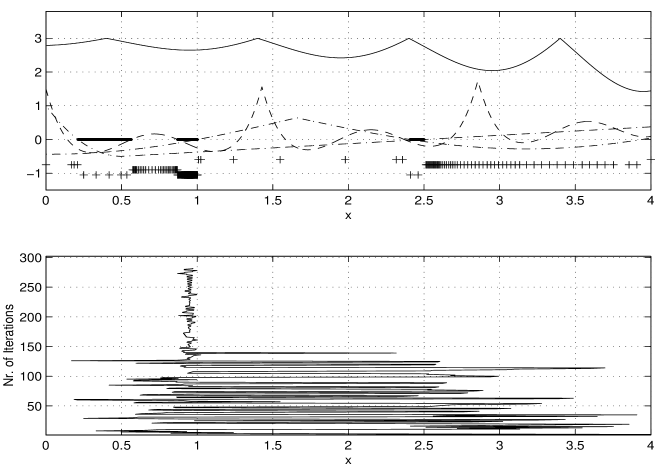
Figure 4: Behaviour of the new method on the non-differentiable problem 9 from [13].

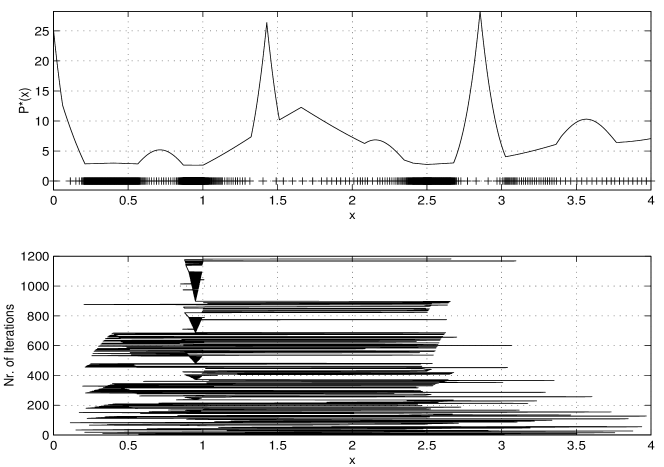
Figure 5: Behaviour of the PEN on the non-differentiable problem $9$ from [13].

The first line (from up to down) of “+” located under the graph of the problem 9 in the upper subplot of Fig. 4 represents the points where the first constraint has not been satisfied (number of iterations equal to 8). Thus, due to the decision rules of the ACIF, the second constraint has not been evaluated at these points. The second line of “+” represents the points where the first constraint has been satisfied but the second constraint has been not (number of iterations equal to 59). In these points both constraints have been evaluated but the objective function has been not. The third line of “+” represents the points where both the first and the second constraints have been satisfied but the third constraint has been not (number of iterations equal to 32). The last line represents the points where all the constraints have been satisfied and, therefore, the objective function has been evaluated (number of evaluations equal to 183). The total number of evaluations is equal to $8+59\times 2+32\times 3+183\times 4=954$. These evaluations have been executed during $8+59+32+183=282$ iterations. The lower subplot in Fig. 4 shows dynamics of the search.

Fig. 5 shows the penalty function corresponding to $P=15$ and dynamics of the search executed by the PEN. The line of “+” located under the graph in the upper subplot of Fig. 5 represents the points where the function (39) has been evaluated. The number of iterations is equal to $1183$ and the number of evaluations is equal to $1183\times 4=4732$.

References

- [1] Archetti F. and F. Schoen (1984), A survey on the global optimization problems: general theory and computational approaches, Annals of Operations Research, 1, 87–110.
- [2] Bertsekas D.P. (1996), Constrained Optimization and Lagrange Multiplier Methods, Athena Scientific, Belmont, MA.
- [3] Bertsekas D.P. (1999), Nonlinear Programming, Second Edition, Athena Scientific, Belmont, MA.
- [4] Bomze I.M., T. Csendes, R. Horst, and P.M. Pardalos (1997) Developments in Global Optimization, Kluwer Academic Publishers, Dordrecht.
- [5] Breiman L. and A. Cutler (1993), A deterministic algorithm for global optimization,Math. Programming, 58, 179–199.
- [6] Brooks S.H. (1958), Discussion of random methods for locating surface maxima, Operation Research, 6, 244–251.
- [7] Calvin J. and A. Žilinskas (1999), On the convergence of the P-algorithm for one-dimensional global optimization of smooth functions, JOTA, 102, 479–495.
- [8] L. G. Casado, I. García, and Y. D. Sergeyev (2000), Interval branch and bound algorithm for finding the First-Zero-Crossing-Point in one-dimensional functions, Reliable Computing, 2, 179–191.
- [9] L. G. Casado, I. García, and Y. D. Sergeyev (2002), Interval algorithms for finding the minimal root in a set of multiextremal non-differentiable one-dimensional functions, SIAM J. on Scientific Computing, 24(2), 359–376.
- [10] P. Daponte, D. Grimaldi, A. Molinaro, and Y. D. Sergeyev (1995), An algorithm for finding the zero crossing of time signals with Lipschitzean derivatives, Measurements, 16, 37–49.
- [11] P. Daponte, D. Grimaldi, A. Molinaro, and Y. D. Sergeyev (1996), Fast detection of the first zero-crossing in a measurement signal set, Measurements, 19, 29–39.
- [12] Evtushenko Yu.G., M.A. Potapov and V.V. Korotkich (1992), Numerical methods for global optimization, Recent Advances in Global Optimization, ed. by C.A. Floudas and P.M. Pardalos, Princeton University Press, Princeton.
- [13] Famularo D., Sergeyev Ya.D., and P. Pugliese (2002), Test Problems for Lipschitz Univariate Global Optimization with Multiextremal Constraints, Stochastic and Global Optimization, eds. G. Dzemyda, V. Saltenis and A. Žilinskas, Kluwer Academic Publishers, Dordrecht, 93-110.
- [14] Floudas C.A. and P.M. Pardalos (1996), State of the Art in Global Optimization, Kluwer Academic Publishers, Dordrecht.
- [15] Hansen P. and B. Jaumard (1995), Lipshitz optimization. In: Horst, R., and Pardalos, P.M. (Eds.). Handbook of Global Optimization, 407-493, Kluwer Academic Publishers, Dordrecht.
- [16] Horst R. and P.M. Pardalos (1995), Handbook of Global Optimization, Kluwer Academic Publishers, Dordrecht.
- [17] Horst R. and H. Tuy (1996), Global Optimization - Deterministic Approaches, Springer–Verlag, Berlin, Third edition.
- [18] Lamar B.W. (1999), A method for converting a class of univariate functions into d.c. functions, J. of Global Optimization, 15, 55–71.
- [19] Locatelli M. and F. Schoen (1995), An adaptive stochastic global optimisation algorithm for one-dimensional functions, Annals of Operations research, 58, 263–278.
- [20] Locatelli M. and F. Schoen (1999), Random Linkage: a family of acceptance/rejection algorithms for global optimisation, Math. Programming, 85, 379–396.
- [21] Lucidi S. (1994), On the role of continuously differentiable exact penalty functions in constrained global optimization, J. of Global Optimization, 5, 49–68.
- [22] MacLagan D., Sturge, T., and W.P. Baritompa (1996), Equivalent Methods for Global Optimization, State of the Art in Global Optimization, eds. C.A. Floudas, P.M. Pardalos, Kluwer Academic Publishers, Dordrecht, 201–212.
- [23] Mladineo R. (1992), Convergence rates of a global optimization algorithm, Math. Programming, 54, 223–232.
- [24] Molinaro A., Sergeyev Ya.D. (2001) An efficient algorithm for the zero-crossing detection in digitized measurement signal, Measurement, 30(3), 187–196.
- [25] Nocedal J. and S.J. Wright (1999), Numerical Optimization (Springer Series in Operations Research), Springer Verlag.
- [26] Pardalos P.M. and J.B. Rosen (1990), Eds., Computational Methods in Global Optimization, Annals of Operations Research, 25.
- [27] Patwardhan A.A., M.N. Karim and R. Shah (1987),Controller tuning by a least-squares method, AIChE J., 33, 1735–1737.
- [28] Pijavskii S.A. (1972), An Algorithm for Finding the Absolute Extremum of a Function, USSR Comput. Math. and Math. Physics, 12, 57–67.
- [29] Pintér J.D. (1996), Global Optimization in Action, Kluwer Academic Publisher, Dordrecht.
- [30] Ralston P.A.S., K.R. Watson, A.A. Patwardhan and P.B. Deshpande (1985), A computer algorithm for optimized control, Industrial and Engineering Chemistry, Product Research and Development, 24, 1132.
- [31] Sergeyev Ya.D. (1998), Global one-dimensional optimization using smooth auxiliary functions, Mathematical Programming, 81, 127-146.
- [32] Sergeyev Ya.D. (1999), On convergence of ”Divide the Best” global optimization algorithms, Optimization, 44, 303–325.
- [33] Sergeyev Ya.D., P. Daponte, D. Grimaldi and A. Molinaro (1999), Two methods for solving optimization problems arising in electronic measurements and electrical engineering, SIAM J. Optimization, 10, 1–21.
- [34] Sergeyev Ya.D. (2000), An Efficient Strategy for Adaptive Partition of N-Dimensional Intervals in the Framework of Diagonal Algorithms, Journal of Optimization Theory and Applications, 107, 145–168.
- [35] Sergeyev Ya.D., Famularo D., and P. Pugliese (2001), Index Branch-and-Bound Algorithm for Lipschitz Univariate Global Optimization with Multiextremal Constraints, J. of Global Optimization, 21, 317–341.
- [36] Sergeyev Ya.D. and D.L. Markin (1995), An algorithm for solving global optimization problems with nonlinear constraints, J. of Global Optimization, 7, 407–419.
- [37] Strongin R.G. (1978), Numerical Methods on Multiextremal Problems, Nauka, Moscow, (In Russian).
- [38] Strongin, R.G. (1984), Numerical methods for multiextremal nonlinear programming problems with nonconvex constraints. In: Demyanov, V.F., and Pallaschke, D. (Eds.) Lecture Notes in Economics and Mathematical Systems 255, 278-282. Proceedings 1984. Springer-Verlag. IIASA, Laxenburg/Austria.
- [39] Strongin R.G. and D.L. Markin (1986), Minimization of multiextremal functions with nonconvex constraints, Cybernetics, 22, 486–493.
- [40] Strongin R.G. and Ya.D. Sergeyev (2000), Global Optimization with Non-Convex Constraints: Sequential and Parallel Algorithms, Kluwer Academic Publishers, Dordrecht.
- [41] Sun X.L. and D. Li (1999), Value-estimation function method for constrained global optimization, JOTA, 102, 385–409.
- [42] Törn A. and A. Žilinskas (1989), Global Optimization, Springer–Verlag, Lecture Notes in Computer Science, 350.
- [43] Wang X. and T.S.Chang (1996), An improved univariate global optimization algorithm with improved linear bounding functions, J. of Global Optimization, 8, 393–411.
- [44] Zhigljavsky A.A. (1991), Theory of Global Random Search, Kluwer Academic Publishers, Dordrecht.