Diagrammatics for $SU(2)$ invariant matrix product states

Abstract

We report on a systematic implementation of $su(2)$ invariance for matrix product states (MPS) with concrete computations cast in a diagrammatic language. As an application we present a variational MPS study of a spin-1/2 quantum chain. For efficient computations we make systematic use of the $su(2)$ symmetry at all steps of the calculations: (i) the matrix space is set up as a direct sum of irreducible representations, (ii) the local matrices with state-valued entries are set up as superposition of $su(2)$ singlet operators, (iii) products of operators are evaluated algebraically by making use of identities for $3j$ and $6j$ symbols. The remaining numerical computations like the diagonalization of the associated transfer matrix and the minimization of the energy expectation value are done in spaces free of symmetry degeneracies. The energy expectation value is a strict upper bound of the true ground-state energy and yields definite conclusions about the accuracy of DMRG results reported in the literature. Furthermore, we present explicit results with accuracy better than $10^{-4}$ for nearest- and next-nearest neighbour spin correlators and for general dimer-dimer correlators in the thermodynamical limit of the spin-$\frac{1}{2}$ Heisenberg chain with frustration.

1 Introduction

We use a systematic implementation of $su(2)$ invariance for matrix-product states (MPS), which parallels [1, 2], and perform a variational $su(2)$-MPS study for the frustrated antiferromagnetic spin-$\frac{1}{2}$ Heisenberg chain.

The class of MPS is of particular importance for the study of quantum spin chains. The MPS appear in different, but closely related ways. Historically, products of matrices with entries from a local Hilbert space first appeared as exact ground-states (matrix-product ground-states, MPG) for Hamiltonians with special local ground-state structure, see [3, 4] and developments [5]-[13]. Second, in the literature on integrable systems, vertex-operators [20]-[22] were introduced for a transfer-matrix like construction of ground-states of lattice systems. Third, the density-matrix renormalization group (DMRG) [14]-[17] algorithms were shown [18, 19] to result in states of MPS type. The MPG, vertex-operators and DMRG are all realizations of MPS. Consequently, this important class of states attracted strong interest in the quantum computation community [23]-[29].

In applications of MPS, details may differ strongly. For instance, in MPG and DMRG realizations the matrix index space is finite dimensional, whereas in the vertex-operator case this space is mostly infinite dimensional. In MPG, the MPS are used as an ansatz for an “exact state” for which a “parental Hamiltonian” is to be found in subsequent investigations. In DMRG, the MPS appear as variational states for the Hamiltonian. In case of the vertex-operator, the full ground-state structure is captured at the expense of infinite-dimensional matrices.

Our investigation is motivated by the need for a computationally most efficient scheme for general $su(2)$ singlet states of MPS type. The local implementation of Lie group invariance has been studied in for instance [33] where $su(2)$ invariant MPG and parental Hamiltonians were investigated, and particularly in the early work [1, 2] where also the variational analysis of $su(2)$ invariant MPS for quantum chains and ladders was introduced. The paper [1] is well-known for the insight that the finite-system DMRG leads to quantum states in MPS form, over which it variationally optimizes. To our knowledge the computational scheme of $su(2)$ invariant MPS with arbitrary matrix space did not attract the attention the papers [1, 2] deserve. Non-Abelian symmetries were implemented in DMRG studies in for instance [30, 31].

Here we use a variational computation scheme very similar to [1, 2] based on $su(2)$ invariant MPS. However, we reduce the necessary constructions to a minimum without taking any reference to DMRG algorithms. Also, we are going to use a diagrammatic representation of some of the key objects and relations occurring in the process of the evaluation of the norm and the energy expectation value of the MPS. We hope, this approach will make the subject as accessible as possible. Our main application will be the study of ground-state energies, spin-spin and dimer-dimer correlations of the (frustrated) antiferromagnetic spin-1/2 Heisenberg chain with nearest- and next-nearest neighbour interactions. For not too strong frustration, this system shows critical behaviour. Still, the variational $su(2)$ invariant MPS give excellent results even for the correlation functions. Probably, and in contrast to the expectation expressed in [2], the approach is applicable even to odd-legged spin-1/2 ladders that are not finitely correlated.

Obviously, and following scientific lore, it is important to use all available symmetries to find invariant blocks of the transfer matrix as low dimensional as possible in order to reduce the computational work involved with the diagonalization procedure. Even more important than the economical treatment of the transfer matrix is the efficient, nonredundant parameterization of the local building elements, i.e. the matrices with entries from the local Hilbert space. It is essential to parameterize these objects with as few parameters as possible to reduce the computational time of the minimization of the energy expectation value.

The paper is organized as follows. In Sect. 2 we present a fairly general derivation of equilibrium states in the form of MPS and shortly summarize the tensor calculus of MPS with emphasis on realizations of symmetries. In Sect. 3 we introduce the $su(2)$ invariant local objects based on Wigner’s $3j$ symbols. Here we also introduce the transfer matrices and evaluate products of operators by making use of identities involving $3j$ and $6j$ symbols. In Sect. 4 we present explicit results from numerical evaluations of the basic formulas derived in the previous section. The results are compared with DMRG data of the literature [32] for the frustrated spin-$\frac{1}{2}$ Heisenberg chain and conclusions about the accuracy of the methods are drawn.

2 Derivation of matrix product states and realization of $SU(2)$ invariance

We are going to study quantum spin systems with local interactions. It is well-known that quantum system in $d$ spatial dimensions can be mapped to classical systems in $d+1$ dimensions. In this way, the ground-state properties of a quantum chain in the thermodynamical limit are encoded by a classical system on an unrestricted 2-dimensional square lattice. Often, for numerical purposes, the quantum chain is mapped onto a kind of Ising model on a square lattice with chequerboard structure, for analytical purposes the mapping of quantum chains onto vertex models on periodic square lattices is more convenient. (The associated classical vertex model has nearest-neighbour couplings even for quantum spin-chains with interactions ranging farther than nearest-neighbours.) Here, the reasoning is based on equilibrium states, but obviously the derivation is more general and covers all steady state systems with local interactions.

After mapping the quantum chain onto a vertex model, the correlation functions of the classical model on the full plane yield the correlations of the quantum chain, as is well-known. It is less well-known, but equally easy to understand that the partition function of a half-plane with arbitrary, but fixed boundary spins yields the coefficients of the ground-state of the quantum chain with respect to the standard basis. The evolution operator associated with a column of the full plane is known as the transfer matrix of the model. The corresponding objects of the half-plane are known as (lattice) vertex operators.

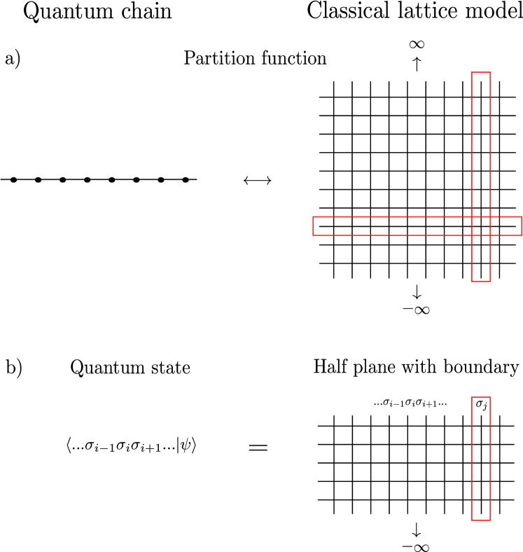
Figure 1: a) Illustration of the relation of quantum spin chains and classical models on square lattices. The rows and columns of the square lattice define the action of the row-to-row and the column-to-column transfer matrix. b) The coordinates $\langle...\sigma_{i-1}\sigma_{i}\sigma_{i+1}...|\psi\rangle$ of the ground-state of the quantum system correspond to the partition functions of the classical model on the half-plane with fixed boundary spins $...\sigma_{i-1}\sigma_{i}\sigma_{i+1}...$. The column of the half-plane with fixed boundary defines the vertex operator.

With view to Fig. 1 these objects carry spin variables on the left, on the right and one spin variable on the top. When considering these objects as matrices where the spin variables on the left play the role of the row index, and the spin variables on right play the role of the column index, vertex operators are matrices with (local) spin state valued entries. The goal of the DMRG procedure may be understood as the computation of the optimal truncation of the infinite dimensional vertex operator to a finite dimensional matrix space. In this section we present the algebraic background for the construction of general $su(2)$ invariant MPS.

We first summarize the basic algebraic constructions needed for our investigation of many-body quantum spin systems. We place particular emphasis on the compatibility with symmetry groups notably Lie groups. Eventually we will be interested in the Lie group $SU(2)$ which is the reason for being specific from the beginning.

We consider the class of matrix-product states

$$|\psi\rangle=\Tr(g_{1}\cdot g_{2}\cdot...\cdot g_{L})$$ (1)

where $g_{i}$ is a square matrix with some auxiliary (index) space $V$ and entries from a local quantum space $V_{i}$ which we take as the $i$th copy of a $su(2)$ spin-$s$ space $\mathbb{C}^{2s+1}$.

$SU(2)$-invariance of $|\psi\rangle$ is guaranteed if for the representation $U_{s}$ of $SU(2)$ in $\mathbb{C}^{2s+1}$ there is a representation $U_{V}$ in $V$ such that $U_{s}$ applied to any element of the matrix $g_{i}$, denoted by $U_{s}g_{i}$, yields a matrix identical to $U_{V}^{-1}\cdot g_{i}\cdot U_{V}$ where dots refer to matrix multiplication. Obviously we obtain with (1)

$$U_{s}\otimes U_{s}\otimes...\otimes U_{s}|\psi\rangle =\Tr(U_{s}g_{1}\cdot U_{s}g_{2}\cdot...\cdot U_{s}g_{L})$$

$$=\Tr(U_{V}^{-1}\cdot g_{1}\cdot U_{V}\cdot U_{V}^{-1}\cdot g_{2}\cdot U_{V}\cdot...\cdot U_{V}^{-1}\cdot g_{L}\cdot U_{V})$$

$$=|\psi\rangle$$ (2)

The local condition for $SU(2)$-invariance can be written as

$$U_{V}\otimes U_{s}\ g\ U_{V}^{-1}=g,$$ (3)

meaning that the object $g$ may be regarded as a tensor of the space $V\otimes\mathbb{C}^{2s+1}\otimes V^{*}$ where $V^{*}$ is the dual space to $V$. (Note that the product $A\cdot B$ of two linear maps $A$ and $B$ of the space $V$ corresponds to the tensor product followed by a contraction of $A$ and $B$ viewed as tensors in $V\otimes V^{*}$.)

For the purpose of imposing discrete lattice symmetries like parity, i.e. invariance with respect to reflections, we adopt a different point of view. Let us consider tensors $G$ from $V\otimes\mathbb{C}^{2s+1}\otimes V$. As a local condition for $SU(2)$-invariance we demand

$$U_{V}\otimes U_{s}\otimes U_{V}\ G=G,$$ (4)

and as a local condition for parity invariance we demand – as a sufficient condition – that $G$ be symmetric with respect to exchange of “the first and the third index” when written in a canonical basis.

The relation between $g$ and $G$ is realized by a $SU(2)$-invariant tensor $S$ from $V\otimes V$ (and by the invariant dual tensor $S^{*}$ from $V^{*}\otimes V^{*}$). Concrete candidates for $S$ (and $S^{*}$) will be given shortly.

The tensor $S$ can equivalently be understood as a linear map from $V^{*}$ to $V$ as the multiplication of an arbitrary element $\tilde{v}$ of $V^{*}$ with $S$ yields an object in $V^{*}\otimes V\otimes V$, the subsequent contraction over the first and second space yields an element $v$ of $V$. Denoting $S(\tilde{v}):=v$ we establish $S$ as a map $V^{*}\to V$. The $SU(2)$-invariance of $S$ as a tensor in $V\otimes V$ is written as $U_{V}\otimes U_{V}\ S=S$ from which we find

$$S(\tilde{v}U_{V}^{-1})=U_{V}v=U_{V}S(\tilde{v}).$$ (5)

The object $G$ is obtained by action of $S$ on the third space of $g$

$$G={\rm id}\otimes{\rm id}\otimes S\ g$$ (6)

which takes (3) into (4) thanks to (5).

Conversely, we establish $S^{*}$ as a linear map $V\to V^{*}$ with $SU(2)$-invariance $S^{*}(U_{V}v)=S^{*}(v)U_{V}^{-1}$ and for the concrete realizations of $S$ and $S^{*}$ we find $S\cdot S^{*}=(-1)^{2j}$ and $S^{*}\cdot S=(-1)^{2j}$ in spin-$j$ subspaces. Hence, $S$ and $S^{*}$ are invertible and $g={\rm id}\otimes{\rm id}\otimes S^{-1}\ G$.

Finally, we have to give explicit constructions for $S$ (and $S^{*}$) as $SU(2)$-invariant states in $V\otimes V$. This is the only place where we make explicit use of the fact that our Lie symmetry group is $SU(2)$. We take the space $V$ as a direct sum of some irreducible spin-$j$ representations where $j=0,\frac{1}{2},1,\frac{3}{2},2,...$ . Each $j$ may appear an arbitrary number of times, in which case we label the different orthogonal mupltiplets by an integer $i$. The space $V$ is spanned by orthogonal states $|(j,i),m\rangle$ where the magnetic quantum number $m$ varies from $-j$ to $+j$ in integer steps. $SU(2)$ singlet states in $V\otimes V$ and $V^{*}\otimes V^{*}$ are given by

$$S:=\sum_{j,i}\sum_{m=-j}^{j}(-1)^{j-m}|(j,i),m\rangle\otimes|(j,i),-m\rangle,$$

$$S^{*}:=\sum_{j,i}\sum_{m=-j}^{j}(-1)^{j-m}\langle(j,i),m|\otimes\langle(j,i),-m|.$$ (7)

where $S^{*}$ is related to $S$ by replacing the ket-states by the dual bra-states.

Applying our above formulated definitions we find for $\tilde{v}=\langle(j,i),m|$ that $S(\tilde{v})=(-1)^{j-m}|(j,i),-m\rangle$. Conversely, for $v=|(j,i),m\rangle$ we have $S^{*}(v)=(-1)^{j-m}\langle(j,i),-m|$. Hence, the successive action of $S$ and $S^{*}$ yields $(-1)^{2j}\,{\rm id}$.

3 Basic representation theoretical settings: $3j$ and $6j$ symbols

Having spelled out the fundamental objects appearing as factors in $SU(2)$-invariant matrix-product states, the concrete calculations are straightforward. We want to use $SU(2)$ singlets $G$ in $V\otimes\mathbb{C}^{2s+1}\otimes V$. Having already allowed for reducible representations in $V$, we like to stress that for our applications we must deal with $V$ as direct sum of more than one irreducible representation. This is so as for the most interesting case of $s=\frac{1}{2}$ no singlet $G$ exists if $V$ is identical to just one spin-$j$ multiplet. There is no half-integer spin in the tensor product decomposition of two spin-$j$’s!

Let us consider in $V\otimes\mathbb{C}^{2s+1}\otimes V$ any spin multiplet $(j_{1},i_{1})$ from the first factor space, the (only) spin multiplet $j_{2}\,(=s)$ of the second space, and again any spin multiplet $(j_{3},i_{3})$ from the third factor space. Disregarding scalar factors, there is at most one way of coupling these multiplets to a singlet state. The coupling coefficients are known as $3j$ symbols and the desired singlet is

$$|(j_{1},i_{1}),j_{2},(j_{3},i_{3})\rangle:=$$

$$\sum_{m_{1},m_{2},m_{3}}\left(\hbox{\begin{tabular}[]{ccc}$j_{1}$&$j_{2}$&$j_{3}$\\ $m_{1}$&$m_{2}$&$m_{3}$\end{tabular}}\right)|(j_{1},i_{1}),m_{1}\rangle\otimes|j_{2},m_{2}\rangle\otimes|(j_{3},i_{3}),m_{3}\rangle.$$ (10)

Further below we will be using a graphical language for constructions and actual calculations. For instance, the singlet (10) and its dual are depicted by three straight lines carrying arrows, see Fig. 2.

Figure 2: Introduction of the graphical notation for singlets appearing in product spaces. Three leg (vertex) symbols for $|(j_{1},i_{1}),j_{2},(j_{3},i_{3})\rangle$ and $\langle(j_{1},i_{1}),j_{2},(j_{3},i_{3})|$ appearing in products of three irreducible representations. Two leg (edge) symbols for the singlets $S$ resp. $S^{*}$ in $V\times V$ resp. $V^{*}\times V^{*}$, and arcs for singlets in $V\times V^{*}$ for the same spin $j$.

The coupling coefficients of the singlets shown in Fig. 2 are given in Fig. 3. More precisely, the objects shown Fig. 2 are obtained by multiplying the objects in Fig. 3 by states $|(j,i),m\rangle$ (or the dual) and summing over all magnetic quantum numbers $m$.

Figure 3: Graphical notation for key arithmetic objects like Kronecker symbol and $3j$ symbol.

The singlet $G$ can be written as superposition of these elementary singlets

$$G=\sum_{(j_{1},i_{1}),(j_{3},i_{3})}A^{j_{1},j_{3}}_{i_{1},i_{3}}|(j_{1},i_{1}),j_{2},(j_{3},i_{3})\rangle$$ (11)

with suitable coefficients $A^{j_{1},j_{3}}_{i_{1},i_{3}}$. Note that $j_{2}$ has been suppressed as index-like argument of $A$ as $j_{2}$ is always identical to $\frac{1}{2}$ and unique (for this reason no $i_{2}$ has been introduced above). Due to the symmetry of $3j$ symbols with respect to exchange of two columns

$$\left(\hbox{\begin{tabular}[]{ccc}$j_{3}$&$j_{2}$&$j_{1}$\\ $m_{3}$&$m_{2}$&$m_{1}$\end{tabular}}\right)=(-1)^{j_{1}+j_{2}+j_{3}}\left(\hbox{\begin{tabular}[]{ccc}$j_{1}$&$j_{2}$&$j_{3}$\\ $m_{1}$&$m_{2}$&$m_{3}$\end{tabular}}\right)$$ (12)

we conclude that

$$A^{j_{3},j_{1}}_{i_{3},i_{1}}=(-1)^{j_{1}+j_{2}+j_{3}}A^{j_{1},j_{3}}_{i_{1},i_{3}}.$$ (13)

is a sufficient condition for parity invariance. Note that $j_{1}+j_{2}+j_{3}$ is always integer.

Also note that only few combinations ${j_{1}},{j_{2}},{j_{3}}$ need to be considered: if the triangle condition $|j_{1}-j_{2}|\leq j_{3}\leq|j_{1}+j_{2}|$ or any condition obtained by permutations of the indices is violated, the three multiplets can not couple to a singlet. Since $j_{2}=\frac{1}{2}$, we are left with the combinations $\{j_{1},j_{3}\}=\{0,\frac{1}{2}\},\{\frac{1}{2},1\},\{1,\frac{3}{2}\},...$. This is a natural result, since $j_{1}$ and $j_{2}=\frac{1}{2}$ only couple to $j_{1}\pm\frac{1}{2}$. Let us denote by $n_{j}$ the number of spin-$j$ multiplets. By use of the symmetry (13) we may reduce all possible coefficients $A$ to a set of $n_{j}\times n_{j+\nicefrac{{1}}{{2}}}$ matrices $A^{j,j+\nicefrac{{1}}{{2}}}$ with matrix elements

$$\Big{(}A^{j,j+\nicefrac{{1}}{{2}}}\Big{)}_{i_{l},i_{r}}:=A^{j,j+\nicefrac{{1}}{{2}}}_{i_{l},i_{r}}.$$ (14)

3.1 Norm and transfer matrix

Next, we want to calculate the norm $\langle\psi|\psi\rangle$ and the expectation value of the Hamiltonian $\langle\psi|H|\psi\rangle$ in the thermodynamic limit. The computation leads to

$$\langle\psi|\psi\rangle=\Tr(g_{1}^{+}g_{1}\cdot g_{2}^{+}g_{2}\cdot...\cdot g_{L}^{+}g_{L}),$$ (15)

where $g^{+}$ $\in V^{*}\otimes(\mathbb{C}^{2s+1})^{*}\otimes V$ is the dual of $g$ $\in V\otimes\mathbb{C}^{2s+1}\otimes V^{*}$ and the contraction over the second space is implicitly understood in $g^{+}g$. Hence $T:=g^{+}g$ is a linear map $V\otimes V^{*}\to V\otimes V^{*}$. For the computation of the norm we employ the transfer matrix trick yielding for the r.h.s. of (15)

$$\langle\psi|\psi\rangle=\Tr(\underbrace{T\cdot...\cdot T}_{L\ \mbox{times}})=\sum_{\Lambda}\Lambda^{L},$$ (16)

where the sum is over all eigenvalues $\Lambda$ of $T$. Obviously, in the thermodynamic limit only the largest eigenvalue(s) contribute.

The computation of the leading eigenvalue is facilitated by the singlet nature of the leading eigenstate. There are not many independent singlet states in $V\otimes V^{*}$. A $(j,i)$ multiplet in $V$ and a $(\tilde{j},\tilde{i})$ multiplet in $V^{*}$ couple to a singlet iff $j=\tilde{j}$ (with arbitrary $i$ and $\tilde{i}$). The (normalized) singlet is given by

$$\sigma(j;i,\tilde{i}):=\frac{1}{\sqrt{2j+1}}\sum_{m=-j}^{j}|j,i,m\rangle\otimes\langle j,\tilde{i},m|.$$ (17)

Graphicially, this singlet is depicted by a link carrying an arrow pointing from the $V^{*}$ to the $V$ space.

The action of the transfer matrix $T$ onto a singlet $\sigma(j;i,\tilde{i})$ produces similar singlets where $j$ is changed by $\pm\frac{1}{2}$. The $\sigma(j_{l};i_{l},\tilde{i}_{l})-\sigma(j_{r};i_{r},\tilde{i}_{r})$ matrix element of $T$ is

$$\langle j_{l};i_{l},\tilde{i}_{l}|T|j_{r};i_{r},\tilde{i}_{r}\rangle=\frac{1}{\sqrt{(2j_{l}+1)(2j_{r}+1)}}A^{j_{l},j_{r}}_{i_{l},i_{r}}\Big{(}A^{j_{l},j_{r}}_{\tilde{i}_{l},\tilde{i}_{r}}\Big{)}^{*},$$ (18)

where $j_{l}=j_{r}\pm\frac{1}{2}$. (Expression (18) is the analogue of eq. (6) in [2], but here we do not impose condition (10) of [2].) The matrix $T$ has a simple block structure with zero diagonal blocks and non-zero secondary diagonal blocks. From (13) we conclude that the matrix is symmetric. The defining blocks are

$$\langle j;i_{l},\tilde{i}_{l}|T|j+\nicefrac{{1}}{{2}};i_{r},\tilde{i}_{r}\rangle=\frac{1}{\sqrt{(2j+1)(2j+2)}}A^{j,j+\nicefrac{{1}}{{2}}}_{i_{l},i_{r}}\Big{(}{A^{j,j+\nicefrac{{1}}{{2}}}_{\tilde{i}_{l},\tilde{i}_{r}}}\Big{)}^{*}.$$ (19)

In expression (18) the coefficients $A$ and the complex conjugate $A^{*}$ derive from the explicit appearance in (11) and the prefactor is obtained from the identity of $3j$ symbols (if $j_{1}$ is found in the product of $j_{2}$ and $j_{3}$)

$$\sum_{m_{2},m_{3}}\left(\hbox{\begin{tabular}[]{ccc}$j_{1}^{\prime}$&$j_{2}$&$j_{3}$\\ $m_{1}^{\prime}$&$m_{2}$&$m_{3}$\end{tabular}}\right)\left(\hbox{\begin{tabular}[]{ccc}$j_{1}$&$j_{2}$&$j_{3}$\\ $m_{1}$&$m_{2}$&$m_{3}$\end{tabular}}\right)=\frac{1}{2j_{1}+1}\delta_{j_{1},j_{1}^{\prime}}\delta_{m_{1},m_{1}^{\prime}},$$ (20)

illustrated in Fig. 4.

Figure 4: Illustration of identity (20): The summation over two internal magnetic quantum numbers leads to an “arc”-singlet.

The computation of the matrix elements of $T$ is graphically presented in Fig. 5.

Figure 5: Depiction of the transfer matrix $T$ in terms of local vertices and the action onto singlet states.

For a given space $V$ with a certain number of spin-0, $\frac{1}{2}$, 1, $\frac{3}{2}$ … multiplets and a certain set of parameters $A(j_{l},i_{l};j_{r},i_{r})$, the transfer matrix has to be diagonalized in the singlet space. The total number of non-zero coefficients $A(j_{l},i_{l};j_{r},i_{r})$ is $\sum_{j}n_{j}n_{j+\nicefrac{{1}}{{2}}}$ (with sum over $j=0,\frac{1}{2},1,\frac{3}{2},...$ and $n_{j}$ denoting the number of spin-$j$ multiplets). The total dimension of $V\otimes V^{*}$ is $\big{(}\sum_{j}n_{j}(2j+1)\big{)}^{2}$, but the singlet subspace is much lower dimensional: $\sum_{j}n_{j}^{2}$. Due to the still high dimensionality, the diagonalisation in the singlet space has to be done numerically. The eigenvalues come in pairs $\pm\Lambda$. The two largest eigenvalues and the corresponding eigenstates determine the physics in the thermodynamic limit.

3.2 Nearest-neighbour couplings

We are interested in the spin-$\frac{1}{2}$ Heisenberg chain with nearest-neighbour interaction with Hamiltonian

$$H=\sum_{l=1}^{L}\vec{S}_{l}\vec{S}_{l+1}.$$ (21)

The local Hamiltonian is $h_{l,l+1}=\vec{S}_{l}\vec{S}_{l+1}=1/4-P^{nn}_{0}$ where $P^{nn}_{0}$ is the projector onto the nearest-neighbour singlet space. We want to determine the matrix-product state with minimal expectation value of the total Hamiltonian $H=\sum_{l}h_{l}$. Due to translational invariance this is achieved by minimizing the expectation value of a single local interaction. In analogy to (16) we obtain

$$\langle\psi|P^{nn}_{0}|\psi\rangle=\Tr(\tilde{T}\underbrace{T\cdot...\cdot T}_{L-2\ \mbox{times}})=\Lambda_{0}^{L-2}\langle 0|T_{2}|0\rangle,$$ (22)

where we assumed $P^{nn}_{0}$ to act on sites 1 and 2. $T_{2}$ is a modified transfer matrix acting in $V\otimes V^{*}$, $|0\rangle$ is the (normalized) leading eigenstate of the transfer matrix $T$ and we kept the only term dominating in the thermodynamical limit. Hence

$$\frac{\langle\psi|P^{nn}_{0}|\psi\rangle}{\langle\psi|\psi\rangle}=\Lambda_{0}^{-2}\langle 0|T_{2}|0\rangle.$$ (23)

Figure 6: Depiction of the modified matrix $T_{2}$ in terms of local vertices.

Figure 7: The summation over two internal magnetic quantum numbers leads to an “edge”-singlet.

The computation of the matrix elements of $T_{2}$ is described graphically in Figs. 6 and 7. In contrast to the transfer matrix $T$ the modified matrix $T_{2}$ is block diagonal with $\sigma(j;i_{l},\tilde{i}_{l})-\sigma(j;i_{r},\tilde{i}_{r})$ matrix element

$$\langle j;i_{l},\tilde{i}_{l}|T_{2}|j;i_{r},\tilde{i}_{r}\rangle=\frac{1}{(2j+1)^{2}}B^{j,j}_{i_{l},i_{r}}\Big{(}B^{j,j}_{\tilde{i}_{l},\tilde{i}_{r}}\Big{)}^{*}.$$ (24)

The matrices $B$ are given by

$$B^{j,j}=\sum_{j_{1}}(-1)^{\nicefrac{{1}}{{2}}+j+j_{1}}A^{j,j_{1}}A^{j_{1},j},$$ (25)

where only the values $j_{1}=j\pm\frac{1}{2}$ lead to non-zero terms. (Equations (24,25) are the analogue of eq. (26) in [2].) Using this and the (sufficient) condition (13) for parity invariance we find

$$B^{j,j}=\Big{[}A^{j-\nicefrac{{1}}{{2}},j}\Big{]}^{T}A^{j-\nicefrac{{1}}{{2}},j}+A^{j,j+\nicefrac{{1}}{{2}}}\Big{[}A^{j,j+\nicefrac{{1}}{{2}}}\Big{]}^{T}.$$ (26)

3.3 Next-Nearest-neighbour couplings

The next-nearest neighbour interactions are manageable, too. In the thermodynamical limit we find

$$\frac{\langle\psi|P^{nnn}_{0}|\psi\rangle}{\langle\psi|\psi\rangle}=\Lambda_{0}^{-3}\langle 0|T_{3}|0\rangle.$$ (27)

Figure 8: Depiction of the modified matrix $T_{3}$ in terms of local vertices.

Figure 9: The summation over three internal magnetic quantum numbers leads to a $6j$ symbol times an elementary vertex.

The computation of the matrix elements of $T_{3}$ is described graphically in Fig. 8 and Fig. 9. In contrast to the modified transfer matrix $T_{2}$, but like $T$, the matrix $T_{3}$ has zero diagonal blocks and non-zero secondary diagonal blocks. The $\sigma(j_{l};i_{l},\tilde{i}_{l})-\sigma(j_{r};i_{r},\tilde{i}_{r})$ matrix element of $T_{3}$ is

$$\langle j_{l};i_{l},\tilde{i}_{l}|T_{3}|j_{r};i_{r},\tilde{i}_{r}\rangle=\frac{1}{\sqrt{(2j_{l}+1)(2j_{r}+1)}}C^{j,j+\nicefrac{{1}}{{2}}}_{i_{l},i_{r}}\Big{(}{C^{j,j+\nicefrac{{1}}{{2}}}_{\tilde{i}_{l},\tilde{i}_{r}}}\Big{)}^{*}.$$ (28)

where $j_{l}=j_{r}\pm\frac{1}{2}$ and $C^{j_{l},j_{r}}$ is given by

$$C^{j_{l},j_{r}}=\sum_{j_{1},j_{3}}(-1)^{\nicefrac{{1}}{{2}}+j_{1}+j_{3}}\left\{\hbox{\begin{tabular}[]{ccc}$j_{l}$&$\nicefrac{{1}}{{2}}$&$j_{r}$\\ $j_{3}$&$\nicefrac{{1}}{{2}}$&$j_{1}$\end{tabular}}\right\}A^{j_{l},j_{1}}A^{j_{1},j_{3}}A^{j_{3},j_{r}}.$$ (29)

(There is no analogue to eqs. (28,29) in [1, 2].) Only three combinations of $j_{1},j_{3}$ yield non-vanishing contributions. For $j_{r}=j_{l}+1/2$ only $(j_{1},j_{3})=$ $(j_{l}-1/2,j_{l})$, $(j_{l}+1/2,j_{l})$, $(j_{l}+1/2,j_{l}+1)$ are relevant. From this and the (sufficient) condition (13) for parity invariance we find

$$C^{j,j+\nicefrac{{1}}{{2}}} =\left\{\hbox{\begin{tabular}[]{ccc}$j$&$\nicefrac{{1}}{{2}}$&$j+\nicefrac{{1}}{{2}}$\\ $j$&$\nicefrac{{1}}{{2}}$&$j-\nicefrac{{1}}{{2}}$\end{tabular}}\right\}\Big{(}A^{j-\nicefrac{{1}}{{2}},j}\Big{)}^{T}A^{j-\nicefrac{{1}}{{2}},j}A^{j,j+\nicefrac{{1}}{{2}}}$$ (32)

$$+\left\{\hbox{\begin{tabular}[]{ccc}$j$&$\nicefrac{{1}}{{2}}$&$j+\nicefrac{{1}}{{2}}$\\ $j$&$\nicefrac{{1}}{{2}}$&$j+\nicefrac{{1}}{{2}}$\end{tabular}}\right\}A^{j,j+\nicefrac{{1}}{{2}}}\Big{(}A^{j,j+\nicefrac{{1}}{{2}}}\Big{)}^{T}A^{j,j+\nicefrac{{1}}{{2}}}$$ (35)

$$+\left\{\hbox{\begin{tabular}[]{ccc}$j$&$\nicefrac{{1}}{{2}}$&$j+\nicefrac{{1}}{{2}}$\\ $j+1$&$\nicefrac{{1}}{{2}}$&$j+\nicefrac{{1}}{{2}}$\end{tabular}}\right\}A^{j,j+\nicefrac{{1}}{{2}}}A^{j+\nicefrac{{1}}{{2}},j+1}\Big{(}A^{j+\nicefrac{{1}}{{2}},j+1}\Big{)}^{T},$$ (38)

where the $6j$ symbols evaluate to

$$\left\{\hbox{\begin{tabular}[]{ccc}$j$&$\nicefrac{{1}}{{2}}$&$j+\nicefrac{{1}}{{2}}$\\ $j$&$\nicefrac{{1}}{{2}}$&$j-\nicefrac{{1}}{{2}}$\end{tabular}}\right\}=\frac{(-1)^{2j+1}}{2j+1},$$ (41)

$$\left\{\hbox{\begin{tabular}[]{ccc}$j$&$\nicefrac{{1}}{{2}}$&$j+\nicefrac{{1}}{{2}}$\\ $j$&$\nicefrac{{1}}{{2}}$&$j+\nicefrac{{1}}{{2}}$\end{tabular}}\right\}=\frac{(-1)^{2j+1}}{(2j+1)(2j+2)},$$ (44)

$$\left\{\hbox{\begin{tabular}[]{ccc}$j$&$\nicefrac{{1}}{{2}}$&$j+\nicefrac{{1}}{{2}}$\\ $j+1$&$\nicefrac{{1}}{{2}}$&$j+\nicefrac{{1}}{{2}}$\end{tabular}}\right\}=\frac{(-1)^{2j}}{2j+2},$$ (47)

with an exception for $j=0$ where the first listed $6j$ symbol has to be taken as 0.

4 Results

For the nearest-neighbour spin-$\frac{1}{2}$ Heisenberg chain we found that already a few low-dimensional multiplets in the matrix space $V$ yield excellent results, e.g. the ground-state energy differs from the exact result $e_{0}=1/4-\ln 2$ by about $5\cdot 10^{-5}$ and dimer correlations are off the exact results by about $10^{-4}$. This is achieved with $n_{0}=4$, $n_{\nicefrac{{1}}{{2}}}=4$, $n_{1}=3$, $n_{\nicefrac{{3}}{{2}}}=2$, $n_{2}=1$ ($n_{s}$=0 for $s>2$). Note that the attempt to include higher spin multiplets at the expense of reducing the low-spin multiplets is not successful as for instance $n_{s}=1$ for all $s$ leads to the simple dimer (Majumdar-Ghosh) state.

The minimization of the energy expectation value yields the following list of coefficients

$$A^{0,\nicefrac{{1}}{{2}}} =\left[\begin{array}[]{cccc}1.0&0&0&0\\ \vskip 6.0pt plus 2.0pt minus 2.0pt\cr 0&-0.283412&0&0\\ \vskip 6.0pt plus 2.0pt minus 2.0pt\cr 0&0&0.183208&0\\ \vskip 6.0pt plus 2.0pt minus 2.0pt\cr 0&0&0&0.679798\end{array}\right],\quad$$ (52)

$$A^{\nicefrac{{1}}{{2}},1} =\left[\begin{array}[]{ccc}0.737765&0&0\\ \vskip 6.0pt plus 2.0pt minus 2.0pt\cr 0.257549&-0.860519&0\\ \vskip 6.0pt plus 2.0pt minus 2.0pt\cr 0.610288&-0.093768&0.050733\\ \vskip 6.0pt plus 2.0pt minus 2.0pt\cr 0.191246&-0.631258&0.181757\end{array}\right]$$ (57)

$$A^{1,\nicefrac{{3}}{{2}}} =\left[\begin{array}[]{cc}0.510676&0\\ \vskip 6.0pt plus 2.0pt minus 2.0pt\cr-0.5075510&0.714082\\ \vskip 6.0pt plus 2.0pt minus 2.0pt\cr-0.292858&0.712182\end{array}\right],\qquad A^{\nicefrac{{3}}{{2}},2}=\left[\begin{array}[]{c}0.265736\\ \vskip 6.0pt plus 2.0pt minus 2.0pt\cr-0.607939\end{array}\right]$$ (63)

and a value of the ground-state energy which compares well with the exact value [34]

$$e_{0}^{\rm num}=-0.443\ 092\ 175...,\qquad e_{0}^{\rm exact}=-0.443\ 147\ 180...$$ (64)

Note that $A^{0,\nicefrac{{1}}{{2}}}$ is strictly diagonal, and the other matrices have strictly zero entries above the diagonal due to a “gauge” freedom. The MPS is invariant under a transformation $A^{j_{l},j_{r}}\to{\cal{O}}_{j_{l}}^{-1}A^{j_{l},j_{r}}{\cal{O}}_{j_{r}}$ where ${\cal{O}}_{j}$ are arbitrary orthogonal $n_{j}\times n_{j}$-matrices. Also note that the entries of the matrices are strictly real.

Next we give numerical results for the dimer-dimer correlation function

$$\tilde{D}_{n}:=\langle(\vec{S}_{1}\cdot\vec{S}_{2})(\vec{S}_{n+1}\cdot\vec{S}_{n+2})\rangle.$$ (65)

For $n\to\infty$ this converges to $e_{0}^{2}$, hence it is more instructive to study the connected dimer correlations

$$D_{n}:=\tilde{D}_{n}-\tilde{D}_{\infty}.$$ (66)

For $n=$ 2, 3, 4 the values are known exactly [35] which we use for comparison with our MPS calculations

$$D_{2}^{\rm num} =+0.060\ 639...,\qquad D_{2}^{\rm exact}=+0.060\ 824...,$$

$$D_{3}^{\rm num} =-0.027\ 838..., D_{3}^{\rm exact}=-0.027\ 737...,$$ (67)

$$D_{4}^{\rm num} =+0.018\ 986..., D_{4}^{\rm exact}=+0.018\ 928....$$

We expect that the absolute numerical accuracy is similar also for larger distances $n$ of the local dimer operators. These results are plotted in Fig. 10 as $(-1)^{n}D_{n}$ versus $n$. Note that all $(-1)^{n}D_{n}$ are positive which implies a sublattice structure with sign alternation of the correlations. There is no long-range order for the spin-$\frac{1}{2}$ Heisenberg chain with nearest-neighbour interactions.

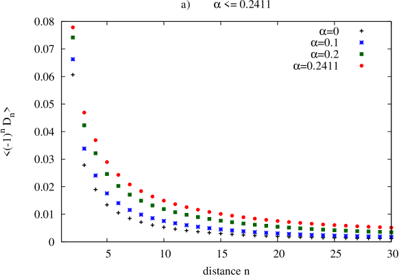
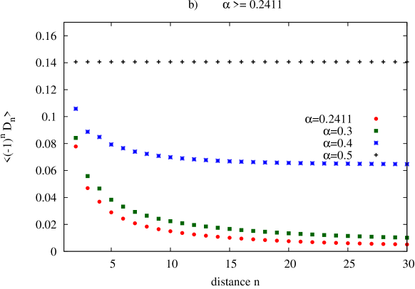
Figure 10: Dimer-dimer correlations of the spin-$\frac{1}{2}$ Heisenberg chain with frustration parameter $\alpha$: Linear plots of $(-1)^{n}D_{n}$ for a) $\alpha=0,0.1,0.2,0.2411$ and b) $\alpha=0.2411,0.3,0.4,0.5$. Note the long-range order in plot b) for $\alpha>0.2411$.

Next we are interested in the frustrated spin-$\frac{1}{2}$ Heisenberg chain with Hamiltonian

$$H=\sum_{l=1}^{L}\left(\vec{S}_{l}\vec{S}_{l+1}+\alpha\vec{S}_{l}\vec{S}_{l+2}\right).$$ (68)

The system shows algebraically decaying dimer-dimer correlations for $\alpha\leq 0.2411...$, see Fig. 11, and long-range dimer order for $\alpha>0.2411...$, see Fig. 10 b). The critical value $\alpha_{c}=0.2411$ was established in [36, 37]. The dimer-dimer correlations are fitted well by algebraic curves for all $\alpha\leq 0.2411..$ with $\alpha$-dependent exponent. From field theoretical considerations the exponent is expected to be identical to 1. We attribute the deviations to logarithmic corrections for $\alpha<0.2411..$ which apparently vanish at $\alpha_{c}$.

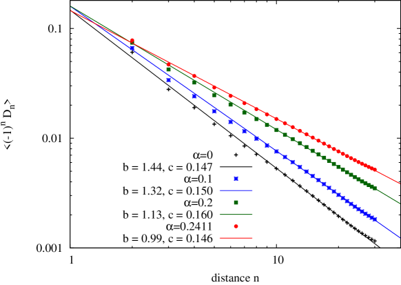
Figure 11: Dimer-dimer correlations of the spin-$\frac{1}{2}$ Heisenberg chain with frustration parameter $\alpha\leq 0.2411$: Double log plot of $(-1)^{n}D_{n}$ versus distance $n$ and algebraic lines $c/n^{b}$ from fits to the data for $n$ in the range $[10,25]$.

As an illustration of spin-spin-correlation functions we present results for the nearest- and next-nearest-neighbour cases in table 1. For $\alpha=0$ the exact values are known [34] $C_{2}^{\rm exact}=e_{0}^{\rm exact}$, see (64), and [35] $C_{3}^{\rm exact}=0.182\ 039...$. Even for $C_{3}$ our numerical value deviates from the exact value less than $10^{-4}$. Due to the variational nature of our calculations the expectation values of the energy are strict upper bounds for the ground-state energy. Note that for cases $\alpha=0.1,0.2411,0.3,0.4$ our results are lower than those given in [32] with small differences ranging from $10^{-4}$ to $10^{-3}$. Hence, the deviation of these DMRG results from the true ground-state energy must be of the same order or even larger. In DMRG calculations there are two sources of errors: (i) truncation of the Hilbert space and (ii) finite-size effects due to the finite length of the considered chains. In our approach we deal with the strictly infinitely long chain.

$\alpha$	0.0	0.1	0.2	$\alpha_{c}$	0.3	0.4	0.5
$C_{2}$	-0.443092	-0.442655	-0.440916	-0.439574	-0.436475	-0.420659	-0.375000
$C_{3}$	0.181942	0.173570	0.162233	0.156176	0.144794	0.100870	0.0
$e_{0}$	-0.443092	-0.425298	-0.408469	-0.401920	-0.393037	-0.380311	-0.375000

Table 1: Numerical values for the correlations $C_{n}:=\langle\vec{S}_{1}\vec{S}_{n+1}\rangle$ for $n=1,2$ and various values of the frustration parameter $\alpha$. The ground-state energy $e_{0}=C_{1}+\alpha C_{2}$ is given in the last row.

The numerical computations of the data presented in this section were done by use of Maple 13 on a laptop computer. The total computation for the seven cases of the frustration parameter took about 1 hour.

A more complete study of the correlation functions and of the physics of frustrated systems with $\alpha>0.5$ will be presented elsewhere. Here we like to note that for $\alpha>0.5$ the matrices replacing (63) will contain intrinsically complex numbers.

5 Conclusion

We showed how to employ systematically $su(2)$ invariance for matrix product states and how to carry out the variational computation of the ground state energy in a numerically most efficient manner. The algebraic computations for the $su(2)$-invariant bulding blocks were put in diagrammatic formulation. As an example we used the (frustrated) spin-$\frac{1}{2}$ Heisenberg chain with nearest- and next-nearest neighbour interaction. Our algebraic constructions led to the main results (18) for the transfer matrix, and (24,25) and (28,29) for the modified transfer matrices, where the coefficient matrix has to satisfy the relation (13) for parity invariance.

Our calculations are very similar to those of [1, 2] who applied the method to gapped spin-1 chains and spin ladders. The variational MPS calculations for the spin-$\frac{1}{2}$ Heisenberg chain are demanding on their own: the model shows algebraically decaying correlation functions and it is by no means clear if signatures of this decay can already be seen in variational MPS calculations with only few multiplets in the matrix space. Also, in contrast to [1, 2], the matrix space we had to deal with consists of all integer and half-odd integer spin multiplets. In our concrete calculation we used a matrix space composed of 4 singlets, 4 doublets, 3 triplets, 2 quadruplets, and 1 quintuplets. We managed to calculate the ground-state energy within a precision better than $10^{-4}$. Also, the correlation functions were computed within an accuracy of the order $10^{-4}$ and allowed for the identification of the scaling dimension in the case of critical frustration ($\alpha=0.2411$).

The actual numerical calculations like matrix diagonalizations were reduced by the algebraic $su(2)$ implementation from a 1156-dimensional to a 46-dimensional space. The systematic inclusion of more and higher spin multiplets is obvious. Generalizations of these calculations are straight forward, e.g. to spin-$S$ Heisenberg chains with competing interactions. We are convinced that a systematic application of symmetries to the MPS analysis of quantum spin chains will provide high quality data with only small truncation errors.

Acknowledgments.

The authors would like to thank F. Göhmann, M. Karbach and J. Sirker for valuable discussions, and J. Dukelsky and A. Schadschneider for relevant information on related work. The authors gratefully acknowledge support by Deutsche Forschungsgemeinschaft under project Renormierungsgruppe KL 645/6-1.

References

References

- [1] J. Dukelsky, M. A. Martin Delgado, T. Nishino and G. Sierra, Equivalence of the Variational Matrix Product Method and the Density Matrix Renormalization Group applied to Spin Chains, Europhys. Lett. 43 (1998) 457.
- [2] J. M. Roman, G. Sierra, J. Dukelsky and M. A. Martin-Delgado, The Matrix Product Approach to Quantum Spin Ladders., J. Phys. A: Math. Gen. 31 (1998) 9729.
- [3] I. Affleck, T. Kennedy, E. H. Lieb and H. Tasaki, Phys. Rev. Lett. 59,799 (1987).
- [4] I. Affleck, T. Kennedy, E. H. Lieb and H. Tasaki, Comm. Math. Phys. 115, 477 (1988).
- [5] M. Fannes, B. Nachtergaele and R. F. Werner, Exact antiferromagnetic ground states of quantum spin chains, Europhys. Lett. 10, 633 (1989).
- [6] M. Fannes, B. Nachtergaele and R. F. Werner, Finitely correlated states on quantum spin chains, Comm. Math. Phys. 144, 443 (1992).
- [7] A. Klümper, A. Schadschneider, J. Zittartz: Equivalence and solution of anisotropic spin-1 models and generalized - fermion models in one dimension J. Phys. A 24, L955-L959 (1991)
- [8] A. Klümper, A. Schadschneider, J. Zittartz: Groundstate properties of a generalized VBS-model Z. Phys. B87, 281-287 (1992)
- [9] A. Klümper, A. Schadschneider, J. Zittartz: Matrix-product-groundstates for one-dimensional spin-1 quantum antiferromagnets Europhys. Lett. 24, 293 (1993)
- [10] C. Lange, A. Klümper, J. Zittartz: Exact groundstates for antiferromagnetic spin-one chains with nearest and next-nearest neighbour interactions, Z. Phys. B 96, 267 (1994)
- [11] A. K. Kolezhuk, H.-J. Mikeska, Finitely Correlated Generalized Spin Ladders, Int. J. Mod. Phys. B, Vol.12, 2325-2348 (1998)
- [12] A. K. Kolezhuk, H.-J. Mikeska, Mixed spin ladders with exotic ground states, Eur. Phys. J. B v.5, 543 (1998)
- [13] A. K. Kolezhuk, H.-J. Mikeska, Shoji Yamamoto, Matrix product states approach to the Heisenberg ferrimagnetic spin chains, Phys. Rev. B 55 (1997) R3336
- [14] S. R. White, Density matrix formulation for quantum renormalization groups, Phys. Rev. Lett. 69, 2863 (1992)
- [15] S.R. White und R. Noack, Real-space quantum renormalization groups, Phys. Rev. Lett. 68, 3487 1992 ; S.R. White, Density matrix formulation for quantum renormalization groups, ibid. 69, 2863 1992 ; S.R. White, Density-matrix algorithms for quantum renormalization groups, Phys. Rev. B 48, 10 345 1993
- [16] E. Jeckelmann, Dynamical density-matrix renormalization-group method, Phys. Rev. B 66, 045114 (2002)
- [17] U. Schollwöck, The density-matrix renormalization group, Rev. Mod. Phys. 77, 259 (2005)
- [18] Stellan Ostlund und Stefan Rommer, Thermodynamic limit of the density matrix renormalization for the spin-1 Heisenberg chain, Phys. Rev. Lett. 75, p.3537 (1995)
- [19] Stefan Rommer und Stellan Ostlund, A class of ansatz wave functions for 1D spin systems and their relation to DMRG, Phys. Rev. B 55, 2164 - 2181 (1997)
- [20] M. Jimbo, K. Miki, T. Miwa, und A. Nakayashiki, Correlation functions of the XXZ model for , Phys. Lett. A 168 (1992), 256.
- [21] M. Jimbo und T. Miwa, Quantum KZ equation with and correlation functions of the XXZ model in the gapless regime, J. Phys. A 29 (1996), 2923.
- [22] Herman E. Boos, Frank Göhmann, Andreas Klümper, Junji Suzuki, Factorization of multiple integrals representing the density matrix of a finite segment of the Heisenberg spin chain, J. Stat. Mech. 0604 (2006) P001
- [23] F. Verstraete, J. I. Cirac, J. I. Latorre, E. Rico, und M. M. Wolf, Renormalization-Group Transformations on Quantum States, PRL 94, 140601 (2005)
- [24] F. Verstraete und J. I. Cirac, Matrix product states represent ground states faithfully, Phys. Rev B 73, 094423 (2006)
- [25] F. Verstraete, M. M. Wolf, D. Perez-Garcia, und J. I. Cirac, Criticality, the Area Law, and the Computational Power of Projected Entangled Pair States , PRL 96, 220601 (2006)
- [26] Michael M. Wolf, Gerardo Ortiz, Frank Verstraete, und J. Ignacio Cirac, Quantum Phase Transitions in Matrix Product Systems, PRL 97, 110403 (2006)
- [27] Norbert Schuch, Michael M. Wolf, Frank Verstraete, und J. Ignacio Cirac, Computational Complexity of Projected Entangled Pair States, PRL 98, 140506 (2007)
- [28] B. Bauer, P. Corboz, R. Orús, und M. Troyer, Implementing global Abelian symmetries in projected entangled-pair state algorithms, PRB 83, 125106 (2011)
- [29] Norbert Schuch, Michael M. Wolf, Frank Verstraete, und J. Ignacio Cirac, Simulation of Quantum Many-Body Systems with Strings of Operators and Monte Carlo Tensor Contractions, PRL 100, 040501 (2008)
- [30] McCulloch I P and Gulácsi M, The non-Abelian density matrix renormalization group algorithm, Europhys. Lett. 57 852 (2002)
- [31] Jorge Dukelsky and Stuart Pittel: The Density Matrix Renormalization Group for finite Fermi systems, Rep. Prog. Phys. 67, 513-552 (2004)
- [32] R. Chitra, Swapan Pati, H. R. Krishnamurthy, Diptiman Sen, S. Ramasesha, Density-matrix renormalization-group studies of the spin- —Heisenberg system with dimerization and frustration, Phys. Rev. B 52, (1995)
- [33] M. Sanz, M. M. Wolf, D. Perez-Garcia, J. I. Cirac: Matrix Product States: Symmetries and two-body Hamiltonians, Phys.Rev.A 79, 042308 (2009)
- [34] Lamek Hulthén, Über das Austauschproblem eines Kristalles., Ark. Mat. Astron. Fys. 26A, 1-105 (1938)
- [35] Sato Jun, Shiroishi Masahiro, and Takahashi Minoru: Exact evaluation of density matrix elements for the Heisenberg chain, J.Stat. Mech. P12017 (2006)
- [36] K. Okamoto and K. Nomura, Phys. Lett. A 169, 433 (1992).
- [37] Eggert S: Numerical evidence for multiplicative logarithmic corrections from marginal operators, Phys. Rev. B 54, R9612-R9615 (1996)