Autoregressive Models for Variance Matrices:Stationary Inverse Wishart Processes
Abstract
We introduce and explore a new class of stationary time series models for variance matrices based on a constructive definition exploiting inverse Wishart distribution theory. The main class of models explored is a novel class of stationary, first-order autoregressive (AR) processes on the cone of positive semi-definite matrices. Aspects of the theory and structure of these new models for multivariate “volatility” processes are described in detail and exemplified. We then develop approaches to model fitting via Bayesian simulation-based computations, creating a custom filtering method that relies on an efficient innovations sampler. An example is then provided in analysis of a multivariate electroencephalogram (EEG) time series in neurological studies. We conclude by discussing potential further developments of higher-order AR models and a number of connections with prior approaches.
keywords:
[class=AMS]keywords:
and
t1Research partially supported by a Mathematical Sciences Postdoctoral Research Fellowship from the National Science Foundation t2Research partially supported by the National Science Foundation under grants DMS-0342172 and DMS-1106516. Any opinions, findings and conclusions or recommendations expressed in this work are those of the authors and do not necessarily reflect the views of the NSF.
1 Introduction
Modeling the temporal dependence structure in a sequence of variance matrices is of increasing interest in multi- and matrix-variate time series analysis, with motivating applications in fields as diverse as econometrics, neuroscience, epidemiology and spatial-temporal modeling. Some key interests and needs are in defining: (i) classes of stationary stochastic process models on the cone of symmetric, non-negative definite matrices that offer flexibility to model differing degrees of dependence structures as well as short-term predictive ability; (ii) models that are open to theoretical study and interpretation; and (iii) models generating some degree of analytic and computational tractability for model fitting and exploitation in applied work.
The context is a sequence of variance matrices (i.e., symmetric, non-negative definite matrices) in discrete time typically the variance matrices of components of more elaborate state-space models for an observable time series. In econometrics and finance, variants of “observation-driven” multivariate ARCH (Engle, 2002) models and state-space or “parameter-driven” multivariate stochastic volatility models (Quintana and West, 1987; Harvey et al., 1994) are widely used. While the former directly specify “volatility” matrices as functions of lagged values and past data, state-space approaches use formal stochastic process models that offer cleaner interpretation, access to theoretical understanding as well as potential to scale more easily with dimension; see Chib et al. (2009) for a survey of such approaches. The class of state-space models based on Bayesian discount methods (Quintana and West, 1987; Quintana, 1992; Uhlig, 1994; West and Harrison, 1997; Quintana et al., 2003, 2010), are also widely used in financial applications for local volatility estimation and smoothing. These methods are, however, restricted to local estimation due to the underlying non-stationary random-walk style model for see Prado and West (2010) for recent review and additional developments.
Two recent contributions explore constructions of AR(1) style models based on conditional Wishart transition distributions (Philipov and Glickman, 2006a, b; Gouriéroux et al., 2009). These aim to provide flexibility in modeling one-step dependencies balanced with parsimony in parameterization through properties of the Wishart distribution. These models tend to be rather intractable theoretically, hence somewhat difficult to understand and interpret, while model fitting is challenging and there are open questions of how useful potential higher-order variants might be. We discuss these approaches and issues further in Section 8.
The centrality of inverse Wishart theory to current Bayesian state-space approaches underlies the ideas for new model classes explored in this paper. We introduce a class of stationary, non-linear autoregressive (AR) models for variance matrices by exploiting the structure of conditional and marginal distributions in the inverse Wishart family. We denote the resulting models by AR or IW-AR for definiteness, and use AR(1) or IW-AR(1) to be more specific about first-order models when needed; most of the development of this paper is for first-order models. The new IW-AR models are open to some useful theoretical analysis of margins, stationarity, reversibility, and conditional moments, among other properties. Exploiting the state-space nature of the IW-AR(1) process, we develop an MCMC sampler based on forward filtering backward sampling (FFBS) proposals that results in tractable Bayesian computations. This operates locally on a matrix innovations process to ameliorate issues arising from global accept-rejects of the variance matrix process (e.g., exponential decrease in acceptance rates with increasing sequence length) albeit at increased computational cost.
Section 2 introduces the new models and some aspects of the theoretical structure are explored in Section 3. Posterior computations are developed in Section 5, building on a data augmentation idea discussed in Section 4. An example in EEG time series analysis is given in Section 6 and Section 7 discusses extensions to higher-order AR dependencies. Section 8 discusses connections with other approaches, Section 9 provides summary comments and supporting technical material is appended.
For time ranges we use the concise notation to denote the sequence of time indices e.g., and
2 First-Order Inverse Wishart Autoregressive Processes
2.1 Construction
As context, suppose we are to observe a series of vector observations with
| (2.1) |
where is independent of conditional on We aim to capture the volatility dynamics with a stationary, first-order Markov model for the sequence. The joint density for matrices over an arbitrary time period is
| (2.2) |
for some time invariant joint density for consecutive matrices in the numerator terms; this joint density has common margins given by the time invariant appearing in the denominator terms.
We take the defining joint density as arising from an inverse Wishart on an augmented state-space. Specifically, introduce random matrices such that
| (2.7) |
for some degree of freedom parameter a variance matrix parameter and a matrix parameter such that the parameter matrix parameter of the distribution above is non-negative definite. This inverse Wishart has common margin for the diagonal blocks; for each
| (2.8) |
with It is now clear that eqn. (2.2) defines stationary first-order process with eqn. (2.8) as the stationary (marginal) distribution. Transitions are governed by the conditional density implicitly defined by eqn. (2.7). This has no closed analytic form but is now explored theoretically.
2.2 Innovations Process
The joint distribution of defined in eqn. (2.7) can be reformulated in terms of where are marginally matrix normal, inverse Wishart distributed and independent of . Specifically, standard inverse Wishart theory (e.g. Carvalho et al., 2007) implies that
| (2.9) |
and where the matrices follow
| (2.10) | ||||
with and where are conditionally independent of Eqn. (2.9) is an explicit AR(1) equation in which acts as a random autoregressive coefficient matrix and an additive random disturbance. Since are independent at each and drive the dynamics of this IW-AR process, we refer to them as latent innovations.
2.3 Special Case of
When and the IW-AR process reduces to an inverse gamma autoregressive process. Now and and the joint density of eqn. (2.7) is
| (2.15) |
such that
| (2.16) |
Equivalently, with scalar innovations
| (2.17) |
where
| (2.18) |
We can see immediate analogies with the standard linear, Gaussian AR(1) process with a random AR coefficient. The marginal mean of is which plays the role of an average linear autoregressive coefficient. For close to 1, the model approaches the stationary/non-stationary boundary, and when is large, the mean AR(1) coefficient is close to Also, so that for fixed and the additive innovation noise tends to be smaller as approaches unity. Parameters also control dispersion of the additive innovations through, for example, . Section 3 further explores this in the general multivariate setting as well as this special case of .
This inverse gamma autoregressive process is related to the formulation of Pitt et al. (2002). In that work, the authors construct a stationary autoregressive process with inverse gamma marginals by harnessing a conditionally gamma distributed latent process . The sequence obtained by generating and from the respective closed form conditional distributions leads to a marginal process with the desired autoregressive structure. Extensions to Bayesian nonparametric transition kernels is considered in Mena and Walker (2005) and to state-space volatility processes in Pitt and Walker (2005). Although related in spirit to this work, the proposed IW-AR process represents a novel construction. One attribute of the IW-AR approach, as explored in Section 3, is that our process need not be reversible depending upon the parameterization specified by and . Furthermore, our formulation allows straightforward higher-order extensions, discussed in Section 7. Additional discussion and other related approaches appears in Section 8.
3 Theoretical Properties
3.1 Marginal Processes for Submatrices and Univariate Elements
Consider any partition of into blocks where represent consecutive blocks of consecutive sets of row and column indices, respectively. As a special case this also defines scalar elements. Then the evolution of each submatrix depends upon every element of as follows:
| (3.1) |
Here and has a conditional matrix normal distribution induced from the joint distribution of eqn. (2.10).
3.2 Stationarity
Theorem 3.1.
The process defined via eqn. (2.7) is strictly stationary when the parameterization of the inverse Wishart of yields a valid distribution: that is, when and are positive definite.
Proof.
This follows directly from the constructive definition using eqn. (2.7). For a valid model, the scale matrix must be positive definite. Equivalently, via Sylvester’s criterion and the Schur complement, and must be positive definite. ∎
We note extensions to non-negative definite cases when the resulting matrices are singular with singular inverse Wishart distributions, although these are of limited practical interest so we focus on non-singular cases throughout.
In simple cases of the stationarity condition reduces to and . Other special cases are those in which share eigenvectors with eigen-decompositions and . Stationarity is assured when and .
3.3 Reversibility
Theorem 3.2.
The process is time-reversible if and only if
Proof.
The reverse-time process on the is as follows. Eqn. (2.7) implies that
| (3.6) |
for some latent process . Then, as in Section 2, we have
| (3.7) |
where
| (3.8) |
with and . If , then and and the reverse-time process follows the same model as the forward-time process. Conversely, assume a reversible process (i.e., and ) with . Since , a contradiction immediately arises. ∎
Examples of reversible IW-AR processes include cases when or when and . Note, however, that the process is irreversible when with distinct elements and is non-diagonal.
3.4 Conditional Mean
The IW-AR yields a simple form for the conditional expectation of given .
Theorem 3.3.
| (3.9) |
with
Proof.
See Appendix. ∎
Theorem 3.3 illuminates the inherent matrix linearity of the model and the interpretation of as a “square root” AR parameter matrix. The conditional mean regression form is corrected by a term that reflects the skewness of the conditional distribution. For large the underlying inverse Wishart distributions are less skewed and this latter term is small; indeed
| (3.10) |
3.5 Principal Component IW-AR Processes
Assume that and share eigenvectors so that the IW-AR model is reversible. There exists a principal component IW-AR process, as follows.
Theorem 3.4.
Suppose that and where is orthogonal and and with positive elements. Then the sequence of matrices defined by follows an IW-AR(1) model with degrees of freedom scale matrix and AR matrix . Specifically,
where and are such that
and with marginal distribution
The conditional moment is given by
| (3.11) |
eqn. 3.11 implies that there exists a zero-mean noise process such that
| (3.12) |
Autoregressive processes for the other terms of are similarly defined.
Proof.
See Appendix. ∎
3.6 Exponential Forgetting
It is also interesting to examine properties of the IW-AR process as a function of the parameters , , and and an initial value . The mean of the IW-AR process forgets its initial condition exponentially fast under a wide range of conditions on the parameterization.
Theorem 3.5.
Assuming that , , and are each bounded by some finite , then
| (3.13) |
where and denotes a column vector of ones. Further,
| (3.14) |
Proof.
See Appendix. ∎
From eqn. (3.14), based on fixed and in the limit as , we can directly analyze the effects of the elements of on the conditional mean.
Unitary Bounded Spectral Radius of
If we assume that has spectral radius (i.e., the magnitude of the largest eigenvalue of is less than 1), Theorem 3.5 implies that for the conditional mean goes exponentially fast to the marginal mean , with a rate proportional .
Univariate Process ()
In the univariate case we can analytically examine the conditional mean without relying on the limit of . Using the notation of Section 2.3 and recursing on the form of specified in Theorem 3.3,
| (3.15) |
Since we assume this becomes
| (3.16) |
This has the form of a linear AR(1) model with AR parameter . Then when , and does so exponentially fast regardless of . However, the overall rate of this exponential forgetting is governed by the AR parameter .
Shared Eigenvectors Between , and
In Theorem 3.4, we examined a principal component IW-AR process based on the shared eigenvectors of and . If we further assume that shares eigenvectors with and , the following theorem shows that remains diagonal in expectation and has a closed form mean recursion.
Theorem 3.6.
Under the conditions of Theorem 3.4 assume where is diagonal, for some vector with positive elements. Let denote the vector of the eigenvalues of and . Then has the form of a first-order, non-diagonal autoregression on
| (3.17) |
or
| (3.18) |
where and . Assuming a stationary process such that ,
| (3.19) |
and
| (3.20) |
That is, the eigenvalues of the limiting conditional mean are exactly those of the marginal mean .
Proof.
See Appendix. ∎
Recalling that fully determines in the case of shared eigenvectors, we once again conclude that the conditional mean of the process forgets the initial condition exponentially fast—this occurs irregardless of the value of .
4 Data Augmentation
Augmentation of the observation model eqn. (2.1) provides interpretation of the latent innovations process as well as forming central and critical theoretical development for posterior computations as detailed in Section 5. Conditional on and the innovations sequence, the observation model can be regarded as arising by marginalization over an inherent latent vector process where
| (4.1) |
independently over time. That is, the observations are from a conditionally linear model with latent covariate vectors and regression parameters . The normal-inverse Wishart prior for provides a conjugate prior in this standard multivariate regression framework. See Figure 1 for a graphical model representation of this process.

Let and . Then
| (4.2) | |||
where denotes the matrix normal, inverse Wishart prior on of eqn. (2.10). We omit the dependency of the left hand side on the hyperparameters , , and for notational simplicity. Figure 2 displays the resulting graphical model, clearly illustrating the simplified conditional independence structure that enables computation as developed below. Note that plays the role of an augmented state and the evolution to time defines as a deterministic function of this state.
5 Model Fitting via MCMC

For model fitting, we develop a Markov chain Monte Carlo (MCMC) sampler that harnesses the simplified state-space structure of the augmented model comprised of Gaussian observations with an IW-AR process. This structure (Figure 2) immediately suggests a natural MCMC sampler that iterates between the following steps:
Step 1
Impute the latent process by sampling each from
| (5.1) |
Step 2
Update the hyperparameters and conditioned on and by sampling steps defined in Section 5.2 below.
Step 3
Impute the augmented variance matrix states using a Metropolis-Hastings approach targeting the conditional posterior
| (5.2) |
We do this using an approximate forward filtering, backward sampling (FFBS) algorithm to define proposal distributions; see Section 5.1 below.
Note that Step 2 and Step 3 comprise a block-sampling of the IW-AR hyperparameters and the augmented process conditioned on and . This greatly improves efficiency relative to a sampler that iterates between (i) sampling given , , . and and (ii) sampling given (which is then conditionally independent of . and ).
5.1 Forward Filtering, Backward Sampling
We utilize the fact that there is a deterministic mapping from to the augmented matrix
| (5.5) |
and thus use the two interchangeably. Our goal is to develop an approximate forward filtering algorithm that produces an approximation to , which can then be used in backward-sampling a posterior sequence . We examine the filtering and sampling stages in turn.
Approximate Forward Filtering
An exact forward filtering would involve recursively updating to and propagating to . However, as examined in the Appendix, this filter is analytically intractable for the IW-AR so we use an approximate filtering procedure based on moment-matching in order to maintain inverse Wishart approximations to each propagate and update step. Specifically, let denote the approximation to the posterior at time . We then approximate the predictive distribution by
| (5.6) |
Here, is a specified degree of freedom to use in the approximation at time . The subsequent update step of incorporating observation is exact based on the approximations made so far. Namely,
| (5.7) |
The required expectation here is easily seen to be
| (5.8) |
where the sequence is updated using the identity
| (5.9) |
as further detailed in the Appendix.
In summary, the approximate forward filtering is defined by a recursion in which the inverse Wishart distribution for is converted into a predictive distribution for . This predictive distribution is also taken to be inverse Wishart degree of freedom and mean – i.e., the predictive mean under the distribution and the dynamics specified by the IW-AR prior. The inverse Wishart predictive distribution is then directly updated to the resulting inverse Wishart distribution for .
Backward Sampling

Running these forward filtering computations to time yields approximating the true posterior . We use the sequence of approximations in deriving a backwards sampling stage, which we show is exact based on the approximations made in the forward filtering. At time , we sample from the implied approximate posterior margin
| (5.10) |
We then harness the reverse time process, depicted in Figure 3. As we iterate backwards in time, we condition on the previously sampled to sample as follows. We first sample
| (5.11) | ||||
and then set
| (5.12) |
Here, , with , , denoting the three unique sub-blocks (). These terms, which can be regarded as sufficient statistics of the forward filtering procedure, can be written as
| (5.13) | ||||
with recursively defined as in (5.9). In practice, conditioned on , the sequence is precomputed and simply accessed in the backward sampling of .
Note that if we wish to impute , we can deterministically compute them based on the sampled ; that is,
| (5.14) |
Accept-Reject Calculation
We use the proposed approximate FFBS scheme as a proposal distribution for a Metropolis Hastings stage. Let represent the proposal distribution for implied by the sequence of forward filtering approximations . For every proposed , we compare the ratio
| (5.15) |
to , where is the previous sample of the augmented sequence. If , we accept the proposed sequence. Otherwise, we accept the sequence with probability .
The accept-reject ratio is calculated as follows. Noting that there is a one-to-one mapping between and ,
| (5.16) |
The augmented data likelihood is given by
| (5.17) |
As specified in eqn. (3.8), the prior of the reverse time process is given by
| (5.18) |
Similarly, the proposal density decomposes as
| (5.19) |
where
and
FFBS Computations
One important note is that the acceptance rate decreases exponentially fast with the length of the time series, as with all Metropolis-based samplers for sequences of states in hidden Markov models. Recall that the proposed sequence is based on a sample from and a collection of independent samples from distributions based on . If the final approximate filtered distribution is a poor approximation to the true distribution, then the collection of independent proposed innovations are unlikely to result in a that explains the data well. The accuracy of the approximation decreases with . Furthermore, even if is a good approximation to the true posterior, a single poor innovations sample can be detrimental since the effects propagate in defining . The chance of obtaining an unlikely sample for some increases with .
Since the distributions contributing to the accept-reject ratio factor over , one can sequentially compute and monitor this ratio based on the samples of and . One can then imagine harnessing ideas from randomness recycling (Fill and Huber, 2001) to improve efficiency by rejecting locally instead of rejecting an entire sample path from . Additionally, one could develop adaptive methods in which samples leading to drastic declines in the acceptance-ratio-to- were rejected and was then resampled, but only for some finite period of adaptation. These ideas all focus on the ability to accept or reject entire sub-sequences , and require theoretical analysis to justify convergence to the correct stationary distribution. Alternatively, we develop below an innovations-based sampling approach in which we fix and simply consider accepting or rejecting at a single time step .
An Innovations-Based Sampler
We propose an innovations sampler that accepts or rejects for every instead of accepting or rejecting the entire chain induced from the collection of these backwards innovations samples (and ). Specifically, let and For each we propose
| (5.20) |
with . The accept-reject ratio based on eqn. (5.15) simplifies to
| (5.21) | ||||
Here denotes the matrix normal, inverse Wishart prior on the backwards innovations and the corresponding distribution under the forward-filtering based proposal. That is, and represent the time components of eqns. (5.18) and (5.19), respectively. We utilize the fact that the prior, proposal and likelihood terms all factor over . For the prior and proposal, the only terms that differ between the proposed sequence and the previous are the backwards innovations at time (i.e, ). For the likelihood, the effects of the change in backwards innovations at time propagate to the forward parameters while leaving unchanged. See Figure 3.
Note that the proposed innovations sampler is quite computationally intensive since the accept-reject ratio calculation for each proposed requires recomputing . In practice, we employ an approximate sampler that harnesses the fact that the effects of a given on decreases in expectation as increases. That is, represents a stochastic input whose effect is propagated through a stable dynamical system (assuming the has spectral norm less than 1). In particular, we only calculate for increasing until the Frobenius norm for some pre-specified, small value . That is, we propagate the effects of until the value of becomes nearly indistinguishable numerically from the previous . Alternatively, in order to maintain a constant per-sample computational complexity, one can specify a fixed lag based on and since these hyperparameters determine (in expectation) the rate at which the effects of the proposed decay.
In contrast to sequential sampling of for , one can imagine focusing on regions where the current is “poor”, where “poor” is determined by some specified metric (e.g., the likelihood function ). As long as there is still positive probability of considering any , the resulting sampler will converge to the correct stationary distribution.
Finally, instead of always running an approximate forward filter and performing backward sampling (where the “backward sampling” can occur in any order based on the innovations representation), one could run a backward filter and perform forward sampling (BFFS), exploiting the theory of the reverse-time IW-AR process. By interchanging FFBS with BFFS, the errors aggregated during filtering and the uncertainty inherent at the filter’s starting point alternate from to , thus producing samples closer to the values that would be obtained if smoothing were analytically feasible.
5.2 Hyperparameters
In sampling the IW-AR hyperparameters and , we need to ensure that remains positive definite. Section 3.2 explored two cases in which simple constraints on imply positive definite for positive definite: (i) or (ii) with the eigenvectors of . A simple framework for sampling the hyperparameters in this case is to propose from a Wishart distribution, thus ensuring its positive-definiteness, and the eigenvalues of from a beta proposal, thus ensuring spectral radius bounded by 1. The induced will then be positive definite. One can also assume Wishart and beta priors.
Both of the above specifications of and lead to reversible IW-AR processes. For a non-reversible IW-AR process (assuming non-diagonal), we can take , implying where denotes the Hadamard product. Note that even with and positive definite, need not be positive definite. However, for positive definite and , will be positive definite and has elements simply defined by . Thus, in the case of diagonal we sample and and then compute from these values. Once again, we employ a beta prior on and a Wishart prior now on . The details of the posterior computations for the case of diagonal are outlined below. The case of and follows similarly.
Let denote a Wishart prior for and a beta prior for . We use an independence chain sampler in which is proposed from a Wishart proposal and from a beta proposal . The accept-reject ratio is then calculated based on the ratio
| (5.22) |
Here, and denote the prior and proposal for the specified argument, respectively. The conditional likelihood and marginal likelihood are derived below. We interchange and since there is a bijective mapping between the two when is diagonal.
Conditional Likelihood
Since with and , marginalizing and yields a multivariate t distribution as detailed in the Appendix. This results in
| (5.23) |
Marginal Likelihood
Computing the marginal likelihood requires the evaluation of the analytically intractable integral
| (5.24) |
However, we can approximate the marginal likelihood by employing an approximate filter in a manner analogous to that of Section 5.1. In particular, if we had an exact filter that produced the predicted distribution and the updated distribution , we could recursively compute the marginal likelihood as
| (5.25) |
(here and are omitted for notational simplicity). Recall that . Since exact filtering is not possible, we propose an approximate moment-matched filter using ideas parallel to those used for the FFBS approximation to . Specifically,
| (5.26) | ||||
| (5.27) |
with . The matched-means are recursively computed using
| (5.28) | ||||
| (5.29) |
with initial condition .
Using this approximate filter in eqn. (5.25) for the marginal likelihood and canceling terms yields
| (5.30) |
Note that we could have employed our filter for based on observations to produce an approximation to . However, since we have an exact form for we choose to reduce the impact of our approximation by simply using it to compute .
We note further that it is straightforward to analyze , suggesting that the MCMC use Gibbs sampler components for that would avoid approximations. However, in practice we found use of this leads to extremely slow mixing rates relative to our proposed strategy above.
6 Stochastic Volatility in Time Series
In this section, we consider a full analysis in which actual observations are from a VAR model whose innovations have IW-AR(1) volatility matrices. That is, we observe vector data such that
| (6.1) |
where is the autoregressive parameter matrix at lag and we now assume that is an IW-AR(1) process. Define
We modify the MCMC of Section 5 as follows. In place of Step 1 that previously sampled given and , we now block sample given and . That is, we first sample given and and then given , and . Noting that is a deterministic function of and the autoregressive matrix , the latter step follows exactly as before. Step 2 and Step 3 remain unchanged. Thus, the only modification to the sampler is the insertion of a Step 0 to sample given and . See the Appendix for further details.
6.1 Example in Analysis of EEG Time Series
In multi-channel electroencephalogram (EEG) studies, multiple probes on the scalp of a patient undergoing an induced brain seizure generate electrical potential fluctuation signals that represent the spatially localized read-outs of the underlying signal (Krystal et al., 1999a). Much of prior work with clinically relevant data sets has been on the evaluation of time:frequency structure in such series (Krystal et al., 2000; Ombao et al., 2005; Freyermuth et al., 2010) and time-varying parameter vector autoregressions are key tools in this applied context, as in others (Prado and West, 1997; West et al., 1999; Prado and West, 2010). Existing models represent some aspects of cross-series structure in this inherently spatially distributed multiple time series context (Krystal et al., 1999b; Prado et al., 2001), but past studies have shown substantial residual dependencies among estimated innovations processes across EEG probe locations and the implications for estimation of such structure in models that ignore significant patterns of time-varying cross-series correlations are largely unexplored. Hence it is of interest to explore models that use IW-AR models for multivariate volatility processes of innovations driving vector autoregressions as an obvious first-step.
We explore one initial example using the model of eqn. (6.1). Define so that
| (6.2) |
where the are structured, time-varying AR parameter matrices for the transformed process. We can fit this model in the original form of eqn. (6.1) and this transformed series is then of interest as defining underlying independent component series.
An example data analysis uses channels of a sub-sampled series of 1000 time points, taken from the larger data set of West et al. (1999). The original series were collected at a rate of 256/second and these are down-sampled by a factor of 2 here to yield observations over roughly 8 seconds. The data were first standardized over a significantly longer time window, and the selected 8 second section of data corresponds to a recording period containing abnormal neuronal activity and thus increased changes in volatility. The example sets and uses underlying diagonal autoregressive matrices with independent and relatively diffuse priors
For the IW-AR model component, we assume the rather general, irreversible IW-AR process with a diagonal and set We specify priors on and based on an exploratory analysis of an earlier held-out section of the time series, , also of length 1000. Specifically, this was based on estimating innovations from separate, univariate TVAR models as in Krystal et al. (1999b). Treating these constructed zero-mean series as raw data, the standard variance matrix discounting method (Prado and West, 2010) was applied using an initial 20 degrees of freedom and a discount factor to generate 100 independent posterior samples of the series of variance matrices, say across this prior, hold-out period. We then applied individual univariate IW-AR(1) models – the inverse gamma processes of Section 2.3 – to each of the diagonal data sets From these, we extracted summary information on which to base the priors for the real data analysis, as follows. First, we take independently, where and is the approximate posterior mean of the IW-AR autoregressive parameter from the hold-out data analysis of second, we set and , where is the sample mean of all of the the
Although centered around a held-out-data-informed mean, the chosen Wishart prior for is quite diffuse and the beta priors for the are weakly informative relative to the number of observations Our use of initial hold-out data to specify priors is coherent and consistent with common practice in other areas of Bayesian forecasting and dynamic modeling such as in using factor models; Aguilar and West (2000), for example, adopt such an approach and give useful discussion of the importance of centering hyperprior support around “reasonable” values for these types of dynamic models.
From an identical analysis on the batch of test data, we infer values and that are used in specifying the proposal for and proposal for used in our MCMC algorithm. After some experimentation, this used tuning parameters and . The FFBS proposals also rely on defining the moment-matched IW degree of freedom parameters for which we set , which matches the prior specification, and then discount as . Also, in employing the approximate innovations-based sampler described in Section 5.1, the analysis monitors based on and uses .
Some summaries of analysis are based on running 5 separate MCMC chains for 5000 iterations, discarding the first 1000 samples of each and thinning by examining every 10th MCMC iteration. Note that we count one full sweep of side-by-side innovations based FFBS of as one step in an iteration. The sampler was initialized with and based on the mean of their respective proposal distributions and the residuals computed from separate univariate TVAR analyses. The sequences , , and were initialized by directly accepting the first proposal from one step of the FFBS algorithm.
|
|
|
|
|

|
|
|
|
|

|
|
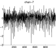
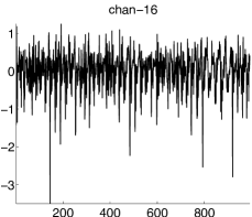
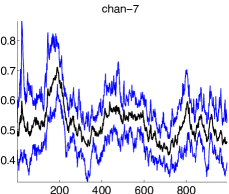
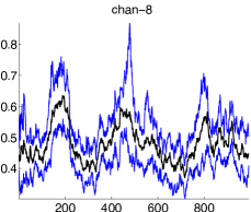
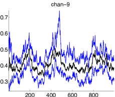
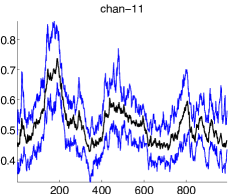
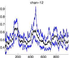
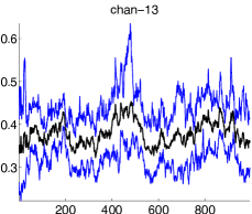
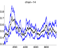
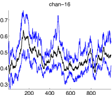
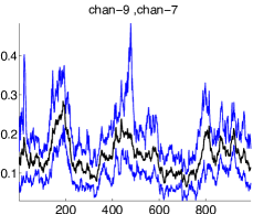
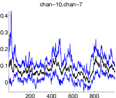
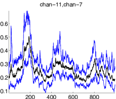
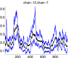
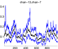
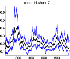
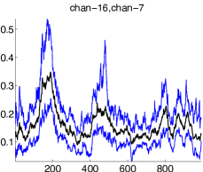
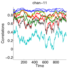
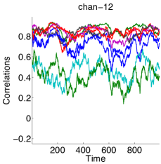
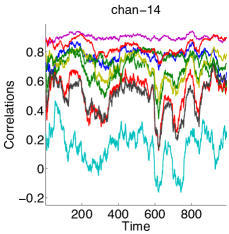
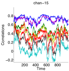
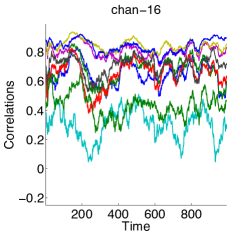
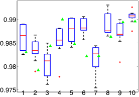
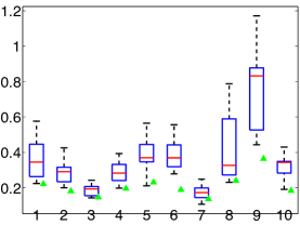
Figure 4 displays volatility trajectories for each of the 10 examined EEG channels showing clear changes in volatility over the 8 seconds of data, while related temporal structure in cross-series covariances is evident in Figure 5. These changes are also captured in Figure 6, which display the time-varying correlations between the EEG channel AR innovations. For the model parameters, Figure 7 shows clear evidence of learning via changes from prior to posterior summaries for the and elements; this figure also highlights the high dependence in the IW-AR(1) model and heterogeneity across EEG channels.

|
|
|
|
|
|
|

|
|
|
|

|
|
|
|
|
 |
7 IW-AR(2) and Higher Order Models
The constructive approach for IW-AR(1) models extends to higher orders. This can be done in a number of ways, as follows.
7.1 Direct Extension
For any order transition distributions of IW-AR() processes can be defined by the conditionals of diagonal blocks of underlying inverse Wishart distributions for matrices. This involves a direct extension of the basic idea underlying the IW-AR(1) model construction. We develop this here for the case of
With begin with
| (7.1) |
where
| (7.2) |
Then, for all ,
| (7.3) | ||||
| (7.4) |
This then constructively defines a stationary order 2 process with common bivariate and univariate margins. In contrast with the IW-AR(1) construction of Section 2, in eqn. (7.1) are not independent over time. Rather, if , then we have defined an autoregressive process on the augmented variance elements:
| (7.5) | ||||
| (7.6) |
The “memory” induced by these off-diagonal elements is evident as the full conditional distribution for is whereas the IW-AR(2) observation model is which involves marginalization over the relevant conditional for the off-diagonal matrices.
As in the case of the IW-AR(1), the construction of eqn. (7.1) implies that
| (7.7) |
with time innovation matrices and independent of and distributed as
| (7.8) | ||||
| (7.9) |
If we assume that such that
| (7.10) |
then
| (7.11) | ||||
| (7.12) |
Furthermore, taking leads to
| (7.13) |
and
| (7.14) | ||||
| (7.15) |
Note that for the specified to be a valid distribution, we need positive definite. As before, this is equivalent to and the Schur complement of being positive definite. Taking and , the Schur complement is simply and
| (7.16) |
So, just as in the IW-AR(1), we require and to be positive definite; the conditions for a valid process and stationarity have not changed in this extension to the IW-AR(2) process based on the chosen parameterization.
More general IW-AR follow from the obvious extension of this constructive approach. Note that the ancillary off-diagonal blocks of the extended matrix defining the IW-AR transition distributions are latent variables that will feature in Bayesian fitting.
7.2 A Second Constructive Approach to Higher-Order Models
A related, alternative and novel approach is defined by coupling AR components to generate higher order AR structures. Specifically, take with having a marginal matrix normal, inverse Wishart form as in the IW-AR model of Section 2. Denote the hyperparameters of this IW-AR(1) by .
Now introduce Markovian dependence into the sequence while maintaining the same conditional independence of on the history of the process. Specifically, take an IW-AR model for so that for each
| (7.17) |
with time innovations having independent matrix normal, inverse Wishart distributions with defining parameters , where .
This induces a second-order Markov model
| (7.18) |
Stationarity of this IW-AR(2) process is implied by simply ensuring the stationarity of the IW-AR(1) process and the embedded IW-AR(1) process: each of and now must be positive definite.
Conditional on earlier defined, we have
| (7.19) |
where and is a deterministic function of the elements of . In the limit as ,
Derivations of these conditional moments are provided in the Appendix.
The new structure of joint distributions of the innovations is to be explored, as are extensions of the MCMC for model fitting.
8 Related Models
A Markov Latent Variable Construction
As discussed in Section 2.3, our IW-AR(1) model in dimensions relates closely to the univariate model arising via a latent variable construction introduced by Pitt et al. (2002); Pitt and Walker (2005). We can extend the univariate model of that reference to the multivariate case, as follows. The process is coupled with a latent variance matrix process via time conditionals: with a Wishart conditional for some and non-singular matrix . It can be shown that this latent variable construction defines a valid joint distribution with margin for all . This leads to an AR(1) transition model in closed form and appears to be the most general AR(1) construction based on the latent variable/process idea of Pitt and Walker (2005).
Although producing identical margins to the IW-AR(1), the proposed multivariate extension of the Pitt and Walker (2005) construction is limited. Such models are always reversible. Most critically, the construction implies , where is scalar. So, in contrast to the matrix of the IW-AR(1), there is no notion of multiple autoregressive coefficients for flexible autocorrelation structures on the elements of . Finally, it is not clear how to extend to higher-order autoregressive models.
Direct Specification of Transition Distributions
The interesting class of models of Philipov and Glickman (2006a) specifies the transition distribution for given as inverse Wishart, discounting information from the previous matrix. Specifically, the conditional mean is given by for some and matrix . The Markov construction generates models with stationary structure. Scaling to higher dimensions, the authors apply the proposed stationary Wishart models to the variance matrix of a lower-dimensional latent factor in a latent factor volatility model (Philipov and Glickman, 2006b), extending prior approaches based on dynamic latent factor models (Aguilar and West, 2000; Aguilar et al., 1999). Based on the specification of Wishart Markov transition kernels, the proposed models do not yield a clear marginal structure and extensions to higher dimensions appear challenging. Furthermore, the proposed sampling-based model fitting strategy yields low acceptance rates in moderate dimensions (e.g., ).
Related approaches in Gouriéroux et al. (2009) define Wishart (and non-central Wishart) processes via functions of sample variance matrices of a collection of latent vector autoregressive processes. Specifically, when the degree of freedom is integer, , with each independently defined via and . For stationary autoregressions, one can analyze the marginal distribution of . Extensions to higher order processes are also presented. For model fitting, the authors rely on a (non-asymptotically efficient) method of moments assuming that a sequence of observed volatility/co-volatility matrices are available. Extensions to embedding the proposed Wishart autoregressive process within a standard stochastic volatility framework is computationally complicated: a mean model can be estimated based on nonlinear filtering approximations of latent volatilities. Within Bayesian analysis of such a setup, the non-central Wishart does not yield an analytic posterior distribution and is challenging to sample. One might be able to exploit latent process constructions, but the analysis is not straightforward.
AR models for Cholesky elements
Several recent works use linear, normal AR(1) models for off-diagonal elements of the Cholesky of and for the log-diagonal elements (Cogley and Sargent, 2005; Primiceri, 2005; Lopes et al., 2010b; Nakajima and West, 2011), building on the Cholesky-based heteroscedastic model of Pourahmadi (1999), and a natural parallel of Bayesian factor models for multivariate volatility (Aguilar and West, 2000; Aguilar et al., 1999). However, each autoregression has an interpretation as the time-varying regression parameters in a model in which the ordering of the elements of the observation vector is required and plays a key role in model formulation. For models in which this is not the case, the parameters employed in the autoregressions are less interpretable. We can cast our IW-AR within a similar framework. The inverse Wishart margins for and translate to Wishart margins for the precision matrices and . Since each Wishart matrix can be equivalently described via an outer product of a collection of identically distributed normal random variables, our IW-AR implicitly arises from a first-order Markov process on the normal random variables and thus defines a Gaussian autoregression, though possibly of a nonlinear form. Note that there are a few key differences between the IW-AR induced element-wise autoregressions and the Cholesky component AR models: (i) the IW-AR autoregressions are on elements of the precision matrix and (ii) these elements comprise a matrix square root, but not the Cholesky square root. The issue of implicitly defining an ordering of observations when using a Cholesky decomposition is not present in the matrix square root considered in the IW-AR case.
9 Final Comments
The structure of the proposed IW-AR processes immediately open possibilities for examining alternative computational methods and extensions to parsimonious modeling of higher-dimensional time series.
The inherent state-space structure of the IW-AR also suggests opportunity to develop more effective computational methods using some variant of particle filtering and particle learning (Carvalho et al., 2010; Lopes et al., 2010a). Among the main challenges here is that of including the fixed parameters – or expanded state variables that include approximate sufficient statistics for these parameters – in particulate representations of filtering distributions (Liu and West, 2001). One possible approach is to harness ideas from particle MCMC (Andrieu et al., 2010). Otherwise, the new IW-AR model class is inherently well-suited to the most effective reweight/resample strategies of particle learning for sequential Monte Carlo.
The inverse Wishart distribution also has extensions to hyper-inverse Wishart (HIW) distributions for variance matrices constrained by specified graphical models (Dawid and Lauritzen, 1993; Carvalho et al., 2007). Graphical models provide scalable structuring for higher-dimensional problems, and it would be interesting to consider extensions of the IW-AR to HIW-AR processes that evolve maintaining the sparsity structure (of the precision matrix) specified by a graphical model.
Appendix A Proofs of Theoretical Properties
A.1 Proof of Theorem 3.3
Let denote the th row of and the th column of . Then, for the IW-AR(1) we can write the element of as
| (A.1) |
Taking the expectation conditioned on ,
| (A.2) |
where we have used the fact that . In matrix form, we have
| (A.3) |
A.2 Proof of Theorem 3.4
For the case of and , we can write eqn. (2.7) as
| (A.12) |
Standard theory implies that
| (A.21) |
The derivation of the conditional mean is exactly as in the general IW-AR case, noting that
A.3 Proof of Theorem 3.5
A.4 Proof of Theorem 3.6
Let such that . According to eqn. (3.9), then shares the same eigenspace as (i.e., the eigenvectors are given by ), and by induction, so does for all . Let denote the diagonal matrix of eigenvalues of . Since , eqn. (3.9) can be rewritten solely in terms of the eigenvalues:
| (A.28) |
In terms of the vectors of eigenvalues , and we have
| (A.29) |
Letting and , we conclude that
| (A.30) |
Since represents a matrix (strictly) convex combination of and , the maximum eigenvalue of is bounded by
| (A.31) |
Here, denotes the maximum eigenvalue of . The term is a rank 1 matrix implying that the only non-zero eigenvalue is equal to . Thus, regardless of , has eigenvalues with modulus strictly less than 1 since has eigenvalues equal to 0 and one equal to . This implies that the conditional mean of the process forgets the initial condition exponentially fast regardless of . Furthermore, since the eigenvalues of have modulus less than 1,
| (A.32) |
implying that, as expected, the eigenvalues of the limiting conditional mean are exactly those of the marginal mean :
| (A.33) | ||||
| (A.34) | ||||
| (A.35) | ||||
| (A.36) |
The last equality follows from matrix inversion and the fact that .
Appendix B Derivation of Forward Filtering Backward Sampling Algorithm
B.1 Approximate Forward Filtering
The inverse Wishart prior on can be analytically updated to an inverse Wishart posterior conditioned on :
| (B.3) |
To propagate to , we use the Chapman-Kolmogorov equation, integrating over :
| (B.4) |
Here, we have used the fact that the transition kernel simply involves independent innovations and deterministically computing . Integrating the elements used to compute (a component of ), the marginal posterior can be derived from the joint posterior of the augmented variance matrix at time given in eqn. (B.3). Although an independent normal-inverse Wishart set of random variables can be combined with a -dimensional inverse Wishart matrix to form a -dimensional inverse Wishart, as discussed in Section 2, there are restrictions on the parameterizations of these respective distributions. The set of distributions specified in eqn. (B.4) do not satisfy these constraints, and thus do not combine to form a -dimensional inverse Wishart distribution on . Namely, the prior and posterior degrees of freedom do not match, nor do the posterior scale matrix and the prior variance term .
Since exact, analytic forward filtering is not possible, we instead approximate the propagate step with a moment-matched inverse Wishart distribution. That is,
| (B.5) |
Based on the approximations made in propagating, the subsequent update step is exact due to the conjugacy of the Gaussian observation and inverse Wishart predictive distribution.
In general, we can choose an arbitrary degree of freedom parameter in our approximate forward filtering. Assume that at time we use degrees of freedom for the moment-matched approximation to the predictive distribution . We use to denote the resulting approximation to the updated posterior .
We initialize at with and
| (B.6) | ||||
Propagating forward,
| (B.7) | ||||
Here, the predictive mean is derived as
| (B.10) |
with . The term is derived via iterated expectations, namely , and employing eqn. (3.9) noting that is conditionally independent of given .
The forward filter then recursively defines
| (B.11) | ||||
with
| (B.12) |
and
| (B.13) |
B.2 Backward Sampling
The density required for backward sampling is the posterior of conditioned on and , which can be written as
| (B.14) | ||||
| (B.15) | ||||
| (B.16) |
Thus, sampling from this conditional posterior is equivalent to fixing in the matrix and sampling a valid conditioned on based on the forward filtering distribution . By valid, we mean a value that corresponds to .
Based on eqn. (5.7),
| (B.21) |
implying that
| (B.26) |
Here, is the forward filtering term defined in eqn. (5.13), with , , denoting the three unique sub-blocks (). The form of eqn. (B.26) allows us to use the previously discussed properties of the inverse Wishart distribution to sample conditioned on and . Specifically, as discussed in Section 2, there exists a such that and
| (B.27) | ||||
with
| (B.28) |
Thus, to sample conditioned on from the approximation to , we first sample as specified in eqn. (B.27) and then compute based on eqn. (B.28).
Appendix C Multivariate t Distribution
The -dimensional multivariate t distribution with degrees of freedom and parameters and has density
| (C.1) |
where
For the proposed IW-AR, since standard theory gives . Marginalizing over in eqn. (4.1), we have
| (C.2) |
Now, implies Marginalizing from the distribution of eqn. (C.2) yields the t distribution with density
| (C.3) |
The marginal likelihood of and given follows immediately.
Appendix D Conditional Mean of IW-AR(2) Model
For the IW-AR(2) process in Section 7.2 we have
| (D.1) |
Since , in deriving the conditional mean of given we first need
| (D.2) | ||||
implying
| (D.3) |
Noting that and since is a deterministic function of the elements of , eqn. (7.19) follows directly. That is,
with as in eqn. (D.1).
In the limit as , we have
Appendix E Sampling for Stochastic Volatility in Time Series Models with IW-AR(1) Components
In eqn. (6.1), the conditional posterior of the autoregressive parameters (i.e., Step 0 of the sampler) is given as follows.
Step 0
Sample the observation autoregressive parameter given and . Assume diagonal defined by the -vector . The autoregressive process of eqn. (6.1) can be equivalently represented as
| (E.1) |
Under a prior , standard theory yields the conditional for as multivariate normal with easily computed moments. For , set .
References
- Aguilar and West (2000) O. Aguilar and M. West. Bayesian dynamic factor models and variance matrix discounting for portfolio allocation. Journal of Business and Economic Statistics, 18:338–357, 2000.
- Aguilar et al. (1999) O. Aguilar, R. Prado, G. Huerta, and M. West. Bayesian inference on latent structure in time series (with discussion). In J.O. Bernardo, J.O. Berger, A.P. Dawid, and A.F.M. Smith, editors, Bayesian Statistics 6, pages 3–26. Oxford University Press, 1999.
- Andrieu et al. (2010) C. Andrieu, A. Doucet, and R. Holenstein. Particle Markov chain Monte carlo methods. Journal of the Royal Statistical Society, Series B, 72(3):269–342, 2010.
- Carvalho et al. (2010) C. M. Carvalho, M. Johannes, H. F. Lopes, and N. G. Polson. Particle learning and smoothing. Statistical Science, 25:88–106, 2010.
- Carvalho et al. (2007) C.M. Carvalho, H. Massam, and M. West. Simulation of hyper-inverse Wishart distributions in graphical models. Biometrika, 94(3):647–659, 2007.
- Chib et al. (2009) S. Chib, Y. Omori, and M. Asai. Multivariate stochastic volatility. In T. G. Andersen, R. A. Davis, J. P. Kreiss, and T. Mikosch, editors, Handbook of Financial Time Series, pages 365–400. Springer-Verlag, Berlin Heidelberg, 2009.
- Cogley and Sargent (2005) T. Cogley and T. J. Sargent. Drifts and volatilities: Monetary policies and outcomes in the post WWII U.S. Review of Economic Dynamics, 8:262–302, 2005.
- Dawid and Lauritzen (1993) A.P. Dawid and S.L. Lauritzen. Hyper-Markov laws in the statistical analysis of decomposable graphical models. The Annals of Statistics, 3:1272–1317, 1993.
- Engle (2002) R. Engle. New frontiers for ARCH models. Journal of Applied Econometrics, 17(5):425–446, 2002.
- Fill and Huber (2001) J.A. Fill and M.L. Huber. The randomness recycler: A new technique for perfect sampling. In Proc. 41th Annual IEEE Symposium on the Foundations of Computer Science, pages 503–511, 2001.
- Freyermuth et al. (2010) J.M. Freyermuth, H. Ombao, and R. von Sachs. Tree-structured wavelet estimation in a mixed effects model for spectra of replicated time series. Journal of the American Statistical Association, 105(490):634–646, 2010.
- Gouriéroux et al. (2009) C. Gouriéroux, J. Jasiak, and R. Sufana. The Wishart autoregressive process of multivariate stochastic volatility. Journal of Econometrics, 150(2):167–181, 2009.
- Harvey et al. (1994) A.C. Harvey, E. Ruiz, and N. Shephard. Multivariate stochastic variance models. Review of Economic Studies, 61:247–264, 1994.
- Krystal et al. (1999a) A. D. Krystal, S. Zoldi, R. Prado, H. S. Greenside, and M. West. The spatiotemporal dynamics of generalized tonic-clonic seizure EEG data: Relevance to the climinal practice of electroconvulsive therapy. In N. Pradhan, P.E. Rapp, and R. Sreenivasan, editors, Nonlinear Dynamics and Brain Functioning. New York: Novascience, 1999a.
- Krystal et al. (2000) A. D. Krystal, M. West, R Prado, H.S. Greenside, S. Zoldi, and R.D. Weiner. The EEG effects of ECT: Implications for rTMS. Depress Anxiety, 12:157–165, 2000.
- Krystal et al. (1999b) A.D. Krystal, R. Prado, and M. West. New methods of time series analysis for non-stationary EEG data: Eigenstructure decompositions of time varying autoregressions. Clinical Neurophysiology, 110(12):2197–2206, 1999b.
- Liu and West (2001) J. Liu and M. West. Combined parameter and state estimation in simulation-based filtering. In A. Doucet, J.F.G. De Freitas, and N.J. Gordon, editors, Sequential Monte Carlo Methods in Practice, pages 197–217. New York: Springer-Verlag, 2001.
- Lopes et al. (2010a) H. F. Lopes, C. M. Carvalho, M. Johannes, and N. G. Polson. Particle learning for sequential Bayesian computation (with discussion). In J.M. Bernardo, M.J. Bayarri, J.O. Berger, A.P. Dawid, D. Heckerman, A.F.M. Smith, and M. West, editors, Bayesian Statistics 9, pages 317 – 360. Oxford University Press, 2010a.
- Lopes et al. (2010b) H. F. Lopes, R. E. McCulloch, and R. Tsay. Cholesky stochastic volatility, booth chicago. Technical report, 2010b.
- Mena and Walker (2005) R.H. Mena and S.G. Walker. Stationary autoregressive models via a Bayesian nonparametric approach. Journal of Time Series Analysis, 26(6):789–805, 2005.
- Nakajima and West (2011) J. Nakajima and M. West. Bayesian dynamic factor models: Latent threshold approach, duke statistical science. Technical report, 2011.
- Ombao et al. (2005) H. Ombao, R. von Sachs, and W. Guo. SLEX analysis of multivariate nonstationary time series. Journal of the American Statistical Association, 100(470):519–531, 2005.
- Philipov and Glickman (2006a) A. Philipov and M.E. Glickman. Multivariate stochastic volatility via Wishart processes. Journal of Business and Economic Statistics, 24(3):313–328, 2006a.
- Philipov and Glickman (2006b) A. Philipov and M.E. Glickman. Factor multivariate stochastic volatility via Wishart processes. Econometric Reviews, 25(2-3):311–334, 2006b.
- Pitt and Walker (2005) M.K. Pitt and S.G. Walker. Constructing stationary time series models using auxiliary variables with applications. Journal of the American Statistical Association, 100(470):554–564, 2005.
- Pitt et al. (2002) M.K. Pitt, C. Chatfield, and S.G. Walker. Constructing first order stationary autoregressive models via latent processes. Scandinavian Journal of Statistics, 29(4):657–663, 2002.
- Pourahmadi (1999) M. Pourahmadi. Joint mean-covariance models with applications to longitudinal data: Unconstrained parameterisation. Biometrika, 86(3):677–690, 1999.
- Prado and West (1997) R. Prado and M. West. Exploratory modelling of multiple non-stationary time series: Latent process structure and decompositions. In T. Gregoire, editor, Modelling Longitudinal and Spatially Correlated Data, pages 349–362. Springer-Verlag, 1997.
- Prado and West (2010) R. Prado and M. West. Time Series: Modelling, Computation and Inference. Chapman & Hall/CRC Press, The Taylor Francis Group, 2010. ISBN 978-1-420093360.
- Prado et al. (2001) R. Prado, M. West, and A. D. Krystal. Multi-channel EEG analyses via dynamic regression models with time-varying lag/lead structure. Journal of the Royal Statistical Society (Ser. C), 50:95–110, 2001.
- Primiceri (2005) G. E. Primiceri. Time varying structural vector autoregressions and monetary policy. Review of Economic Studies, 72:821–852, 2005.
- Quintana and West (1987) J. M. Quintana and M. West. An analysis of international exchange rates using multivariate DLMs. The Statistician, 36:275–281, 1987.
- Quintana (1992) J.M. Quintana. Optimal portfolios of forward currency contracts. In J. O. Berger, J. M. Bernardo, A. P. Dawid, and A. F. M. Smith, editors, Bayesian Statistics IV, pages 753–762. Oxford University Press, 1992.
- Quintana et al. (2003) J.M. Quintana, V. Lourdes, O. Aguilar, and J. Liu. Global gambling. In J. M. Bernardo, M. J. Bayarri, J. O. Berger, A. P. Dawid, D. Heckerman, A. F. M. Smith, and M. West, editors, Bayesian Statistics VII, pages 349–368. Oxford University Press, 2003.
- Quintana et al. (2010) J.M. Quintana, C. M. Carvalho, J. Scott, and T. Costigliola. Futures markets, Bayesian forecasting and risk modelling. In A. O’Hagan and M. West, editors, The Handbook of Applied Bayesian Analysis, pages 343–365. Oxford University Press, 2010.
- Uhlig (1994) H. Uhlig. On singular Wishart and singular multivariate beta distributions. Annals of Statistics, 22:395–405, 1994.
- West and Harrison (1997) M. West and P.J. Harrison. Bayesian Forecasting and Dynamic Models. Springer-Verlag, New York, 1997.
- West et al. (1999) M. West, R. Prado, and A. D. Krystal. Evaluation and comparison of EEG traces: Latent structure in non-stationary time series. Journal of the American Statistical Association, 94:1083–1095, 1999.