Electron-acoustic solitary waves in the presence of a suprathermal electron component

Abstract

The nonlinear dynamics of electron-acoustic localized structures in a collisionless and unmagnetized plasma consisting of “cool” inertial electrons, “hot” electrons having a kappa distribution, and stationary ions is studied. The inertialess hot electron distribution thus has a long-tailed suprathermal (non-Maxwellian) form. A dispersion relation is derived for linear electron-acoustic waves. They show a strong dependence of the charge screening mechanism on excess suprathermality (through $\kappa$). A nonlinear pseudopotential technique is employed to investigate the occurrence of stationary-profile solitary waves, focusing on how their characteristics depend on the spectral index $\kappa$, and the hot-to-cool electron temperature and density ratios. Only negative polarity solitary waves are found to exist, in a parameter region which becomes narrower as deviation from the Maxwellian (suprathermality) increases, while the soliton amplitude at fixed soliton speed increases. However, for a constant value of the true Mach number, the amplitude decreases for decreasing $\kappa$.

year number number identifier

I Introduction

Electron-acoustic waves may occur in plasmas characterized by a co-existence of two distinct electron populations, here referred to as “cool” and “hot” electrons. These are electrostatic waves of high frequency (in comparison with the ion plasma frequency), propagating at a phase speed which lies between the hot and cool electron thermal velocities. On such a fast (high frequency) dynamical scale, the positive ions may safely be assumed to form a uniform stationary charge background simply providing charge neutrality, yet playing no essential role in the dynamics. The cool electrons provide the inertia necessary to maintain the electrostatic oscillations, while the restoring force comes from the hot electron pressure.

A matter of importance in electrostatic wave propagation (although inevitably overlooked in fluid plasma models) is Landau damping, which becomes stronger when the phase velocity approaches the thermal velocity of either electron component, thus the wave can propagate in the plasma only within a restricted range of parameter values. It turns out that electron-acoustic waves are weakly damped for a temperature ratio $T_{c}/T_{h}\lesssim 0.1$ and provided that the cool electrons represent an intermediate fraction of the total electron density: $0.2\lesssim n_{c}/(n_{c}+n_{h})\lesssim 0.8$. Tokar1984 ; Gary1985 ; Mace1990 ; Berthomier1999 The wavenumber $k$ to minimize damping lies roughly between $0.2\lambda_{Dc}^{-1}$ and $0.6\lambda_{Dc}^{-1}$ (where $\lambda_{Dc}$ is the cool electron Debye length). These results on bi-Maxwellian plasmas were later extended to include the effect of the excess suprathermality of the hot electrons Mace1999 (a physical feature to be discussed below). It was found that excess suprathermal electrons do cause a modification of the damping curves, but the overall qualitative conclusion remains unchanged: electron-acoustic waves survive Landau damping over a wide range of parameter values. Mace1999 However, care must be taken in the choice of plasma configuration when studying nonlinear electron-acoustic structures, so as to ensure that one is considering a region of parameter space in which Landau damping is minimized.

Electron-acoustic waves occur in laboratory experiments Henry1972 ; Ikezawa1981 and space plasmas, e.g., in the Earth’s bow shock Thomsen1983 ; Feldman1983 ; Bale1998 and in the auroral magnetosphere Tokar1984 ; Lin1984 . They are associated with Broadband Electrostatic Noise (BEN), a common high-frequency background activity, regularly observed by satellite missions in the plasma sheet boundary layer (PSBL) Matsumoto1994 ; Cattell1999 ; Kakad2009 . BEN emission includes a series of isolated bipolar pulses, within a frequency range from $\sim 10$ Hz up to the local electron plasma frequency ($\sim 10$ kHz) Matsumoto1994 . This clearly suggests that BEN is related to electron dynamics rather than to the ions Matsumoto1994 ; Kakad2009 .

In the standard bi-Maxwellian picture, the two electron species would each be assumed to be in a (different) thermal Maxwellian distribution, parameterized via two distinct temperature values, $T_{c}$ and $T_{h}$, respectively Watanabe1977 ; Nishihara1981 ; Berthomier1998 . Contrary to this picture, space and laboratory plasmas often possess an excess population of suprathermal electrons, a fact which is reflected in a power law distribution at high velocity (above the electron thermal speed). This excess suprathermality phenomenon is well modeled by a generalized Lorentzian or $\kappa$-distribution Summers1991 ; Hellberg2000 ; Baluku2008 ; Hellberg2009 ; Pierrard2010 . The common form of the isotropic (three-dimensional) generalized Lorentzian or $\kappa$-distribution function is given by Summers1991 ; Baluku2008 ; Hellberg2009

$$f_{\kappa}(v)=n_{0}(\pi\kappa\theta^{2})^{-3/2}\frac{\Gamma(\kappa+1)}{\Gamma(\kappa-\frac{1}{2})}\left(1+\frac{v^{2}}{\kappa\theta^{2}}\right)^{-\kappa-1},$$ (1)

where $n_{0}$ is the equilibrium number density of the electrons, $v$ the velocity variable, and $\theta$ the most probable speed, which acts as a characteristic “modified thermal speed”, and is related to the usual thermal speed $v_{th,e}=(2k_{B}T_{e}/m_{e})^{1/2}$ by $\theta=v_{th,e}\left[(\kappa-\tfrac{3}{2})/\kappa\right]^{1/2}$. Here $k_{B}$ is the Boltzmann constant, $m_{e}$ the electron mass and $T_{e}$ the temperature of an equivalent Maxwellian having the same energy content. Hellberg2009 The term involving the Gamma function ($\Gamma$) arises from the normalization of $f_{\kappa}(v)$, viz., $\int f_{\kappa}(v)d^{3}v=n_{0}$. Here, suprathermality is denoted by the spectral index $\kappa$, with $\kappa>\frac{3}{2}$, for reality of the most probable speed, $\theta$. Hellberg2009 Low values of $\kappa$ are associated with a significant number of suprathermal particles; on the other hand, for $\kappa\rightarrow\infty$ a Maxwellian distribution is recovered.

The $\kappa$-distribution was first applied to model velocity distributions observed in space plasmas that were Maxwellian-like at lower velocities, but had a power-law form at higher speeds Vasyliunas1968 , and was later applied in a variety of studies, successfully fitting many real space observations, e.g., Feldman1983 ; Christon1988 ; Pierrard1996 ; Pierrard2010 . Typical $\kappa$ values usually lie in the range $2<\kappa<6$. For example, observations in the earth’s foreshock satisfy $3<\kappa_{e}<6$, Feldman1983 measurements of plasma sheet electron and ion distributions yield $\kappa_{i}=4.7$ and $\kappa_{e}=$ $5.5$ (here, $e$ denotes electrons and $i$ ions), Christon1988 and coronal electrons in the solar wind are modeled with $2<\kappa_{e}<6$ Pierrard1996 . Recent observations of the radial distribution of the electron population in Saturn’s magnetosphere also point towards a kappa distribution ($\kappa_{e}\simeq 2.9$ - $4.2)$ Schippers2008 . Therefore, we focus our interest in the following on the range $2<\kappa<6$; in fact, the Maxwellian limit is already practically attained for values above $\kappa\simeq 10$.

A linear analysis of electron-acoustic waves was first carried out by assuming an unmagnetized Maxwellian homogeneous plasma, which exhibited a heavily damped acoustic-like solution in addition to Langmuir waves and ion-acoustic waves. Fried1961 Those early results were later extended to take into account the effect of excess suprathermal particles Mace1999 ; Hellberg2002 , whose presence in fact results in an increase in the Landau damping at small wavenumbers, in particular when the hot electron component is dominant Mace1999 ; Baluku2011 . Studies of linear and nonlinear electron-acoustic waves in plasmas with nonthermal electrons have received a great deal of interest in recent years Dubouloz1991 ; Singh2004 ; Kourakis2004 ; Cattaert2005 ; Verheest2005 . Negative potential solitary structures were shown to exist in a two-electron plasma, either for Maxwellian Dubouloz1991 or for nonthermal Singh2004 ; Sultana2010 hot electrons. Interestingly, either incorporation of finite inertia Cattaert2005 ; Verheest2005 or the addition of a beam component Berthomier2000 ; Mace2001 may lead to the existence of positive and negative potential solitons. A recent investigation has established the properties of modulated electron-acoustic wavepackets in kappa-distributed plasmas, and has studied the effect of suprathermality on the amplitude (modulational) stability. Sultana2011

In this paper, we study the linear and nonlinear dynamics of electron-acoustic waves in a plasma consisting of cool adiabatic electron and hot $\kappa$-distributed electrons, in addition to stationary ions. The paper is organised as follows. An electron-plasma-fluid model is presented in Section II. In Section III, a linear dispersion relation is derived and discussed. In Section IV, the Sagdeev pseudopotential method is employed to investigate the occurrence of stationary profile electrostatic solitary waves. In Section V, we depict the existence domain of the electron-acoustic solitary waves. Section VI is devoted to a parametric investigation of the form of the Sagdeev pseudopotential and of the characteristics of electron-acoustic solitary waves. Our results are summarized in Section VII.

II Model Equations

We consider a plasma consisting of three components, namely a cool electron-fluid (at temperature $T_{c}\neq 0$), an inertialess hot electron component with a nonthermal ($\kappa$) velocity distribution, and uniformly distributed stationary ions.

The cool electron behavior is governed by the continuity equation,

$$\frac{\partial n_{c}}{\partial t}+\frac{\partial(n_{c}u_{c})}{\partial x}=0,$$ (2)

and the momentum equation

$$\frac{\partial u_{c}}{\partial t}+u_{c}\frac{\partial u_{c}}{\partial x}=\frac{e}{m_{e}}\frac{\partial\phi}{\partial x}-\frac{1}{m_{e}n_{c}}\frac{\partial p_{c}}{\partial x}\,.$$ (3)

The pressure of the cool electrons is governed by

$$\frac{\partial p_{c}}{\partial t}+u_{c}\frac{\partial p_{c}}{\partial x}+\gamma p_{c}\frac{\partial u_{c}}{\partial x}=0\,.$$ (4)

Here $n_{c}$, $u_{c}$ and $p_{c}$ are the number density, the velocity and the pressure of the cool electron fluid, $\phi$ is the electrostatic wave potential, $e$ the elementary charge, and $\gamma=(f+2)/f$ denotes the specific heat ratio (for $f$ degrees of freedom). We shall assume $\gamma=3$ (viz., $f=1$ in 1D) for the adiabatic cool electrons.

We assume the ions to be stationary (immobile), i.e., in a uniform state $n_{i}=n_{i,0}=$ const. (where $n_{i,0}$ is the undisturbed ion density) at all times. In order to obtain an expression for the number density of the hot electrons, $n_{h}$, based on the $\kappa$ distribution (1), one may integrate Eq. (1) over the velocity space, to obtain Baluku2008

$$n_{h}(\phi)=n_{h,0}\left(1-\frac{e\phi}{k_{B}T_{h}(\kappa-\tfrac{3}{2})}\right)^{-\kappa+1/2}\,,$$ (5)

where $n_{h,0}$ and $T_{h}$ are the equilibrium number density and “temperature” of the hot electrons, respectively, and $\kappa$ is the spectral index measuring the deviation from thermal equilibrium.

The densities of the ($\kappa$-distributed) hot electrons, the adiabatic cool electrons, and the stationary ions are coupled via Poisson’s equation:

$$\frac{\partial^{2}\phi}{\partial x^{2}}=-\frac{e}{\varepsilon_{0}}\left(Zn_{i}-n_{c}-n_{h}\right),$$ (6)

where $\varepsilon_{0}$ is the permittivity constant, $n_{h}$ and $n_{i}$ are the number density of hot electrons and ions, respectively.

At equilibrium, the plasma is quasi-neutral, so that

$$n_{c,0}+n_{h,0}=Zn_{i,0}\,,$$ (7)

implying $Z{n_{i,0}}/{n_{c,0}}=1+\beta$, where we have defined the hot-to-cool electron density ratio

$$\beta=\frac{n_{h,0}}{n_{c,0}}.$$ (8)

According to Ref. Tokar1984, , Landau damping is minimized in the range $0.2\lesssim n_{c,0}/(n_{c,0}+n_{h,0})\lesssim 0.8$, implying $0.25\leqslant\beta\leqslant 4$. This is our region of interest in what follows, as nonlinear structures will not be sustainable for plasma configurations for which the linear waves are strongly damped.

Scaling by appropriate quantities, we obtain the normalized set of equations

$$\frac{\partial n}{\partial t}+\frac{\partial(nu)}{\partial x}=0,$$ (9)

$$\frac{\partial u}{\partial t}+u\frac{\partial u}{\partial x}=\frac{\partial\phi}{\partial x}-\frac{\sigma}{n}\frac{\partial p}{\partial x},$$ (10)

$$\frac{\partial p}{\partial t}+u\frac{\partial p}{\partial x}+3p\frac{\partial u}{\partial x}=0,$$ (11)

$$\frac{\partial^{2}\phi}{\partial x^{2}}=n+\beta\left[1-\frac{\phi}{\kappa-3/2}\right]^{-\kappa+1/2}-\beta-1.$$ (12)

Here, $n$, $u$ and $p$ denote the cool electron fluid density, velocity and pressure variables normalized with respect to $n_{c,0}$, $c_{th}=\left[k_{B}T_{h}/m_{e}\right]^{1/2}$ and $n_{c,0}k_{B}T_{c}$, respectively. Time and space were scaled by the plasma period $\omega_{pc}^{-1}=(n_{c,0}e^{2}/\varepsilon_{0}m_{e})^{-1/2}$ and the characteristic length $\lambda_{0}=(\varepsilon_{0}k_{B}T_{h}/n_{c,0}e^{2})^{1/2}$, respectively. Finally, $\phi$ is the wave potential scaled by $k_{B}T_{h}/e$. We have defined the temperature ratio of the cool to the hot electrons as

$$\sigma=T_{c}/T_{h}.$$ (13)

III Linear waves

As a first step, we linearize Eqs. (9)-(12), to study small-amplitude harmonic waves of frequency $\omega$ and wavenumber $k$. The linear dispersion relation for electron-acoustic waves then reads:

$$\omega^{2}=\frac{k^{2}}{k^{2}+k_{D,\kappa}^{2}}+3{\sigma}k^{2}\,,$$ (14)

where $\sqrt{3\sigma}$ is essentially the (normalized) cool electron thermal velocity. After taking account of differences in normalization, this agrees with the form found in Sahu2010 .

We note the appearance of a normalized $\kappa$-dependent screening factor (scaled Debye wavenumber) $k_{D,\kappa}$ in the denominator, defined by

$$k_{D,\kappa}\equiv\dfrac{1}{\lambda_{D,\kappa}}\equiv\left[\dfrac{\beta(\kappa-\frac{1}{2})}{\kappa-\tfrac{3}{2}}\right]^{1/2}\,.$$ (15)

Since this is the inverse of the (Debye) screening length, we notice that the latter in fact decreases due to an excess in suprathermal electrons (i.e., $\lambda_{D,\kappa}<\lambda_{D,\infty}$ for any finite value of $\kappa$). This is in agreement with Refs. Chateau1991, ; Bryant1996, ; Mace1998, ; note also the discussion in Ref. Sultana2010, .

From Eq. (14), we see that the frequency $\omega(k)$, and hence also the phase speed, increases with higher temperature ratio $\sigma=T_{c}/T_{h}$. However, this is usually a small correction to the dominant first term on the righthand side of (15). For large wavelength values (small $k\ll k_{D,\kappa}$), the phase speed is given by

$$v_{ph}\simeq\left[\dfrac{\kappa-\tfrac{3}{2}}{\beta(\kappa-\frac{1}{2})}+3\sigma\right]^{1/2}\,,$$ (16)

while on the other hand, the thermal contribution is dominant for high wavenumber $k\gg k_{D,\kappa}$, i.e.

$$v_{ph}\simeq(3\sigma)^{1/2}.$$ (17)

However, we should recall from kinetic theoryTokar1984 ; Gary1985 ; Mace1990 ; Mace1999 that both for very long wavelengths ($k\lambda_{Dc}\lesssim 0.2$) and very short wavelengths ($k\lambda_{Dc}\geq 0.6$), the wave is strongly damped, and thus these limits may be of academic interest only. The mode is weakly damped only for intermediate wavelength values, where its acoustic nature is not manifest. Tokar1984 ; Gary1985 ; Mace1990 ; Mace1999 ; Baluku2011 Here, $\lambda_{Dc}=(\varepsilon_{0}k_{B}T_{c}/n_{c,0}e^{2})^{1/2}$ is the cool electron Debye length.

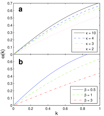
Figure 1: (Color online) Dispersion curve for harmonic (linear) electron-acoustic waves. Upper panel: The variation of the dispersion curve for different values of  $\kappa$ is depicted. Curves from top to bottom: $\kappa=10$  (solid), $4$ (dashed), $3$ (dot-dashed), and $2$ (dotted curve). Here, $\sigma=0.01$ and $\beta=1$. Bottom panel: Variation of the dispersion curve for different values of  $\beta$. Curves from top to bottom: $\beta=0.5$ (solid), $1$ (dashed), and $3$ (dot-dashed curve). Here, $\sigma=0.01$ and $\kappa=3$.

Restoring dimensions for a moment, the dispersion relation becomes

$$\omega^{2}=\omega_{pc}^{2}\frac{k^{2}\lambda_{Dh}^{2}}{k^{2}\lambda_{Dh}^{2}+\dfrac{\kappa-\frac{1}{2}}{\kappa-\tfrac{3}{2}}}+3k^{2}c_{tc}^{2}.$$ (18)

where $c_{tc}=(k_{B}T_{c}/m_{e})^{1/2}$ is the cool electron thermal speed and $\lambda_{Dh}$ is the hot electron Debye length defined by

$$\lambda_{Dh}=\left(\dfrac{\varepsilon_{0}k_{B}T_{h}}{n_{h,0}e^{2}}\right)^{1/2}=\beta^{-1/2}\lambda_{0}.$$ (19)

It appears appropriate to compare the above results with earlier results, in the linear regime. First of all, we note that Ref. Mace1999, has adopted a kinetic description of electron-acoustic waves in suprathermal plasmas. For this purpose, Eq. (18) may be cast in the form,

$$\omega^{2} =k^{2}\left(\frac{C_{s\kappa}^{2}}{1+k^{2}\lambda_{\kappa h}^{2}}+3c_{tc}^{2}\right)$$

$$=\omega_{pc}^{2}\frac{1+3k^{2}\lambda_{Dc}^{2}+3\lambda_{Dc}^{2}/\lambda_{\kappa h}^{2}}{1+1/k^{2}\lambda_{\kappa h}^{2}}\,.$$ (20)

Here $C_{s\kappa}^{2}=\omega_{pc}^{2}\lambda_{\kappa h}^{2}=(n_{c,0}/n_{h,0})[(\kappa-3/2)/(\kappa-1/2)]c_{th}^{2}$ is the electron acoustic speed in a suprathermal plasma, while the effective shielding length is given by $\lambda_{\kappa h}^{2}=[\epsilon_{0}k_{B}T_{h}/n_{h,0}e^{2}][(\kappa-3/2)/(\kappa-1/2)]$. Our Eq. (20) above agrees with relation (3) in Ref. Mace1999, (upon considering the limit $\lambda_{Dc}\rightarrow 0$ therein). In the limit $\kappa\rightarrow\infty$ (Maxwellian distribution), Eq. (20) recovers precisely Eq. (1) in Ref. Berthomier2000, , upon considering the limit $\lambda_{Dc}\rightarrow 0$. Furthermore, one recovers exactly Eq. (5) in Ref. Kakad2009, for Maxwellian plasma in the cold-electron limit ($T_{c}{=0}$).

In Figure 1, we depict the dispersion curve of the electron-acoustic mode, showing the effect of varying the values of the spectral index $\kappa$ and the density ratio $\beta$. It is confirmed numerically that the phase speed ($\omega/k$) increases weakly with a reduction in suprathermal particle excess, as the Maxwellian is approached, and that there is a significant reduction in phase speed as the plasma model changes from one in which the cool electrons dominate, to one which is dominated by the hot electron density.

IV Nonlinear analysis for large amplitude solitary waves

Anticipating constant profile solutions, we shall consider Eqs. (9)–(12) in a stationary frame traveling at a constant normalized velocity $M$ (to be referred to as the Mach number), implying the transformation $\xi=x-Mt$. The space and time derivatives are thus replaced by $\partial/\partial x=d/d\xi$ and $\partial/\partial t=-Md/d\xi$, respectively, so Eqs. (9)–(12) take the form:

$$-M\dfrac{dn}{d\xi}+\frac{d(nu)}{d\xi}=0,$$ (21)

$$-M\dfrac{du}{d\xi}+u\dfrac{du}{d\xi}=\dfrac{d\phi}{d\xi}-\frac{\sigma}{n}\dfrac{dp}{d\xi},$$ (22)

$$-M\dfrac{dp}{d\xi}+u\dfrac{dp}{d\xi}+3p\dfrac{du}{d\xi}=0,$$ (23)

$$\frac{d^{2}\phi}{d\xi^{2}}=-(\beta+1)+n+\beta\left[1-\frac{\phi}{(\kappa-\tfrac{3}{2})}\right]^{-\kappa+1/2}.$$ (24)

We assume that the equilibrium state is reached at both infinities ($\xi\rightarrow\pm\infty$). Accordingly, we integrate and apply the boundary conditions $n=1$, $p=1$, $u=0$ and $\phi=0$ at $\pm\infty$. One thus obtains

$$u=M\left(1-\frac{1}{n}\right),$$ (25)

$$u={M-(M}^{2}{+2\phi-3n^{2}\sigma+3\sigma)}^{1/2},$$ (26)

and

$$p=n^{3}.$$ (27)

Combining Eqs. (25)–(27), we obtain the following biquadratic equation for the cool electron density,

$${3\sigma n^{4}}-({M}^{2}{+2\phi+3\sigma)n^{2}}+{M}^{2}=0\,.$$ (28)

The solution of Eq. (28) may be written as

$${n=}\dfrac{1}{2}\left(n_{(+)}\pm n_{(-)}\right),$$ (29)

where

$$n_{(+)} {\equiv}\left[\dfrac{{2\phi+}\left({M+}\sqrt{3{\sigma}}\right)^{2}}{3{\sigma}}\right]^{1/2},$$ (30)

$$n_{(-)} {\equiv}\left[\dfrac{{2\phi+\left({M-}\sqrt{3{\sigma}}\right)^{2}}}{3{\sigma}}\right]^{1/2}.$$ (31)

From the boundary conditions, $n=1$ at $\phi=0$, it follows that the negative sign must be taken in Eq. (29). Furthermore, we shall assume that $M>\sqrt{3\sigma}$, i.e., that the cool electrons are supersonic, while the hot electrons are subsonic, thus we require that $M<1$.

Reality of the density variable imposes the requirement ${2\phi+\left({M-}\sqrt{3{\sigma}}\right)^{2}>0}$, which implies a limit on the electrostatic potential value $|\phi_{\max}|=\frac{1}{2}\left({M-}\sqrt{3{\sigma}}\right)^{2}$ associated with negative solitary structures (positive electric potentials, should they exist, satisfy the latter condition automatically, and are thus not limited).

Substituting the density expression (29)–(31) into Poisson’s equation (24) and integrating, yields the pseudo-energy balance equation for a unit mass in a conservative force field, if one defines $\xi$ as “time” and $\phi$ as “position” variable:

$$\frac{1}{2}\left(\frac{d\phi}{d\xi}\right)^{2}+\Psi(\phi)=0,$$ (32)

where the Sagdeev pseudopotential $\Psi(\phi)$ is given by

$$\Psi(\phi) =\beta\left[1-\left(1+\frac{\phi}{-\kappa+\tfrac{3}{2}}\right)^{-\kappa+3/2}\right]+(1+\beta)\phi$$

$$+\frac{1}{6\sqrt{3{\sigma}}}\left[\left({M+}\sqrt{3{\sigma}}\right)^{3}-{{\left({M-}\sqrt{3{\sigma}}\right)^{3}}}\right.$$

$$-\left({2\phi+}\left[{M+}\sqrt{3{\sigma}}\right]^{2}\right)^{3/2}$$

$$\left.+{\left({2\phi+\left[{M-}\sqrt{3{\sigma}}\right]^{2}}\right)}^{3/2}\right].$$ (33)

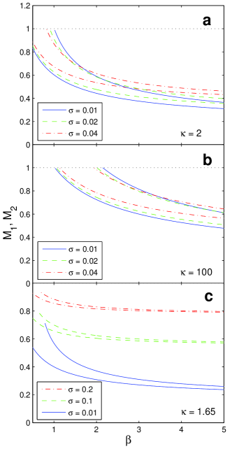
Figure 2: (Color online) Variation of the lower limit $M_{1}$ (lower curves) and the upper limit $M_{2}$ (upper curves) with the hot-to-cold electron density ratio $\beta$ for different values of the temperature ratio $\sigma$. Solitons may exist for values of the Mach number $M$ in the region between the lower and the upper curve(s) of the same style/color. Curves: (a-b) $\sigma=0.01$ (solid), $0.02$ (dashed), and $0.04$ (dot-dashed), and (c) $\sigma=0.01$ (solid), $0.1$ (dashed), and $0.2$ (dot-dashed) Here, we have taken: (a) $\kappa=2$, (b) $\kappa=100$ (quasi-Maxwellian), and (c) $\kappa=1.65$.

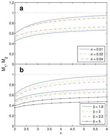
Figure 3: (Color online) Variation of the lower limit $M_{1}$ (lower curves) and the upper limit $M_{2}$ (upper curves) with the suprathermality parameter $\kappa$ for different values of the temperature ratio $\sigma$ (upper panel), and density ratio $\beta$ (bottom panel). Solitons may exist for values of the Mach number $M$ in the region between the lower and upper curves of the same style/color. Upper panel: $\sigma=0.01$ (solid curve), $0.02$ (dashed), and $0.04$ (dot-dashed). Here, we have taken $\beta=2$. Lower panel: $\beta=1.8$ (solid), $2$ (dashed), $2.2$ (dot-dashed), and $5$ (solid circles). Here, $\sigma=0.02$.

V Soliton existence domain

We next investigate the conditions for existence of solitons. First, we need to ensure that the origin at $\phi=0$ is a root and a local maximum of $\Psi$ in Eq. (33), i.e., $\Psi(\phi)=0$, $\Psi^{\prime}(\phi)=0$ and $\Psi^{\prime\prime}(\phi)<0$ at $\phi=0$ Verheest2004 ; McKenzie2004 ; Verheest2007 , where primes denote derivatives with respect to $\phi$. It is easily seen that the first two constraints are satisfied. We thus impose the condition

$$F_{1}(M)=-\left.\Psi^{\prime\prime}(\phi)\right|_{\phi=0}=\frac{\beta(\kappa-\frac{1}{2})}{\kappa-\tfrac{3}{2}}-\frac{1}{M^{2}-3{\sigma}}>0.$$ (34)

Eq. (34) provides the minimum value for the Mach number, $M_{1}$, i.e. :

$$M>M_{1}=\left[\frac{\kappa-\tfrac{3}{2}}{\beta(\kappa-\frac{1}{2})}+3{\sigma}\right]^{1/2}.$$ (35)

Clearly, $M_{1}$ is the (normalized) electron-acoustic phase speed – cf. Eq. (16). It is thus also related to Debye screening via the screening parameter $\lambda_{D,\kappa}$ in (15), associated with the hot $\kappa$-distributed electrons. We deduce that soliton solutions are super-acoustic. For Maxwellian hot electrons ($\kappa\rightarrow\infty$) and cold “cool” electrons ($\sigma=0$), we obtain $M_{1}=1/\beta^{1/2}$, thus recovering the normalized phase speed for electron-acoustic waves in a Maxwellian plasma. Mace1999 The lower Mach number limit, $M_{1}$, increases with $T_{c}$ (via $\sigma$), and decreases for lower values of $\kappa$ (large excess of suprathermal electrons), and hence the sound speed in suprathermal plasmas is reduced, in comparison with Maxwellian plasmas ($\kappa\rightarrow\infty$).

An upper limit for $M$  is found through the fact that the cool electron density becomes complex at $\phi=\phi_{max}$, and hence the largest soliton amplitude satisfies $F_{2}(M)=\Psi(\phi)|_{\phi=\phi_{\max}}>0$. This yields the following equation for the upper limit in M:

$$F_{2}(M) =-\frac{1}{2}(1+\beta)\left({M-}\sqrt{3{\sigma}}\right)^{2}-\frac{4}{3}M^{3/2}\left(3{\sigma}\right)^{1/4}$$

$$+\beta\left(1-\left[1+\frac{\left({M-}\sqrt{3{\sigma}}\right)^{2}}{2\kappa-3}\right]^{-\kappa+3/2}\right)$$

$$+M{{{}^{2}+}\sigma}=0\,.$$ (36)

Solving Eq. (36) provides the upper limit $M_{2}(\kappa,\beta,\sigma)$ for acceptable values of the Mach number for solitons to exist.

For comparison, for a Maxwellian distribution (here recovered as $\kappa\rightarrow\infty$), the constraints reduce to

$$F_{1}(M) =\beta-\frac{1}{M^{2}-3{\sigma}}>0,$$ (37)

$$F_{2}(M) =-\frac{1}{2}(1+\beta)\left({M-}\sqrt{3{\sigma}}\right)^{2}-\frac{4}{3}M^{3/2}\left(3{\sigma}\right)^{1/4}$$

$$+\beta\left(1-\exp\left[-\tfrac{1}{2}\left({M-}\sqrt{3{\sigma}}\right)^{2}\right]\right)$$

$$+M{{{}^{2}+}\sigma}>0.$$ (38)

The latter equation provides the upper limit $M_{2}$, while the lower limit becomes $M_{1}=(1/\beta+3\sigma)^{1/2}$.

In the opposite limit of ultrastrong suprathermality, i.e., $\kappa\rightarrow 3/2$, the Mach number threshold approaches a non-zero limit $M_{1}=\sqrt{3{\sigma}}$, which is essentially the thermal speed, as noted above (recall that $M>\sqrt{3{\sigma}}$ by assumption). The upper limit $M_{2}$ is then given by

$$F_{2}(M) =-\frac{1}{2}(1+\beta)\left({M-}\sqrt{3{\sigma}}\right)^{2}+M{{{}^{2}+}\sigma}$$

$$-\frac{4}{3}M^{3/2}\left(3{\sigma}\right)^{1/4}=0\,.$$ (39)

Interestingly, the two limits $M_{1}$ and $M_{2}$ both tend to the same limit as $\kappa\rightarrow 3/2$, namely, $\sqrt{3{\sigma}}$, where the soliton existence region vanishes, as the kappa distribution breaks down.

We have studied the existence domain of electron-acoustic solitary waves for different values of the parameters. The results are depicted in Figs. 2–3. Solitary structures of the electrostatic potential may occur in the range $M_{1}<M<M_{2}$, which depends on the parameters $\beta$, $\kappa$, and $\sigma$. We recall that we have also assumed that cool electrons are supersonic (in the sense $M>\sqrt{3{\sigma}}$) Verheest2004 ; McKenzie2004 ; Verheest2007 , and the hot electrons subsonic ($M<1$), and care must be taken not to go beyond the limits of the plasma model.

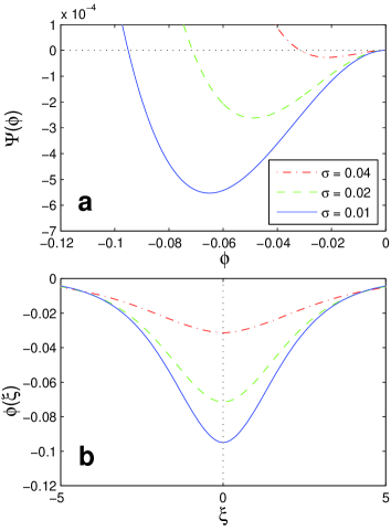
Figure 4: (Color online) The pseudopotential $\Psi(\phi)$ (upper panel) and the associated solution (electric potential pulse) $\phi$ (lower panel) are depicted versus position $\xi$, for different values of the temperature ratio $\sigma\,$. We have taken: $\sigma=0.01$ (solid curve), $0.02$ (dashed curve), and $0.04$ (dot-dashed curve). The other parameter values are $\beta=1.3$, $\kappa=2.5$ and $M=0.75$.

The interval $[M_{1},M_{2}]$ where solitons may exist is depicted in Fig. 2, in two opposite cases: in (a) and (c) two very low, and in (b) one very high value of $\kappa$. We thus see that for both a quasi-Maxwellian distribution and one with a large excess suprathermal component of hot electrons, both $M_{1}$ and $M_{2}$ decrease with an increase in the relative density parameter $\beta$ for fixed $\kappa$ and soliton speed $M$. Further, the upper limit falls off more rapidly, and thus the existence domain in Mach number becomes narrower for higher values of the hot-to-cool electron density ratio. Comparing the two frames (a) and (b) in Fig. 2, we immediately notice that suprathermality (low $\kappa$) results in solitons propagating at lower Mach number values, a trend which is also seen in Fig. 2c. Another trend that is visible in Figs. 2–3a is that increased thermal pressure effects of the cool electrons, manifested through increasing $\sigma$, also lead to a narrowing of the Mach number range that can support solitons. Finally, we note that for $\beta\sim 1$, the upper limit found from Eq. (36) rises above the limit $M=1$ required by the assumptions of the model, and the latter then forms the upper limit.

Interestingly, in Figs. 2–3 the existence region appears to shrink down to nil, as the curves approach each other for high $\beta$ values. This is particularly visible in Fig. 2c, for a very low value of $\kappa$ ($\kappa=1.65$). This is not an unexpected result, as high values of $\beta$ are equivalent to a reduction in cool electron relative density, which leads to our model breaking down if the inertial electrons vanish. We recall that a value $\beta>4$ is a rather abstract case, as it corresponds to a forbidden regime, since Landau damping will prevent electron-acoustic oscillations from propagating. Similarly, a high value of the temperature ratio, such as $\sigma=0.2$, takes us outside the physically reasonable domain. Nevertheless, as it appears that the lower and upper limits in $M$ approach each other asymptotically for high values of $\beta$, we have carried out calculations for increasing $\beta$, up to $\beta=100$ for $\sigma=0.2$ as an academic exercise, and can confirm that the two limits do not actually intersect.

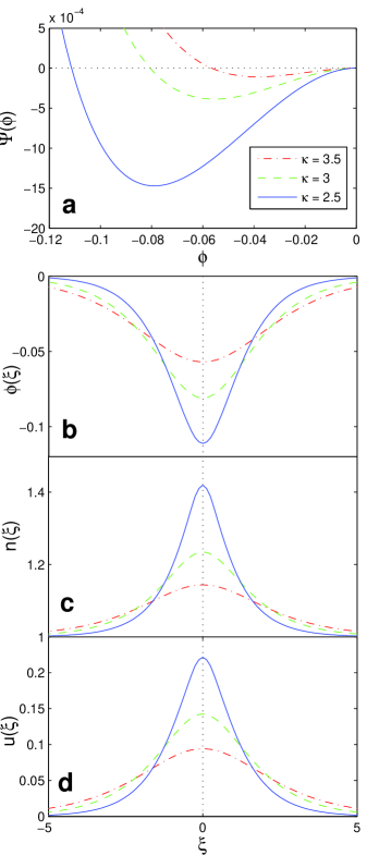
Figure 5: (Color online) (a) The pseudopotential $\Psi(\phi)$ and the associated solutions: (b) electric potential pulse $\phi$, (c) density $n$, and (d) velocity $u$ are depicted versus position $\xi$, for different $\kappa$. We have taken: $\kappa=2.5$ (solid curve), $3$ (dashed curve), and $3.5$ (dot-dashed curve). The other parameter values are: $\sigma=0.02$, $\beta=1.6$, and $M=0.75$.

Figure 3 shows the range of allowed Mach numbers as a function of $\kappa$, for various values of the temperature ratio $\sigma$. As discussed above, increasing $\kappa$ towards a Maxwellian distribution ($\kappa\rightarrow\infty$) broadens the Mach number range and yields higher values of Mach number. On the other hand, both upper and lower limits decrease as the limiting value $\kappa\rightarrow 3/2$ is approached. The qualitative conclusion is analogous to the trend in Fig. 2: stronger excess suprathermality leads to solitons occurring in narrower ranges of $M$. Furthermore, as illustrated in Figs. 2 and 3a, the Mach number threshold $M_{1}$ approaches the upper limit $M_{2}$ for high values of $\sigma$ and $\beta$: both increased hot-electron density and cool-electron thermal effects shrink the permitted soliton existence region.

Figure 3b depicts the range of allowed Mach numbers as a function of $\kappa$ for various values of the density parameter $\beta$ (for a fixed indicative $\sigma$ value). We note that both curves decrease with an increase in $\beta$. Although it lies in the damped region, we have also depicted a high $\beta$ regime for comparison (solid-crosses curve).

We conclude this section with a brief comparison of our work with that of Ref. Sahu2010, . The latter did not consider existence domains at all, let alone their dependence on plasma parameters, but merely plotted some Sagdeev potentials and associated soliton potential profiles for chosen values of some of the parameters, so as to extract some trends. En passant, there is indirect mention of an upper limit in $M$, in that it is commented that as increasing values of $M$ are considered, at some stage solitary waves cease to exist. Sahu2010

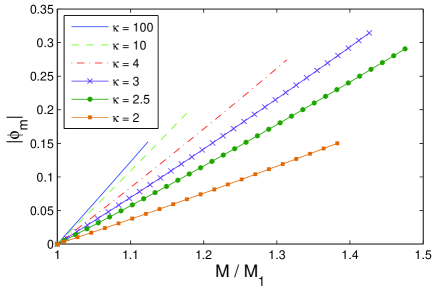
Figure 6: (Color online) The dependence of the pulse amplitude $|\phi_{m}|$ on the Mach number-to-sound-speed ratio $M/M_{1}$ is depicted, for different values of $\kappa$. From top to bottom: $\kappa=100$ (solid curve); $10$ (dashed curve); $4$ (dot-dashed curve); $3$ (crosses); $2.5$ (solid circles); $2$ (solid squares). Here, $\sigma=0.01$ and $\beta=1.3$.

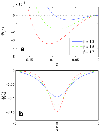
Figure 7: (Color online) (Upper panel) The pseudopotential $\Psi(\phi)$ vs. $\phi$ and (lower panel) the associated electric potential pulse $\phi$ vs. $\xi$ are depicted, for different values of the hot-to-cold electron density ratio $\beta$. From top to bottom: $\beta=1.3$ (solid curve); $1.5$ (dashed curve); $1.7$ (dot-dashed curve). Here $\sigma=0.01$, $\kappa=2.5$ and $M=0.75$.

VI Soliton characteristics

Having explored the existence domains of electron-acoustic solitons, subject to the constraints of the plasma model, we now turn to consider aspects of the soliton characteristics. We have numerically solved Eq. (32) for different representative parameter values, in order to investigate their effects on the soliton characteristics. We point out that, varying different parameters, we have found only negative potential solitons, regardless of the value of $\kappa$ considered. This is not altogether unexpected, as it has been found in a number of examples that, in contrast to the Cairns model, Cairns1995 , the kappa distribution does not lead to reverse polarity acoustic solitons. Baluku2008 ; Saini2009

Figure 4 shows the variation of the Sagdeev pseudopotential $\Psi(\phi)$ with the normalized potential $\phi$, along with the associated pulse solutions (soliton profiles), for different values of the temperature ratio, $\sigma=T_{c}/T_{h}$ (keeping $\beta=1.3$, $\kappa=2.5$ and Mach number $M=0.75$, all fixed). The Sagdeev potential well becomes deeper and wider as $\sigma$ is increased. We thus find associated increases in the soliton amplitude and in profile steepness (see Fig. 4b). Thermal effects therefore are seen to amplify significantly the electric potential disturbance at fixed $M$.

Figure 5a shows the Sagdeev pseudopotential $\Psi(\phi)$ for different values of $\kappa$. The electrostatic pulse (soliton) solution depicted in Fig. 5b is obtained via numerical integration. The pulse amplitude $|\phi_{\mathrm{m}}|$ increases for lower $\kappa$, implying an amplification of the electric potential disturbance as one departs from the Maxwellian. Once the electric potential has been obtained numerically, the cool-electron fluid density (Fig. 5c) and velocity disturbances (Fig. 5d) are determined algebraically. Both these disturbances are positive in this case, and again, for lower $\kappa$ values, the profiles reflecting the compression and the increase in velocity are steeper but narrower.

We recall that as various parameter values are varied, the true acoustic speed in the plasma configuration, $M_{1}$, also varies. As solitons are inherently super-acoustic, it is clear that the effect of a changing true acoustic speed could mask other dependences. Hence it is also desirable to explore soliton characteristics as a function of the propagation speed $M$, measured relative to the true acoustic speed, $M_{1}$. This ratio, $M/M_{1}$, thus represents the “true” Mach number. It has been shown that for any plasma made up of barotropic fluids, arbitrary amplitude solitons satisfy $\partial\Psi/\partial M<0$, Verheest2010 ; Verheest2010a ; Verheest2010b from which it follows that $\partial\phi_{m}/\partial M>0$, where $\phi_{m}$ is the soliton amplitude. Thus one expects that the soliton amplitude is an increasing function of $M/M_{1}$. This is true for both KdV solitons (small amplitudes, propagating near the sound speed) – “taller is faster”– and, in principle, also for fully nonlinear (Sagdeev) pulses (where the soliton characteristics can only be found numerically. Saini2009 ; Baluku2010a ) In Fig. 6, we have plotted the soliton amplitude $|\phi_{\mathrm{m}}|$ as a function of the ratio $M/M_{1}$, for a range of values of the parameter $\kappa$. Clearly, the amplitude increases linearly with $M/M_{1}$ for all values of $\kappa$. The two plots for $\kappa\leq 2.5$ both cover the full range up to $M=M_{2}$. However, although we deduce from earlier figures that $M_{2}$ increases with $\kappa$, we see that the endpoints of the plots for $\kappa\geq 3$ occur at decreasing values of $M/M_{1}$, and indeed decreasing maximum amplitudes $\phi_{m}$. That occurs as, for the chosen values of $\beta$ and $\sigma$, $M_{2}$ exceeds unity for $\kappa\geq 3$, and we have truncated the curves at the point where $M=1$, to remain within the range defined by the plasma model.

The effect of the hot-to-cool electron density ratio, $\beta$ on the soliton characteristics is shown in Fig. 7. We see that the soliton excitations are amplified and profiles steepened (the Sagdeev potential well becomes wider and deeper), as the density of the hot (nonthermal) electrons is increased (i.e., for higher $\beta$), viz., keeping $\kappa$, $\sigma$ and $M$ fixed. Furthermore, an increase in the number density of the hot electrons also leads to an increase in the perturbation of both density $n$, and velocity $u$ of the cool electrons (figure omitted).

VII Conclusion

In this article, we have performed a thorough linear and nonlinear analysis, from first principles, of electron acoustic excitations occurring in a nonthermal plasma consisting of hot $\kappa$-distributed electrons, adiabatic cool electrons, and immobile ions.

First, we have derived a linear dispersion relation, and investigated the dependence of the dispersion characteristics on the plasma environment (degree of ‘suprathermality’ through the parameter $\kappa$, plasma composition, and thermal effects).

Then, we have employed the Sagdeev pseudopotential method to investigate large amplitude localized nonlinear electrostatic structures (solitary waves), and to determine the region in parameter space where stationary profile solutions may exist. Only negative potential solitons were found. The existence domain for solitons was shown to become narrower in the range of solitary wave speed, with an increase in the excess of suprathermal electrons in the hot electron distribution (stronger ‘suprathermality’, lower $\kappa$ value). The dependence of the soliton characteristics on the hot electron number density (through the parameter $\beta$) and on the hot-to-cool electron temperature ratio $\sigma$, were also studied. A series of appropriate examples of pseudopotential curves and soliton profiles were computed numerically, in order to confirm the predictions arising from the study of existence domains.

It may be added that ionic motion/inertia, here neglected, may also be included for a more accurate description, but is likely to have only minor quantitative effects.

We note, for completeness, that very recently two related papers have appeared with a scope apparently similar to that of the present article, viz., Refs. Younsi2010 ; Sahu2010 . A word of comparison may therefore be appropriate here, for clarity. The latter authors Younsi2010 indicate that they are using a form of kappa distribution from one of the pioneering papers in the field. Thorne1991 Unfortunately, their expression for the characteristic speed $\theta$ does not agree with the standard expression Thorne1991 , and thus the hot electron density does not take the usual form, Eq. (5). Baluku2008 Further, they use values of $\kappa\geq 0.6$, i.e., well below the standard $\kappa$-distribution cut-off of 3/2. Hence their results do not apply to the standard form of $\kappa$ distribution. Hellberg2009

As regards the other paper, Sahu2010 it did not consider existence domains at all (apart from an indirect mention of an upper limit in $M$, as commented on in Section V above). Further, no account is taken in the paper of the possible effects of Landau damping on sustainable nonlinear structures, and a number of the figures relate to values of $\beta$ (called $\alpha$ in the paper) which lie in the unphysical, damped range.

We note that Ref. Sahu2010, has also carried out a “small amplitude” calculation yielding double layers. However, when evaluated numerically, these turn out to be well beyond the range of small amplitude, and that raises some doubts about the validity of the results (their Figures 8-10). Further, let us take together their Figures 2 and 8, and consider the case of $\kappa=3$ and $\alpha=0.2$ (i.e., our $\beta$). The latter is, of course, a value for which the linear wave is likely to be strongly Landau damped. It appears from the figures that a soliton occurs at $M=1.1$ with amplitude $\sim 0.9$, while a double layer occurs for $M=2.0$ with amplitude $\sim 0.7$. This combination of data does not satisfy the analytically-proven requirement that $\partial\Psi/\partial M<0$, Verheest2010 ; Verheest2010a ; Verheest2010b . There is no obvious reason why that should be the case, and there thus seems to be an error in at least one of these two figures.

Finally, we point out that we have not sought double layers in our calculations. However, we would be surprised if they did occur, as they are usually found as the upper limit to a sequence of solitons for a polarity for which there is no other limit. In this case there clearly is an upper limit for negative solitary waves, arising from the constraint $F_{2}(M)=0$. It is in principle possible for a double layer to occur at a lower value of $M$, and be followed by larger amplitude solitons at higher $M$, until the upper fluid cutoff such as a sonic point or an infinite compression cutoff is reached. Baluku2010 However, such behaviour depends on the the Sagdeev potential having a fairly complicated shape, with subsidiary local maxima, and we have not observed these for this model.

We are not aware of any experimental studies with which these theoretical results may be directly compared. However, it has previously been shown that wave data may be used to obtain an estimate for $\kappa$, thus acting as a diagnostic for the distribution function Hellberg2000 ; Vinas2005 .

Similarly, in this case there are a number of indicators amongst our results which experimenters may wish to consider when interpreting observations. Thus, for instance, a lower normalized phase velocity of the linear electron-acoustic wave than would be predicted by a Maxwellian model (see Fig. 1) could be used to evaluate $\kappa$.

Secondly, from Fig. 2 one sees that in low-$\kappa$ plasmas the range of normalized soliton speeds is both narrower and of larger value than one would expect for a Maxwellian. Thus, if solitons are found with normalized speeds around $M\simeq 0.4$, these can be understood only by allowing for additional suprathermal electrons (lower $\kappa$). Further, from Fig. 2 it follows that Maxwellian electrons give rise to a cutoff in the density ratio $\beta\simeq 1$, and hence solitons observed in such plasmas can only be explained in terms of lower $\kappa$.

From Fig. 5 we note that at fixed values of the normalized soliton speed, $M$, the amplitudes of the perturbations of the normalized potential, cool electron density and cool electron speed due to the solitary waves all increase with decreasing $\kappa$. This is related to the increase of the true Mach number $M/M_{1}$ for smaller $\kappa$, as the phase velocity $M_{1}$ is decreased. Thus larger disturbances are likely to be associated with increased suprathermality.

Finally, turning to Fig. 6, two effects are observed: At fixed true Mach number, $M/M_{1}$, the soliton amplitude decreases with decreasing $\kappa$ (increasing suprathermality). Despite that, the maximum values of soliton amplitude is found to occur not for a Maxwellian, but for the relatively low-$\kappa$ values of around 2.5-3. Thus, again, large observed amplitudes are likely to be associated with a low-$\kappa$ plasma.

Hence, as shown above, these results could assist in the understanding of solitary waves observed in two-temperature space plasmas, which are often characterized by a suprathermal electron distribution.

References

- (1) R. L. Tokar and S. P. Gary, Geophys. Res. Lett. 11, 1180 (1984).
- (2) S. P. Gary and R. L. Tokar, Phys. Fluids 28, 2439 (1985).
- (3) R. L. Mace and M. A. Hellberg, J. Plasma Phys. 43, 239 (1990).
- (4) M. Berthomier, R. Pottelette, and R. A. Treumann, Phys. Plasmas 6, 467 (1999).
- (5) R. L. Mace, G. Amery, and M. A. Hellberg, Phys. Plasmas 6, 44 (1999).
- (6) D. Henry and J. P. Treguier, J. Plasma Phys. 8, 311 (1972).
- (7) S. Ikezawa and Y. Nakamura, J. Phys. Soc. Jpn. 50, 962 (1981).
- (8) M. F. Thomsen, H. C. Barr, S. P. Gary, W. C. Feldman, and T. E. Cole, J. Geophys. Res. 88, 3035 (1983).
- (9) W. C. Feldman, R. C. Anderson, S. J. Bame, et al., J. Geophys. Res. 88, 96 (1983).
- (10) S. D. Bale, P. J. Kellogg, D. E. Larson, R. P. Lin, K. Goetz, and R. P. Lepping, Geophys. Res. Lett. 25, 2929 (1998).
- (11) C. S. Lin, J. L. Burch, S. D. Shawhan, and D. A. Gurnett, J. Geophys. Res. 89, 925 (1984).
- (12) H. Matsumoto, H. Kojima, T. Miyatake, et al., Geophys. Res. Lett. 21, 2915 (1994).
- (13) C. A. Cattell, J. Dombeck, J. R. Wygantet, et al., Geophys. Res. Lett. 26, 425 (1999).
- (14) A. P. Kakad, S. V. Singh, R. V. Reddy, G. S. Lakhina, and S.G. Tagare, Adv. Space Res. 43, 1945 (2009).
- (15) K. Watanabe and T. Taniuti, J. Phys. Soc. Jpn. 43, 1819 (1977).
- (16) K. Nishihara and M. Tajiri, J. Phys. Soc. Jpn. 50, 4047 (1981).
- (17) M. Berthomier, R. Pottelette, and M. Malingre, J. Geophys. Res. 103, 4261 (1998).
- (18) D. Summers and R. M. Thorne, Phys. Fluids B 3, 1835 (1991)
- (19) M. A. Hellberg, R. L. Mace, R. J. Armstrong, and G.Karlstad, J. Plasma Phys. 64, 433 (2000).
- (20) T. K. Baluku and M. A. Hellberg, Phys. Plasmas 15, 123705 (2008).
- (21) V. Pierrard and M. Lazar, Solar Phys. 267, 153 (2010).
- (22) M. A. Hellberg, R. L. Mace, T. K. Baluku, I. Kourakis and N. S. Saini, Phys. Plasmas 16, 094701 (2009).
- (23) V. M. Vasyliunas, J. Geophys. Res. 73, 2839 (1968).
- (24) S. P. Christon, D. G. Mitchell, D. J. Williams, et al., J. Geophys. Res. 93, 2562 (1988).
- (25) V. Pierrard and J. F. Lemaire, J. Geophys. Res. 101, 7923 (1996).
- (26) P. Schippers, M. Blanc, N. André, I. Dandouras, G. R. Lewis, L. K. Gilbert, A. M. Persoon, N. Krupp, D. A. Gurnett, A. J. Coates, S. M. Krimigis, D. T. Young, and M. K. Dougherty, J. Geophysical Research, 113, A07208 (2008).
- (27) B. D. Fried and R. W. Gould, Phys. Fluids 4, 139 (1961).
- (28) M. A. Hellberg and R. L. Mace, Phys. Plasmas 9, 1495 (2002).
- (29) T. K. Baluku, M. A. Hellberg, and R. L. Mace, J.Geophys. Res. 116, A04227 (2011).
- (30) N. Dubouloz, R. Pottelette, M. Malingre, and R. A. Treumann, Geophys. Res. Lett. 18, 155 (1991).
- (31) S. V. Singh and G. S. Lakhina, Nonlin. Proc. Geophys. 11, 275 (2004).
- (32) T. Cattaert, F. Verheest, and M. A. Hellberg, Phys. Plasmas 12, 042901 (2005).
- (33) F. Verheest, T. Cattaert, and M. A. Hellberg, Space Sci. Rev. 121, 299 (2005).
- (34) I. Kourakis and P. K. Shukla, Phys. Rev. E 69, 036411 (2004).
- (35) S. Sultana, I. Kourakis, N. S. Saini and M.A. Hellberg, Phys. Plasmas 17, 032310 (2010).
- (36) M. Berthomier, R. Pottelette, M. Malingre, and Y. Khotyaintsev, Phys. Plasmas 7, 2987 (2000).
- (37) R. L. Mace and M. A. Hellberg, Phys. Plasmas, 8, 2649 (2001).
- (38) S. Sultana and I. Kourakis, Plasma Phys. Control. Fusion 53, 045003 (2011).
- (39) B. Sahu, Phys. Plasmas 17, 122305 (2010)
- (40) Y. F. Chateau, N Meyer-Vernet, J. Geophys. Res. 96, 5825 (1991).
- (41) D. A. Bryant, J. Plasma Phys. 56, 87 (1996).
- (42) R. L. Mace, M. A. Hellberg, and R. A. Treumann, J. Plasma Phys. 59, 393 (1998).
- (43) F. Verheest, T. Cattaert, G. S. Lakhina, and S. V. Singh, J. Plasma Phys. 70, 237 (2004).
- (44) J. F. McKenzie, E. Dubinin, K. Sauer, and T. B. Doyle, J. Plasma Phys. 70, 431 (2004).
- (45) F. Verheest, M. A. Hellberg, and G. S. Lakhina, Astrophys. Space Sci. Trans. 3, 15 (2007).
- (46) R. A. Cairns, A. A. Mamun, R. Bingham, R. Boström, R. O. Dendy, C. M. C. Nairn, and P. K. Shukla, Geophys. Res. Lett. 22, 2709 (1995).
- (47) N. S. Saini, I. Kourakis, and M. A. Hellberg, Phys. Plasmas 16, 062903 (2009).
- (48) F. Verheest Phys. Plasmas 17, 062302 (2010).
- (49) F. Verheest and M. A. Hellberg, Phys. Plasmas 17, 023701 (2010).
- (50) F. Verheest and M. A. Hellberg, J. Plasma Phys. 76, 277 (2010).
- (51) T. K. Baluku, M. A. Hellberg, N. S. Saini and I. Kourakis, Phys. Plasmas, 17, 053702 (2010).
- (52) S. Younsi and M. Tribeche, Astrophys. Space Sci. 300, 295 (2010).
- (53) R. M. Thorne and D. Summers, Phys. Fluids B 3, 2117 (1991).
- (54) T. K. Baluku, M. A. Hellberg and F. Verheest, EuroPhysics Letters 91, 15001 (2010).
- (55) A.F. Viñas, R.L. Mace and R.F. Benson, J. Geophys. Res. 110, A06202 (2005).