Realistic extensions of a Brownian ratchet for protein translocation

Abstract

We study a model for the translocation of proteins across membranes through a nanopore using a ratcheting mechanism. When the protein enters the nanopore it diffuses in and out of the pore according to a Brownian motion. Moreover, it is bound by ratcheting molecules which hinder the diffusion of the protein out of the nanopore, i.e. the Brownian motion is reflected such that no ratcheting molecule exits the pore. New ratcheting molecules bind at rate $\gamma$. Extending our previous approach (Depperschmidt and Pfaffelhuber, 2010) we allow the ratcheting molecules to dissociate (at rate $\delta$) from the protein (Model I). We also provide an approximate model (Model II) which assumes a Poisson equilibrium of ratcheting molecules on one side of the current reflection boundary. Using analytical methods and simulations we show that the speed of both models are approximately the same. Our analytical results on Model II give the speed of translocation by means of a solution of an ordinary differential equation.

1 Introduction

Most proteins are generated within the cellular cytosol and have to be transported where they are needed. Frequently, they have to be transported across membranes, e.g. into the endoplasmatic reticulum, mitochondria or other organelles, or they are secreted, i.e. transported across the cell wall (Neupert and Brunner, 2002). Protein translocation occurs either co-translationally, e.g. when ribosomes attach to the membrane of the endoplasmatic reticulum and proteins are transported into the lumen through a nanopore already during translation, or post-translationally (Rapoport, 2007).

Consider translocation into mitochondria first. Over 99% of mitochondrial proteins are translocated post-translationally (Wickner and Schekman, 2005) and the molecular mechanisms have been studied in detail. When a substrate is translocated into the mitochondrium, it has to cross the translocase outer membrane (TOM) and the translocase inner membrane (TIM). The mitochondrial heat shock protein 70 (mtHsp70) is known to play a crucial role in translocation of substrates (Glick, 1995). mtHsp70 changes between its ATP-bound form, where it has an open pocket for binding to the substrate, and the ADP-bound form where the pocket is closed (Neupert and Brunner, 2002; Neupert and Herrmann, 2007). There are two differing opinions about the role of mtHsp70 in translocation. Either mtHsp70 pulls actively the substrate through the nanopore, or it only prevents backsliding of the substrate, leading to a passive mechanism (Glick, 1995; Neupert and Brunner, 2002; Neupert and Herrmann, 2007). Such a ratcheting mechanism was first introduced by Schneider et al (1994) and Okamoto et al (2002). The best argument for active pulling is that the protein which is translocated must be unfolded outside the mitochondria, so translocation occurs against a force (Pfanner and Truscott, 2002). However, experimental evidence is still lacking and binding of mtHsp70 to the substrate can explain observations (Neupert and Herrmann, 2007).

Many proteins are translocated into the endoplasmatic reticulum already during translation. Moreover, post-translational translocation has been suggested to occur through a passive ratcheting mechanism in eukaryotic cells by Matlack et al (1999). Here, the nanopore is formed by the Sec63 complex and the ratcheting molecules are called BiP which is a member of the Hsp70 family. BiP exists in an ATP-bound state with an open binding pocket. This is activated by an interaction with the J-domain of Sec63, which can also close the binding pocket after BiP is bound to the substrate. Interestingly, BiP binds unspecifically to the substrate and therefore is able to mediate translocation of many different proteins (Rapoport, 2007). For protein translocation into chloroplasts in plants, ratcheting mechanisms have not yet been considered yet (Strittmatter et al, 2010; Li and Chiu, 2010).

Quantitative descriptions of cellular ratcheting mechanisms began with pioneering work of Simon et al (1992) and Peskin et al (1993). In their model, ratcheting molecules can bind to the protein at the nanopore and hinder diffusion out of the nanopore completely (perfect ratchet) or only with a probability $p<1$ (imperfect ratchet). The assumption that ratcheting molecules can only bind directly at the pore is motivated by translocation into the endoplasmatic reticulum where the ratcheting molecule, BiP, is known to interact with Sec61 which builds the pore. However, the interaction with the nanopore can only mean that concentration of ratcheting molecules is higher near the pore. (See Griesemer et al (2007), for a mathematical model of the interaction of the ratcheting molecule with the nanopore.) We take the same approach as D’Orsogna et al (2007) and assume that ratcheting molecules may bind uniformly along the protein. This assumes that the concentration of ratcheting molecules is approximately constant between the pore and the first bound molecules.

Most quantitative descriptions of the Brownian ratchet assume a finite length of ratcheting molecules (e.g. Zandi et al, 2003; D’Orsogna et al, 2007). Ambjornsson et al (1992) describe a car parking effect arising by the distribution of ratcheting molecules along the substrate. They assume a fast binding and unbinding of ratcheting molecules, leading to an effective probability any position of the protein is bound. The case of fast binding is studied in Budhiraja and Fricks (2006), who derive a law of large numbers and a central limit theorem in the case that Brownian motion has a drift. Effects of binding affinities which depend on the protein sequence have been put forward in Abdolvahab et al (2008, 2011).

The goal of this paper is to introduce a realistic model for the ratcheting mechanism for protein translocation in mitochondria and the endoplasmatic reticulum as described above. Elston (2002) tried to decide if translocation happens actively (by pulling the protein) or passively (by a ratcheting mechanism) using likelihood ratio tests. However, after fitting the model parameters using least squares, their statistical tests were not significant and both models fitted experimental data well. New molecular techniques have to give rise to better data to decide between active an passive transport. In the present paper, we obtain predictions for the speed of translocation which will shed light on empirical studies in the future.

Our model of the Brownian ratchet is similar to the ratchet studied in Liebermeister et al (2001), but is continuous, assumes free diffusion of the protein and binding of ratcheting molecules anywhere along the protein. Since ratcheting molecules can dissociate from the protein, we call the process a broken Brownian ratchet. We give two models, termed Model I and Model II. For Model I, which takes into account every ratcheting molecule at all times, we can only show that the speed of translocation is positive (Theorem 2.1). Model II serves as an approximation. When a ratcheting molecule dissociates, we assume that binding and unbinding of ratcheting molecules is in equilibrium. This model is easier to analyze but has about the same behavior for the speed of translocation (see the simulation results in Figure 3). For Model II, we can show a law of large numbers giving the speed of transport in terms of a solution of a differential equation, Theorem 2.2.

2 The model

The model we study extends the Brownian ratchet introduced in Depperschmidt and Pfaffelhuber (2010). Namely, protein translocation across a membrane is based on the following assumptions:

1. The protein moves in and out with the same probability.

2. The protein movement is reflected at binding ratcheting molecules.

3. The protein is infinitely long.

4. The ratcheting molecules are infinitely small.

5. Ratcheting molecules may bind to the protein at a continuum of sites.

6. The ratcheting molecules may dissociate from the protein.

These assumptions are exactly the same as in Depperschmidt and Pfaffelhuber (2010) except for the last. They assumed that the dissociation rate of the ratcheting molecules from the protein is much smaller than their binding rate to the protein, leading to effectively no dissociation of ratcheting molecules.

First, we translate the above set of assumptions into a mathematical model. By $X_{t}$, we denote the total length of the protein which already crossed the membrane between times $0$ and $t$. In addition, $R_{t}\leq X_{t}$ is the largest distance of $X_{t}$ to a ratcheting molecule. We assume that the protein has already moved across the membrane by time $0$, such that ratcheting molecules may bind between $X_{t}$ and $-\infty$ at constant rate. Consider the pair $(X_{t},R_{t})_{t\geq 0}$, where $(X_{t})_{t\geq 0}$ is a Brownian motion, started in $X_{0}=x$, reflected at $R_{t}:=\sup\mathcal{R}_{t}$ and $\mathcal{R}_{t}\subseteq(-\infty,X_{t}]$ is the random set of all bound ratcheting molecules at time $t$. The dynamics of $\mathcal{R}_{t}$ is as follows: starting in $\mathcal{R}_{0}=\{0\}$, a point at $dx$ is added at rate $\gamma{\mathds{1}}_{x\in(-\infty,X_{t}]}dx$ (i.e. a transition from $\mathcal{R}_{t-}$ to $\mathcal{R}_{t}:=\mathcal{R}_{t-}\cup\{x\}$ occurs). In addition, every $x\in\mathcal{R}_{t}$ is deleted at rate $\delta$ (i.e. a transition from $\mathcal{R}_{t-}$ to $\mathcal{R}_{t}:=\mathcal{R}_{t-}\setminus\{x\}$ occurs at rate $\delta{\mathds{1}}_{x\in\mathcal{R}_{t-}}$). Note that the last mechanism with rate $\delta$ models the dissociation of ratcheting molecules from the protein (see (vi) above). We rely on the following graphical construction, which is illustrated in Figure 1.

Definition 1 ($\gamma/\delta$-broken Brownian ratchet, Model I)

Let $\mathcal{N}^{\gamma,\delta}$ be a Poisson point process on $[0,\infty)\times\mathbb{R}\times[0,\infty)$ with intensity measure $\gamma\delta e^{-\delta z}\lambda^{3}(d\tau,dr,dz)$, conditioned on $\mathcal{N}^{\gamma,\delta}(\{0\}\times\{0\}\times[0,\infty))=1$, where $\gamma>0,\delta\geq 0$ and $\lambda^{3}$ denotes the Lebesgue measure on $[0,\infty)\times\mathbb{R}\times[0,\infty)$. Moreover, $\mathcal{N}^{\gamma}$ is the projection of $\mathcal{N}^{\gamma,\delta}$ on the first two coordinates. Let $(B_{t}^{0})_{t\geq 0},(B_{t}^{1})_{t\geq 0},\dots$ be a sequence of independent Brownian motions, independent of $\mathcal{N}^{\gamma,\delta}$, with $B_{0}^{0}=B_{0}^{1}=\cdots=0$. We define recursively times $t_{0},t_{1},\dots$ when the reflection boundary changes as well as triples $(\tau_{0},r_{0},z_{0}),(\tau_{1},r_{1},z_{1}),(\tau_{2},r_{2},z_{2}),\dots\in\mathcal{N}^{\gamma,\delta}$ such that $r_{n}$ is the reflection boundary in the interval $[t_{n},t_{n+1})$. Define $t_{0}=\tau_{0}=r_{0}=0$, $z_{0}:=z$ if $(0,0,z)\in\mathcal{N}^{\gamma,\delta}$ and for $x_{0}\geq 0$ set $X_{t}:=|x_{0}+B_{t}^{0}|$ for $t_{0}\leq t<t_{1}$, and the set of new reflection boundaries above $r_{n}$ before time $\tau_{n}+z_{n}$,

$$\Gamma_{n} :=\{(\tau,r,z)\in\mathcal{N}^{\gamma,\delta}:t_{n}\leq\tau<\tau_{n}+z_{n},r_{n}\leq r<X_{\tau}\},$$ (2.1)

$$\inf\Gamma_{n} :=(\tau,r,z)\text{ if }(\tau,r,z)\in\Gamma_{n}\text{ and }\tau=\inf\pi_{1}\Gamma_{n},$$

where $\pi_{1}$ is the projection on the first coordinate. Now, we set recursively for $n=0,1,2,\dots$

$$t_{n+1} :=(\tau_{n}+z_{n})\wedge\inf\pi_{1}\Gamma_{n},$$ (2.2)

$$(\tau_{n+1}, \,r_{n+1},z_{n+1}):=\begin{cases}\inf\Gamma_{n},&\text{ if }\Gamma_{n}\not=\emptyset,\\[4.30554pt] (\tau,r,z)&\text{ if }\Gamma_{n}=\emptyset\text{ and }\\ &\quad r=\max\{r\leq X_{\tau}:\tau\leq\tau_{n}+z_{n}<\tau+z\}.\end{cases}$$

Finally,

$$\left.\begin{aligned} R_{t}&:=r_{n},\\ X_{t}&:=R_{t}+|B_{t-t_{n}}^{n}+X_{t_{n}-}-R_{t}|\end{aligned}\right\}\text{ for $t_{n}\leq t<t_{n+1}$.}$$ (2.3)

We refer to the process $(X_{t},R_{t})_{t\geq 0}$ as the $\gamma/\delta$-broken Brownian ratchet, Model I with initial value $(X_{0},R_{0})=(x_{0},0)$.

Remark 1 (Interpretation)

In the definition above, $(\tau,r,z)\in\mathcal{N}^{\gamma,\delta}$ represents a ratcheting molecule which binds at time $\tau$ at position $r$ to the protein and stays bound up to time $\tau+z$. We start at time $t=0$ with one bound molecule at position 0. The variables $t_{1},t_{2},\dots$ represent times when the reflection boundary changes. Note that $R_{t}$, at any time $t$, is the position of the ratcheting molecule which is bound (i.e. $\tau\leq t<\tau+z$) and closest to $X_{t}$. By time $t$, let us denote by $(\tau,r,z)\in\mathcal{N}^{\gamma,\delta}$ the active point if $R_{t}=r$ (and recall that all points in $\mathcal{N}^{\gamma,\delta}$ have all coordinates different, almost surely). By definition, $t_{n}$ is the time when the active point changes for the $n$th time. There are two possibilities when the active point $(\tau,r,z)$ changes. First, a new Poisson point can fall between $r$ and $X_{t}$ (as described by the first line in (2.2)). Second, when $t=\tau+z$, the current active point dissociates, and the next active point is the one closest to $X_{t}$ (given by the second line in (2.2)). Last, note that $X_{t_{n}}=X_{t_{n}-}$ by construction, for all $n$, meaning that $(X_{t})_{t\geq 0}$ is continuous and note that $|B_{t-t_{n}}^{k}+X_{t_{n}-}-R_{t}|$ is a Brownian motion, started at $X_{t_{n}-}-R_{t}$, reflected at 0, such that $(X_{t})_{t\geq 0}$ is reflected at $R_{t}$ at all times.

The graphical construction of $(X_{t})_{t\geq 0}$ is done step by step between jump times of the reflection boundary, $(R_{t})_{t\geq 0}$, i.e. when the active point changes. This works since, after any finite time $t$ there may only be a finite number of jumps of the reflection boundary so that the construction works for any large time.

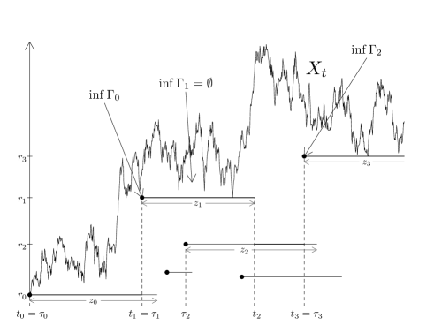
Figure 1: One realization of the graphical construction of Model I. The path of $(X_{t})_{t\geq 0}$ is reflected at the boundary $(R_{t})_{t\geq 0}$.

For Model I we show the following result.

Theorem 2.1 (Speed of the broken Brownian ratchet, Model I)

Let $(X_{t},R_{t})_{t\geq 0}$ be a broken Brownian ratchet, Model I. Then, there are constants $0<c\leq C<\infty$, where $c$ depends on $\gamma$ and $\delta$ and $C$ only depends on $\gamma$ such that

$$c\leq\underline{a}_{\gamma,\delta}:=\liminf_{t\to\infty}\frac{X_{t}}{t}\leq\overline{a}_{\gamma,\delta}:=\limsup_{t\to\infty}\frac{X_{t}}{t}\leq C$$

almost surely. Moreover, $\underline{a}_{\gamma,\delta}=\gamma^{1/3}\underline{a}_{1,\delta/\gamma^{2/3}}$ and $\overline{a}_{\gamma,\delta}=\gamma^{1/3}\overline{a}_{1,\delta/\gamma^{2/3}}$.

Remark 2 (Interpretation)

The result says that the speed of the broken Brownian ratchet, Model I, (if it exists as $a_{\gamma,\delta}:=\underline{a}_{\gamma,\delta}=\overline{a}_{\gamma,\delta}$) is positive, no matter how large $\delta$ is. In addition, it scales with $\gamma^{1/3}$ like $a_{\gamma,\delta}=\gamma^{1/3}a_{1,\delta/\gamma^{2/3}}$.

Although the speed of the broken Brownian ratchet is positive by Theorem 2.1, we aim at a more complete picture. However, the difficulty in the analysis of Model I is that it is not local in the sense that a single Poisson point can be active more than once. In particular, dependencies between Poisson points arise as time evolves. For this reason, we consider a second model with similar properties as Model I. Briefly speaking, we introduce a Model II by assuming that the possible reflection boundaries below the currently active one are always in their equilibrium.

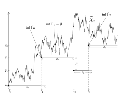
Figure 2: One realization of the graphical construction of Model II. The path of $(\widetilde{X}_{t})_{t\geq 0}$ is reflected at the boundary $(\widetilde{R}_{t})_{t\geq 0}$. Random variables $Z_{0},Z_{1},...$ are independent and Exp$(\delta)$-distributed, while $E_{0},E_{1},...$ are independent and Exp$(\gamma/\delta)$-distributed.

Remark 3 (Motivation)

Consider Model I and assume $(\tau,r,z)$ is the active point by time $t$. Consider a time $t^{\prime}>t$ when the active point changes and $t^{\prime}=\tau+z$. As an approximation, we assume that the set

$$\{r^{\prime}:(\tau^{\prime},r^{\prime},z^{\prime})\in\mathcal{N}^{\gamma,\delta}\text{ for some }\tau^{\prime},z^{\prime}\in[0,\infty),\tau^{\prime}\leq t^{\prime}\leq\tau^{\prime}+z^{\prime}\}$$

is in its stationary distribution which arises for $z\to\infty$, i.e. if the last active point stays for a long time. This stationary distribution is readily computed. It is clear that only points $r^{\prime}<r$ are possible. Moreover, the probability that a point in $dr^{\prime}$ is in the set equals

$$\int_{0}^{\infty}\gamma e^{-\delta z}dzdr^{\prime}=\frac{\gamma}{\delta}dr^{\prime}.$$

So, the set is distributed according to a Poisson process with intensity measure $\tfrac{\gamma}{\delta}{\mathds{1}}_{(-\infty,r]}(r^{\prime})\lambda(dr^{\prime})$. As a consequence, if the active point vanishes, the reflection boundary jumps down an exponentially distributed amount with rate $\gamma/\delta$ in the approximate model. This leads to the following Model II, which is illustrated in Figure 2.

Definition 2 ($\gamma/\delta$-Broken Brownian ratchet, Model II)

Let $\widetilde{\mathcal{N}}^{\gamma}$ be a Poisson point process on $[0,\infty)\times\mathbb{R}$ with intensity measure $\gamma\lambda^{2}(dt,dx)$, conditioned on $\widetilde{\mathcal{N}}^{\gamma}(\{0\}\times\{0\})=1$, where $\gamma>0$ and $\lambda^{2}$ denotes the Lebesgue measure on $[0,\infty)\times\mathbb{R}$. Moreover, $Z_{0},Z_{1},\dots$ are independent exponentially distributed with parameter $\delta\geq 0$ and $E_{0},E_{1},\dots$ are independent and exponentially distributed with parameter $\gamma/\delta$ (they are not needed if $\delta=0$). Let $(\widetilde{B}_{t}^{0})_{t\geq 0},(\widetilde{B}_{t}^{1})_{t\geq 0},\dots$ be a sequence of independent Brownian motions with $\widetilde{B}_{0}^{0}=\widetilde{B}_{0}^{1}=\dots=0$. Define $\widetilde{t}_{0}=\widetilde{r}_{0}=0$ and for $x_{0}\geq 0$ set $\widetilde{X}_{t}:=|x_{0}+\widetilde{B}_{t}^{0}|$ for $\widetilde{t}_{0}\leq t<\widetilde{t}_{1}$, and

$$\widetilde{\Gamma}_{n} :=\{(\tau,r)\in\widetilde{\mathcal{N}}^{\gamma}:\widetilde{t}_{n}\leq\tau<\widetilde{t}_{n}+Z_{n},r_{n}\leq r<X_{\tau}\},$$ (2.4)

$$\inf\widetilde{\Gamma}_{n} :=(\tau,r)\text{ if }(\tau,r)\in\Gamma_{n}\text{ and }\tau=\inf\pi_{1}\Gamma_{n},$$

where $\pi_{1}$ is the projection on the first coordinate. Now, we set recursively for $n=0,1,2,...$

$$\widetilde{t}_{n+1} :=(\widetilde{t}_{n}+Z_{n})\wedge\inf\pi_{1}\widetilde{\Gamma}_{n},$$ (2.5)

$$\widetilde{r}_{n+1} =\begin{cases}r&\text{ if }\widetilde{\Gamma}_{n}\neq\emptyset\text{ and }(\widetilde{t}_{n+1},r)=\inf\widetilde{\Gamma}_{n},\\ \widetilde{r}_{n}-E_{n},&\text{ if }\widetilde{\Gamma}_{n}=\emptyset.\end{cases}$$

Finally,

$$\left.\begin{aligned} \widetilde{R}_{t}&:=\widetilde{r}_{n},\\ \widetilde{X}_{t}&:=\widetilde{R}_{t}+|\widetilde{B}_{t-\widetilde{t}_{n}}^{k}+\widetilde{X}_{\widetilde{t}_{n}-}-\widetilde{R}_{t}|\end{aligned}\right\}\text{ for $\widetilde{t}_{n}\leq t<\widetilde{t}_{n+1}$.}$$ (2.6)

We refer to the process $(\widetilde{X}_{t},\widetilde{R}_{t})_{t\geq 0}$ as the $\gamma/\delta$-broken Brownian ratchet, Model II with initial value $(\widetilde{X}_{0},\widetilde{R}_{0})=(x_{0},0)$.

Theorem 2.2 (Speed of the broken Brownian ratchet, Model II)

Let $(\widetilde{X}_{t},\widetilde{R}_{t})_{t\geq 0}$ be a $\gamma/\delta$-broken Brownian ratchet, Model II. Then,

$$\lim_{t\to\infty}\frac{\widetilde{X}_{t}}{t}=-\frac{A^{\prime}(0)}{2A(0)}$$

almost surely, where $A$ is the first coordinate of a solution of the system

$$\begin{split}A^{\prime\prime}(z)&=-2\delta B(z)+2\gamma zA(z),\\ B^{\prime}(z)&=-A^{\prime}(z)-\frac{\gamma}{\delta}B(z)\end{split}$$ (2.7)

such that $A(0)=1/2$, $B(0)=0$ and $A$ is strictly decreasing with $A(z)\to 0$ as $z\to\infty$.

Remark 4 (Simulations, uniqueness of $A$, and the case $\delta=0$)

1. Since Model II is only a convenient approximation of Model I, we use simulations to see differences in the speed of Model I and II. By scaling properties of both models (see Propositions 1 and 3), we require simulations only for a single parameter $\gamma$. As can be seen in Figure 3, the speed of both models is almost the same. The fact that Model II is faster for low $\delta$ can be explained: we assume that the number of possible reflection boundaries below the currently active one is in equilibrium, which means that these are more than for Model I, where the equilibrium is not yet attained. Since more reflection boundaries mean that the broken Brownian ratchet moves faster, the speed of Model II is higher. For high values of $\delta$, Model I shows a higher speed in our simulations. The reason is that we fixed the reflection boundary at 0 in our simulations of Model I, and hence the simulations overstimate the speed of protein translocation.

2. For a proper use of Theorem 2.2 in Figure 3, we need to solve the system (2.7). We searched numerically for a solution by trying out various values for $A^{\prime}(0)$ and determined which value approximately leads to $A(z)\to 0$ as $z\to\infty$. In our numerical analysis, we found only a single value of $A^{\prime}(0)$ with this property, for all $\delta$. Hence, we strongly conjecture there is a unique solution of the system (2.7) satisfying $A(0)=1/2$, $B(0)=0$ and $A(z)\to 0$ as $z\to\infty$.

3. In the case $\delta=0$, the first equation in (2.7) reads $A^{\prime\prime}(z)-2\gamma zA(z)=0$. The only solution with the required boundary values is given by $z\mapsto Ai((2\gamma)^{1/3}z)/(2Ai(0))$, where $Ai$ is the Airy function (i.e. solution of $u^{\prime\prime}(z)-zu(z)=0$) going to 0 as $z\to\infty$. By well-known properties of $Ai$ (see e.g. Abramowitz and Stegun, 1972), the speed is thus given by

   $$\lim_{t\to\infty}\frac{X_{t}}{t} =-\frac{Ai^{\prime}(0)}{2Ai(0)}(2\gamma)^{1/3}=\frac{\Gamma(2/3)}{\Gamma(1/3)}\Big{(}\frac{3\gamma}{4}\Big{)}^{1/3}\approx 0.36\cdot(2\gamma)^{1/3},$$ (2.8)

   a result known from Theorem 1 in Depperschmidt and Pfaffelhuber (2010).

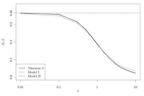
Figure 3: A simulation study for the speed of the broken Brownian ratchet, Model I and Model II. The parameter $\gamma=\tfrac{1}{2}$ is fixed. See also Remark 4. The horizontal line at 0.36 represents the speed in the case $\delta=0$ from (2.8).

3 Proofs: Model I

In this section, we prove Theorem 2.1. Three ingredients are needed: First, a scaling property for the $\gamma/\delta$-broken Brownian ratchet, Model I, is obtained in Section 3.1. Second, an upper bound for the speed can trivially be obtained by setting $\delta=0$ and using results from Depperschmidt and Pfaffelhuber (2010). Third, a lower bound is obtained by thinning Model I, which we do in Section 3.2. We conclude the proof in Section 3.3.

3.1 Scaling property

Here we obtain a scaling property of the $\gamma/\delta$-broken Brownian ratchet, Model I, which is based on a rescaling of space and time in Definition 1.

Proposition 1 (Scaling property, Model I)

Let $(X_{t}^{\gamma;\delta},{R}_{t}^{\gamma;\delta})_{t\geq 0}$ be the $\gamma/\delta$-broken Brownian ratchet, Model I, with $\gamma>0$, $\delta\geq 0$ and initial value $(0,0)$. Then

$$(X_{t}^{\gamma;\delta},R_{t}^{\gamma;\delta})_{t\geq 0}\overset{d}{=}\gamma^{-\frac{1}{3}}\left(X_{\gamma^{2/3}t}^{1;\delta/\gamma^{2/3}},R_{\gamma^{2/3}t}^{1;\delta/\gamma^{2/3}}\right)_{t\geq 0},$$ (3.1)

where   $\stackrel{{\scriptstyle d}}{{=}}$   denotes equality in distribution.

Proof

Using the notation from Definition 1, we need to understand what (3.1) means for the Poisson process $\mathcal{N}^{\gamma,\delta}$ and for the Brownian motions $(B_{t}^{0})_{t\geq 0},(B_{t}^{1})_{t\geq 0},\dots$ We use the linear rescaling of time and space

$$g_{\gamma}:\begin{cases}{\mathbb{R}}^{3}&\to{\mathbb{R}}^{3}\\ (t,x,z)&\mapsto(\gamma^{2/3}t,\gamma^{1/3}x,\gamma^{2/3}z).\end{cases}$$

and obtain $g_{\gamma}(\mathcal{N}^{\gamma,\delta})\stackrel{{\scriptstyle d}}{{=}}\mathcal{N}^{1,\delta/\gamma^{2/3}}$. Moreover, we have that $(\sqrt{c}B^{k}_{t})_{t\geq 0}\overset{d}{=}\big{(}B^{k}_{ct}\big{)}_{t\geq 0}$ for all $c>0$ and $k=0,1,2,\dots$ and so, if $\widetilde{g}_{\gamma}:\mathbb{R}^{2}\to\mathbb{R}^{2}$ consists of the first two coordinates of $g_{\gamma}$,

$$\widetilde{g}_{\gamma}\left((t,{B}_{t}^{k})_{t\geq 0}\right) =\left(\big{(}\gamma^{2/3}t,\gamma^{1/3}{B}_{t}^{k}\big{)}_{t\geq 0}\right)$$ (3.2)

$$\overset{d}{=}\left(\big{(}\gamma^{2/3}t,{B}^{k}_{\gamma^{2/3}t}\big{)}_{t\geq 0}\right)=\left(\big{(}s,B_{s}^{k}\big{)}_{s\geq 0}\right)$$

for $k=0,1,2,\dots$ where $s:=\gamma^{2/3}t$. Hence, the distribution of the Brownian motions are unaffected by the rescaling. We have shown that

$$\gamma^{1/3}(X_{t}^{\gamma,\delta},R_{t}^{\gamma,\delta})_{t\geq 0}\stackrel{{\scriptstyle d}}{{=}}(X_{\gamma^{2/3}t}^{1,\delta/\gamma^{2/3}},R_{\gamma^{2/3}t}^{1,\delta/\gamma^{2/3}})_{t\geq 0}$$

and the assertion follows. ∎

3.2 Lower bound

Consider the possible reflection boundaries $[\tau,\tau+z)\times\{r\}$ for all $(\tau,r,z)\in\mathcal{N}^{\gamma,\delta}$ in Definition 1. Clearly, the speed of the $\gamma/\delta$-ratchet decreases if we take less possible reflection boundaries, leading to a lower bound for the speed of the broken ratchet. We will use the following thinned version of Model I. Note that the formal difference to Model I is the restriction $\sup\Sigma_{n+1}\leq\tau$ in (3.4). An illustration can be found in Figure 4.

Definition 3 ($\gamma/\delta$-broken Brownian ratchet, thinned Model I)

Consider the same probability space as in Definition 1, with the same $\mathcal{N}^{\gamma,\delta},\mathcal{N}^{\gamma},(B_{t}^{0})_{t\geq 0},(B_{t}^{1})_{t\geq 0},(B_{t}^{2})_{t\geq 0},\dots$ Again, we define recursively times $\widehat{t}_{0},\widehat{t}_{1},\dots$ when the reflection boundary changes as well as triples $(\widehat{\tau}_{0},\widehat{r}_{0},\widehat{z}_{0}),(\widehat{\tau}_{1},\widehat{r}_{1},\widehat{z}_{1}),(\widehat{\tau}_{2},\widehat{r}_{2},\widehat{z}_{2}),\dots\in\mathcal{N}^{\gamma,\delta}$ such that $\widehat{r}_{n}$ is the reflection boundary in the interval $[\widehat{t}_{n},\widehat{t}_{n+1})$. Define $\Sigma_{0}:=\emptyset$, $\widehat{t}_{0}=\widehat{\tau}_{0}=\widehat{r}_{0}=0$, $\widehat{z}_{0}:=z$ if $(0,0,z)\in\mathcal{N}^{\gamma,\delta}$ and for $x_{0}\geq 0$ set $\widehat{X}_{t}:=|x_{0}+B_{t}^{0}|$ for $\widehat{t}_{0}\leq t<\widehat{t}_{1}$, and

$$\widehat{\Gamma}_{n} :=\{(\tau,r,z)\in\mathcal{N}^{\gamma,\delta}:\widehat{t}_{n}\leq\tau<\widehat{\tau}_{n}+\widehat{z}_{n},\widehat{r}_{n}\leq r<\widehat{X}_{\tau}\}$$ (3.3)

$$\inf\widehat{\Gamma}_{n} :=(\tau,r,z)\text{ if }(\tau,r,z)\in\widehat{\Gamma}_{n}\text{ and }\tau=\inf\pi_{1}\widehat{\Gamma}_{n}$$

where $\pi_{1}$ is the projection on the first coordinate. Now, we set recursively for $n=0,1,2,\dots$

$$\widehat{t}_{n+1} :=(\widehat{\tau}_{n}+\widehat{z}_{n})\wedge\inf\pi_{1}\widehat{\Gamma}_{n},$$ (3.4)

$$\Sigma_{n+1} :=\Sigma_{n}\cup\{\inf\{t\in[\widehat{t}_{n},\widehat{t}_{n+1}):\widehat{X}_{t}=\widehat{R}_{t}\}\}$$

$$(\widehat{\tau}_{n+1}, \,\widehat{r}_{n+1},\widehat{z}_{n+1})$$

$$:=\begin{cases}\inf\widehat{\Gamma}_{n},&\!\!\text{if }\widehat{\Gamma}_{n}\not=\emptyset\\[4.30554pt] (\tau,r,z)&\!\!\text{if }\widehat{\Gamma}_{n}=\emptyset\text{ and }\\ &\quad r=\max\{r\leq\widehat{X}_{\tau}:\sup\Sigma_{n+1}\leq\tau\leq\widehat{\tau}_{n}+\widehat{z}_{n}<\tau+z\}.\end{cases}$$

Finally,

$$\left.\begin{aligned} \widehat{R}_{t}&:=\widehat{r}_{n},\\ \widehat{X}_{t}&:=\widehat{R}_{t}+|B_{t-\widehat{t}_{n}}^{k}+\widehat{X}_{\widehat{t}_{n}-}-\widehat{R}_{t}|\end{aligned}\right\}\text{ for $\widehat{t}_{n}\leq t<\widehat{t}_{n+1}$.}$$ (3.5)

We refer to the process $(\widehat{X}_{t},\widehat{R}_{t})_{t\geq 0}$ as the $\gamma/\delta$-broken Brownian ratchet, thinned Model I with initial value $(\widehat{X}_{0},\widehat{R}_{0})=(x_{0},0)$.

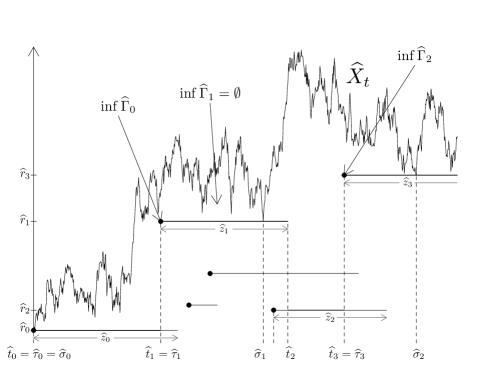
Figure 4: One realization of the graphical construction of thinned Model I. In contrast to Model I, there is the set of times $\Sigma_{\infty}=\{\widehat{\sigma}_{0},\widehat{\sigma}_{1},\widehat{\sigma}_{2},...\}$ which serve as renewal points for the process. For example, note that the reflection boundary between $\widehat{t}_{2}$ and $\widehat{t}_{3}$ is lower than in Figure 1.

Remark 5 (Renewal times for the thinned Model I)

Again, $\widehat{t}_{0},\widehat{t}_{1},\widehat{t}_{2},\dots$ are times when the reflection boundary changes for the thinned Model I. Moreover, the set $\Sigma_{n}$ consists of all first times after changing the reflection boundary, when $X_{t}=R_{t}$, up to $\widehat{t}_{n}$. Clearly, the additional restriction $\sup\Sigma_{n+1}\leq\tau$ in the definition of $(\widehat{t}_{n+1},\widehat{\tau}_{n+1},\widehat{z}_{n+1})$ in (3.4) leads to taking less Poisson points and hence $\widehat{R}_{t}\leq R_{t}$ and $\widehat{X}_{t}\leq X_{t}$ for all $t\geq 0$, almost surely. Moreover, the times $\Sigma_{\infty}:=\bigcup_{n=0}^{\infty}\Sigma_{n}$ are renewal times for the process $(\widehat{X}_{t}-\widehat{R}_{t})_{t\geq 0}$: We have $\widehat{X}_{t}-\widehat{R}_{t}=0$ for $t\in\Sigma_{\infty}$ and after time $t$, any reflection boundary $r$ with $(\tau,r,z)\in\mathcal{N}^{\gamma,\delta}$ must fulfill $\tau\geq t$ in the thinned Model I. In other words, the possible Poisson points for the reflection boundary before and after time $t$ are distinct, so the distributions of $(\widehat{X}_{s}-\widehat{R}_{s})_{0\leq s<t}$ and $(\widehat{X}_{s}-\widehat{R}_{s})_{s\geq t}$ are independent.

Using the renewal structure of the thinned Model I allows us to define a cumulative process.

Lemma 1 (Renewal structure)

Let $(\widehat{X}_{t},\widehat{R}_{t})_{t\geq 0}$ be a broken Brownian ratchet, thinned Model I, and $\Sigma_{\infty}=\{\widehat{\sigma}_{0},\widehat{\sigma}_{1},\dots\}$. Then, $(\widehat{\sigma}_{n}-\widehat{\sigma}_{n-1},\widehat{X}_{\widehat{\sigma}_{n}}-\widehat{X}_{\widehat{\sigma}_{n-1}})_{n=1,2,\dots}$ is a sequence of bivariate iid random variables.

Proof

By the construction of the thinned Model I, possible reflection boundaries $r$ with $(\tau,r,z)\in\mathcal{N}^{\gamma,\delta}$ are only used in one interval $[\widehat{\sigma}_{0},\widehat{\sigma}_{1}),[\widehat{\sigma}_{1},\widehat{\sigma}_{2}),[\widehat{\sigma}_{2},\widehat{\sigma}_{3}),\dots$ Hence, the Poisson points used for constructing $(\widehat{\sigma}_{n}-\widehat{\sigma}_{n-1},\widehat{X}_{\widehat{\sigma}_{n}}-\widehat{X}_{\widehat{\sigma}_{n-1}})_{n\geq 1}$ arise independently, which shows the result. ∎

Remark 6 (The thinned Model I as a cumulative process)

Let $(\widehat{X}_{t},\widehat{R}_{t})_{t\geq 0}$ be the $\gamma/\delta$-Brownian ratchet, thinned Model I. For $\Sigma_{\infty}=\{\widehat{\sigma}_{0},\widehat{\sigma}_{1},\dots\}$, set

$$M_{t}:=\min\{n:\widehat{\sigma}_{n}>t\},\quad S_{n}:=\sum_{i=1}^{n}{(\widehat{X}_{\widehat{\sigma}_{i}}-\widehat{X}_{\widehat{\sigma}_{i-1}})},$$ (3.6)

so that we have $\widehat{X}_{t}=S_{M_{t}}+A_{t}$, where

$$A_{t}:=\widehat{X}_{\widehat{\sigma}_{0}}+\widehat{X}_{t}-\widehat{X}_{\widehat{\sigma}_{M_{t}}}.$$ (3.7)

According to the definition of cumulative processes in Roginsky (1994), the thinned broken Brownian ratchet $\mathcal{X}$ is a type A cumulative process with remainder $A_{t}$. Note that finite first moments of $\widehat{\sigma}_{1}-\widehat{\sigma}_{0}$ and $X_{\widehat{\sigma}_{1}}-X_{\widehat{\sigma}_{0}}$ are sufficient for the strong law of large numbers for $S_{M_{t}}$. We will see that a law of large numbers holds also for $(\widehat{X}_{t})_{t\geq 0}$, as we will show in Proposition 2 that $A_{t}/t$ converges to 0 almost surely as $t\rightarrow\infty$.

Lemma 2 (Finite first moments of $\sigma$)

Consider a thinned Model I, started with $\widehat{X}_{0}=x\geq 0$ and

$$\widehat{\sigma}_{0}:=\inf\{t\geq 0:\widehat{X}_{t}=\widehat{R}_{t}\},$$ (3.8)

that is, $\widehat{\sigma}_{0}$ is the first time when then broken Brownian ratchet hits the moving reflection boundary. Then, using $\mathbb{E}_{x}[\cdot]:=\mathbb{E}[\cdot|X_{0}=x]$,

$$\sup_{x}{\mathbb{E}_{x}[\widehat{\sigma}_{0}]}<\infty.$$

Proof

Set $H_{t}:=\widehat{X}_{t}-\widehat{R}_{t}$ and note that $\mathcal{H}=(H_{t})_{t\geq 0}$ locally behaves like Brownian motion, and has jump discontinuities which, by time $t$, either increase or decrease $H_{t-}$. First, $H_{t-}$ jumps to $h<H_{t-}$ at rate $\gamma dh$ by occurrence of a new Poisson point in the graphical construction at rate $\gamma$. Second, it jumps to some $h>H_{t-}$ at rate $\delta$ since $t=\tau+z$ for the active Poisson point $(\tau,r,z)$ by time $t-$. Note that $\widehat{\sigma}_{0}:=\inf\{t\geq 0:H_{t}=0\}$. We couple the process $(H_{t})_{t\geq 0}$ to a process $(I_{t})_{t\geq 0}$ with $H_{t}\leq I_{t}$ for all $0\leq t\leq\widehat{\sigma}_{0}$, define $\sigma_{I}:=\inf\{t\geq 0:I_{t}=0\}$ and show that $\sup_{x}\mathbb{E}_{x}[\sigma_{I}]<\infty$.

The process $\mathcal{I}=(I_{t})_{t\geq 0}$ has the following dynamics: it behaves locally like the same Brownian motion as $\mathcal{H}$, but starts in $I_{0}=\infty$. It jumps to 1 at time $t$ in the following cases: (i) if $\mathcal{H}$ jumps from $H_{t-}>1$ to $H_{t}\leq 1$ (ii) if $\mathcal{H}$ jumps from $H_{t-}<1$ to $H_{t}\leq H_{t-}$ (iii) at an independent rate $\gamma(1-H_{t})^{+}$. In total this gives a jump rate of $\gamma$ to jump to 1 and $H_{t}\leq I_{t}$ at such a jump time. In addition, $\mathcal{I}$ jumps to $\infty$ if $\mathcal{H}$ jumps from $H_{t-}$ to $H_{t}>H_{t-}$, which occurs at rate $\delta$.

Consider an exponentially distributed random variable $T$ with rate $\gamma+\delta$ and a Brownian motion, starting in 1 at time $0$. Let $\sigma_{B}$ be its hitting time of 0 and set $p:=\mathbb{P}(\sigma_{B}\leq T)>0$. Note that $\sigma_{I}$ is given as follows: A Poisson point at rate $\gamma$ has to occur at time $s$ with the property that the Brownian motion, starting in 1 at time $s$ hits 0 before any of the other events, bringing $\mathcal{I}$ back to 1 or infinity, occurs. We obtain

$$\mathbb{E}_{x}[\sigma_{I}]=\frac{1}{p\gamma}+\mathbb{E}[\sigma_{B}|\sigma_{B}<T]=\frac{1}{p\gamma}+\frac{\mathbb{E}[\sigma_{B},\sigma_{B}<T]}{p}\leq\frac{1}{p}\Big{(}\frac{1}{\gamma}+\frac{1}{\gamma+\delta}\Big{)}<\infty,$$

independently of $x$. The result follows since $\widehat{\sigma}_{0}\leq\sigma_{I}$, almost surely. ∎

Lemma 3 (Increments of $(\widehat{X}_{t})_{t\geq 0}$)

For the $\gamma/\delta$-broken Brownian ratchet, thinned Model I, started in $x\geq 0$, we have

1. $\mathbb{E}_{x}[\widehat{X}^{2}_{\widehat{\sigma}_{0}}]<\infty$,

2. $0<\mathbb{E}_{x}[\widehat{X}_{\widehat{\sigma}_{1}}-\widehat{X}_{\widehat{\sigma}_{0}}]<\infty$,

3. $0<\mathbb{E}_{x}[\widehat{\sigma}_{1}-\widehat{\sigma}_{0}]<\infty$.

Proof

For (i), note that $|\widehat{X}_{\widehat{\sigma}_{0}}|\stackrel{{\scriptstyle d}}{{=}}|B_{\rho_{0}}|$. Using the second Wald identity and Lemma 2 we obtain

$$\mathbb{E}_{x}[\widehat{X}^{2}_{\widehat{\sigma}_{0}}]=\mathbb{E}_{x}[B^{2}_{\widehat{\sigma}_{0}}]=\mathbb{E}_{x}[\widehat{\sigma}_{0}]<\infty,$$

which shows (i). For (ii) and (iii), we can assume that $x=0$ and $\widehat{\sigma}_{0}=0$ without loss of generality. Consider the time $\widehat{t}$ of the first jump of $(\widehat{R}_{t})_{t\geq 0}$. Of course, we have $\widehat{X}_{\widehat{t}}>0$ almost surely and therefore $0<\mathbb{E}[\widehat{X}_{\widehat{t}}]<\infty$. Moreover, we have that $(\widehat{X}_{\widehat{\sigma}_{1}\wedge t}-\widehat{X}_{\widehat{t}})_{t\geq\widehat{t}}$ is a uniformly integrable martingale. Indeed, again using the second Wald identity and Lemma 2,

$$\sup_{t\geq\widehat{t}}\mathbb{E}_{x}[(\widehat{X}_{\widehat{\sigma}_{1}\wedge t}-\widehat{X}_{\widehat{t}})^{2}]=\sup_{t\geq\widehat{t}}\mathbb{E}_{x}[\widehat{\sigma}_{1}\wedge t-\widehat{t}\;]=\mathbb{E}_{x}[\widehat{\sigma}_{1}-\widehat{t}\;]<\infty.$$

By the Optional Stopping Theorem we obtain that

$$\mathbb{E}_{0}[\widehat{X}_{\widehat{\sigma}_{1}}]=\mathbb{E}_{0}[\widehat{X}_{\widehat{t}}]+\mathbb{E}_{0}[\widehat{X}_{\widehat{\sigma}_{1}}-\widehat{X}_{\widehat{t}}]=\mathbb{E}_{0}[\widehat{X}_{\widehat{t}}]$$

and (ii) follows since $0<\mathbb{E}[\widehat{X}_{\widehat{t}}]<\infty$. For (iii), rewrite $\widehat{\sigma}_{1}=(\widehat{\sigma}_{1}-\widehat{t})+\widehat{t}$. We know that $\widehat{t}$ is bounded from above by the killing time $\tau$ of a Brownian motion, if it is killed at rate $\gamma|B_{t}|$ at time $t$. In Depperschmidt and Pfaffelhuber (2010, Lemma 5.4) it was shown that $\mathbb{E}_{0}[\tau]<\infty$. Hence, by Lemma 2,

$$\mathbb{E}_{0}[\widehat{\sigma}_{1}] =\mathbb{E}_{0}[\widehat{\sigma}_{1}-\widehat{t}]+\mathbb{E}_{0}[\,\widehat{t}\;]$$

$$=\mathbb{E}_{0}\left[\mathbb{E}_{\widehat{X}_{\widehat{t}}-\widehat{R}_{\widehat{t}}}[\widehat{\sigma}_{0}]\right]+\mathbb{E}_{0}[\,\widehat{t}\;]\leq\sup_{x\geq 0}\mathbb{E}_{x}[\widehat{\sigma}_{0}]+\mathbb{E}_{0}[\tau]<\infty,$$

which finishes the proof. ∎

Proposition 2

Recall from Remark 6 the $\gamma/\delta$-broken Brownian ratchet as a cumulative process with remainder $(A_{t})_{t\geq 0}$ from (3.6). Then,

$$\lim_{t\rightarrow\infty}\frac{A_{t}}{t}=0\quad\text{ almost surely.}$$

Proof

We proceed as in Lemma 8 in Smith (1955). Define for $n=1,2,\dots$

$$Y_{n}=\sup_{t\in[\widehat{\sigma}_{n-1},\widehat{\sigma}_{n}]}|\widehat{X}_{t}-\widehat{X}_{\widehat{\sigma}_{n}}|$$

and note that $Y_{1},Y_{2},\dots$ are independent and identically distributed. We write, using Lemma 3(i) and the law of large numbers for $(M_{t})_{t\geq 0}$

$$\lim_{t\to\infty}\frac{|A_{t}|}{t} \leq\lim_{t\to\infty}\frac{|\widehat{X}_{\widehat{\sigma}_{0}}|}{t}+\lim_{t\to\infty}\frac{|\widehat{X}_{t}-\widehat{X}_{\widehat{\sigma}_{M_{t}}}|}{t}\leq\lim_{t\to\infty}\frac{M_{t}}{t}\cdot\lim_{t\to\infty}\frac{Y_{M_{t}}}{M_{t}}$$ (3.9)

$$=\frac{1}{\mathbb{E}[\widehat{\sigma}_{1}-\widehat{\sigma}_{0}]}\cdot\lim_{n\to\infty}\frac{Y_{n}}{n}.$$

Since $Y_{1}\leq\widehat{X}_{\widehat{\sigma}_{1}}+\sup_{t\geq 0}\widehat{X}_{t\wedge\widehat{\sigma}_{1}}$, by Doob’s inequality,

$$\mathbb{E}[Y_{1}^{2}]\leq 2\mathbb{E}[\widehat{X}_{\widehat{\sigma}_{1}}^{2}]+2\mathbb{E}[\sup_{t\geq 0}\widehat{X}_{t\wedge\widehat{\sigma}_{1}}^{2}]\leq 2\mathbb{E}[\widehat{X}_{\widehat{\sigma}_{1}}^{2}]+8\mathbb{E}[\widehat{X}_{\widehat{\sigma}_{1}}^{2}]<\infty,$$

it follows that $Y_{n}/n\to 0$ almost surely, as $n\to\infty$ by Lemma 7 in Smith (1955). Now, the result is implied by (3.9). ∎

3.3 Proof of Theorem 2.1

The proof consists of three steps. We derive the lower and upper bound for the speed of the broken ratchet. Then, we prove the scaling property.

Step 1: Lower bound for the speed: The thinned Model I of the $\gamma/\delta$-broken Brownian ratchet uses less possible reflection boundaries, leading to a smaller speed. Hence, if we can show that it still has positive speed we obtain that Model I has positive speed as well, as claimed in Theorem 2.1.

In order to prove that thinned Model I has a positive speed, we use the law of large numbers for the cumulative process as introduced in Remark 6. By the law of large numbers for $(S_{n})_{n=1,2,\dots}$ and $(M_{t})_{t\geq 0}$, Lemma 3 and Proposition 2, we have

$$\frac{\widehat{X}_{t}}{t} =\frac{S_{M_{t}}}{M_{t}}\frac{M_{t}}{t}+\frac{A_{t}}{t}\xrightarrow{t\to\infty}\frac{\mathbb{E}[\widehat{X}_{\widehat{\sigma}_{1}}-\widehat{X}_{\widehat{\sigma}_{0}}]}{\mathbb{E}[\widehat{\sigma}_{1}-\widehat{\sigma}_{0}]}=:c\text{ almost surely.}$$

Step 2: Upper bound for the speed: The speed of the $\gamma/\delta$-broken Brownian ratchet is decreasing in $\delta$. In particular, taking $\delta=0$ gives an upper bound for the speed. Moreover this bound is independent of $\delta$. We find from Depperschmidt and Pfaffelhuber (2010) that

$$\frac{X_{t}^{\gamma,\delta}}{t}\leq\frac{X_{t}^{\gamma,0}}{t}\xrightarrow{t\to\infty}C\text{ almost surely.}$$

for some $0<C<\infty$.

Step 3: Scaling property: As a consequence of Proposition 1 we have

$$\liminf_{t\rightarrow\infty}\frac{\mathbb{E}[X_{t}^{\gamma;\delta}]}{t} =\liminf_{t\rightarrow\infty}\gamma^{-\frac{1}{3}}\frac{\mathbb{E}[X_{\gamma^{2/3}t}^{1;\delta/\gamma^{2/3}}]}{t}=\liminf_{t\rightarrow\infty}\gamma^{\frac{1}{3}}\frac{\mathbb{E}[X_{\gamma^{2/3}t}^{1;\delta/\gamma^{2/3}}]}{\gamma^{2/3}t}$$

$$=\liminf_{t\rightarrow\infty}\gamma^{\frac{1}{3}}\frac{\mathbb{E}[X_{t}^{1;\delta/\gamma^{2/3}}]}{t}$$

where $\liminf$ can as well be replaced by $\limsup$.

4 Proofs: Model II

We start in Section 4.1, Proposition 3, with showing the same scaling property as given in Proposition 1 for Model I. The rest of the section is concerned with concrete calculations. Model II is linked to killed Brownian motion in Section 4.2. We interpret Model II as a (random) additive functional of a Markov chain, where the related Markov chain is defined in Definition 5 and is shown to have a unique equilibrium in Propositions 4 and 5 in Section 4.3. For this equilibrium, it is possible to compute increments analytically, which is carried out in the proof of Theorem 2.2 in Section 4.4.

4.1 Scaling property

The following result is the analogous result of Proposition 1 for Model II.

Proposition 3 (Scaling property, Model II)

Let $(\widetilde{X}_{t}^{\gamma;\delta},\widetilde{R}_{t}^{\gamma;\delta})_{t\geq 0}$ be the $\gamma/\delta$-broken Brownian ratchet, Model II, with $\gamma>0,\delta\geq 0$ and initial value $(0,0)$. Then, the following holds:

$$(\widetilde{X}_{t}^{\gamma;\delta},\widetilde{R}_{t}^{\gamma;\delta})_{t\geq 0}\overset{d}{=}\gamma^{-\frac{1}{3}}\left(\widetilde{X}_{\gamma^{2/3}t}^{1;\delta/\gamma^{2/3}},\widetilde{R}_{\gamma^{2/3}t}^{1;\delta/\gamma^{2/3}}\right)_{t\geq 0}.$$ (4.1)

Proof

We use supercripts $\gamma,\delta$ in order to emphasize dependency on the parameters and start with the $(\widetilde{X}_{t}^{\gamma,\delta},\widetilde{R}_{t}^{\gamma,\delta})_{t\geq 0}$-ratchet. Recall the notation from the proof of Proposition 1 as well as $\widetilde{g}(N^{\gamma})\stackrel{{\scriptstyle d}}{{=}}N^{1}$. Note that the rate-$\delta$ random variables $Z^{\delta}_{1},Z^{\delta}_{2},\dots$ in Definition 2 only affect the $t$-direction, while the random variables $E_{1}^{\gamma;\delta},E_{2}^{\gamma;\delta},E_{3}^{\gamma;\delta},\dots$ at rate $\gamma/\delta$ affect the $x$-direction. Since, $\widetilde{g}_{\gamma}(Z^{\delta}_{n},E_{n}^{\gamma;\delta})\stackrel{{\scriptstyle d}}{{=}}(Z_{n}^{\delta/\gamma^{2/3}},E_{n}^{1;\delta/\gamma^{2/3}})$, and since the same rescaling as in (3.2) holds in Model II, we have shown that

$$\gamma^{1/3}(\widetilde{X}_{t}^{\gamma;\delta},\widetilde{R}_{t}^{\gamma;\delta})_{t\geq 0}\stackrel{{\scriptstyle d}}{{=}}(\widetilde{X}_{\gamma^{2/3}t}^{1;\delta/\gamma^{2/3}},\widetilde{R}_{\gamma^{2/3}t}^{1;\delta/\gamma^{2/3}})_{t\geq 0}$$

and the assertion follows. ∎

4.2 Connections to killed Brownian motion

The Brownian motion which drives the broken Brownian ratchet, Model II, is reflected at the same boundary until $R_{t}$ changes. We interpret the time when this happens as a killing time of the Brownian motion. Due to the scaling property of the Brownian ratchet it would be possible to carry out the computations in the notationally convenient case $\gamma=\frac{1}{2}$ and deduce the general result from this particular one. However, we feel that an approach explicitly allowing for all values of $\gamma$ is more transparent.

Definition 4 (Killed reflected Brownian motion)

Let $(B_{t})_{t\geq 0}$ denote Brownian motion started in $x\geq 0$ and consider the stopping time $\eta$ defined by

$$\eta:=\inf\Big{\{}t>0:\int_{0}^{t}(\gamma|B_{s}|+\delta)\,ds\geq\xi\Big{\}},$$ (4.2)

where $\xi$ is an independent exponentially distributed random variable of rate $1$.

Define $\widetilde{\mathcal{B}}:=(\widetilde{B}_{t})_{t\geq 0}$ by $\widetilde{B}_{t}:=|B_{t}|$ for $0\leq t<\eta$ and $\widetilde{B}_{t}=\Delta$ for $t\geq\eta$, where $\Delta\not\in\mathbb{R}$ is the cemetery state. Then $\widetilde{\mathcal{B}}^{x}=\widetilde{\mathcal{B}}$ is reflected Brownian motion killed at rate $\gamma\widetilde{B}_{t}+\delta$ at time $t$. Denote the probability measure of the Brownian motion started in $x$ by $\mathbb{P}_{x}$ and write $\mathbb{E}_{x}$ for the respective expectation.

The second order operator $\mathcal{A}$ associated to the killed Brownian motion defined above acts on $C^{2}$ functions $f:[0,\infty)\to\mathbb{R}$ satisfying $f^{\prime}(0+)=0$ according to

$$\mathcal{A}f(x)=\frac{1}{2}f^{\prime\prime}(x)-(\gamma x+\delta)f(x).$$ (4.3)

The diffusion process $\widetilde{\mathcal{B}}$ is transient since it can be killed in each interval with positive probability. Let $p(\cdot;\cdot,\cdot)$ denote the corresponding transition density with respect to the speed measure which is given by $m(dx)=2dx$ (see Borodin and Salminen (2002, p. 17)). In the same way as in the proof of Lemma 5.4. in Depperschmidt and Pfaffelhuber (2010), the Green function of $\widetilde{\mathcal{B}}^{x}$ is given by

$$G(x,y):=\int_{0}^{\infty}p(t;x,y)\,dt,$$

which is finite for each $x,y\geq 0$. It can be written in terms of solutions of the differential equation $\mathcal{A}u=0$ which reads

$$u^{\prime\prime}(x)-(2\gamma x+2\delta)u(x)=0.$$ (4.4)

The following lemma is the basis for all calculations to follow.

Lemma 4 (Green function of killed Brownian motion)

The Green function of the killed Brownian motion from Definition 4 is given by

$$G(x,y):=\frac{1}{w}\begin{cases}\psi(x)\phi(y)&\text{for }0\leq x\leq y,\\ \psi(y)\phi(x)&\text{for }0\leq y\leq x,\end{cases}$$ (4.5)

where

$$w =\frac{(2\gamma)^{1/3}}{\pi},$$ (4.6)

and

$$\phi(x) =Ai\Big{(}(2\gamma)^{1/3}x+\tfrac{2^{1/3}\delta}{\gamma^{2/3}}\Big{)},$$ (4.7)

$$\psi(x) =Bi\Big{(}(2\gamma)^{1/3}x+\tfrac{2^{1/3}\delta}{\gamma^{2/3}}\Big{)}-CAi\Big{(}(2\gamma)^{1/3}x+\tfrac{2^{1/3}\delta}{\gamma^{2/3}}\Big{)},$$ (4.8)

with

$$C =C(\gamma,\delta)=\frac{Bi^{\prime}(\tfrac{2^{1/3}\delta}{\gamma^{2/3}})}{Ai^{\prime}(\tfrac{2^{1/3}\delta}{\gamma^{2/3}})}$$ (4.9)

are two solutions of (4.4).

Proof

In order to compute the Green function of the killed Brownian motion we need two particular solutions, say $f$ and $g$, of the equation (4.4) on $[0,\infty)$ such that (see e.g. Borodin and Salminen, 2002, p. 18–19)

1. $f$ is positive, strictly decreasing and $f(x)\to 0$ as $x\to\infty$,

2. $g$ is positive, strictly increasing,

3. $g^{\prime}(0)=0$ (this is the condition for reflecting boundary).

The functions $x\mapsto Ai\Big{(}(2\gamma)^{1/3}x+\tfrac{2^{1/3}\delta}{\gamma^{2/3}}\Big{)}$ and $x\mapsto Bi\Big{(}(2\gamma)^{1/3}x+\tfrac{2^{1/3}\delta}{\gamma^{2/3}}\Big{)}$ are two linearly independent solutions of (4.4). It is easy to check that the requirements (i)–(iii) are satisfied by functions $f=\phi$ and $g=\psi$ defined in (4.7) respectively (4.8).

The Wronskian of $\psi$ and $\phi$ is given by

$$w =\psi^{\prime}(0)\phi(0)-\psi(0)\phi^{\prime}(0)=-\psi(0)\phi^{\prime}(0)$$ (4.10)

$$=(2\gamma)^{1/3}\big{(}Bi^{\prime}(\tfrac{2^{1/3}\delta}{\gamma^{2/3}})Ai(\tfrac{2^{1/3}\delta}{\gamma^{2/3}})-Bi(\tfrac{2^{1/3}\delta}{\gamma^{2/3}})Ai^{\prime}(\tfrac{2^{1/3}\delta}{\gamma^{2/3}})\big{)}=\frac{(2\gamma)^{1/3}}{\pi},$$

hence all results follow from (see e.g. Borodin and Salminen, 2002, p. 18-19). ∎

The density of the killing position with respect to Lebesgue measure is $k(y)=2\gamma y+2\delta$ and moreover, the killing position of the Brownian motion started in $x$ has density

$$f(y):=G(x,y)k(y)$$ (4.11)

with respect to Lebesgue measure (see Borodin and Salminen, 2002, p. 17 resp. p. 14).

The next lemma will be used in the proof of Proposition 4.

Lemma 5 (Bounds on increments of killed Brownian motion)

For any $x\geq 0$

$$\frac{\phi(0)\psi(0)}{w}\leq\mathbb{E}_{x}[\widetilde{B}_{\eta-}]\leq x+\frac{\phi(0)\psi(0)}{w}.$$ (4.12)

Proof

Using the fact that $\psi$ and $\phi$ solve (4.4) and then integration by parts we obtain

$$\mathbb{E}_{x}[\widetilde{B}_{\eta-}] =\int_{0}^{\infty}yG(x,y)k(y)\,dy$$

$$=\frac{\psi(x)}{w}\int_{x}^{\infty}y\phi(y)(2\gamma y+2\delta)\,dy+\frac{\phi(x)}{w}\int_{0}^{x}y\psi(y)(2\gamma y+2\delta)\,dy$$

$$=\frac{\psi(x)}{w}\int_{x}^{\infty}y\phi^{\prime\prime}(y)\,dy+\frac{\phi(x)}{w}\int_{0}^{x}y\psi^{\prime\prime}(y)\,dy$$

$$=\frac{x}{w}(-\psi(x)\phi^{\prime}(y)+\phi(x)\psi^{\prime}(x))+\frac{\phi(x)\psi(0)}{w}=x+\frac{\phi(x)\psi(0)}{w}.$$

Now using the fact that $\phi$ is strictly decreasing we obtain the upper bound in (4.12). Furthermore, due to $\psi^{\prime}(0)=0$ by the choice of $C$ we have $\psi(0)=-w/\phi^{\prime}(0)=-w/Ai^{\prime}(\tfrac{2^{1/3}\delta}{\gamma^{2/3}})$. As the function

$$x\mapsto x+\frac{\phi(x)\psi(0)}{w}=x-\frac{Ai\Big{(}(2\gamma)^{1/3}x+\tfrac{2^{1/3}\delta}{\gamma^{2/3}}\Big{)}}{Ai^{\prime}(\tfrac{2^{1/3}\delta}{\gamma^{2/3}})}$$

is strictly increasing on $[0,\infty)$ its minimum is attained in $x=0$. This gives the lower bound in (4.12). ∎

4.3 The invariant distribution for increments at jump times

One advantage of Model II as compared to Model I is that we can define a Markov chain which models time- and space-increments at jump times of the reflection boundary. We show that the Markov chain has an equilibrium (Proposition 4) which is unique (Proposition 5).

Definition 5 (Markov chain at jump times)

Consider the $\gamma/\delta$-broken Brownian ratchet $(\widetilde{X}_{t},\widetilde{R}_{t})_{t\geq 0}$ from Definition 2 with $\widetilde{X}_{0}=x$ and $\widetilde{R}_{0}=0$. Define $(Y_{n},W_{n},\eta_{n},)_{n\geq 1}$ by

$$Y_{n}:=\widetilde{X}_{\tilde{t}_{n}}-\tilde{r}_{n},\quad W_{n}:=\tilde{r}_{n}-\tilde{r}_{n-1}\quad\text{and}\quad\eta_{n}:=\tilde{t}_{n}-\tilde{t}_{n-1}.$$ (4.13)

Note that for any $k$, $(Y_{n},W_{n},\eta_{n})_{n=k+1,k+2,\ldots}$ depends on $(Y_{n},W_{n},\eta_{n})_{n=1,2,\ldots,k}$ only through $Y_{k}$. That is, $(Y_{n},W_{n},\eta_{n},)_{n\geq 1}$ is a Markov chain. For any $n\geq 1$ we denote the law of $(Y_{n},W_{n},\eta_{n})_{n\geq 1}$ by $(P^{n}_{x})$.

Remark 7 (Distribution of $Y_{n}$ and $W_{n}$)

Let $(E_{n})_{n=0,1,\dots}$ be iid exponentially distributed with parameter $\gamma/\delta$ and let $(U_{n})_{n=0,1,\dots}$ be iid uniformly distributed on $[0,1]$. Then, recalling Definition 2,

$$Y_{n+1} \stackrel{{\scriptstyle d}}{{=}}\begin{cases}(\widetilde{X}_{\tilde{t}_{n+1}}-\tilde{r}_{n})(1-U_{n}),&\text{ if }\tilde{r}_{n+1}>\tilde{r}_{n},\\ (\widetilde{X}_{\tilde{t}_{n+1}}-\tilde{r}_{n}+E_{n}),&\text{ if }\tilde{r}_{n+1}\leq\tilde{r}_{n},\end{cases}$$

and

$$W_{n+1} \stackrel{{\scriptstyle d}}{{=}}\begin{cases}(\widetilde{X}_{\tilde{t}_{n+1}}-\tilde{r}_{n})U_{n},&\text{ if }\tilde{r}_{n+1}>\tilde{r}_{n},\\ -E_{n},&\text{ if }\tilde{r}_{n+1}\leq\tilde{r}_{n}\end{cases}$$

where $\stackrel{{\scriptstyle d}}{{=}}$ means equality in distribution. In particular, on the event $\{\tilde{r}_{n+1}>\tilde{r}_{n}\}$ the random variables $W_{n+1}$ and $Y_{n+1}$ have the same distribution.

In the following two propositions we obtain existence and uniqueness of the invariant distribution of the Markov chain $(Y_{n},W_{n},\eta_{n})_{n\geq 1}$.

Proposition 4 (Existence of invariant distribution)

For any $x\geq 0$ the sequence of Cesàro averages $\left(n^{-1}\sum_{k=1}^{n}{P^{k}_{x}}\right)_{n\geq 1}$ converges along a subsequence weakly to an invariant distribution $P_{x}$ of the Markov chain $(Y_{n},W_{n},\eta_{n})_{n\geq 1}$.

Proof

In the case $\delta=0$ the assertion is shown in Proposition 5.6 in Depperschmidt and Pfaffelhuber (2010). Thus, we assume $\delta>0$ in the rest of the proof. We only need to show that the first moments of $Y_{n}$, $W_{n}$ and $\eta_{n}$ are bounded uniformly in $n$. This implies that the sequence $(P_{x}^{n})_{n\geq 1}$ is tight. Then the sequence of Cesàro averages $\left(n^{-1}\sum_{k=1}^{n}{P^{k}_{x}}\right)_{n\geq 1}$ is also tight. That is, any subsequence contains another subsequence along which the Cesàro averages converge weakly. These weak limits are invariant for the Markov chain $(Y_{n},W_{n},\eta_{n})_{n\geq 1}$. A proof of this fact in the continuous time case, that can be easily adapted to the discrete time case, can be found in Liggett (1985, p. 11).

The moments of each $\eta_{n}$ are bounded from above, since by construction, see (2.5), each $\eta_{n}$ is bounded by an exponential random variable with parameter $\delta$. Furthermore by construction we have (see Remark 7)

$$Y_{n+1} =(\widetilde{X}_{\tilde{t}_{n+1}}-\tilde{r}_{n})\big{(}{\mathds{1}}_{\{\tilde{r}_{n+1}>\tilde{r}_{n}\}}(1-U_{n})+{\mathds{1}}_{\{\tilde{r}_{n+1}\leq\tilde{r}_{n}\}}\big{)}+{\mathds{1}}_{\{\tilde{r}_{n+1}\leq\tilde{r}_{n}\}}E_{n}$$

$$\leq(\widetilde{X}_{\tilde{t}_{n+1}}-\tilde{r}_{n})(1-{\mathds{1}}_{\{\tilde{r}_{n+1}>\tilde{r}_{n}\}}U_{n})+E_{n}.$$

We set $\mathcal{G}_{n}=\sigma((\widetilde{X}_{t},\widetilde{R}_{t})_{0\leq t\leq\tilde{t}_{n}})$ and $c:=\phi(0)\psi(0)/w$. By the strong Markov property we obtain

$$\mathbb{E}[(\widetilde{X}_{\tilde{t}_{n+1}}-\tilde{r}_{n})|\mathcal{G}_{n}]=\mathbb{E}_{Y_{n}}[\widetilde{X}_{\tilde{t}_{1}}-\tilde{r}_{0}]=\mathbb{E}_{Y_{n}}[\widetilde{B}_{\eta-}],$$

where $\widetilde{B}_{t}$ is killed reflecting Brownian motion from Definition 4 and $\eta$ is its killing time. Furthermore

$$\mathbb{E}[(\widetilde{X}_{\tilde{t}_{n+1}}-\tilde{r}_{n}){\mathds{1}}_{\{\tilde{r}_{n+1}>\tilde{r}_{n}\}}|\mathcal{G}_{n}]=\mathbb{E}_{Y_{n}}[(\widetilde{X}_{\tilde{t}_{1}}-\tilde{r}_{0}){\mathds{1}}_{\{\tilde{r}_{1}>\tilde{r}_{0}\}}]=\mathbb{E}_{Y_{n}}\left[\frac{\widetilde{B}_{\eta-}^{2}}{\widetilde{B}_{\eta-}+\delta/\gamma}\right].$$

The function $x\mapsto x^{2}/(x+\delta/\gamma)$ is convex. Thus, by Jensen’s inequality

$$\mathbb{E}[(\widetilde{X}_{\tilde{t}_{n+1}}-\tilde{r}_{n}){\mathds{1}}_{\{\tilde{r}_{n+1}>\tilde{r}_{n}\}}|\mathcal{G}_{n}]\geq\mathbb{E}_{Y_{n}}[\widetilde{B}_{\eta-}]\frac{\mathbb{E}_{Y_{n}}[\widetilde{B}_{\eta-}]}{\mathbb{E}_{Y_{n}}[\widetilde{B}_{\eta-}]+\delta/\gamma}.$$

Now using that the function $x\mapsto x/(x+\delta/\gamma)$ is increasing and (4.12) we obtain

$$\mathbb{E}[(\widetilde{X}_{\tilde{t}_{n+1}}-\tilde{r}_{n}){\mathds{1}}_{\{\tilde{r}_{n+1}>\tilde{r}_{n}\}}|\mathcal{G}_{n}]\geq\mathbb{E}_{Y_{n}}[\widetilde{B}_{\eta-}]\frac{c}{c+\delta/\gamma}.$$

Altogether, setting

$$q:=1-\frac{1}{2}\frac{c}{c+\delta/\gamma}\in(0,1)$$

we obtain

$$\mathbb{E}_{x}[Y_{n+1}] \leq\mathbb{E}_{x}[(\widetilde{X}_{\tilde{t}_{n+1}}-\tilde{r}_{n})(1-{\mathds{1}}_{\{\tilde{r}_{n+1}>\tilde{r}_{n}\}}U_{n})+E_{n}]$$

$$=\mathbb{E}_{x}\left[\mathbb{E}[(\widetilde{X}_{\tilde{t}_{n+1}}-\tilde{r}_{n})(1-{\mathds{1}}_{\{\tilde{r}_{n+1}>\tilde{r}_{n}\}}U_{n})|\mathcal{G}_{n}]\right]+\delta/\gamma$$

$$\leq q\mathbb{E}_{x}\left[\mathbb{E}_{Y_{n}}[\widetilde{B}_{\eta-}]\right]+\delta/\gamma$$

$$\leq q(\mathbb{E}_{x}[Y_{n}]+c)+\delta/\gamma,$$

where we used (4.12) for the last inequality. Uniform boundedness of the first moments of $Y_{n}$ follows since the recursion $x_{n+1}=qx_{n}+d$ has a unique fixed point for $|q|<1$ and any $d$. For $W_{n+1}$ we have

$$W_{n+1} ={\mathds{1}}_{\{\tilde{r}_{n+1}>\tilde{r}_{n}\}}U_{n}(\widetilde{X}_{\tilde{t}_{n+1}}-\tilde{r}_{n})-{\mathds{1}}_{\{\tilde{r}_{n+1}\leq\tilde{r}_{n}\}}E_{n}.$$

Now using that on $\{\tilde{r}_{n+1}>\tilde{r}_{n}\}$, $W_{n+1}=|W_{n+1}|$ and $Y_{n+1}$ have the same distribution we obtain

$$\mathbb{E}_{x}[|W_{n+1}|]=\mathbb{E}_{x}[{\mathds{1}}_{\{\tilde{r}_{n+1}>\tilde{r}_{n}\}}Y_{n+1}+{\mathds{1}}_{\{\tilde{r}_{n+1}\leq\tilde{r}_{n}\}}E_{n}]\leq\mathbb{E}_{x}[Y_{n+1}]+\delta/\gamma.$$

Uniform boundedness of first moments of $W_{n}$ follows from uniform boundedness of first moments of $Y_{n}$. ∎

Proposition 5 (Uniqueness of invariant distribution)

Consider the Markov chain $(Y_{n},W_{n},\eta_{n})_{n=1,2,\dots}$ from Definition 5 on the basis of a broken Brownian ratchet, Model II started in $x\geq 0$. If an invariant distribution of the Markov chain exists, then it is unique.

Proof

In the proof we use a second graphical construction for the $\gamma/\delta$-broken Brownian ratchet, Model II, $(\widetilde{X}_{t},\widetilde{R}_{t})_{t\geq 0}$, which is based on a single Brownian motion $(B_{t})_{t\geq 0}$ with $B_{0}=0$; see also Figure 5(A).

We define the sequence of active points $(S_{n})_{n=0,1,\dots}$, the sequence of reflection boundaries $(R_{n})_{n=0,1,\dots}$ and a sequence of jump times $(\kappa_{n})_{n=0,1,\dots}$ as follows: Let $(\xi_{n})_{n=0,1,\dots}$ be iid exponentially distributed with parameter $1$, $(E_{n})_{n=0,1,\dots}$ iid exponentially distributed with parameter $\gamma/\delta$, and let $(U_{n})_{n=0,1,\dots}$ be iid uniformly distributed on $(0,1)$. We define $\kappa_{0}=0$, $S_{0}=x$, $R_{0}=0$ and for $n\geq 0$

$$\kappa_{n+1} =\inf\Big{\{}t>\kappa_{n}:\int_{\kappa_{n}}^{t}(\gamma|B_{s}-S_{n}|+\delta)\,ds\geq\xi_{n}\Big{\}}$$

is the time of the next event after $\kappa_{n}$ with rate $\gamma|B_{s}-S_{n}|+\delta$ at time $s$. At time $\kappa_{n+1}$, there are two possibilities:

• If $\{S_{n}\geq B_{\kappa_{n+1}}\}$, set

  $$(S_{n+1},R_{n+1}) =\begin{cases}(S_{n}-U_{n}(S_{n}-B_{\kappa_{n+1}}),R_{n}+U_{n}(S_{n}-B_{\kappa_{n+1}}))\\ \phantom{(S_{n}+E_{n},R_{n}-E_{n})}\text{ with probability }\frac{\gamma|B_{\kappa_{n+1}}-S_{n}|}{\gamma|B_{\kappa_{n+1}}-S_{n}|+\delta},\\ (S_{n}+E_{n},R_{n}-E_{n})\text{ with probability }\frac{\delta}{\gamma|B_{\kappa_{n+1}}-S_{n}|+\delta}.\end{cases}$$

• If $\{S_{n}<B_{\kappa_{n+1}}\}$, set

  $$(S_{n+1},R_{n+1}) =\begin{cases}(S_{n}+U_{n}(B_{\kappa_{n+1}}-S_{n}),R_{n}+U_{n}(B_{\kappa_{n+1}}-S_{n}))\\ \phantom{(S_{n}-E_{n},R_{n}-E_{n})}\text{ with probability }\frac{\gamma|B_{\kappa_{n+1}}-S_{n}|}{\gamma|B_{\kappa_{n+1}}-S_{n}|+\delta},\\ (S_{n}-E_{n},R_{n}-E_{n})\text{ with probability }\frac{\delta}{\gamma|B_{\kappa_{n+1}}-S_{n}|+\delta}.\end{cases}$$

Thus, the active point jumps uniformly between the currently active point and the Brownian motion at rate $\gamma$ times their distance or it jumps an exponential distance away from the Brownian motion. In particular,

$$R_{n+1} =\begin{cases}R_{n}+U_{n}|B_{\kappa_{n+1}}-S_{n}|&\text{ with probability }\frac{\gamma|B_{\kappa_{n+1}}-S_{n}|}{\gamma|B_{\kappa_{n+1}}-S_{n}|+\delta},\\ R_{n}-E_{n}&\text{ with probability }\frac{\delta}{\gamma|B_{\kappa_{n+1}}-S_{n}|+\delta},\end{cases}$$

i.e. the reflection boundaries either jump up at rate $\gamma$ times the distance of the Brownian motion to the active point or down at rate $\delta$.

Now set

$$\widetilde{R}_{t} =R_{n},\quad\widetilde{S}_{t}=S_{n},\quad\text{for $t\in[\kappa_{n},\kappa_{n+1})$}$$

and

$$\widetilde{X}_{t} =\widetilde{R}_{t}+|B_{t}-\widetilde{S}_{t}|\quad\text{for $t\geq 0$.}$$

Then, $(\widetilde{X}_{t})_{t\geq 0}$ is reflected at $(\widetilde{R}_{t})_{t\geq 0}$ and is continuous, since for all $n\geq 1$,

$$\widetilde{X}_{\kappa_{n+1}-} =R_{n}+|B_{\kappa_{n+1}-}-S_{n}|,$$

$$\widetilde{X}_{\kappa_{n+1}} =\begin{cases}R_{n}+U_{n}|B_{\kappa_{n+1}-}-S_{n}|+|B_{\kappa_{n+1}}-S_{n}-U_{n}(B_{\kappa_{n+1}}-S_{n})|\\ \qquad\qquad\qquad\qquad\qquad\qquad\text{ with probability }\frac{\gamma|B_{\kappa_{n+1}}-S_{n}|}{\gamma|B_{\kappa_{n+1}}-S_{n}|+\delta},\\ R_{n}-E_{n}+|B_{\kappa_{n+1}}-S_{n}|+E_{n}\\ \qquad\qquad\qquad\qquad\qquad\qquad\text{ with probability }\frac{\delta}{\gamma|B_{\kappa_{n+1}}-S_{n}|+\delta}\end{cases}$$

$$=R_{n}+|B_{\kappa_{n+1}}-S_{n}|.$$

In other words, the process $(\widetilde{X}_{t},\widetilde{R}_{t})_{t\geq 0}$ is a $\gamma/\delta$-broken Brownian ratchet, Model II starting in $(|x|,0)$.

We now prove Proposition 5 using a coupling argument, illustrated in Figure 5(B). Recall that a coupling of two $\gamma/\delta$-broken Brownian ratchets, Model II, is a process $(\widetilde{X}_{t}^{(1)},\widetilde{R}_{t}^{(1)},\widetilde{X}_{t}^{(2)},\widetilde{R}_{t}^{(2)})$ such that $(\widetilde{X}_{t}^{(i)},\widetilde{R}_{t}^{(i)})$ is a $\gamma/\delta$-broken Brownian ratchet, $i=1,2$. It is straightforward, using the same Brownian motion, to construct such a coupling along the lines of the above construction, where $(\widetilde{X}_{t}^{(1)},\widetilde{R}_{t}^{(1)})$ starts in $(x^{(1)},0)$ and $(\widetilde{X}_{t}^{(2)},\widetilde{R}_{t}^{(2)})$ in $(x^{(2)},0)$, respectively, for $x^{(1)},x^{(2)}\geq 0$. Then, we must show that both broken ratchets use the same active points after an almost surely finite time. This suffices, since from this time on the time- and space-increments at jump times are the same for both processes, and hence, both must converge to the same limit law (see e.g. Lindvall, 1992, Thm. 21.12).

In order to show that both broken ratchets use the same active points after finite time, note the following: if the active points of both ratchets are both above or both below the Brownian motion they have a chance to jump to the same point (see Figure 5(B)). Assume for definiteness that at time $t$ we have $\widetilde{S}_{t}^{(2)}<\widetilde{S}_{t}^{(1)}<B_{t}$ (as at time $t$ in Figure 5(B)). Then at rate $\gamma(\widetilde{S}_{t}^{(2)}-\widetilde{S}_{t}^{(1)})$ only the lower active point jumps towards the $B_{t}$ and if it does, it jumps uniformly between $\widetilde{S}_{t}^{(1)}$ and $\widetilde{S}_{t}^{(2)}$. Furthermore at rate $\gamma(B_{t}-S_{t}^{(2)})$ both jump to the same uniform position between $S_{t}^{(2)}$ and $B_{t}$. From then on the active points evolve together and we refer to this time as the coupling time ($T_{c}$ in Figure 5(B)). After the coupling time both ratchets have the same jump times and the same increments. Since the Brownian motion will spend infinite amount of time below or above both active points the coupling time is almost surely finite. ∎

(A)                                             (B)

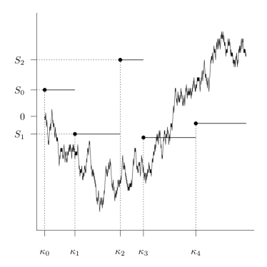
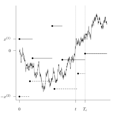
Figure 5: (A) Alternative graphical construction of Model II from the proof of Proposition 5. (B) Graphical construction of two coupled $\gamma/\delta$-broken Brownian ratchet, Model II, using the same Brownian motion, similar to (A). After time $\text{T}_{\text{coupl}}$ the active points and the jump times of active points are the same for both processes.

4.4 Proof of Theorem 2.2

The proof of Theorem 2.2 comes in three steps. First, we will connect the speed of the broken Brownian ratchet, Model II, to the Markov chain $(Y_{n},W_{n},\eta_{n})_{n\geq 1}$ from Definition 5, and show that the speed equals the ratio of expected space- and time-increments between jump times. In Step 2, we use the unique equilibrium of this Markov chain to obtain a fixed point equation for $Y$, which allows to study its density. In Step 3, we use insights into the density of $Y$ in order to study expected increments between jump times.

Step 1: Connection to the Markov chain $(Y_{n},W_{n},\eta_{n})$: In the last section we have established the unique equilibrium distribution $\pi$ for the Markov chain $(Y_{n},W_{n},\eta_{n})_{n\geq 1}$. Let $(Y,W,\eta)$ be distributed according to $\pi$ and recall that $Y$ is the distance of the Brownian ratchet to its reflection boundary at jump times, $W$ is the amount by which the reflection boundary jumps and $\eta$ is the time between jumps. Note that $\eta$ equals the killing time of the Brownian motion as introduced in Definition 4, if the Brownian motion is started in an independent copy of $Y$.

The proof works along similar lines as in the proof of Theorem 1 in Depperschmidt and Pfaffelhuber (2010). Formally, Model II is a cumulative process similar to the thinned Model I; see Remark 6. Renewal points are times when the Brownian ratchet hits the reflection boundary, given a jump of the reflection boundary occurred between renewal points. The law of large numbers for cumulative processes establishes that $X_{t}/t$ converges as $t\to\infty$ to the ratio of expected space- and time increments between renewal times, almost surely; compare with (4.14) below. Then, proceeding exactly as in the proof of Theorem 1 in Depperschmidt and Pfaffelhuber (2010, p. 923), it can be seen from the ratio limit theorem (see e.g. Revuz, 1984, Thm. 6.6 on p. 231) that

$$\lim_{t\to\infty}\frac{X_{t}}{t}=\frac{\mathbb{E}[W]}{\mathbb{E}[\eta]}.$$ (4.14)

Step 2: A distributional identity and some consequences: The triple $(Y,W,\eta)$ is distributed according to the equilibrium $\pi$. Starting the Brownian ratchet in position $Y$, the reflection boundary at the next jump time either jumps up or down. Let $U$ be uniformly distributed on $[0,1]$ and denote the length of the possible downward jump by $Z$, distributed as $\mathrm{Exp}\left(\delta/\gamma\right)$. By construction

$$Y\stackrel{{\scriptstyle d}}{{=}}{\mathds{1}}_{\{\text{jump up at $\eta$}\}}\widetilde{B}^{Y}_{\eta-}U+{\mathds{1}}_{\{\text{jump down at $\eta$}\}}\left(\widetilde{B}^{Y}_{\eta-}+Z\right).$$ (4.15)

Conditioned on the event that the reflection boundary jumps at time $\eta$ the probability of an upward jump is

$$\frac{\gamma\widetilde{B}^{Y}_{\eta-}}{\gamma\widetilde{B}^{Y}_{\eta-}+\delta}=\frac{\widetilde{B}^{Y}_{\eta-}}{\widetilde{B}^{Y}_{\eta-}+\delta/\gamma}$$

and for a downward jump

$$\frac{\delta}{\gamma\widetilde{B}^{Y}_{\eta-}+\delta}=\frac{\delta/\gamma}{\widetilde{B}^{Y}_{\eta-}+\delta/\gamma}.$$

Let us write $f_{X}$ for the density of a random variable $X$. Equations (4.15) and (4.11) imply

$$f_{Y}(z) =\int_{0}^{\infty}\!\!\!\!f_{Y}(x)\int_{0}^{\infty}\!\!\!\!f_{\widetilde{B}^{x}_{\eta-}}(u)\left(\frac{u}{u+\delta/\gamma}f_{U}\left(\frac{z}{u}\right)\frac{1}{u}+\frac{\delta/\gamma}{u+\delta/\gamma}f_{Z}(z-u)\right)\,du\,dx$$

$$=\int_{0}^{\infty}f_{Y}(x)\int_{z}^{\infty}f_{\widetilde{B}^{x}_{\eta-}}(u)\frac{1}{u+\delta/\gamma}\,du\,dx$$

$$\qquad\qquad\qquad\qquad+\int_{0}^{\infty}f_{Y}(x)\int_{0}^{z}f_{\widetilde{B}^{x}_{\eta}}(u)\frac{\delta/\gamma}{u+\delta/\gamma}\frac{\gamma}{\delta}e^{-(z-u)\gamma/\delta}\,du\,dx$$

$$=2\gamma\underbrace{\int_{0}^{\infty}f_{Y}(x)\int_{z}^{\infty}G(x,u)\,du\,dx}_{=:A(z)}$$

$$\qquad\qquad\qquad\qquad+2\gamma\underbrace{\int_{0}^{\infty}f_{Y}(x)\int_{0}^{z}G(x,u)e^{-(z-u)\gamma/\delta}du\;dx}_{=:B(z)}.$$

In particular we have

$$f_{Y}(0)=2\gamma A(0)=2\gamma\int_{0}^{\infty}f_{Y}(x)\int_{0}^{\infty}G(x,u)\,du\,dx.$$ (4.16)

We aim at showing that the pair $(A,B)$ satisfies the differential equation (2.7). For that we need to differentiate $A$ and $B$. The derivatives of $A$ and $B$ are readily computed as

$$A^{\prime}(z) =-\frac{1}{w}\left[\psi(z)\int_{z}^{\infty}{f_{Y}(x)\phi(x)dx}+\phi(z)\int_{0}^{z}{f_{Y}(x)\psi(x)dx}\right]$$

$$\text{and}\quad B^{\prime}(z) =-A^{\prime}(z)-\frac{\gamma}{\delta}B(z).$$

Thus,

$$f^{\prime}_{Y}(z) =2\gamma(A^{\prime}(z)+B^{\prime}(z))=-\frac{2\gamma^{2}}{\delta}B(z).$$ (4.17)

For $A$ we have

$$A(z) =\int_{0}^{\infty}f_{Y}(x)\int_{z}^{\infty}G(x,u)\,du\,dx,$$ (4.18)

$$A^{\prime}(z) =-\frac{1}{w}\left[\psi(z)\int_{z}^{\infty}{f_{Y}(x)\phi(x)dx}+\phi(z)\int_{0}^{z}{f_{Y}(x)\psi(x)dx}\right],$$

$$A^{\prime\prime}(z) =-\frac{1}{w}\left[\psi^{\prime}(z)\int_{z}^{\infty}{f_{Y}(x)\phi(x)dx}+\phi^{\prime}(z)\int_{0}^{z}{f_{Y}(x)\psi(x)dx}\right],$$ (4.19)

$$\begin{split}A^{\prime\prime\prime}(z)&=-\frac{1}{w}\Bigl{[}\psi^{\prime\prime}(z)\int_{z}^{\infty}{f_{Y}(x)\phi(x)dx}+\phi^{\prime\prime}(z)\int_{0}^{z}{f_{Y}(x)\psi(x)dx}\\ &\qquad-f_{Y}(z)(\psi^{\prime}(z)\phi(z)-\psi(z)\phi^{\prime}(z))\Bigr{]}\\ &=f_{Y}(z)+(2\gamma z+2\delta)A^{\prime}(z),\end{split}$$

where we have used that $\phi$ and $\psi$ are solutions of (4.4), the equation for $A^{\prime}$ and that the Wronskian does not depend on $z$. Writing now $f_{Y}=2\gamma(A+B)$ and using (4.17) we obtain

$$A^{\prime\prime\prime}(z) =2\gamma(A(z)+B(z))+(2\gamma z+2\delta)A^{\prime}(z)$$

$$=-2\delta(A^{\prime}(z)+B^{\prime}(z))+2\gamma A(z)+(2\gamma z+2\delta)A^{\prime}(z)$$

$$=-2\delta B^{\prime}(z)+\left(2\gamma zA(z)\right)^{\prime}.$$

Integrating both sides we have

$$A^{\prime\prime}(z) =-2\delta B(z)+2\gamma zA(z).$$ (4.20)

The integration constant vanishes because $B(0)=0$ and $A^{\prime\prime}(0)=0$, as can be seen from (4.19) (recall that $\psi^{\prime}(0)=0$). Thus, $(A,B)$ is a solution of (2.7).

Step 3: Computation of $\mathbb{E}[W]$ and $\mathbb{E}[\eta]$: In the case that the reflection boundary jumps up $W$ and $Y$ have the same distribution. If the reflection boundary jumps down $W$ is distributed as $-Z$ where $Z$ is exponentially distributed with parameter $\gamma/\delta$. Thus, the density of the invariant distribution of $W$ is given by

$$f_{W}(z) =\int_{0}^{\infty}f_{Y}(x)\int_{0}^{\infty}f_{\widetilde{B}^{x}_{\eta-}}(u)\Big{(}\frac{u}{u+\delta/\gamma}{\mathds{1}}_{\{z\geq 0\}}f_{U}\left(\frac{z}{u}\right)\frac{1}{u}$$

$$\qquad\qquad\qquad\qquad\qquad\qquad\qquad+\frac{\delta/\gamma}{u+\delta/\gamma}f_{Z}(-z){\mathds{1}}_{\{z<0\}}\Big{)}\,du\,dx$$

$$=2\gamma A(z){\mathds{1}}_{\{z\geq 0\}}+\int_{0}^{\infty}f_{Y}(x)\int_{0}^{\infty}f_{\widetilde{B}^{x}_{\eta-}}(u)\frac{\delta/\gamma}{u+\delta/\gamma}\frac{\gamma}{\delta}e^{z\gamma/\delta}{\mathds{1}}_{\{z<0\}}\,du\,dx$$

$$=2\gamma A(z){\mathds{1}}_{\{z\geq 0\}}+e^{z\gamma/\delta}{\mathds{1}}_{\{z<0\}}\int_{0}^{\infty}f_{Y}(x)\int_{0}^{\infty}G(x,u)\,du\,dx$$

$$=2\gamma A(z){\mathds{1}}_{\{z\geq 0\}}+2\gamma e^{z\gamma/\delta}{\mathds{1}}_{\{z<0\}}A(0).$$

In order to compute $\mathbb{E}[W]$ we have to integrate the last equations. We use (4.20) and (4.17) and obtain

$$\mathbb{E}[W] =\int_{0}^{\infty}2\gamma zA(z)-2\gamma ze^{-z\gamma/\delta}A(0)dz$$ (4.21)

$$=\int_{0}^{\infty}A^{\prime\prime}(z)+2\delta B(z)dz-\frac{2\delta^{2}}{\gamma}A(0)$$

$$=-A^{\prime}(0)+\frac{\delta^{2}}{\gamma^{2}}f_{Y}(0)-\frac{\delta^{2}}{\gamma^{2}}f_{Y}(0)=-A^{\prime}(0).$$

Moreover, by (4.16) we have

$$\mathbb{E}[\eta]=2\int_{0}^{\infty}f_{Y}(x)\int_{0}^{\infty}G(x,y)\,dy\,dx=2A(0).$$ (4.22)

Here the factor $2$ shows up because we have to integrate the Green function with respect to the speed measure, which is $m(dy)=2\,dy$ in the case of Brownian motion.

Now, Theorem 2.2 follows from (4.14), (4.21) and (4.22), since multiplying $A$ by a constant factor does not change the ratio $-A^{\prime}(0)/(2A(0))$.

References

- Abdolvahab et al (2008) Abdolvahab RH, Roshani F, Nourmohammad A, Sahimi M, Tabar MR (2008) Analytical and numerical studies of sequence dependence of passage times for translocation of heterobiopolymers through nanopores. J Chem Phys 129:235,102
- Abdolvahab et al (2011) Abdolvahab RH, Roshani F, Nourmohammad A, Sahimi M, Tabar MR (2011) Sequence dependence of the binding energy in chaperone-driven polymer translocation through a nanopore. Phys Rev Letter E 83:011,902
- Abramowitz and Stegun (1972) Abramowitz M, Stegun IA (1972) Handbook of Mathematical Functions: with Formulas, Graphs, and Mathematical Tables, 10th edn. Dover Publications, New York
- Ambjornsson et al (1992) Ambjornsson T, Lomholt M, Metzler R (1992) Directed motion emerging from two coupled random processes: translocation of a chain through a membrane nanopore driven by binding proteins. J of Physics-condensed matter 17 47, Sp. Iss. SI:3945–3964
- Borodin and Salminen (2002) Borodin A, Salminen P (2002) Handbook of Brownian Motion - Facts and Formulae, 2nd edn. Birkhäuser Verlag
- Budhiraja and Fricks (2006) Budhiraja A, Fricks J (2006) Molecular Motors, Brownian Ratchets, and Reflected Diffusions. Discrete Contin Dyn Syst Series B 6:711–734
- Depperschmidt and Pfaffelhuber (2010) Depperschmidt A, Pfaffelhuber P (2010) Asymptotics of a brownian ratchet for protein translocation. Stochastic Processes and their Applications 120:901–925
- D’Orsogna et al (2007) D’Orsogna MR, Chou T, Antal T (2007) Exact steady-state velocity of ratchets driven by random sequential adsorption. J Phys A Math Gen 40:5575–5584
- Elston (2002) Elston T (2002) The Brownian ratchet and power stroke models for posttranslational protein translocation into the endoplasmatic reticulum. Biophys J 82:1239–1253
- Glick (1995) Glick BS (1995) Can Hsp70 proteins act as force-generating motors? Cell 80:11–14
- Griesemer et al (2007) Griesemer M, Young C, Raden D, Doyle F, Robinson A, Petzold L (2007) Computational Modeling of Chaperone Interactions in the Endoplasmic Reticulum of Saccharomyces Cerevisai
- Li and Chiu (2010) Li HM, Chiu CC (2010) Protein transport into chloroplasts. Annu Rev Plant Biol 61:157–180
- Liebermeister et al (2001) Liebermeister W, Rapoport T, Heinrich R (2001) Ratcheting in post-translational protein translocation: A mathematical model. J Mol Biol 305:643–656
- Liggett (1985) Liggett TM (1985) Interacting Particle Systems. Springer-Verlag
- Lindvall (1992) Lindvall T (1992) Lectures on the Coupling Method, 1st edn. Wiley
- Matlack et al (1999) Matlack KE, Misselwitz B, Plath K, Rapoport TA (1999) BiP acts as a molecular ratchet during posttranslational transport of prepro-alpha factor across the ER membrane. Cell 97:553–564
- Neupert and Brunner (2002) Neupert W, Brunner M (2002) The protein import motor of mitochondria. Nat Rev Mol Cell Biol 3:555–565
- Neupert and Herrmann (2007) Neupert W, Herrmann JM (2007) Translocation of proteins into mitochondria. Annu Rev Biochem 76:723–749
- Okamoto et al (2002) Okamoto K, Brinker A, Paschen SA, Moarefi I, Hayer-Hartl M, Neupert W, Brunner M (2002) The protein import motor of mitochondria: a targeted molecular ratchet driving unfolding and translocation. EMBO J 21:3659–3671
- Peskin et al (1993) Peskin C, Odell G, Oster G (1993) Cellular motions and thermal fluctuations: The brownian ratchet. Biophys J 65:316–324
- Pfanner and Truscott (2002) Pfanner N, Truscott KN (2002) Powering mitochondrial protein import. Nat Struct Biol 9:234–236
- Rapoport (2007) Rapoport TA (2007) Protein translocation across the eukaryotic endoplasmic reticulum and bacterial plasma membranes. Nature 450:663–669
- Revuz (1984) Revuz D (1984) Markov Chains, 2nd edn. American Elsevier, North-Holland
- Roginsky (1994) Roginsky AL (1994) A central limit theorem for cumulative processes. Adv Appl Prob 26:104–121
- Schneider et al (1994) Schneider HC, Berthold J, Bauer MF, Dietmeier K, Guiard B, Brunner M, Neupert W (1994) Mitochondrial Hsp70/MIM44 complex facilitates protein import. Nature 371:768–774
- Simon et al (1992) Simon S, Peskin C, Oster G (1992) What drives the translocation of proteins? Proc Natl Acad Sci USA 89:3770–3774
- Smith (1955) Smith W (1955) Regenerative stochastic processes. Proc Roy Soc London Ser. A. 232:6–31
- Strittmatter et al (2010) Strittmatter P, Soll J, Bolter B (2010) The chloroplast protein import machinery: a review. Methods Mol Biol 619:307–321
- Wickner and Schekman (2005) Wickner W, Schekman R (2005) Protein translocation across biological membranes. Science 310:1452–1456
- Zandi et al (2003) Zandi R, Reguera D, Rudnick J, Gelbart WM (2003) What drives the translocation of stiff chains? Proc Natl Acad Sci USA 100:8649–8653