Lattice permutations and Poisson-Dirichlet distribution of cycle lengths

Abstract

We study random spatial permutations on ${\mathbb{Z}}^{3}$ where each jump $x\mapsto\pi(x)$ is penalized by a factor $\,{\rm e}^{-T\|x-\pi(x)\|^{2}}\,$. The system is known to exhibit a phase transition for low enough $T$ where macroscopic cycles appear. We observe that the lengths of such cycles are distributed according to Poisson-Dirichlet. This can be explained heuristically using a stochastic coagulation-fragmentation process for long cycles, which is supported by numerical data.

1 Introduction

Random permutations are common in probability theory and combinatorics [4]. They also occur in statistical mechanics, albeit with an additional spatial structure. With $\Lambda$ denoting a finite box in ${\mathbb{Z}}^{3}$, we consider the set ${\mathcal{S}}_{\Lambda}$ of permutations of $\Lambda$, i.e., the set of bijections $\Lambda\to\Lambda$. The probability of a given permutation $\pi\in{\mathcal{S}}_{\Lambda}$ depends on the jump lengths in such a way that all sites are mapped in their neighborhoods. In this paper, we study the model with probability

$${\mathbb{P}}_{\Lambda}(\pi)=\frac{1}{Z_{\Lambda}}\exp\Big{(}-T\sum_{x\in\Lambda}\|x-\pi(x)\|^{2}\Big{)}\ .$$ (1)

Here $T>0$ is a positive parameter and $\|x-\pi(x)\|$ denotes the Euclidean distance between $x$ and $\pi(x)$. The normalization $Z_{\Lambda}$ is defined by

$$Z_{\Lambda}=\sum_{\pi\in{\mathcal{S}}_{\Lambda}}\exp\Big{(}-T\sum_{x\in\Lambda}\|x-\pi(x)\|^{2}\Big{)}\ .$$ (2)

This model has its origin in Feynman’s approach to the quantum Bose gas [13], where $T$ is proportional to the temperature. Bosons are described by Brownian trajectories with $\frac{1}{T}$ playing the rôle of time; this suggests the weights (1) for the permutation $\pi$. The presence of a lattice is not really justified, but it does not affect the qualitative behavior, at least in dimension 3 (we comment on dimension 2 at the end of the article).

Let us understand the qualitative behavior of the model when we vary the parameter $T$. The most probable permutation is the identity, which has weight $1$. Typical permutations should be close to the identity when $T$ is large, with small cycles here and there. The weight in (1) penalizes large jumps and we expect that $\|x-\pi(x)\|\lesssim\frac{1}{\sqrt{T}}$ . As $T$ decreases, sites are allowed to be mapped to more locations and the lengths of permutation cycles grow. One expects that a phase transition takes place (in dimension 3 or more) that is accompanied by the occurrence of infinite cycles. See Fig. 1 for a schematic spatial permutation with small $T$.

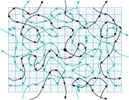
Figure 1: A typical spatial permutation with periodic boundary conditions for small $T$. The cycle that contains the origin is depicted in black and it may be long. Isolated sites belong to 1-cycles (i.e., they are mapped onto themselves).

The phase transition was observed numerically in [15, 17]; it takes place at $T_{\rm c}\approx 1.71$. The fraction of sites that belong to macroscopic cycles was seen to converge to a non-random function $\nu_{\infty}(T)$ as $|\Lambda|\to\infty$, which is continuous and monotone decreasing in $T$. There are many macroscopic cycles and their sizes fluctuate. It was also observed that the average length of the largest cycle scales like $0.624\nu_{\infty}(T)|\Lambda|$, which is identical to the expectation of the largest cycle in a random permutation with uniform distribution [23]. The latter observation was unexplained and puzzling at the time.

The situation is understood better now, and the explanation turns out to be surprisingly general. The joint distribution of the length of the long cycles is given by the Poisson-Dirichlet distribution. This distribution has been introduced by Kingman in [18] and has cropped up in combinatorics, population genetics, number theory, Bayesian statistics and probability theory, see [12, 19, 4, 20, 21] for details of applications and extensions.

Occurrence of the Poisson-Dirichlet distribution in models of statistical mechanics, i.e. in models with spatial structure, seems to have been noticed only recently. It has been rigorously established in the “annealed” model of spatial permutations where the locations of the sites are averaged upon [9]. The proof is inspired by [24] and it uses a representation in terms of occupation numbers of Fourier modes, and non-spatial permutations within the modes. Such a structure is not present here, however.

We recall the definition of the Poisson-Dirichlet distribution in Section 2.2 and provide numerical evidence in Section 2.3 that it is present in our model. In order to explain this, we show that the equilibrium state can be viewed as the stationary measure of an effective split-merge process. This strategy was recently applied successfully by Schramm to the random interchange model on the complete graph [22] (the result was first conjectured by Aldous, see [6]). The absence of spatial structure makes the situation much simpler, but it was nonetheless a tour de force to prove that long cycles occur, that they satisfy an effective split-merge process, and that their asymptotic distribution is Poisson-Dirichlet (see also [5] for subsequent simplifications and improvements). This strategy was also devised in [16] for the cycles and loops that arise in the Tóth and Aizenman-Nachtergaele representations of quantum Heisenberg models in three spatial dimensions [25, 2]. It allowed in particular to identify the parameter of the conjectured Poisson-Dirichlet distribution. Further situations that look similar include the random currents in the classical or quantum Ising models [1, 10, 14].

The key features are as follows: Long cycles are one-dimensional macroscopic objects and they are spread uniformly over the whole space. Introducing a suitable stochastic process with local changes, we observe that cycles are merged at a rate proportional to the number of “contacts” between them, and this number is proportional to the product of their lengths. Cycles are split at a rate proportional to the number of self-contacts, which is proportional to the square of the length. This is exactly analogous to a split-merge process on interval partitions [21, 3, 7]. As a consequence, the distribution of cycle lengths at equilibrium should be given by the invariant measure of the split-merge process, which is known to be the Poisson-Dirichlet distribution.

This explanation seems very attractive but it glosses over many technicalities. It assumes that a spatially uniform distribution of long cycles leads to a “mean-field” interaction and the correlations due to their spatial structure can be ignored. We provide mathematical background for these ideas in Section 3.1 and this allows us to state precise conjectures in Section 3.2. These conjectures are confronted with numerical results in Section 3.3. As it turns out, the above heuristics is fully confirmed.

2 Distribution of long cycles

2.1 Nature of long cycles

Let us first give precise definitions for “macroscopic”, “mesoscopic” and “finite” cycles in the infinite volume limit. Given $x\in\Lambda$ and a permutation $\pi\in{\mathcal{S}}_{\Lambda}$, let $L_{x}(\pi)$ denote the length of the cycle that contains $x$, i.e., the number of sites in the support of this cycle.

• Macroscopic cycles occupy a non-zero fraction of the volume. The fraction of sites in macroscopic cycles is given by

  $$\nu_{\rm macro}(T)=\lim_{\varepsilon\to 0^{+}}\liminf_{|\Lambda|\to\infty}\frac{1}{|\Lambda|}{\mathbb{E}}_{\Lambda}\Bigl{(}\#\{x\in\Lambda:L_{x}>\varepsilon|\Lambda|\}\Bigr{)}.$$ (3)

• Mesoscopic cycles are infinite cycles that are not macroscopic. The fraction of sites in mesoscopic cycles is given by

  $$\nu_{\rm meso}(T)=\lim_{K\to\infty}\liminf_{|\Lambda|\to\infty}\frac{1}{|\Lambda|}{\mathbb{E}}_{\Lambda}\Bigl{(}\#\{x\in\Lambda:K<L_{x}<\frac{|\Lambda|}{K}\}\Bigr{)}.$$ (4)

• Finally, the fraction of sites in finite cycles is given by

  $$\begin{split}\nu_{\rm finite}(T)&=\lim_{K\to\infty}\liminf_{|\Lambda|\to\infty}\frac{1}{|\Lambda|}{\mathbb{E}}_{\Lambda}\Bigl{(}\#\{x\in\Lambda:L_{x}<K\}\Bigr{)}\\ &=1-\nu_{\infty}(T).\end{split}$$ (5)

Here, $\nu_{\infty}(T)=\nu_{\rm meso}(T)+\nu_{\rm macro}(T)$ is the fraction of sites in infinite cycles.

One expects that only finite cycles are present when $T$ is large, that a phase with macroscopic cycles is present when $T$ is smaller than a positive number $T_{\rm c}$. This was proved in the annealed model in [8, 9]. We check this numerically in the lattice model. Let

$$\rho_{|\Lambda|}(a)={\mathbb{E}}_{\Lambda}\Bigl{(}\frac{\#\{x\in\Lambda:L_{x}\leq|\Lambda|^{a}\}}{|\Lambda|}\Bigr{)}.$$ (6)

denote the fraction of sites that belong to cycles of length less than or equal to $|\Lambda|^{a}$. Notice that $\rho_{|\Lambda|}(0)$ is the fraction of particles mapped onto themselves and that $\rho_{|\Lambda|}(1)=1$. Numerical results for $\rho_{|\Lambda|}(a)$ are depicted in Fig. 2 for various parameters $T$.

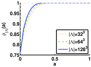
(a) $T=1.75>T_{c}$

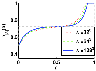
(b) $T=1.5<T_{c}$

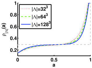
(c) $T=0.8<T_{c}$

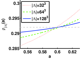
(d) $T=0.8$ (zoom)

Figure 2: Plots of the expected fraction of sites $\rho_{|\Lambda|}(a)$ in cycles of length smaller than or equal to $|\Lambda|^{a}$. The horizontal dashed line indicates $1-\nu_{\infty}(T)$, the fraction of particles in finite cycles in the infinite volume limit. The curves have an intersection point independent of $|\Lambda|$ at $a\approx 0.6$ which is therefore used as the cutoff to distinguish long and short cycles. $\nu_{\infty}(0.8)$ is estimated to be $0.292$. Averages were taken over $5\times 10^{4}$ realizations.

In a finite domain, we need to define the cutoff that separates finite and “infinite” cycles. We can choose $|\Lambda|^{a}$ with any power $0<a<1$, since in the infinite volume limit, $\rho_{\infty}(a)$ will not depend on our choice. The graphs of $\rho_{\Lambda}(a)$ depend on the size of the domain, but we see in Fig. 2 (d) that they cross the same point around $a\approx 0.6$ for $T<T_{c}$. This value of $a$ is approximately independent of $T$ and we choose it for the cutoff, since it significantly reduces finite size effects. For the numerical results, we define the fraction $\nu_{|\Lambda|}$ of sites that belong to infinite cycles by

$$\nu_{|\Lambda|}(T)=1-\rho_{|\Lambda|}(0.6).$$ (7)

In accordance with results for the annealed model [8, 9] we expect that $\nu_{\rm meso}(T)=0$ and that

$$\lim_{|\Lambda|\to\infty}\nu_{|\Lambda|}(T)=\nu_{\infty}(T)=\nu_{\rm macro}(T).$$ (8)

This is supported by the numerics in Fig. 2.

2.2 Griffiths-Engen-McCloskey and Poisson-Dirichlet distributions

For a given permutation $\pi\in{\mathcal{S}}_{\Lambda}$ we call the cycle at $x$ with length $L_{x}(\pi)$ macroscopic if $L_{x}(\pi)>|\Lambda|^{0.6}$, as discussed in the previous section. Let $L^{(1)}(\pi),L^{(2)}(\pi),\ldots,L^{(k)}(\pi)$ denote the cycle lengths in decreasing order, where $L^{(k)}$ is the smallest macroscopic cycle for the permutation $\pi$. If $\lambda^{(i)}=\frac{L^{(i)}}{|\Lambda|}$ is the fraction of the sites in the $i$th macroscopic cycle, we define

$$\nu(\pi):=\lambda^{(1)}+...+\lambda^{(k)}$$ (9)

to be the fraction of sites in macroscopic cycles, and have ${\mathbb{E}}_{\Lambda}(\nu)=\nu_{|\Lambda|}(T)$. The sequence $(\lambda^{(i)})$ forms a random partition of the (random) interval $[0,\nu(\pi)]$. We now introduce the relevant measures on such partitions, that will allow us to describe the joint distribution of cycle lengths.

The Poisson-Dirichlet distribution (PD) is a one-parameter family but we only need the distribution with parameter $1$, so we ignore the paramter altogether. It is best introduced with the help of the Griffiths-Engen-McClosckey distribution (GEM). The latter is also called the “stick-breaking” distribution. One can generate a random sequence of positive numbers $(\lambda_{1},\lambda_{2},\dots)$ such that $\sum_{i}\lambda_{i}=\nu$ as follows:

• choose $\lambda_{1}$ uniformly in $[0,\nu]$;

• choose $\lambda_{2}$ uniformly in $[0,\nu-\lambda_{1}]$;

• choose $\lambda_{3}$ uniformly in $[0,\nu-\lambda_{1}-\lambda_{2}]$;

• and so on…, always chopping a piece off the remaining portion of the “stick”.

This is equivalent to choosing a sequence of i.i.d. random variables $(\alpha_{1},\alpha_{2},\dots)$ where each $\alpha_{i}$ is taken uniformly in $[0,1]$, and then to form the sequence

$$(\alpha_{1},(1-\alpha_{1})\alpha_{2},(1-\alpha_{1})(1-\alpha_{2})\alpha_{3},\dots)\times\nu.$$

Our goal is to recognize that a given sequence has the distribution GEM. One can invert the above construction, and form an i.i.d. sequence out of a GEM sequence. Namely, if $(\lambda_{1},\lambda_{2},\dots)$ is GEM on the interval $[0,\nu]$, the following sequence is i.i.d. with respect to the uniform distribution on $[0,1]$:

$$(\alpha_{1},\alpha_{2},\alpha_{3},\dots)=\Bigl{(}\frac{\lambda_{1}}{\nu},\frac{\lambda_{2}}{\nu-\lambda_{1}},\frac{\lambda_{3}}{\nu-\lambda_{1}-\lambda_{2}},\dots\Bigr{)}.$$ (10)

PD is a distribution on ordered partitions, and a PD sequence can be obtained by rearranging a GEM sequence in decreasing order. On the other hand, given an ordered PD sequence, a GEM sequence can be obtained as a size-biased permutation of that sequence [21].

2.3 Numerical observations of cycle lengths

The GEM distribution is easier to handle than the PD distribution, and it contains more information. We thus introduce an order on cycles allowing us to establish an order for the cycle lengths. This can be done as follows. First, choose an order for the sites of $\Lambda$. Then order the cycles according to the smallest sites in their support; namely, given two cycles $\gamma=(x_{1},\ldots,x_{|\gamma|})$ and $\gamma^{\prime}=(x^{\prime}_{1},\ldots,x^{\prime}_{|\gamma^{\prime}|})$, we say that $\gamma<\gamma^{\prime}$ if and only if $\min_{1\leq i\leq|\gamma|}x_{i}<\min_{1\leq i\leq|\gamma^{\prime}|}x^{\prime}_{i}$. We then denote $L_{1},\,L_{2},\ldots$ the lengths of cycles larger than $|\Lambda|^{0.6}$ in this order, which is not to be confused with the notation $L_{x}$ for lengths of cycles rooted in $x\in\Lambda$.

Let $\nu\equiv\nu(\pi)$ for a given permutation. Our aim is to show that $(\frac{L_{1}}{\nu\left|\Lambda\right|},\frac{L_{2}}{\nu\left|\Lambda\right|}...)$ converges to GEM as $|\Lambda|\to\infty$, as illustrated in Fig. 3. This is equivalent to showing that

$$(\alpha_{1},\alpha_{2},\alpha_{3},\dots)=\Bigl{(}\frac{L_{1}}{\nu\left|\Lambda\right|},\frac{L_{2}}{\nu\left|\Lambda\right|-L_{1}},\frac{L_{3}}{\nu\left|\Lambda\right|-L_{1}-L_{2}},...\Bigr{)}$$ (11)

converges to a sequence of i.i.d. uniform random variables in $[0,1]$, see Eq. (10).

Figure 3: The lengths of macroscopic cycles, divided by the volume, give a random partition of $[0,\nu]$ which is expected to follow the GEM distribution.

The Cumulative Distribution Function for $\alpha_{i}$ is defined as

$$F_{\alpha_{i}}(s)=P(\alpha_{i}\leq s).$$ (12)

Numerical plots of $F_{\alpha_{i}}$ for the first three cycles can be found in Fig. 4. They clearly point to uniform random variables. Covariances can be found in Fig. 5, showing that they do indeed tend to $0$ in the infinite volume limit. The discontinuities at $s=1$ in Fig. 4 for $i=1,2,3$ are due to the fact that in finite volumes it may happen that only $0,1,2$ cycles larger than $|\Lambda|^{0.6}$, respectively, are present.

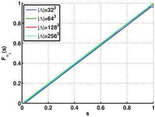
(a) $F_{\alpha_{1}}(s)$

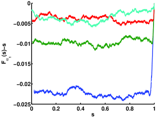
(b) $F_{\alpha_{1}}(s)-s$

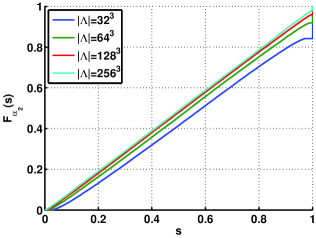
(c) $F_{\alpha_{2}}(s)$

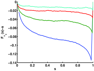
(d) $F_{\alpha_{2}}(s)-s$

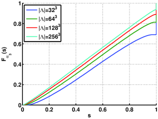
(e) $F_{\alpha_{3}}(s)$

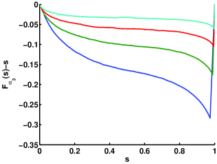
(f) $F_{\alpha_{3}}(s)-s$

Figure 4: Cumulative distribution functions $F_{\alpha_{i}}(s)$ (12) with $i=1,2,3$ for system sizes $|\Lambda|=32^{3},\ 64^{3},\ 128^{3},\ 256^{3}$ and $T=0.8$. As the volume tends to infinity, they converge to the CDF of a uniform random variable. Averages were taken over $10^{5}$ realizations.

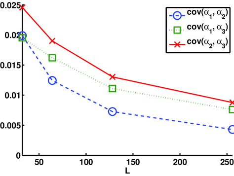
Figure 5: Covariances of $\alpha_{1},\alpha_{2},\alpha_{3}$ as given in (11) shown for different system sizes $|\Lambda|=32^{3},\ 64^{3},\ 128^{3},\ 256^{3}$ and $T=0.8$.

2.4 Markov chain Monte-Carlo

To sample spatial permutations we use a Markov chain Monte-Carlo process which is ergodic and has ${\mathbb{P}}_{\Lambda}$ as its unique stationary distribution. Let $B_{\Lambda}$ denote a suitable set of bonds, i.e., a set of unordered pairs $\{x,y\}$ of sites $x,y\in\Lambda$. Let $\tau_{xy}=\tau_{yx}$ denote the transposition of $x$ and $y$. We say that two permutations $\pi,\pi^{\prime}\in S_{\Lambda}$ are “in contact”, noted $\pi\sim\pi^{\prime}$, if there exists a bond $\{x,y\}\in B_{\Lambda}$ such that $\pi^{\prime}=\pi\circ\tau_{xy}$. Let $Q(\pi,\pi^{\prime})$, $\pi,\pi^{\prime}\in{\mathcal{S}}_{\Lambda}$, be the transition matrix of a continuous-time Markov chain $(\pi_{t}:t\geq 0)$ on ${\mathcal{S}}_{\Lambda}$.

Proposition 2.1

Suppose that $B_{\Lambda}$ is large enough so that the graph $(\Lambda,B_{\Lambda})$ is connected, and that $Q(\pi,\pi^{\prime})>0$ whenever $\pi\sim\pi^{\prime}$. The Markov chain with transition rates $Q$ is ergodic.

Proof. This is done in [17], but we recall the argument here. The space ${\mathcal{S}}_{\Lambda}$ of lattice permutations is finite and irreducibility of the chain implies ergodicity. It then suffices to show that for all $\pi,\pi^{\prime}\in{\mathcal{S}}_{\Lambda}$, $\pi^{\prime}\neq\pi$ there exists $n<\infty$ such that $Q^{n}(\pi,\pi^{\prime})>0$. Every permutation $\pi$ can be represented by a composition of transpositions. We still need to show that each of these transpositions can be written as a composition of transpositions along bonds of $B_{\Lambda}$.

Since the graph $(\Lambda,B_{\Lambda})$ is connected, there exists a connected path $(x_{0},x_{1},\dots,x_{m})$ such that $x_{0}=x$, $x_{m}=y$, and $\{x_{i-1},x_{i}\}\in B_{\Lambda}$ for all $1\leq i\leq m$. One can check that the following composition gives $\tau_{x,y}$:

$$\tau_{x,y}=\tau_{x_{0},x_{1}}\circ\dots\circ\tau_{x_{m-2},x_{m-1}}\circ\tau_{x_{m-1},x_{m}}\circ\tau_{x_{m-2},x_{m-1}}\circ\dots\circ\tau_{x_{0},x_{1}}.$$ (13)

This shows that every $\pi\in{\mathcal{S}}_{\Lambda}$ is connected to the identity permutation under the Markov chain dynamics. $\square$

The composition of $\pi$ with a transposition is explicitly given by

$$(\pi\circ\tau_{xy})(z)=\pi\big{(}\tau_{xy}(z)\big{)}=\left\{\begin{array}[]{cl}\pi(z)&\mbox{if }z\neq x,y,\\ \pi(y)&\mbox{if }z=x,\\ \pi(x)&\mbox{if }z=y.\end{array}\right.\$$ (17)

Let $H_{\Lambda}(\pi)$ denote the “energy” of $\pi\in{\mathcal{S}}_{\Lambda}$,

$$H_{\Lambda}(\pi)=T\sum_{x\in\Lambda}\|x-\pi(x)\|^{2}\ .$$ (18)

Here the Euclidean distance $\|\cdot\|$ is measured with periodic boundary conditions on a regular box $\Lambda\in{\mathbb{Z}}^{3}$. The distribution (1) then assumes the familiar form of the Gibbs state $e^{-H_{\Lambda}(\pi)}/Z_{\Lambda}$. For the transition rates we choose

$$Q(\pi,\pi^{\prime})=\begin{cases}\frac{1}{|B_{\Lambda}|}\min(1,\,{\rm e}^{-(H_{\Lambda}(\pi^{\prime})-H_{\Lambda}(\pi))}\,)&\text{if }\pi^{\prime}\sim\pi,\\ 0&\text{otherwise.}\end{cases}$$ (19)

Note that all rates are in $[0,1]$ and can therefore be used as acceptance probabilities for the standard Metropolis algorithm: pick a bond $\{x,y\}\in B_{\Lambda}$ uniformly at random and swap the images of $x$ and $y$ under $\pi$ with probability $1$ if this lowers the energy, and with probability $e^{-(H_{\Lambda}(\pi^{\prime})-H_{\Lambda}(\pi))}<1$ if the swap increases the energy.

It is clear that the measure ${\mathbb{P}}_{\Lambda}$ fulfills the detailed balance conditions, since

$$e^{-H_{\Lambda}(\pi)}Q(\pi,\pi^{\prime})=e^{-H_{\Lambda}(\pi^{\prime})}Q(\pi^{\prime},\pi)$$ (20)

for all $\pi,\pi^{\prime}\in{\mathcal{S}}_{\Lambda}$. This implies stationarity.

The particular algorithm we use is the “swap only” method described in [17]. The initial permutation is set to be the identity. The Metropolis steps are then as follows:

• Choose a bond $\{x,y\}$ of nearest-neighbors at random (we use periodic boundary conditions).

• The candidate permutation, $\pi^{\prime}=\pi\circ\tau_{xy}$, replaces $\pi$ with probability $\min(1,e^{-(H_{\Lambda}(\pi^{\prime})-H_{\Lambda}(\pi))})$.

The Metropolis step is then computationally fast since $H_{\Lambda}(\pi\circ\tau_{xy})-H_{\Lambda}(\pi)$ depends only on local terms:

$$H_{\Lambda}(\pi\circ\tau_{xy})-H_{\Lambda}(\pi)=T\Big{(}\|x{-}\pi(y)\|^{2}+\|y{-}\pi(x)\|^{2}-\|x{-}\pi(x)\|^{2}-\|y{-}\pi(y)\|^{2}\Big{)}\ .$$ (21)

We use a standard approach based on the ergodic theorem for sampling, where we let the system equilibrate for a number of Metropolis steps of order $10^{3}|\Lambda|$, and ensure that our measurements are spread over $5\times 10^{3}|\Lambda|$ steps. We have strong numerical evidence that the equilibration time of relevant observables is indeed of order $|\Lambda|$, as is shown in Fig 6.

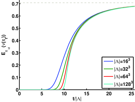
Figure 6: Expected value of the fraction of particles in macroscopic cycles for the permutation after $t$ Metropolis steps starting from the identity permutation, for $|\Lambda|=16^{3},\ 32^{3},\ 64^{3},\ 128^{3}$ and $T=0.8$. Rescaling time by $\frac{1}{|\Lambda|}$ shows the asymptotic behavior, showing that the equilibration time is of order $|\Lambda|$. The dashed line indicates the asymptote for the curves, $\nu_{\infty}(0.8)$. Averages were taken over $10^{4}$ realizations.

2.5 Periodic boundary conditions

We use periodic boundary conditions where $\Lambda\subset{\mathbb{Z}}^{3}$ is a 3-dimensional torus with equal side lengths $L$. This has the advantage of having less finite size effects than other choices such as closed boundary conditions. In the limit $|\Lambda|\to\infty$ we expect our results not to depend on that choice.

Precisely, for $y\in{\mathbb{Z}}^{d}$ we define $v_{i}(y)$ to be the $i$th component of $y$ modulo $L$, in such a way that $v_{i}(y)\in\{-\frac{L}{2}+1,\dots,\frac{L}{2}\}$ (we assume here that $L$ is even, but the modifications for odd $L$ are straighforward). The Euclidean distance on ${\mathbb{Z}}^{d}$ is then replaced by

$$\|y\|=\Bigl{(}\sum_{i=1}^{d}|v_{i}(y)|^{2}\Bigr{)}^{1/2}.$$ (22)

Permutations on the torus can be charaterized by their winding number, which is in reality a winding vector. The winding number of $\pi$ in the $i$th direction, $i=1,\dots,d$, is the integer

$$W_{i}(\pi)=\frac{1}{L}\sum_{x\in\Lambda}v_{i}(\pi(x)-x).$$ (23)

In a large box, one should not expect any jumps of order $L$ for positive $T>0$ because of the Gaussian weights (1). The dynamics restricted to such permutations conserves the winding number:

Proposition 2.2

Suppose that the permutation $\pi$ satisfies

$$\max_{x\in\Lambda}\|\pi(x)-x\|\leq\tfrac{L}{2}-2.$$

Then $W_{i}(\pi\circ\tau_{xy})=W_{i}(\pi)$ for all $i$ and all pairs $(x,y)$ of nearest-neighbors in $\Lambda$.

Proof. Using (17), we have

$$W_{i}(\pi\circ\tau_{xy})-W_{i}(\pi)=\tfrac{1}{L}v_{i}(\pi(y)-x)+\tfrac{1}{L}v_{i}(\pi(x)-y)-\tfrac{1}{L}v_{i}(\pi(x)-x)-\tfrac{1}{L}v_{i}(\pi(y)-y).$$ (24)

Because of the modulo operation, we have

$$\begin{split}&v_{i}(\pi(y)-x)=[\pi(y)-x]_{i}+k_{1}L,\quad&v_{i}(\pi(x)-x)=[\pi(x)-x]_{i}+k_{3}L,\\ &v_{i}(\pi(x)-y)=[\pi(x)-y]_{i}+k_{2}L,&v_{i}(\pi(y)-y)=[\pi(y)-y]_{i}+k_{4}L.\end{split}$$ (25)

Here, $[\cdot]_{i}$ denotes the $i$th coordinate of the vector in ${\mathbb{Z}}^{d}$, and we always have $k_{i}\in\{-1,0,1\}$. It follows from the assumptions that $k_{1}=k_{4}$ and $k_{2}=k_{3}$, so that (24) vanishes. $\square$

The consequence of this proposition is that we effectively lose ergodicity in very large systems, since the dynamics conserves the winding number on simulation time scales. On the other hand, when macroscopic cycles are present, we expect nonzero winding numbers to appear with positive probability in the equilibrium measure. The dynamics always start with the identity permutation which has zero winding number. By the proposition, the path to nonzero winding numbers must cross bottlenecks, i.e, permutations with large jumps which occur with probability less than $\frac{1}{Z}\,{\rm e}^{-T(\frac{L}{2}-1)^{2}}\,$. A big part of the phase space is not explored by the dynamics.

By introducing Monte-Carlo transitions that flip the orientations of cycles (which does not change their probability), it is easy to move between permutations with even winding numbers. On the other hand, it would be interesting to study the winding numbers of typical permutations at equilibrium, but this seems to be a very difficult task numerically since it requires dynamics that can move between odd an even winding numbers and still sample from the correct distribution.

Due to the metastability of the winding number, the actual mixing time of the Monte-Carlo dynamics is (at least) $\,{\rm e}^{cL^{2}}\,$ with $c>0$. However, since we are only interested in cycle lengths and not in their orientation, we do not expect this to be relevant for the observables discussed in the present paper. In fact, as is shown in Figure 6 and later in Figure 13, we observe convergence on time scales of order $|\Lambda|=L^{3}$. This is still much faster than processes such as card shuffles leading to uniform distributions on permutations (see e.g. [27]), which are typically of order $|\Lambda|^{3}$ with logarithmic corrections. This is due to the fact that for positive temperature $T$ the stationary distribution (1) is not uniform, and jumps in a typical permutation are local of order $1/\sqrt{T}$. Furthermore, the identity permutation we start with is actually the ground state (permutation with highest probability) of that measure.

3 Effective split-merge process

In the previous section we presented numerical evidence that the lengths of macroscopic cycles are distributed according to the Poisson-Dirichlet distribution. The goal of the present section is to explain it with a split-merge process, defined below in Section 3.1. More precisely, the Markov chain Monte-Carlo process of Section 2.4, when restricted to the cycle structure, becomes an effective split-merge process with the correct rates. We formulate precise conjectures about macroscopic cycles in typical spatial permutations, which we then test numerically.

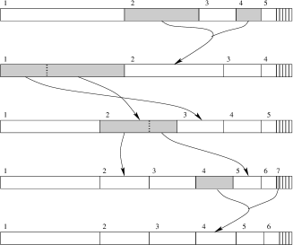
Figure 7: Illustration for the split-merge process. The partition undergoes a merge followed by two splits and another merge.

3.1 Split-merge process

Recall that a partition $\lambda=(\lambda^{(1)},\lambda^{(2)},\dots)$ of the interval $[0,\nu]$ is a sequence of decreasing positive numbers such that $\sum_{i}\lambda^{(i)}=\nu$. Here, $\nu$ is any positive real number. The split-merge process $(\lambda(t):t\geq 0)$, also called coagulation-fragmentation, is a continuous-time stochastic process on partitions where the $i$th and $j$th components ($i\neq j$) merge with rate

$$q_{ij}=2\lambda^{(i)}\lambda^{(j)}/\nu^{2},$$ (26)

and the $i$th component is split uniformly into two parts with rate

$$q_{i}=(\lambda^{(i)})^{2}/\nu^{2}.$$ (27)

Note that the rates are in $[0,1]$ and they add up to $1$, so they can be used directly for the following implementation of the process. If $\lambda{(t)}=(\lambda^{(1)}{(t)},\lambda^{(2)}{(t)},\dots)$ denotes the partition at time $t$, one chooses the new configuration $\lambda{(t+{\rm Exp}(1))}$ after an exponential waiting time with rate $1$ as follows:

• Choose a first part of the partition with probability proportional to its size. That is, the index $i$ is chosen with probability $\lambda^{(i)}{(t)}/\nu$. This is called “size-biased sampling”.

• Choose a second part in the same manner, independently of the first. Let $j$ the corresponding index.

• If $i\neq j$, merge $\lambda^{(i)}{(t)}$ and $\lambda^{(j)}{(t)}$. That is, the partition $\lambda{(t+{\rm Exp}(1))}$ contains all parts $\lambda^{(k)}{(t)}$ with $k\neq i,j$, and a part of size $\lambda^{(i)}{(t)}+\lambda^{(j)}{(t)}$.

• If $i=j$, split $\lambda^{(i)}{(t)}$ uniformly. That is, the partition $\lambda{(t+{\rm Exp}(1))}$ contains all parts $\lambda^{(k)}{(t)}$ with $k\neq i$, and two parts $u\lambda^{(i)}{(t)}$ and $(1-u)\lambda^{(i)}{(t)}$, where $u$ is a uniform random number in $[0,1]$.

• The sequence is rearranged so that $(\lambda^{(k)}{(t+Exp(1))})$ is decreasing.

The process is illustrated in Fig. 7. Additional background can be found in [3, 7]. Tsilevich showed that the Poisson-Dirichlet distribution is invariant for the split-merge process [26]. It was proved in [11] that it is the unique invariant measure (see also [22]).

A key property of our Monte-Carlo process $(\pi_{t}:t\geq 0)$ described in Section 2.4 is that, at each step, either a cycle is split, or two cycles are merged. This is illustrated in Fig. 8. Let us state this precisely.

Figure 8: The transposition $\tau_{xy}$ splits a cycle if $x,y$ belong to the same cycle (left), or it merges two cycles if $x,y$ belong to distinct cycles (right). These are the only two possibilities.

Proposition 3.1

Let $\pi\in{\mathcal{S}}_{\Lambda}$ and $x,y\in\Lambda$ with $x\neq y$.

• If $x,y$ belong to the same cycle in $\pi$, then $x,y$ belong to different cycles in $\pi\circ\tau_{xy}$.

• If $x,y$ belong to different cycles in $\pi$, then $x,y$ belong to the same cycle in $\pi\circ\tau_{xy}$.

See [17] for more details. It is clear that all cycles of $\pi$ that do not involve $x$ or $y$ are also present in $\pi\circ\tau_{xy}$, and reciprocally. The length of the coalesced cycle is equal to the sum of the lengths of the two original cycles, and similarly for a fragmentation.

3.2 Effective split-merge process for macroscopic cycles

We have seen in the previous section that each Monte-Carlo step results in either splitting a cycle, or merging two cycles. We have also seen in Section 2.1 that two kinds of cycles are present: The finite cycles, whose lengths do not diverge in the thermodynamic limit. And the macroscopic cycles, whose lengths are positive fractions of the volume. A Monte-Carlo step does one of the following:

• Merge two finite cycles.

• Merge a macroscopic cycle and a finite cycle.

• Merge two macroscopic cycles.

• Split a finite cycle (resulting in two finite cycles).

• Splits a macroscopic cycle, resulting in a finite and in a macroscopic cycles.

• Splits a macroscopic cycle, resulting in two macroscopic cycles.

One expects each of these options to take place with rates of order $O(1)$ in the limit $|\Lambda|\to\infty$. The ones that are relevant to the effective split-merge process are (c) and (f), since their effect is reflected in a change in $(\lambda^{(1)}(\pi(t)),\lambda^{(2)}(\pi(t)),\ldots)$, the ordered lengths of macroscopic cycles normalized by $|\Lambda|$. Accordingly, we introduce the rate $R_{ij}$ at which the $i$th and $j$th largest cycles merge. It depends on the permutation $\pi$, and, with $i\neq j$, it is given by

$$R_{ij}(\pi)=2\sum_{x\in\gamma^{(i)}}\sum_{y\in\gamma^{(j)}}Q(\pi,\pi\circ\tau_{xy}).$$ (28)

Notice that $R_{ij}(\pi)$ scales to a constant as the volume diverges, since the sum over $x,y$ is of order $|\Lambda|$, and $Q(\cdot)$ is of order $1/|B(\Lambda)|$, see Eq. (19). The rate $R_{i}$ at which the $i$th largest cycle splits into two macroscopic cycles involves the cut-off $K$ that distinguishes finite vs macroscopic cycles:

$$R_{i}(\pi)=\sum_{x\in\gamma^{(i)}}\sum_{k=K}^{L^{(i)}-K}Q(\pi,\pi\circ\tau_{x,\pi^{k}(x)}).$$ (29)

Here, $\pi^{k}(x)$ is the site at “distance” $k$ of $x$ along the cycle $\gamma^{(i)}$. If we set $K=1$ in the right side, we get the rate at which $\gamma^{(i)}$ splits, irrespective of the sizes of the resulting cycles. The expression above gives the rate at which $\gamma^{(i)}$ splits in two cycles, each of which has length greater than $K$. As in previous sections we use the cutoff $K=|\Lambda|^{0.6}$.

We expect that, for almost all permutations in equilibrium, the rates $R_{ij}$ and $R_{i}$ are equal to those of the split-merge process modulo a constant time-scale $R$, resulting from the effective rate of macroscopic processes (c) and (f) above. Recall that $\lambda^{(i)}(\pi)=L^{(i)}(\pi)/|\Lambda|$ is a random variable.

Conjecture 1

Let $T$ such that $\nu_{\infty}(T)>0$. There exists a number $R$ (that depends on $T$ but not on indices) such that for all $i,j$, and all $\varepsilon>0$,

$$\begin{split}&\lim_{|\Lambda|\to\infty}{\mathbb{P}}_{\Lambda}\bigl{(}\bigl{|}R_{ij}-2\lambda^{(i)}\lambda^{(j)}R\bigr{|}>\varepsilon\bigr{)}=0,\\ &\lim_{|\Lambda|\to\infty}{\mathbb{P}}_{\Lambda}\bigl{(}\bigl{|}R_{i}-(\lambda^{(i)})^{2}R\bigr{|}>\varepsilon\bigr{)}=0.\end{split}$$

The time scale of the effective split-merge process is determined by $R$, but the invariant measure is not, so the exact value of $R$ is irrelevant. It is important, however, that it is identical for both the splits and the merges, and for all macroscopic cycles.

Figure 9: Schematic drawing of the situation in a mesoscopic box. It contains finite cycles in light color, and two legs that belong to each of the macroscopic cycles $\gamma$ and $\gamma^{\prime}$. The probability that $\gamma$ and $\gamma^{\prime}$ merge in the next step is proportional to the number of ‘contacts’ between them, which in turn is proportional to $L_{\gamma}L_{\gamma^{\prime}}$. The probability that $\gamma$ splits into two macroscopic cycles is proportional to the self contacts amongst different legs of $\gamma$, which is in turn proportional to $L_{\gamma}^{2}$.

Let us explain the heuristics towards this remarkably simple behavior. Consider a mesoscopic box $\Lambda^{\prime}$ whose size is large enough so that boundary effects are irrelevant, yet small enough so that $\Lambda$ is made up of a large number of mesoscopic boxes. The restriction of $\pi$ on $\Lambda^{\prime}$ gives many finite cycles, and open legs that are parts of macroscopic cycles. See Fig. 9 for a schematic picture. Let us choose a pair of nearest-neighbors $x,y$ at random, with the condition that $x,y$ belong to distinct legs. The probability that $\tau_{xy}$ merges $\gamma^{(i)}$ and $\gamma^{(j)}$ is equal to the probability that $x$ belongs to $\gamma^{(i)}$ and $y$ belongs to $\gamma^{(j)}$, or conversely, which is equal to $2\lambda^{(i)}\lambda^{(j)}/\nu(T)^{2}$, up to vanishing finite-size effects. The probability that $\tau_{xy}$ splits $\gamma^{(i)}$ is equal to the probability that both legs belong to $\gamma^{(i)}$, which is equal to $(\lambda^{(i)}/\nu(T))^{2}$. This heuristics assumes that macroscopic cycles are spread uniformly in space, so they are present in all mesoscopic boxes in proportion to their size, and also that the local configurations do not depend on the situation in other boxes. Note that short range correlations in the cycle structure affect only the probability that a randomly chosen pair $x,y$ belongs to distinct legs, which is absorbed in the constant $R$ that determines the time scale of the effective split merge process.

In addition, we also conjecture that when a cycle is split, it is split uniformly.

Conjecture 2

Let $T$ such that $\nu_{\infty}(T)>0$ and define the CDF for a function of the split length $a\in[0,1]$,

$$\theta_{i}^{(a)}(\pi)=\frac{1}{R_{i}(\pi)}\sum_{x\in\gamma^{(i)}}\sum_{k=K}^{aL^{(i)}}P(\pi,\pi\circ\tau_{x,\pi^{k}(x)})\ .$$ (30)

Then

$$\lim_{|\Lambda|\to\infty}{\mathbb{P}}_{\Lambda}\Bigl{(}\Bigl{|}\theta_{i}^{(a)}(\pi)-a\Bigr{|}>\varepsilon\Bigr{)}=0.$$

If these conjectures hold true, the effective process $\bigl{(}\lambda^{(1)}(\pi(t)),\lambda^{(2)}(\pi(t))\ldots\bigr{)}_{t\geq 0}$ with stationary initial condition converges in the limit $|\Lambda|\to\infty$ to a split-merge process as defined in (26) and (27), running with total rate $R\,\nu_{\infty}^{2}$. Therefore the distribution of cycle lengths has to be invariant with respect to the split-merge process, so it has to be Poisson-Dirichlet. We now check these conjectures numerically.

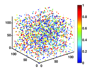
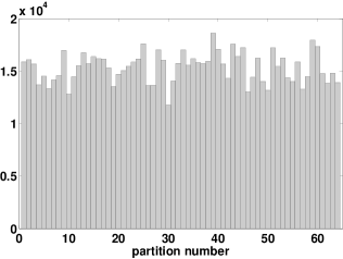
Figure 10: A single permutation has been chosen with respect to the equilibrium measure for $|\Lambda|=128$, $T=0.8$. The longest cycle $\gamma^{(1)}$ is spread everywhere. (Left) Scatter plot of every 500th site along $\gamma^{(1)}$. The color indicates the distance along $\gamma^{(1)}$, renormalized by the length of $\gamma^{(1)}$, starting from the site closest to the origin. (Right) The box $\Lambda$ of volume $128^{3}$ has been partitioned in 64 subsets of volume $32^{3}$. The histogram depicts the number of sites of $\gamma^{(1)}$ that can be found in each subset. It is essentially constant.

3.3 Numerical data about the effective split-merge process

In this section we give numerical evidence that the rates for splitting and merging macroscopic cycles converge to those of a split-merge process, thus confirming the Poisson-Dirichlet distribution of macroscopic cycles. The heuristics behind this argument, as described in the previous section, is that macroscopic cycles are distributed uniformly amongst lattice sites on a mesoscopic level, and not are confined to a bounded region. This is illustrated in Fig. 10.

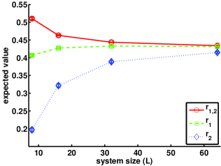
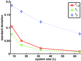
Figure 11: Expectations (left) and standard deviations (right) of the rates defined in (31). $|\Lambda|=8^{3},16^{3},32^{3},64^{3}$, $T=0.8$. The standard error for the mean is within the marker size. Averages were taken over $10^{3}$ realizations.

In order to verify Conjecture 1, the rates of merging the two longest cycles, splitting the longest, and splitting the second longest in the next timestep were calculated using (28) and (29). We define

$$r_{ij}(\pi)=\frac{R_{ij}(\pi)}{2\lambda^{(i)}\lambda^{(j)}}\ ,\qquad r_{i}(\pi)=\frac{R_{i}(\pi)}{(\lambda^{(i)})^{2}}.$$ (31)

Fig. 11 shows that $r_{ij}$ and $r_{i}$ converge to a constant $R$ as expected, supporting Conjecture 1. Note that in addition to convergence of the mean the variance is decreasing, confirming convergence in probability as stated in the conjecture.

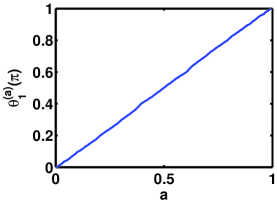
(a) CDF $\theta_{1}^{(a)}(\pi)$

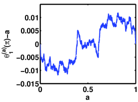
(b) Deviations

Figure 12: Cycles split uniformly. Plot of $\theta_{1}^{(a)}(\pi)$ as defined in (30) for a typical permutation $\pi$ under the equilibrium measure with $|\Lambda|=64^{3}$, $T=0.8$.

If the cycle is split uniformly, $\theta_{i}^{(a)}(\pi)$ as defined in Conjecture 2 is the CDF of a uniform random variable on [0,1]. The graph of $\theta_{1}^{(a)}(\pi)$ is shown in Fig. 12 for a given permutation $\pi$ chosen randomly from the equilibrium measure, which confirms the expected behaviour.

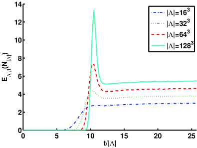
Figure 13: Expected value of the number of cycles longer than $|\Lambda|^{0.6}$, ${\mathbb{E}}_{\Lambda,t}(N_{|\Lambda|})$, as a function of time. The Monte-Carlo chain starts from the identity permutation and has been recorded for various system sizes. Averages were taken over $10^{4}$ realizations.

4 Further prospects

The emergence of macroscopic cycles seems intriguing and it is worth being studied. Starting the Monte-Carlo Markov chain from the identity permutation, one expects the system to display only finite cycles for some time, before infinite objects built up. Let ${\mathbb{E}}_{\Lambda,t}$ denote the corresponding expectation, and $N_{|\Lambda|}(\pi)$ denote the number of cycles of length larger than $|\Lambda|^{0.6}$. Fig. 13 shows ${\mathbb{E}}_{\Lambda,t}(N_{|\Lambda|})$ for $T=0.8$ and various volumes. There is a peak at the transition to the phase with macroscopic cycles. It is certainly due to the presence of many mesoscopic cycles for a short time, that are going to merge afterwards. It would be interesting to get plots for numbers of cycles larger than $|\Lambda|^{a}$ for $a$ other than $0.6$.

While the fraction of sites in large cycles, ${\mathbb{E}}_{\Lambda,t}(\nu)$, varies continuously with time on the scale $t/|\Lambda|$, the steps (c) and (f) of Section 3.2 take place at a very high rate (proportional to $|\Lambda|$) once the phase with macroscopic cycles has been reached. One then expects the lengths of macroscopic cycles to split and merge so fast that the Poisson-Dirichlet distribution appears immediately. The numerical results of Fig. 14 confirms this. Indeed, the expected lengths of the longest cycles, when divided by the number of sites in macroscopic cycles, is equal to the expected values obtained with respect to the Poisson-Dirichlet distribution, that can be found e.g. in [23].

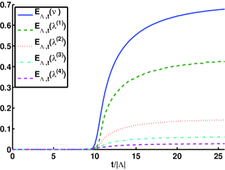
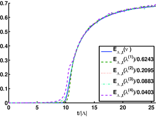
Figure 14: The Poisson-Dirichlet distribution occurs already during equilibration. (a) Expected values of the fraction of sites in macroscopic cycles ${\mathbb{E}}_{\Lambda,t}(\nu)$, and of the lengths of the four largest cycles (divided by the volume). (b) The expectation of the $i$-th longest cycle has been divided by the average length of the $i$-th part in a random partition with Poisson-Dirichlet distribution. It is always close to ${\mathbb{E}}_{\Lambda,t}(\nu)$. $|\Lambda|=128^{3}$, $T=0.8$. Averages were taken over $10^{4}$ realizations.

Finally, let us comment on the physical dimension, taken here to be $d=3$. It is safe to bet that everything is similar in all dimensions greater than 3. On the other hand, the dimension $d=2$ remains mysterious. There are certainly no macroscopic cycles, as was observed in [15]. An open question is whether a phase occurs where a positive fraction of points belong to mesoscopic cycles. This has been ruled out in the “annealed” model that involves averaging over point positions [8, 9]. The present lattice model may be closer to a Bose gas with interactions, on the other hand, where a Kosterlitz-Thouless phase transition is expected. The presence of mesoscopic cycles could indeed be related to the slow decay of correlation functions.

References

- [1] M. Aizenman, Geometric analysis of Fields and Ising models, Commun. Math. Phys. 86, 1–48 (1982)
- [2] M. Aizenman, B. Nachtergaele, Geometric aspects of quantum spin states, Comm. Math. Phys. 164, 17–63 (1994)
- [3] D. Aldous, Deterministic and stochastic models for coalescence (aggregation and coagulation): a review of the mean-field theory for probabilists, Bernoulli 5, 3–48 (1999)
- [4] R. Arratia, A. D. Barbour, S. Tavaré, Logarithmic Combinatorial Structures: A Probabilistic Approach. EMS Monographs in Mathematics (2003)
- [5] N. Berestycki, Emergence of giant cycles and slowdown transition in random transpositions and -cycles, Electr. J. Probab. 16, 152–173 (2011)
- [6] N. Berestycki, R. Durrett Limiting behavior for the distance of a random walk, Electr. J. Probab. 13, 374–395 (2008)
- [7] J. Bertoin, Random Fragmentation and Coagulation Processes. Cambridge University Press (2006)
- [8] V. Betz, D. Ueltschi, Spatial random permutations and infinite cycles, Commun. Math. Phys. 285, 469–501 (2009)
- [9] V. Betz, D. Ueltschi, Spatial random permutations and Poisson-Dirichlet law of cycle lengths, Electr. J. Probab. 16, 1173-1192 (2011)
- [10] N. Crawford, D. Ioffe, Random current representation for transverse field Ising model, Commun. Math. Phys. 296, 447–474 (2010)
- [11] P. Diaconis, E. Mayer-Wolf, O. Zeitouni, M. P. W. Zerner, The Poisson-Dirichlet law is the unique invariant distribution for uniform split-merge transformations, Ann. Probab. 32, 915–938 (2004)
- [12] S. Feng, The Poisson-Dirichlet Distribution and Related Topics. Probability and its Applications, Springer (2010)
- [13] R. P. Feynman, Atomic theory of the transition in Helium, Phys. Rev. 91, 1291–1301 (1953)
- [14] G. Grimmett, Space-time percolation, In “In and out of equilibrium. 2”, Progr. Probab. 60, 305–320 (2008)
- [15] D. Gandolfo, J. Ruiz, D. Ueltschi, On a model of random cycles, J. Statist. Phys. 129, 663–676 (2007)
- [16] C. Goldschmidt, D. Ueltschi, P. Windridge, Quantum Heisenberg models and their probabilistic representations, Entropy and the Quantum II, Contemporary Mathematics 552, 177–224 (2011); arxiv:1104.0983
- [17] J. Kerl, Shift in critical temperature for random spatial permutations with cycle weights, J. Statist. Phys. 140, 56–75 (2010)
- [18] J. F. C. Kingman, Random discrete distributions, J. Roy. Statist. Soc. B 37, 1–15 (1975)
- [19] J. F. C. Kingman, Mathematics of genetic diversity. CBMS-NSF Regional Conference Series in Applied Mathematics, vol. 34, SIAM (1980)
- [20] J. Pitman, M. Yor, The two-parameter Poisson-Dirichlet distribution derived from a stable subordinator, Ann. Probab. 25, 855–900 (1997)
- [21] J. Pitman, Poisson-Dirichlet and GEM invariant distributions for split-and-merge transformations of an interval partition, Combinatorics, Probability and Computing (2002), 11: 501-514
- [22] O. Schramm, Compositions of random transpositions, Israel J. Math. 147, 221–243 (2005)
- [23] L. A. Shepp, S. L. Lloyd, Ordered cycle lengths in a random permutation, Trans. Amer. Math. Soc. 121, 340–357 (1966)
- [24] A. Sütő, Percolation transition in the Bose gas, J. Phys. A 26, 4689–4710 (1993)
- [25] B. Tóth, Improved lower bound on the thermodynamic pressure of the spin Heisenberg ferromagnet, Lett. Math. Phys. 28, 75 (1993)
- [26] N. V. Tsilevich, Stationary random partitions of a natural series, Teor. Veroyatnost. i Primenen. 44, 55–73 (1999)
- [27] D. Wilson, Mixing times of lozenge tiling and card shuffling Markov chains, Ann. Appl. Probab. 14, 274–325 (2004)