Strong quantum violation of the gravitational weak equivalence principle by a non-Gaussian wave-packet

Abstract

The weak equivalence principle of gravity is examined at the quantum level in two ways. First, the position detection probabilities of particles described by a non-Gaussian wave-packet projected upwards against gravity around the classical turning point and also around the point of initial projection are calculated. These probabilities exhibit mass-dependence at both these points, thereby reflecting the quantum violation of the weak equivalence principle. Secondly, the mean arrival time of freely falling particles is calculated using the quantum probability current, which also turns out to be mass dependent. Such a mass-dependence is shown to be enhanced by increasing the non-Gaussianity parameter of the wave packet, thus signifying a stronger violation of the weak equivalence principle through a greater departure from Gaussianity of the initial wave packet. The mass-dependence of both the position detection probabilities and the mean arrival time vanish in the limit of large mass. Thus, compatibility between the weak equivalence principle and quantum mechanics is recovered in the macroscopic limit of the latter. A selection of Bohm trajectories is exhibited to illustrate these features in the free fall case.

I Introduction

In the famous gedanken experiment conceived by Galileo, the universality of the ratio between the gravitational and inertial masses has been studied with test bodies in free fall from the leaning tower of Pisa Ga-book-1638 . Since then several tests of weak equivalence principle have been performed with classical test bodies such as very sensitive pendula or torsion balances establishing extremely accurate conformation of the equality of gravitational and inertial masses. The most familiar tests of the weak equivalence principle are experiments of the Eötvös-type Eo-Math-1890 , which measure the gravitational acceleration of macroscopic objects.Thus Einstein’s weak equivalence principle is established in the Newtonian picture of the gravitational force which is exactly proportional to the inertial mass. The validity of the principle even for quantum mechanical particles is also proved using gravity-induced interference experiments CoOvWe-PRL-1975 ; PeChCh-Nature-1999 .

The traditional equivalence principle is fundamentally both classical and local, and it is interesting to enquire how it is to be understood in quantum mechanics. Principle of equivalence states that inertial mass is equal to gravitational mass; $m_{i}=m_{g}=m$. Another statement is that when all sufficiently small test bodies fall freely, they acquire an equal acceleration independent of their mass or constituent in a gravitational field. Quantum mechanically, it Ho-book-1993 can be said that ” The results of experiments in an external potential comprising just a sufficiently weak, homogeneous gravitational field, as determined by the wave function, are independent of the mass of the system”. The last statement is also known as weak equivalence principle of quantum mechanics (WEQ).

The possibility of violation of weak equivalence principle in quantum mechanics is discussed in a number of papers, for instance using neutrino mass oscillations in a gravitational potential Ga-PRD-1988 . The evidence of violation of WEQ can be shown both experimentally and theoretically. Experimental evidence exists in the interference phenomenon associated with the gravitational potential in neutron and atomic interferometry experiments CoOvWe-PRL-1975 ; PeChCh-Nature-1999 . Theoretically, for a particle bound in an external gravitational potential, it is seen that the radii, frequencies and binding energy depend on the mass of the bound particle Gr-RMP-1979 ; Gr-AP-1968 ; Gr-RMP-1983 .

The free fall of test particles in a uniform gravitational field in the case of quantum states with and without a classical analogue was re-examined by Viola and OnofrioVi-PRD-1997 . Another quantum mechanical approach of the violation of WEQ was given by Davies Da-CQG-2004 for a quantum particle in a uniform gravitational field using a model quantum clock Pe-AJP-1980 . A quantum particle moving in a gravitational field can penetrate the classically forbidden region beyond the classical turning point of the gravitational potential and the tunnelling depth depends on the mass of the particle. So, there is a small mass-dependent quantum delay in the return time representing a violation of weak equivalence principle. This violation is found within a distance of roughly one de Broglie wavelength from the turning point of the classical trajectory.

In the recent past, Ali et al. Al-CQG-2006 have shown an explicit mass dependence of the position probabilities for quantum particles projected upwards against gravity around both the classical turning point and the point of initial projection using Gaussian wave packet. They also have shown an explicit mass dependence of the mean arrival time at an arbitrary detector location for a Gaussian wave packet under free fall. Thus both the position probabilities and the mean arrival time show the violation of WEQ for quantum particles represented by Gaussian wave packets. In the present paper, using a class of non-Gaussian wave packets involving a tunable parameter, we shall compute position detection probabilities around the classical turning point and the point of initial projection and also compute the mean arrival time for atomic and molecular mass particles represented by non-Gaussian wave packets to observe stronger violation of WEQ for quantum particles. To compute the mean arrival time, we consider the case when the particles are dropped from a height with zero initial velocity.

Violation of WEQ arises as a consequence of the spread of wave packets the magnitude of which itself depends on the mass. In order to illustrate this effect we present an analysis in terms of Bohmian trajectories. In the Bohmian model Bo-PR-1952 each individual particle is assumed to have a definite position, irrespective of any measurement. The pre-measured value of position is revealed when an actual measurement is done. Over an ensemble of particles having the same wave function $\psi$, these ontological positions are distributed according to the probability density $\rho=|\psi|^{2}$ where the wave function $\psi$ evolves with time according to the Schrödinger equation and the equation of motion of any individual particle is determined by the guidance equation $v=J/\rho$, where $v$ is the Bohmian velocity of the particle and $J$ is the probability current density. Solving the guidance equation one gets the trajectory of the particle. In the present work we describe the evolution of Bohmian trajectories in terms of the mass and the tunable parameter of the non-Gaussian wave packet.

II Position Detection Probability

Let us consider an ensemble of quantum particles projected upwards against gravity with a given initial mean position and mean velocity. Our motivation is to look for greater violation of the equivalence principle compared to that achieved by a Gaussian wave packet. Hence, we formulate a one-dimensional non-Gaussian wave function which represents the initial state of each particle, given by

$$\psi(z,t=0)=N\left[1+\alpha\sin{\left(\frac{\pi}{4\sigma_{0}}z\right)}\right]e^{-\frac{z^{2}}{4\sigma_{0}^{2}}+ik_{0}z}$$ (1)

Here, $\alpha$ is the tuneable parameter varying from $0$ to $1$. The normalisation factor $N$ is given by

$$N = \left(\sqrt{2\pi}\sigma_{0}\left[1+\frac{\alpha^{2}}{2}\>(1-e^{-\pi^{2}/8})\right]\right)^{-1/2}~{}.$$ (2)

The salient features corresponding to the above wave packet are its asymmetry, its infinite tail, and its reduciblity to a Gaussian wave packet upon a continuous decrement of the parameter $\alpha$ to zero. The property of an infinite tail of the above wave function is not associated with non-Gaussian forms that are generated by truncating the Gaussian distribution. The asymmetry of the wave packet (due to the sine function) entails a difference between its mean and peak, as will be further evident in our following analysis.

The initial group velocity is given by $u=\frac{\hbar k_{0}}{m}$, where $m$ is the mass of the particle and $k_{0}$ is the wave number. For $\alpha=0$, we get the Gaussian wave function. If $\psi_{1}$ and $\psi_{2}$ represent the initial wave functions for particles 1 and 2 in the Schrödinger picture, then the mean initial conditions are

$$\langle\hat{z}\rangle_{\psi_{1}}=\langle\hat{z}\rangle_{\psi_{2}}=\langle\hat{z}(0)\rangle\;,$$

$$\frac{\langle\hat{p}_{z}\rangle_{\psi_{1}}}{m_{1}}=\frac{\langle\hat{p}_{z}\rangle_{\psi_{2}}}{m_{2}}=u$$ (3)

where $\langle\hat{z}\rangle_{\psi}$ and $\langle\hat{p}_{z}\rangle_{\psi}$ represent the expectation values for position and momentum operators respectively. Here, we have restricted ourselves to a one-dimensional representation along the vertical $z$ direction for simplicity. With the propagator

$$G(z,t|y,0)=\sqrt{\frac{m}{2\pi i\hbar t}}e^{\frac{im}{2\hbar t}(z-y)^{2}-\frac{imgt}{2\hbar}(z+y)-\frac{img^{2}t^{3}}{24\hbar}}$$ (4)

of a particle in the linear gravitational potential $V=mgz$ and with the relation

$$\psi(z,t)=\int dyG(z,t|y,0)\psi(y,0)$$ (5)

one can get the Schrödinger time evolved wave function $\psi(z,t)$ at any subsequent time $t$ as

$$\psi(z,t) = N\sqrt{\frac{\sigma_{0}}{s_{t}}}~{}e^{\frac{im}{2\hbar t}[z^{2}-gt^{2}z-\frac{g^{2}t^{4}}{12}]}$$ (6)

$$\times \left[e^{-\frac{im}{2\hbar t}\frac{\sigma_{0}}{s_{t}}[z-\frac{\hbar t}{m}k_{0}+\frac{gt^{2}}{2}]^{2}}+\frac{\alpha}{2i}e^{-\frac{im}{2\hbar t}\frac{\sigma_{0}}{s_{t}}[z-\frac{\hbar t}{m}(k_{0}+\beta)+\frac{gt^{2}}{2}]^{2}}-\frac{\alpha}{2i}e^{-\frac{im}{2\hbar t}\frac{\sigma_{0}}{s_{t}}[z-\frac{\hbar t}{m}(k_{0}-\beta)+\frac{gt^{2}}{2}]^{2}}\right]$$

where, $s_{t}=\sigma_{0}\left(1+i\frac{\hbar t}{2m\sigma_{0}^{2}}\right)$ and $\beta=\frac{\pi}{4\sigma_{0}}$. The probability density is given by

$$\rho(z,t) = |\psi(z,t)|^{2}=N^{2}\frac{\sigma_{0}}{\sigma_{G}}e^{E_{1}}\left[e^{E_{2}}+\alpha\left(e^{E_{3}}\sin{A_{1}}+e^{E_{4}}\sin{A_{2}}\right)+\frac{\alpha^{2}}{4}\left(1+e^{E_{5}}-2e^{E_{6}}\cos{A_{3}}\right)\right]~{},$$ (7)

where

$$E_{1} = -\frac{\left[\pi\hbar t+4m\sigma_{0}\left(z-ut+\frac{1}{2}gt^{2}\right)\right]^{2}}{32m^{2}\sigma_{G}^{2}\sigma_{0}^{2}}~{},$$

$$E_{2} = \frac{\pi\hbar t\left[\pi\hbar t+8m\sigma_{0}\left(z-ut+\frac{1}{2}gt^{2}\right)\right]}{32m^{2}\sigma_{G}^{2}\sigma_{0}^{2}}~{},$$

$$E_{3} = \frac{\pi\hbar t\left[\pi\hbar t+24m\sigma_{0}\left(z-ut+\frac{1}{2}gt^{2}\right)\right]}{64m^{2}\sigma_{G}^{2}\sigma_{0}^{2}}~{},$$

$$E_{4} = \frac{\pi\hbar t\left[\pi\hbar t+8m\sigma_{0}\left(z-ut+\frac{1}{2}gt^{2}\right)\right]}{64m^{2}\sigma_{G}^{2}\sigma_{0}^{2}}~{},$$

$$E_{5} = \frac{\pi\hbar t\left(z-ut+\frac{1}{2}gt^{2}\right)}{2m\sigma_{G}^{2}\sigma_{0}}~{},$$

$$E_{6} = \frac{E_{5}}{2}~{},$$

$$A_{1} = \frac{\pi\left[-\pi\hbar t+8m\sigma_{0}\left(z-ut+\frac{1}{2}gt^{2}\right)\right]}{32m\sigma_{G}^{2}}~{},$$

$$A_{2} = \frac{\pi\left[\pi\hbar t+8m\sigma_{0}\left(z-ut+\frac{1}{2}gt^{2}\right)\right]}{32m\sigma_{G}^{2}}~{},$$

$$A_{3} = \frac{\pi\sigma_{0}\left(z-ut+\frac{1}{2}gt^{2}\right)}{2\sigma_{G}^{2}}~{},$$

and

$$\sigma_{G} = |s_{t}|=\sigma_{0}\left(1+\frac{\hbar^{2}t^{2}}{4m^{2}\sigma_{0}^{4}}\right)^{\frac{1}{2}}~{},$$ (8)

is the spreading of the Gaussian wave packet. The probability density is explicitly mass dependent. Here, the spreading of the wave packet is given by

$$\sigma_{NG} = \frac{\sqrt{\lambda^{(0)}+\lambda^{(2)}\alpha^{2}+\lambda^{(4)}\alpha^{4}}}{4m\sigma_{0}\left[2e^{\frac{\pi^{2}}{8}}+\alpha^{2}\left(e^{\frac{\pi^{2}}{8}}-1\right)\right]}$$ (9)

where,

$$\lambda^{(0)} = 64e^{\frac{\pi^{2}}{4}}m^{2}\sigma_{0}^{2}\sigma_{G}^{2}~{},$$

$$\lambda^{(2)} = 8e^{\frac{\pi^{2}}{8}}\pi^{2}m^{2}\sigma_{0}^{4}\left(1-2e^{\frac{\pi^{2}}{16}}\right)+64e^{\frac{\pi^{2}}{8}}m^{2}\sigma_{0}^{2}\sigma_{G}^{2}\left(-1+e^{\frac{\pi^{2}}{8}}\right)+2e^{\frac{\pi^{2}}{4}}\pi^{2}\hbar^{2}t^{2}~{},$$

$$\lambda^{(4)} = \left(e^{\frac{\pi^{2}}{8}}-1\right)\left[16m^{2}\sigma_{0}^{2}\sigma_{G}^{2}\left(e^{\frac{\pi^{2}}{8}}-1\right)+4\pi^{2}m^{2}\sigma_{0}^{4}+e^{\frac{\pi^{2}}{8}}\pi^{2}\hbar^{2}t^{2}\right]~{}.$$ (10)

which is also mass dependent.

Fig. 1 gives the plot of $\sigma_{NG}$ vs $\alpha$.

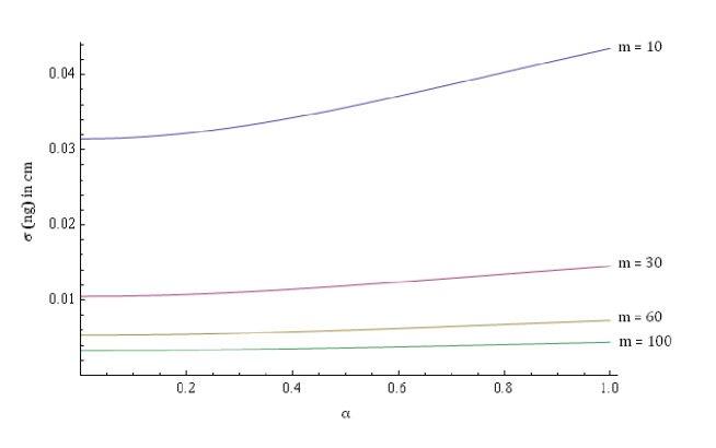
Figure 1: The variation of the width of the wave packet with $\alpha$ for different constant values of $m$ (in a.m.u.). We take $\sigma_{0}=10^{-3}$ cm, $t=1$ sec and $u=10^{3}$ cm $s^{-1}$.

From this figure, we can see that for large masses, $\sigma_{NG}$ becomes almost constant with $\alpha$. For a particular value of $\alpha$, $\sigma_{NG}$ decreases with increasing value of mass $m$.

The expression for expectation value of z is given by

$$\langle z\rangle=\frac{\pi\alpha\sigma_{0}}{2+\alpha^{2}\left(1-e^{-\frac{\pi^{2}}{8}}\right)}\,e^{-\frac{\pi^{2}}{32}}+ut-\frac{1}{2}gt^{2}$$ (11)

Ehrenfest’s theorem states that expectation value of quantum mechanical operators obey classical laws of motion, the instances of which are given below

$$\frac{d\langle z\rangle}{dt}=\frac{\langle p\rangle}{m},$$

$$\frac{d\langle p\rangle}{dt}=\langle-\frac{\partial V}{\partial z}\rangle.$$ (12)

It is possible to check that Ehrenfest’s theorem is satisfied for our non-Gaussian wave packet. In the Gaussian limit (i.e., $\alpha\rightarrow 0$), $\langle z\rangle=z_{peak}$ and the dynamics of $\langle z\rangle$ is like a classical point particle, as expected.

In Eq. (11) the first term is $\alpha$-dependent. There is no $m$ in this expression. So, $\langle z\rangle$ is $\alpha$-dependent but mass independent. With the solutions obtained from the equation $\frac{d|\psi|^{2}}{dz}=0$, we can get the value of $z_{peak}$ for which $|\psi|^{2}$ is maximum. But the equation can’t be solved analytically. So, we have computed $z_{peak}$ numerically. $z_{peak}$ depends both on $\alpha$ and mass. In Table 1, it is shown numerically how $z_{peak}$ and $\langle z\rangle$ vary with $\alpha$, for $0\leq\alpha\leq 1$. In Table 2, it is shown numerically how those two vary with mass. It is clear that $z_{peak}\neq\langle z\rangle$ and $z_{peak}$ increases with $\alpha$ and mass $m$ but $\langle z\rangle$ increases with $\alpha$, and remains constant for all masses.

Fig. 2 shows the variation of $z_{peak}$ and $\langle z\rangle$ with time simultaneously. Dotted curve shows the motion of $z_{peak}$ whereas the continuous curve shows the motion of $\langle z\rangle$. As we take $\sigma_{0}=10^{-7}$ cm, the $\alpha$-dependence of $\langle z\rangle$ and $z_{peak}$ becomes vanishingly small. So, this $\alpha$-dependence can not be shown graphically. As a result, the curves for $z_{peak}$ and $\langle z\rangle$ coincide totally in this graph.

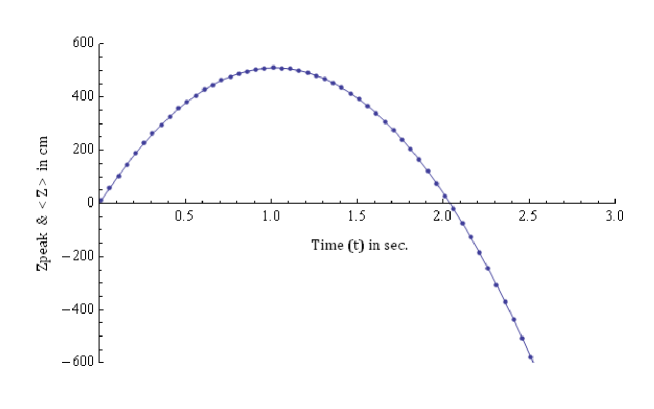
Figure 2: The variation of $z_{peak}$ and $\langle z\rangle$ with time $t$. We take $\sigma_{0}=10^{-7}$ cm, $u=10^{3}$ cm $s^{-1}$, $m=50$ a.m.u. and $\alpha=0.5$.

Table 1: The variation of $\langle z\rangle$ and $z_{peak}$ in cm with $\alpha$ for mass $m=10$ a.m.u. $t=2$ sec and $\sigma_{0}=0.1$ cm.

$\alpha$	$z_{peak}$	$\langle z\rangle$
	in cm	in cm
0	38.59999999999815	38.599999999999910
0.1	38.61540633397262	38.611498366598200
0.2	38.62925626009014	38.622755653868810
0.3	38.64090000000000	38.633500000000000
0.4	38.65026513575232	38.643679695976970
0.5	38.65786585282045	38.652999876917650
0.6	38.66400000000000	38.661400000000000
0.7	38.66910000000000	38.668800000000000
0.8	38.67337906376510	38.675246198243485
0.9	38.67696171641449	38.680689435211890
1.0	38.68002216630916	38.685197660661515

Table 2: The variation of $\langle z\rangle$ and $z_{peak}$ in cm with mass $m$ in a.m.u. for $\alpha=0.5$, $t=2$ sec and $\sigma_{0}=0.1$ cm.

Mass $(m)$	$z_{peak}$	$\langle z\rangle$
in a.m.u.	in cm	in cm
30	38.657865898827980	38.65299987691765
60	38.657865903136155	38.65299987691765
90	38.657865903934166	38.65299987691765
120	38.657865904213070	38.65299987691765
150	38.657865904342295	38.65299987691765

Now, we want to observe the expression for $\langle z\rangle$ in the classical limit. If a full classical description is to emerge from quantum mechanics, we must be able to describe quantum systems in phase-space. The Wigner distribution function Wi-PR-1932 ; FoCo-AJP-2002 which is one of the phase-space distributions, can provide a re-expression of quantum mechanics in terms of classical concepts.

The Wigner distribution function which is calculated from the time evolved wave function $\psi(z,t)$, is given by

$$D_{w}(z,p,t)=\frac{1}{\pi\hbar}\int_{-\infty}^{\infty}\psi^{*}(z+y,t)\psi(z-y,t)e^{\frac{2ipy}{\hbar}}dy$$ (13)

and the marginals of which yield the correct quantum probabilities for position and momentum separately.

By substituting the value of $\psi^{*}(z+y,t)$ and $\psi(z-y,t)$ using Eq.(5) we obtain the Wigner distribution function $D_{w}(z,p,t)$ for non-Gaussian wave packet. It satisfies the classical Liouville’s equation DaSe-CS-2002 given by

$$\frac{\partial D_{w}(z,p,t)}{\partial t}+\dot{z}\frac{\partial D_{w}(z,p,t)}{\partial z}+\dot{p}\frac{\partial D_{w}(z,p,t)}{\partial p}=0$$ (14)

Here, $\dot{z}=p/m$ and $\dot{p}=-mg$ are obtained from Hamilton’s equation of motion given by

$$\dot{z}=\frac{\partial H}{\partial p},$$

$$\dot{p}=-\frac{\partial H}{\partial z}$$

where, $H=p^{2}/2m+mgz$ is the Hamiltonian of the system.

The corresponding position distribution function is given by

$$\rho_{C}(z,t)=\int_{-\infty}^{\infty}D_{w}(z,p,t)dp.$$ (16)

So, the expression for the average value of $z$ using Wigner distribution function is given by

$$\langle z\rangle = \frac{\int_{-\infty}^{\infty}z\rho_{C}(z,t)dz}{\int_{-\infty}^{\infty}\rho_{C}(z,t)dz}$$ (17)

$$= \frac{\pi\alpha\sigma_{0}}{2+\alpha^{2}\left(1-e^{-\frac{\pi^{2}}{8}}\right)}\,e^{-\frac{\pi^{2}}{32}}+ut-\frac{1}{2}gt^{2}\equiv z_{0}+ut-\frac{1}{2}gt^{2}$$

which is exactly equal to the quantum mechanical expectation value of $z$.

The particles are projected upwards against gravity. Cassicaly, the refrence point $z=0$ reaches the maximum height $z=z_{max}=ut_{1}-\frac{1}{2}gt_{1}^{2}$ at the time $t=t_{1}=u/g$. So, the probability of finding the particles $P_{1}(m)$ within a very narrow detector region $(-\>\epsilon\>to\>+\>\epsilon)$ around $z_{max}$ is given by

$$P_{1}(m)=\int_{z_{max}-\epsilon}^{z_{max}+\epsilon}|\psi(z,t_{1})|^{2}dz.$$ (18)

At a later time $t=t_{2}=2u/g$, the classical peak of the wave packet returns to it’s initial projection point at $z=0$. Similarly, the probability of finding the particles $P_{2}(m)$ within a very narrow detector region $(-\>\epsilon\>to\>+\>\epsilon)$ around $z=0$ is given by

$$P_{2}(m)=\int_{-\epsilon}^{+\epsilon}|\psi(z,t_{2})|^{2}dz.$$ (19)

From Fig. 3 and Fig. 4, it is clear that both the probabilities are mass dependent for an initial non-Gaussian position distribution for smaller masses. This effect of mass dependence of the probabilities occur essentially as the spreading of the wave packet under linear gravitational potential depends on the mass of the particles. These probabilities become saturated in the limit of large mass. As $\alpha$ increases, both the probabilities decrease for a particular value of $m$. The departure from the result for the Gaussian ($\alpha=0$) case increases with the value of the non-Gaussian parameter, signifying a stronger violation of the weak equivalence principle.

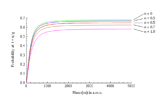
Figure 3: The variation of probability $P_{1}(m)$ with mass (in a.m.u.) for different constant values of $\alpha$. We take $u=10^{3}$ cm $s^{-1}$, $\sigma_{0}=10^{-3}$ cm and $\epsilon=\sigma_{0}$.

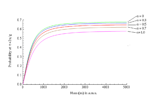
Figure 4: The variation of probability $P_{2}(m)$ with mass (in a.m.u.) for different constant values of $\alpha$. We take $u=10^{3}$ cm $s^{-1}$, $\sigma_{0}=10^{-3}$ cm and $\epsilon=\sigma_{0}$.

III Mean Arrival Time

Now, Let us consider the quantum particles subjected to free fall from the initial position at $z=0$ under gravity with the initial state given by Eq.(1) and with $u=0$. Using the probability current approach prob the mean arrival time of the quantum particles to reach a detector location at $z=Z$ is given by

$$\bar{\tau}=\frac{\int_{0}^{\infty}|J(z=Z,t)|\,t\,dt}{\int_{0}^{\infty}|J(z=Z,t)|\,dt}\\$$ (20)

where, $J(z,t)$ is the quantum probability current density. However, we emphasize that the definition of the mean arrival time used in the above equation is not a uniquely derivable result within standard quantum mechanics. It should also be noted that $J(z,t)$ can be negative, so we take the modulus sign in order to use the above definition. From Eq.(20), it can be seen that the integral of the denominator converges whereas the integral of the numerator diverges formally. To avoid this problem, several techniques have been employed DaEgMu-quant-2001 . In this paper, to obtain convergent results of the numerator we use the simple technique of getting a cut-off at $t=T$ in the upper limit of the time integral with $T=\sqrt{2(|Z|+3\sigma_{T})/g}$. $\sigma_{T}$ is the width of the wave packet at time $T$. Thus, our calculations of the arrival time are valid upto the $3\sigma_{T}$ level of spread in the wave function.

Here, the expression for the Schrödinger probability current density $J(z,t)$ with the initial non-Gaussian position distribution is given by

$$J(z,t) = \frac{\hbar}{m}\Im{(\psi^{*}\nabla\psi)}=N^{2}\frac{e^{E_{1}}}{32m^{2}\sigma_{0}\sigma_{G}^{3}}\left(\eta^{(0)}+\alpha\eta^{(1)}+\alpha^{2}\eta^{(2)}\right)~{},$$ (21)

where

$$\eta^{(0)} = 8e^{E_{2}}\left[\hbar^{2}t\left(z-\frac{1}{2}gt^{2}\right)+4m^{2}\sigma_{0}^{4}\left(u-gt\right)\right]~{},$$

$$\eta^{(1)} = \eta^{(0)}e^{-E_{2}}\left(e^{E_{3}}\sin{A_{1}}+e^{E_{4}}\sin{A_{2}}\right)-2\pi\hbar^{2}t\sigma_{0}\left(e^{E_{3}}\cos{A_{1}}+e^{E_{4}}\cos{A_{2}}\right)+4\pi m\hbar\sigma_{0}^{3}\left(e^{E_{3}}\sin{A_{1}}-e^{E_{4}}\sin{A_{2}}\right)~{},$$

$$\eta^{(2)} = \left[2\hbar^{2}t\left(z-\frac{1}{2}gt^{2}\right)+8m^{2}\sigma_{0}^{4}\left(u-gt\right)\right](1+e^{E_{5}}-2e^{E_{6}}\cos{A_{3}})-2\pi\hbar^{2}t\sigma_{0}e^{E_{6}}\sin{A_{3}}+2\pi m\hbar\sigma_{0}^{3}(-1+e^{E_{5}})~{},$$

and where the $E_{i}$’s are defined below Eq.(7).

It is clear that $J(z,t)$ is explicitly mass dependent. So, $\bar{\tau}$ is also mass dependent. From Fig. 5, we can observe that for smaller masses $\bar{\tau}$ is mass dependent and for larger masses it becomes mass independent. For a particular value of mass, $\bar{\tau}$ increases with $\alpha$.

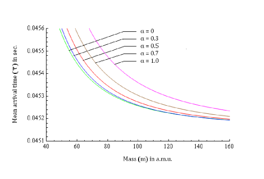
Figure 5: The variation of mean arrival time with mass (in a.m.u.) for different constant values of $\alpha$. We take $\sigma_{0}=10^{-6}$ cm, $Z=-1$cm and $u=0$.

From Fig. 6, we can see that for large masses, $\bar{\tau}$ becomes almost constant with $\alpha$. For a particular value of $\alpha$, $\bar{\tau}$ decreases with increasing value of mass $m$.

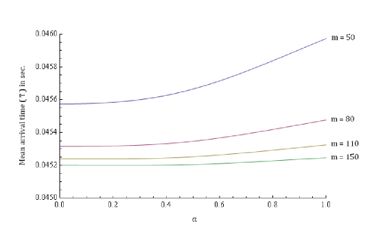
Figure 6: The variation of mean arrival time with $\alpha$ for different constant values of $m$ (in a.m.u.).We take $\sigma_{0}=10^{-6}$ cm, $Z=-1$cm and $u=0$.

It is clear that the mass-dependence of the mean arrival time gradually vanishes as the mass is increased. Thus, compatibility with the equivalence principle emerges in the limit of large mass, or classical limit. Note that with the increase of the parameter $\alpha$, one needs to go to higher values of mass in order for the mass-dependence to become insignificant. Thus, a non-Gaussian wave packet can exhibit non-classical features in a mass range where its Gaussian counterpart behaves classically.

IV Bohm Trajectory Approach

Within the Bohmian interpretation of quantum mechanics Bo-PR-1952 each individual particle is assumed to have a definite position, irrespective of any measurement. The equation of motion of the particle is,

$$m\ddot{\vec{x}} = -\nabla(V+Q)|_{\vec{x}=\vec{x}(t)}~{},$$ (22)

where $Q=-\frac{\hbar^{2}}{2m}\frac{\nabla^{2}\sqrt{\rho}}{\sqrt{\rho}}$ is called ’quantum potential energy’ and it is explicitly mass-dependent and $\vec{x}(t)$ determines the path of the particle. In the gravitational potential $V=mgz$ the quantum version of Newton’s second law is given by

$$\ddot{z} = g-\frac{1}{m}\frac{\partial Q}{\partial z}\bigg{|}_{z=z(t)}~{}.$$ (23)

To quote from Holland Ho-book-1993 , ”It is immediately clear that the assumption of the equality of the inertial and passive gravitational masses does not imply that all bodies fall with an equal acceleration in a given gravitational field, due to the intervention of the mass-dependent quantum force term.” Thus, WEQ is violated. The arrival-time problem is unambiguously solved in the Bohmian mechanics, where for an arbitrary scattering potential $V(\vec{x})$, one finds Le-book-2002 that for those particles that actually reach $\vec{x}=\vec{X}$, the arrival-time distribution is given by the modulus of the probability current density, i.e., $|J(\vec{X},T)|$.

The quantum potential $Q$ is nonlocal, and thus it is expected that its effect on the violation of WEQ is manifested in a way similar to the violation observed as a consequence of the spread of the wave packet. We compute a set of Bohmian trajectories corresponding to free fall of our non-Gaussian wave packet with the tunable parameter $\alpha$. Fig. 7 shows a selection of Bohmian trajectories exhibiting their spread depending upon the values of $m$ and $\alpha$. Note that for small mass, the trajectories with initial positions on the left and right of the center of the wave packet (mean $\langle z\rangle$) spread out with evolution, indicating violation of WEQ. The magnitude of spread increases with $\alpha$, signifying stronger violation of WEQ with increased departure from Gaussianity. The spread of the trajectories decreases as mass is increased, leading to the emergence of WEQ in the classical limit.

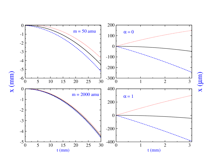
Figure 7: A selection of Bohmian trajectories for $u=0$ (free fall) and $\sigma_{0}=10^{-6}$cm. In the left column tunable parameter $\alpha$ has the fixed value $\alpha=0.5$ and in the right one mass is constant and equal to $m=100~{}$amu. The solid black trajectory starts at $\langle z\rangle(0)$ , the dashed blue one at $\langle z\rangle(0)-2\sigma_{0}$ and the dotted red one at $\langle z\rangle(0)+2\sigma_{0}$.

V Conclusions

To summarize, in this work we have studied the violation of the gravitational weak equivalence principle in quantum mechanics using a non-Gaussian wave packet. The wave packet is constructed in such a way, that its departure from Gaussianity is represented by a continuous and tunable parameter $\alpha$. The asymmetry of the wave packet entails a difference between its mean and peak, and causes the peak to evolve differently from a classical point particle, whereas the mean evolves like a classical point particle modulo a constant depending upon the parameter $\alpha$. Such a result is consistent with the Ehrenfest therorem, as we have shown, and re-confirmed using the Wigner distribution. The correspondence with the results following from a Gaussian wave packet is achieved in the limit of $\alpha\to 0$.

The weak equivalence principle is shown to be violated first through the dependence on mass of the position detection probabilities of freely falling particles. The magnitude of violation increases with the increase of the non-Gaussian parameter $\alpha$, signifying stronger viotation of WEQ with larger deviation from Gaussianity. We next compute the arrival time of freely falling wave packets through the probability current distribution corresponding to the non-Gaussian wave packet. The violation of WEQ is again exhibited with the dependence on mass of the mean arrival time. It is observed that in the limit of large mass the classical value for the mean arrival time is approached, thereby indicating the emergence of the WEQ in the classical limit. In this context it is worthwhile to mention that though our work follows as a natural consequence of quantum mechanics or quantum theory in the non-relativistic limit, it does not imply a violation of general covariance in the relativistic domain. An interesting connection between the non-relativistic limit of quantum theory and the principle of equivalence has recently been discussed PaPa-PRD-2011 . Finally, a computation of Bohmian trajectories further establishes the stronger violation of WEQ by a non-Gaussian wave packet. We conclude by noting that realization of exactly Gaussian wave packets is rather difficult in real experiments. One of the consequences of our results is to enable relaxation of the wave packet to be Gaussian, and therefore it can facilitate the experimental observation of the violation of WEQ, as well as enable a quantitative verification of the way the violation of WEQ depends on the departure from the Gaussian nature of the wave packet. Other ramifications of this result call for further study.

Acknowledgements: PC, DH, ASM and SS acknowledge support from DST India Project no. SR/S2/PU-16/2007. MRM and SVM acknowledge finantial support of the University of Qom.

References

- (1) Galilei G 1638 Discorsi Intorno a due Nuove Scienze(Leiden: Elsevier) (English translation edited by H Crew and A de Salvio (New York: Macmillan 1914) pp 212-3)
-
(2)
Eötvös R V Math. Nat. Ber. Ungarn. 8 65 (1890);
R. V. Eötvös, V. Pekar, and E. Fekete, Ann. Phys. (N.Y.) 68 11 (1922). - (3) Colella R, Overhauser A W and Werner S A Phys. Rev. Lett. 34 1472 (1975).
- (4) Peters A, Chung K Y and Chu S, Nature 400 849 (1999).
- (5) Holland P 1993 The Quantum Theory of Motion (London: Cambridge University Press) pp 259-66.
-
(6)
Gasperini M, Phys. Rev. D 38 2635 (1988);
Krauss L M and Tremaine S Phys. Rev. Lett. 60 176 (1988);
Halprin A and Leung C N Phys. Rev. D 53 5365 (1996);
Mureika J R Phys. Rev. D 56 2408 (1997);
Gago A M, Nunokawa H and Funchal R Z Phys. Rev. Lett. 84 4035 (2000);
Adunas G Z, Milla E R and Ahluwalia D V Gen. Rel. Grav. 33 183 (2001). - (7) Greenberger D M and Overhauser A W 1979 Rev. Mod. Phys. 51 43
- (8) Greenberger D M 1968 Ann. Phys. 47 116
- (9) Greenberger D M 1983 Rev. Mod. Phys. 55 875
- (10) Viola L and Onofrio R 1997 Phys. Rev. D 55 455
- (11) Davies P C W 2004 Class. Quantum Grav. 21 2761
- (12) Peres A 1980 Am. J. Phys. 48 552
- (13) Ali M A, Majumdar A S, Home D and Pan A K (2006) Class. Quantum Grav. 23 6493
-
(14)
Bohm D 1952 Phys. Rev. 85 166;
Bohm D 1952 Phys. Rev. 85 180;
Bohm D 1953 Phys. Rev. 89 458 - (15) Wigner E 1932 Phys. Rev. 40 749
-
(16)
Ford G W and O’Connell R F 2002 Am. J. Phys. 70 319;
Robinett R W, Doncheski M A and Bassett L C 2005 Preprint quant-ph/0502097 - (17) Das S K and Sengupta S 2002 Current Science 83 1234
- (18) Dumont R S and Marchioro T L II 1993 Phys. Rev. A 47 85; Leavens C R 1993 Phys Lett A 178 27
-
(19)
Damborenea J A, Egusquiza I L and Muga J G 2001 Preprint quant-ph/0109151;
Hahne G E 2003 J. Phys. A: Math. Gen. 36 7149 -
(20)
Leavens C R 2002 Bohm trajectory approach to timing electrons Time in Quantum Mechanics ed J G Muga, R Sala and I L Egusquiza (Berlin: Springer);
Leavens C R 1993 Phys. Lett. A 178 27;
Leavens C R 1996 The ‘tunneling-time problem’ for electrons Bohmian Mechanics and Quantum Theory: An Appraisal ed J Cushing, A Fine and S Goldstein (Dordrecht: Kluwer Academic) p 111;
Leavens C R 1998 Phys. Rev. A 58 840 - (21) Padmanabhan H and Padmanabhan T 2011 Phys. Rev. D 84 085018