Influence of the atomic-wall collision elasticity on the coherent population trapping resonance shape

Abstract

We studied theoretically a coherent population trapping resonance formation in cylindrical cell without buffer gas irradiated by a narrow laser beam. We take into account non-zero probabilities of elastic (“specular”) and inelastic (“sticking”) collision between the atom and the cell wall. We have developed a theoretical model based on averaging over the random Ramsey pulse sequences of times that atom spent in and out of the beam. It is shown that the shape of coherent population trapping resonance line depends on the probability of elastic collision.

1 Introduction

In the simplest case, the coherent population trapping (CPT) effect appears in three-level $\Lambda$-system, see figure 1. The atom is interacting with a two-frequency laser field coupling two metastable states with a short-living state. When the frequency difference between the laser field components is equal to the frequency of the transition between two metastable states (two-photon resonance conditions), the “dark state” that does not interact with the laser field appears. This “dark state” is the coherent superposition of the metastable states. If one scans the frequency difference of two laser components near the two-photon resonance, one observes the CPT resonance, an abrupt decrease of the fluorescence intensity [1, 2, 3]. CPT phenomenon allows to create a window in the absorption spectrum [4]. This effect is used in compact frequency standard [5, 6], the stimulated adiabatic passage technique of population transfer between the states of atoms and molecules [7], laser cooling [8] and magnetic field measurements [9, 10].

It is well known [11, 12, 13, 14, 15, 16, 17, 18, 19] that the CPT resonance shape is affected by the movement of atoms between the beam zone illuminated by the laser radiation and the dark zone. The theory of the CPT resonance formation in wall-coated cells without buffer gas based on averaging over random Ramsey sequences of times which the active atom spent in the bright and dark zones was developed in [12, 13, 14]. In these models, it was assumed that in any atomic-wall collision the atom sticks to the cell wall for some time. During this time atom exchanges its kinetic energy with the cell wall and then it is released back to the cell volume with alternated velocity that is not correlated with atomic velocity before the collision. Atoms make many transitions between these two zones during the lifetime of metastable states coherence. This cohrerence is assumed to be preserved in the collision [20].

Assumption about sticking collisions is based on the studies of relaxation of polarization in Rubidium vapors in paraffin-coated cell performed by Bouchiat and Brossel [21]. These studies showed that at least some atoms sticks to the cell wall for some time in the wall collision act. During this time, atom exchanges its kinetic energy with the cell wall and then it is released back to the cell volume with alternated velocity. At the same time, some part of atoms can collide elastically with the cell wall.

In this work, we make the generalization of the model [12, 13, 14] to the case when there is a nonzero probability $\alpha$ (reflection coefficient) of elastic collision between the atom and the cell wall. Examples of an elastic collision are evanescent wave mirrors [22, 23] or magnetic gradient mirrors [24, 25, 26] for cold atoms. We assume that an elastic collision do not change velocity components parallel to the cell wall (normal component changes sign). We study the influence of the reflection coefficient $\alpha$ on the CPT resonance line shape at different intensities of laser radiation provided that the width of the laser radiation is much smaller than the Doppler width of the optical transition.

The density matrix equations describing the atomic polarization inside and outside the laser beam are presented in section 2. In section 3, we discuss the influence of elastic and inelastic collisions on the atomic motion in the cell and derive the expression for the excited state population. The procedure of the ensemble averaging is described in section 4. Results of calculations are presented in section 5. Conclusions are made in section 6.

2 Basic equations

Let us consider a gas of three-level atoms with the excited state $|3\rangle$ and metastable lower states $|1\rangle$ and $|2\rangle$ (one of which can be the ground state). The field component with frequency $\omega_{1}$ couples the states $|1\rangle$ and $|3\rangle$, whereas the component with frequency $\omega_{2}$ couples the states $|2\rangle$ and $|3\rangle$ ($\Lambda$-scheme of the atom-field interaction, see figure 1). The interaction of the field with the atoms is described by Rabi frequencies $V_{1}=\frac{1}{2}\vec{d}_{13}\cdot\vec{E}_{1}/\hbar$, $V_{2}=\frac{1}{2}\vec{d}_{23}\cdot\vec{E}_{1}/\hbar$, respectively. Here $\vec{d}_{13}$ and $\vec{d}_{23}$ are the matrix elements of the atom’s dipole momentum, $\vec{E}_{1}$ and $\vec{E}_{2}$ are the amplitudes of the laser field components. The one-photon frequency detuning of the first component is $\Omega_{L}=\omega_{1}-\omega_{13}$, whereas $\Omega=\omega_{1}-\omega_{2}-\omega_{12}$ is the two-photon detuning. Here, $\omega_{ij}$ is the transition frequency between $i$ and $j$ states. In our case $\omega_{12}$ belongs to the microwave range.

The equation for density matrix describing the atom in the field reads

$$\dot{\rho}_{ij}=-\frac{i}{\hbar}\sum_{k}\left[H_{ik}\,\rho_{kj}-\rho_{ik}H_{kj}\right]+\sum_{k,l}\Gamma_{ij,kl}\,\rho_{kl}\,,$$ (1)

where $H_{ik}$ are the matrix elements of the Hamiltonian $\hat{H}=\hat{H}_{0}+\hbar\hat{V}(v_{z},t)$, $\hat{H}_{0}$ is the Hamiltonian of the free atom. The operator of dipole interaction of the atom with the laser field $\hbar\hat{V}(v_{z},t)$ depends on time $t$ and on the component of atomic velocity $v_{z}$ along the field propagation direction; $\Gamma_{ij,kl}$ are the elements of the relaxation matrix. The nonzero matrix elements are

$$\Gamma_{12,12} = \Gamma_{21,21}=-\Gamma,$$

$$\Gamma_{11,22} = \Gamma_{22,11}=-\Gamma_{11,11}=-\Gamma_{22,22}=\Gamma,$$

$$\Gamma_{13,13} = \Gamma_{31,31}=\Gamma_{23,23}=\Gamma_{32,32}=-\gamma^{\prime},$$ (2)

$$\Gamma_{11,33} = \Gamma_{22,33}=\gamma/2,$$

$$\Gamma_{33,33} = -\gamma.$$

Here $\gamma^{\prime}=(\gamma+\Gamma_{L})/2$ is the relaxation rate for optical coherences $\rho_{13}$, $\rho_{23}$ [27], $\Gamma_{L}$ is the spectral width of the laser radiation, $\gamma$ is the spontaneous relaxation rate for the excited state, $\Gamma$ is the relaxation rate in the ground state.

Figure 1: $\Lambda$-scheme of the interaction of the three-level atom with the field, $V_{1}$ and $V_{2}$ are the Rabi frequencies, $\Gamma$ and $\gamma$ are relaxation rates for ground and excited states, respectively, and $\Omega_{L}$ and $\Omega$ are the one-photon and two photon (Raman) detunings.

The light absorption in the cell is proportional to the excited state population $\rho_{33}$. We consider the case of weak fields $V_{1,2}\ll\gamma$. In this case $\rho_{33}$ is much smaller than the populations $\rho_{11}$ and $\rho_{22}$ and can be expressed via $\rho_{11}$, $\rho_{22}$ and $\rho_{12}$ using standard adiabatic elimination procedure [28].

Usually this procedure is applied in the case of large detuning $\Omega_{L}\gg{}V_{1,2}$, but it is also valid in the case of $\gamma\gg{}V_{1,2}$. Let us consider for illustration an open $\Lambda$-system, when the atoms due to spontaneous emission decay from the excited state $|3\rangle$ to the states, different from $|1\rangle$ and $|2\rangle$. It is well known that the irreversible loss can be incorporated in the Hamiltonian [29]. For the open $\Lambda$-system in the rotating frame the Hamiltonian $\tilde{H}$ is

$$\tilde{H}=\hbar\left(\begin{array}[]{ccc}0&0&V_{1}\\ 0&-\Omega&V_{2}\\ V_{1}&V_{2}&-\Omega_{L}-\rmi{}\gamma/2\end{array}\right).$$ (3)

The set of equations for the amplitudes is

$$\rmi\dot{C}_{1} = V_{1}C_{3},$$

$$\rmi\dot{C}_{2} = -\Omega C_{2}+V_{2}C_{3},$$ (4)

$$\rmi\dot{C}_{3} = V_{1}C_{1}+V_{2}C_{2}-\left(\Omega_{L}+\frac{\gamma}{2}\right)C_{3}.$$

Typical evolution time of $C_{1}$ and $C_{2}$ is about $1/V_{1,2}$. If $|\Omega_{L}-\rmi{}\gamma/2|\gg{}V_{1,2}$, we can put $\dot{C}_{3}=0$ in (4) on the time scales of evolution of $C_{1}$, $C_{2}$ and then express $C_{3}$ via $C_{1}$ and $C_{2}$, i.e., to perform the adiabatic elimination of the excited state. In the case of closed $\Lambda$ system considered in our paper, the Hamiltonian $H$ is the Hermitian part of $\tilde{H}$. Considerations for the density matrix equations similar to ones from previous paragraph can be performed analogically. Another important point is that in the case considered in this paper (room temperature and laser beam diameter of order of 1 mm or higher), the typical time of flight of the atom through the beam or dark zone is much larger than $1/\gamma^{\prime}$.

We also neglect the Doppler shift of the frequency of microwave transition or, what is the same, we suppose that the Doppler shift is equal for two optical transitions. This approximation is valid when the relative phase between two optical fields doesn’t changes significantly on the length of typical path of the atom (Dicke narrowing [30]). In [31, 32], it was shown that for the longitudinal cell size smaller than $\lambda_{21}/4$ (where $\lambda_{21}=2\pi c/\omega_{21}$ is the wavelength of transition between the states $|1\rangle$ and $|2\rangle$), the shape of CPT resonance in coated cell without buffer gas practically does not depend on the cell length. Therefore we can neglect the Doppler broadening of the microwave transition if the cell size is less than $\lambda_{21}/4$ that is equal to 1.1 cm for microwave transition in ⁸⁷Rb atom.

Using the normalization condition

$$\rho_{11}+\rho_{22}=1$$ (5)

and denoting $\hat{\rho}=\{f,R,J\}$, where $f=\rho_{11}-\rho_{22}$, $R=\mathop{\mathrm{Re}}(\rho_{12})$, $J=\mathop{\mathrm{Im}}(\rho_{12})$, we can rewrite the equations for the density matrix for the ensemble of atoms in the laser beam in the form:

$$\dot{f} = G\frac{V_{2}^{2}-V_{1}^{2}}{\gamma^{\prime}}-(W+\Gamma)f-4F\frac{V_{1}V_{2}}{\gamma^{\prime}}J\,,$$

$$\dot{R} = -G\frac{V_{1}V_{2}}{\gamma^{\prime}}-(W+\Gamma)R-(\Omega-\Delta)J\,,$$ (6)

$$\dot{J} = F\frac{V_{1}V_{2}}{\gamma^{\prime}}\,f+(\Omega-\Delta)R-(W+\Gamma)J\,.$$

Here $G=G(v_{z})$ and $F=F(v_{z})$ denote the real and the imaginary parts of the expression $\gamma^{\prime}/\bigl{(}\gamma^{\prime}-i(\Omega_{L}-kv_{z})\bigr{)}$ respectively, $k=\omega_{1}/c$ is the wave number of the optical radiation, $\Delta=F(V_{1}^{2}-V_{2}^{2})/\gamma^{\prime}$ is the light shift, $W=G(V_{1}^{2}+V_{2}^{2})/\gamma^{\prime}$ denotes the optical pumping rate. The excited state population expressed in terms of $f$ and $R$ is

$$\rho_{33}=\frac{W}{\gamma}+\frac{G}{\gamma\gamma^{\prime}}\bigg{[}(V_{1}^{2}-V_{2}^{2})\cdot f+4V_{1}V_{2}\cdot R\bigg{]}\,.$$ (7)

To simplify the calculation procedure we use the matrix notation formalism similar to [33]. The set of equations (6) can be symbolically presented as

$$\dot{\hat{\rho}}(v_{z},t)=\mathbb{A}(v_{z})\hat{\rho}(v_{z},t)+\hat{B}(v_{z})\,,$$ (8)

Also we can write the expression (7) in the form

$$\rho_{33}(v_{z},t)=\hat{U}^{T}(v_{z})\hat{\rho}(v_{z},t)+V(v_{z})\,.$$ (9)

Furthermore, for sake of brevity we will skip the argument $v_{z}$ in $\mathbb{A}$, $\hat{B}$, $\hat{U}$ and $V$.

The evolution equation for the density matrix of atoms outside the laser beam can be obtained from equations (6) by substitution $V_{1}=V_{2}=W=\Delta=0$. One can rewrite the resulting set of equations symbolically as

$${\dot{\hat{\rho}}(v_{z},t)=\mathbb{A}^{\prime}\hat{\rho}(v_{z},t)}.$$ (10)

Note that $\mathbb{A}^{\prime}$ does not depend on $v_{z}$.

Finally, the density matrix of the atom is described by the equation (8) inside the laser beam and by the equation (10) outside the beam. The solution of the equation (8) can be presented as

$$\hat{\rho}(t)=\Bigl{(}\mathbb{I}-\rme^{\mathbb{A}\cdot(t-t_{0})}\Bigr{)}\hat{\rho}_{S}+\rme^{\mathbb{A}\cdot(t-t_{0})}\hat{\rho}(t_{0})\,,$$ (11)

where $\hat{\rho}_{S}=-\mathbb{A}^{-1}\hat{B}$ is the stationary solution of (8) and $t_{0}$ is the initial time for which the density matrix is known, $\mathbb{I}$ is the identity matrix. The solution of equation (10) is written in a similar way:

$$\hat{\rho}(t)=\rme^{\mathbb{A}^{\prime}\cdot(t-t_{0})}\hat{\rho}(t_{0})\,.$$ (12)

3 Atomic motion in the cell

In this paper, we consider a cylindric cell illuminated by a co-axial cylindric laser beam. Let us imagine first that the atom undergoes only elastic collisions with the cell walls. Therefore there are only two possibilities: either the atom passes through the beam zone during each pass through the cell as it is shown in figure 2(a), or it does not enter the beam zone at all (figure 2(b)). In the first case we say that the atom is in the beam passing regime, while in the second case the atom is in the dark regime. Obviously, the resonance is formed only by the atoms in the beam passing regime. Let us consider some of such atoms. At the observation time $t_{A}$ this atom was in the beam zone during some time $t$ continiously. Before the enter to the beam zone the atom was in the dark zone during time $\tau^{\prime}$. Before this the atom was in the beam during time $\tau$. In turn, before this the atom was in the dark zone during time $\tau^{\prime}$ etc. Using equation (11) and (12), we obtain

$$\hat{\rho}(t_{A}) = \Bigl{(}\mathbb{I}-\rme^{\mathbb{A}\cdot t}\Bigr{)}\hat{\rho}_{S}+\rme^{\mathbb{A}\cdot t}\rme^{\mathbb{A}^{\prime}\cdot\tau^{\prime}}\Bigl{[}\Bigl{(}\mathbb{I}-\rme^{\mathbb{A}\cdot\tau}\Bigr{)}\hat{\rho}_{S}$$ (13)

$$+\rme^{\mathbb{A}\cdot\tau}\rme^{\mathbb{A}^{\prime}\cdot\tau^{\prime}}\Bigl{[}\Bigl{(}\mathbb{I}-\rme^{\mathbb{A}\cdot\tau}\Bigr{)}\hat{\rho}_{S}+\rme^{\mathbb{A}\cdot\tau}\rme^{\mathbb{A}^{\prime}\cdot\tau^{\prime}}\Bigl{[}\dots\Bigr{]}\Bigr{]}\Bigr{]}$$

$$= \biggl{[}\Bigl{(}\mathbb{I}-\rme^{\mathbb{A}\cdot t}\Bigr{)}+\rme^{\mathbb{A}\cdot t}\rme^{\mathbb{A}^{\prime}\cdot\tau^{\prime}}\Bigl{(}\mathbb{I}-\rme^{\mathbb{A}\cdot\tau}\rme^{\mathbb{A}^{\prime}\cdot\tau^{\prime}}\Bigr{)}^{-1}\Bigl{(}\mathbb{I}-\rme^{\mathbb{A}\cdot\tau}\Bigr{)}\biggr{]}\hat{\rho}_{S}.$$

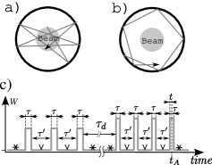
Figure 2: The trajectory of a single atom in a cell in the beam passing regime (a) and in the dark regime (b). (c) dependence of the optical pumping rate $W$ on time. The magnitude of $W$ depends on the velocity of the atom that causes the Doppler shift of the atom’s transition frequencies. The checkmarks show the times of elastic atom-wall collisions and the asterisks show the times of inelastic collisions.

Now let us consider more common case when some of the wall collisions change atomic velocity. After such a collision the atom being initially in the dark regime can either stay in this regime (which does not affect the equations for the density matrix) or switch to the beam passing regime. An atom that was being in the beam passing regime before the collision can either pass into the dark regime or get back to the beam passing regime, but with different value of the velocity and angle of reflection with the wall of the cell (and therefore with different values of $\tau$ and $\tau^{\prime}$). For sake of definiteness, let us call the time of entry of the atom into the beam zone after an inelastic collision as the beginning of the beam passing regime, and the time of exit from the beam zone as the end, respectively. Obviously, if the atom undergoes $N$ elastic collisions with the cell wall in the beam passing regime, then it goes $N$ times through the dark zone and $N+1$ times through the beam zone (see figure 2(c)).

The density matrix $\hat{\rho}_{e}$ describing the atom at the time of exit from the beam passing regime can be obtained similarly to the expression (13). It reads

$$\hat{\rho}_{e} = \biggl{[}\mathbb{I}+\rme^{\mathbb{A}\cdot\tau}\rme^{\mathbb{A}^{\prime}\cdot\tau^{\prime}}+\dots+\Bigl{(}\rme^{\mathbb{A}\cdot\tau}\rme^{\mathbb{A}^{\prime}\cdot\tau^{\prime}}\Bigr{)}^{N}\biggr{]}\Bigl{(}\mathbb{I}-\rme^{\mathbb{A}\cdot\tau}\Bigr{)}\hat{\rho}_{S}$$ (14)

$$+ \Bigl{(}\rme^{\mathbb{A}\cdot\tau}\rme^{\mathbb{A}^{\prime}\cdot\tau^{\prime}}\Bigr{)}^{N}\rme^{\mathbb{A}\cdot\tau}\hat{\rho}_{b}$$

$$= \Bigl{(}\mathbb{I}-\rme^{\mathbb{A}\cdot\tau}\rme^{\mathbb{A}^{\prime}\cdot\tau^{\prime}}\Bigr{)}^{-1}\biggl{[}\mathbb{I}-\Bigl{(}\rme^{\mathbb{A}\cdot\tau}\rme^{\mathbb{A}^{\prime}\cdot\tau^{\prime}}\Bigr{)}^{N+1}\biggr{]}\Bigl{(}\mathbb{I}-\rme^{\mathbb{A}\cdot\tau}\Bigr{)}\hat{\rho}_{S}$$

$$+ \Bigl{(}\rme^{\mathbb{A}\cdot\tau}\rme^{\mathbb{A}^{\prime}\cdot\tau^{\prime}}\Bigr{)}^{N}\rme^{\mathbb{A}\cdot\tau}\hat{\rho}_{b}\,.$$

Here, $\hat{\rho}_{b}$ is the density matrix of the atom at the time of beginning of the beam passing regime. It can be expressed via the density matrix $\hat{\rho}_{e,-1}$ for the previous time of exit from the beam passing regime (it is indicated by the index “$-1$”) using the expression (12)

$$\hat{\rho}_{b}=\rme^{\mathbb{A}^{\prime}\cdot\tau_{d}}\hat{\rho}_{e,-1}\,,$$ (15)

where $\tau_{d}$ is the time that atom spent in the dark. Similar to (14), one can obtain the expression for the density matrix at the observation time $t_{A}$:

$$\hat{\rho}(t_{A}) = \rme^{\mathbb{A}\cdot t}\rme^{\mathbb{A}^{\prime}\cdot\tau^{\prime}}\Bigl{(}\mathbb{I}-\rme^{\mathbb{A}\cdot\tau}\rme^{\mathbb{A}^{\prime}\cdot\tau^{\prime}}\Bigr{)}^{-1}\biggl{[}\mathbb{I}-\Bigl{(}\rme^{\mathbb{A}\cdot\tau}\rme^{\mathbb{A}^{\prime}\cdot\tau^{\prime}}\Bigr{)}^{n}\biggr{]}\Bigl{(}\mathbb{I}-\rme^{\mathbb{A}\cdot\tau}\Bigr{)}\hat{\rho}_{S}$$ (16)

$$+\Bigl{(}\mathbb{I}-\rme^{\mathbb{A}\cdot t}\Bigr{)}\hat{\rho}_{S}+\rme^{\mathbb{A}\cdot t}\Bigl{(}\rme^{\mathbb{A}^{\prime}\cdot\tau^{\prime}}\rme^{\mathbb{A}\cdot\tau}\Bigr{)}^{n}\hat{\rho}_{b}\,.$$

The expression for the excited state population $\rho_{33}$ reads

$$\rho_{33} = \hat{U}^{T}\biggl{\{}\rme^{\mathbb{A}\cdot t}\rme^{\mathbb{A}^{\prime}\cdot\tau^{\prime}}\Bigl{(}\mathbb{I}-\rme^{\mathbb{A}\cdot\tau}\rme^{\mathbb{A}^{\prime}\cdot\tau^{\prime}}\Bigr{)}^{-1}\biggl{[}\mathbb{I}-\Bigl{(}\rme^{\mathbb{A}\cdot\tau}\rme^{\mathbb{A}^{\prime}\cdot\tau^{\prime}}\Bigr{)}^{n}\biggr{]}\Bigl{(}\mathbb{I}-\rme^{\mathbb{A}\cdot\tau}\Bigr{)}\hat{\rho}_{S}$$ (17)

$$+\Bigl{(}\mathbb{I}-\rme^{\mathbb{A}\cdot t}\Bigr{)}\hat{\rho}_{S}+\rme^{\mathbb{A}\cdot t}\Bigl{(}\rme^{\mathbb{A}^{\prime}\cdot\tau^{\prime}}\rme^{\mathbb{A}\cdot\tau}\Bigr{)}^{n}\hat{\rho}_{b}\biggr{\}}+V\,.$$

Here, $n$ is the total number of collisions in the beam passing regime immediately prior to observation time $t_{A}$. Averaging the expressions (17), (14) and (15) over all the atoms in the beam zone, we obtain the average excited state population $\langle\rho_{33}\rangle$ that determines the absorption of light in the cell.

4 Ensemble averaging

4.1 General scheme of averaging

Let us consider in detail the averaging of (17). In this paper, we consider the excitation of the CPT-resonance by a laser whose spectral width is much smaller than the Doppler width of the optical transition. Hence, the main contribution to the resonance is given by the atoms with small longitudinal velocity, that are rarely colliding with the ends of the cell. We assume that the collisions of the atoms in the beam passing regime with the side walls of the cell do not change $v_{z}$. The average population $\langle\rho_{33}\rangle$ is

$$\langle\rho_{33}\rangle = \Bigl{\langle}\hat{U}^{T}\Bigl{(}\mathbb{I}-\rme^{\mathbb{A}\cdot t}\Bigr{)}\hat{\rho}_{S}\Bigr{\rangle}+\Bigl{\langle}\hat{U}^{T}\rme^{\mathbb{A}\cdot t}\Bigl{(}\rme^{\mathbb{A}^{\prime}\cdot\tau^{\prime}}\rme^{\mathbb{A}\cdot\tau}\Bigr{)}^{n}\Bigr{\rangle}\left\langle\hat{\rho}_{b}\right\rangle$$ (18)

$$+\langle V\rangle+\biggl{\langle}\hat{U}^{T}\rme^{\mathbb{A}\cdot t}\rme^{\mathbb{A}^{\prime}\cdot\tau^{\prime}}\Bigl{(}\mathbb{I}-\rme^{\mathbb{A}\cdot\tau}\rme^{\mathbb{A}^{\prime}\cdot\tau^{\prime}}\Bigr{)}^{-1}$$

$$\times\biggl{[}\mathbb{I}-\Bigl{(}\rme^{\mathbb{A}\cdot\tau}\rme^{\mathbb{A}^{\prime}\cdot\tau^{\prime}}\Bigr{)}^{n}\biggr{]}\Bigl{(}\mathbb{I}-\rme^{\mathbb{A}\cdot\tau}\Bigr{)}\hat{\rho}_{S}\biggr{\rangle},$$

where the angle brackets denote the averaging over the $z$-component of the velocity $v_{z}$, over the times $t$, $\tau$, $\tau^{\prime}$, $\tau_{d}$ and over the numbers $n$ and $N$ of elastic collisions in the beam passing regime prior the observation time $t_{A}$ and prior the exit from the beam passing regime (in the expression for $\langle\hat{\rho}_{b}\rangle$) respectively. The averaged density matrix $\langle\hat{\rho}_{b}\rangle$ of the atom entering the beam passing regime can be obtained by averaging of expressions (14) and (15):

$$\langle\hat{\rho}_{e}\rangle=\hat{C}+\mathbb{D}\langle\hat{\rho}_{b}\rangle,$$ (19)

$$\langle\hat{\rho}_{b}\rangle=\langle\rme^{\mathbb{A}^{\prime}\cdot\tau_{d}}\rangle\langle\hat{\rho}_{e}\rangle=\langle\rme^{\mathbb{A}^{\prime}\cdot\tau_{d}}\rangle\Bigl{(}\hat{C}+\mathbb{D}\langle\hat{\rho}_{b}\rangle\Bigr{)};$$ (20)

hence it is easy to find

$$\langle\hat{\rho}_{b}\rangle=\Bigl{(}\mathbb{I}-\langle\rme^{\mathbb{A}^{\prime}\cdot\tau_{d}}\rangle\mathbb{D}\Bigr{)}^{-1}\langle\rme^{\mathbb{A}^{\prime}\cdot\tau_{d}}\rangle\hat{C}.$$ (21)

Here

$$\hat{C}=\biggl{\langle}\Bigl{(}\mathbb{I}-\rme^{\mathbb{A}\cdot\tau}\rme^{\mathbb{A}^{\prime}\cdot\tau^{\prime}}\Bigr{)}^{-1}\biggl{[}\mathbb{I}-\Bigl{(}\rme^{\mathbb{A}\cdot\tau}\rme^{\mathbb{A}^{\prime}\cdot\tau^{\prime}}\Bigr{)}^{N+1}\biggr{]}\Bigl{(}\mathbb{I}-\rme^{\mathbb{A}\cdot\tau}\Bigr{)}\hat{\rho}_{S}\biggr{\rangle},$$ (22)

$$\mathbb{D}=\biggl{\langle}\Bigl{(}\rme^{\mathbb{A}\cdot\tau}\rme^{\mathbb{A}^{\prime}\cdot\tau^{\prime}}\Bigr{)}^{N}\rme^{\mathbb{A}\cdot\tau}\biggr{\rangle}\,.$$ (23)

Let us average over $n$ and $N$ first. Assuming that the probability of the elastic scattering $\alpha$ does not depend on the velocity of an atom and its internal state, we obtain the probability $P(n)=(1-\alpha)\alpha^{n}$ for $n$ consecutive elastic collisions. Hence, for any matrix $\mathbb{R}$ we get the matrix $\mathbb{R}^{n}$ averaged over $n$ as

$$\bigl{\langle}\mathbb{R}^{n}\bigr{\rangle}_{n}=\sum\limits_{n=0}^{\infty}P(n)\mathbb{R}^{n}=(1-\alpha)\bigl{(}\mathbb{I}-\alpha\mathbb{R}\bigr{)}^{-1}\,.$$ (24)

Exactly the same kind of distribution $P(N)=(1-\alpha)\alpha^{N}$ is valid for a total number of elastic collisions $N$ in the beam passing regime; therefore, the matrix $\mathbb{R}^{N}$ averaged over $N$ is described by the same expression: $\bigl{\langle}\mathbb{R}^{N}\bigr{\rangle}_{N}=\bigl{\langle}\mathbb{R}^{n}\bigr{\rangle}_{n}$.

The next steps are the averaging over times $t$, $\tau$, $\tau^{\prime}$ and $\tau_{d}$. It is obvious that the averaging over the time $\tau_{d}$ of atomic stay in the dark regime is independent on $t$, $\tau$, $\tau^{\prime}$, while $\tau$ and $\tau^{\prime}$, in general, are determined by transversal component of the atomic velocity in the beam passing regime and by the angle between the velocity and the wall of the cell. The time $t$ is determined also by atom’s position in the beam zone at the observation time $t_{A}$. Strictly speaking, one must integrate over four variables $t$, $\tau$, $\tau^{\prime}$ and $v_{z}$. However, we make a simplifying assumption which reduces the number of integration variables to 1.

In the beam passing regime atom goes $N$ times through the dark zone and $N+1$ times through the beam zone. Each passage through the dark zone takes time $\tau^{\prime}$ and each passage through the beam zone takes time $\tau$. Obviously, for each passage the times $\tau^{\prime}$ and $\tau$ are not independent. According to our assumption we consider times of different passages of the dark and light zones as independent random variables. We emphasize that this assumption refers only to ensemble averaging. In this case the averaged values of $\rme^{\mathbb{A}\cdot\tau}$, $\rme^{\mathbb{A}\cdot T}$, $\rme^{\mathbb{A}^{\prime}\cdot\tau^{\prime}}$ and $\rme^{\mathbb{A}^{\prime}\cdot\tau_{d}}$ in (18)–(23) can be calculated independently. Consider, for example, the averaged expression of $\rme^{\mathbb{A}\cdot\tau}$. Its easy to present this expression in the form [12]

$$\bigl{\langle}\rme^{\mathbb{A}\cdot\tau}\bigr{\rangle}_{\tau}=\mathbb{X}\left(\begin{array}[]{ccc}\bigl{\langle}\rme^{\lambda_{1}\tau}\bigr{\rangle}_{\tau}&0&0\\ 0&\bigl{\langle}\rme^{\lambda_{2}\tau}\bigr{\rangle}_{\tau}&0\\ 0&0&\bigl{\langle}\rme^{\lambda_{3}\tau}\bigr{\rangle}_{\tau}\end{array}\right)\mathbb{X}^{-1},$$ (25)

where $\mathbb{X}=(\hat{X}^{(1)},\hat{X}^{(2)},\hat{X}^{(3)})$ is the matrix constructed of the eigenvectors of $\mathbb{A}$ corresponding to the eigenvalues $\lambda_{1},\lambda_{2},\lambda_{3}$. Therefore, averaging over $\tau$ is reduced to the calculation of integrals

$$\langle\rme^{\lambda\tau}\rangle_{\tau}=g_{\tau}(\lambda)=\int_{0}^{\infty}\rme^{\lambda\tau}\cdot f_{\tau}(\tau)\,\rmd\tau\,,$$ (26)

that can be performed analytically. Here, $f_{\tau}$ is the probability density function of the random variable $\tau$. Averaging over $t$, $\tau^{\prime}$ and $\tau_{d}$ is analogous to (26) with functions $g_{\tau^{\prime}}(\lambda)$, $g_{t}(\lambda)$ and $g_{\tau_{d}}(\lambda)$. Note that $\mathop{\mathrm{Re}}(\lambda)<0$.

4.2 Averaging over $\tau$ and t

First of all, we find the probability density functions $f_{\tau}$ and $f_{t}$ of the random variables $\tau$ and $t$. The time $\tau$ that the atom spend in the beam zone is

$$\tau=\frac{2\sqrt{r^{2}-R^{2}\sin^{2}\varphi}}{v_{\perp}}\,,$$ (27)

where $\varphi$ is the angle between the atomic velocity projection on the plane orthogonal to the cell axis and the normal vector to the cell surface, $R$ is the radius of the cell, $r$ is the radius of the beam and $v_{\perp}$ is the component of the velocity orthogonal to $z$. Probability density function of the transversal velocity $v_{\perp}$ is the two-dimensional Maxwell distribution $M_{2}(v_{\perp})=2\exp(-v_{\perp}^{2}/v_{T}^{2})v_{\perp}/v_{T}^{2}$ where $v_{T}=\sqrt{2k_{B}T/m}$ is the most probable atomic velocity, $k_{B}$ is the Boltzmann constant, $T$ is the temperature, $m$ is the mass of the atom. The probability density $\Phi(\varphi)$ of the random variable $\varphi$ is proportional to $\cos\varphi$ [14, 34, 35]. Taking into account that in the beam passing regime the $\varphi$ takes values between $0$ and $\arcsin(r/R)$, we obtain $\Phi(\varphi)=R\cos\varphi/r$. Then, the cumulative distribution function $F_{\tau}(\tau)$ of the random variable  $\tau$ is

$$F_{\tau}(\tau) = \int\limits_{0}^{\arcsin(r/R)}\!\!\!\!\!\!\!\!\Phi(\varphi)\!\!\!\!\!\!\!\!\int\limits_{\frac{2\sqrt{r^{2}-R^{2}\sin^{2}\varphi}}{\tau}}^{\infty}\!\!\!\!\!\!\!\!{}M_{2}(v_{\perp})\,\rmd{}v_{\perp}\,\rmd\varphi$$ (28)

$$= \frac{\tau v_{T}\sqrt{\pi}}{4\rmi{}r}\,\rme^{-\frac{4r^{2}}{\tau^{2}v_{T}^{2}}}\,\mathrm{erf}\left(\frac{2\rmi{}r}{\tau v_{T}}\right)\,,$$

and the probability density function is

$$f_{\tau}(\tau)=\frac{\rmd{}F_{\tau}(\tau)}{\rmd\tau}=-\frac{1}{\tau}+\frac{v_{T}\sqrt{\pi}}{4\rmi{}r}\,\rme^{-\frac{4r^{2}}{\tau^{2}v_{T}^{2}}}\,\mathrm{erf}\left(\frac{2\rmi{}r}{\tau v_{T}}\right)\left[1+\frac{8r^{2}}{\tau^{2}v_{T}^{2}}\right]\,.$$ (29)

Note that the average time that the atom moves through the beam zone is

$$\bar{\tau}=\int_{0}^{\infty}f(\tau)\tau\,\rmd\tau=\int_{0}^{\infty}(1-F(\tau))\,\rmd\tau=\frac{\pi^{3/2}}{2}\frac{r}{v_{T}}\,.$$ (30)

Let us find the probability distribution function $f_{t}$ of time $t$ that atom stays continuously in the beam zone before the observation time $t_{A}$. The averaging is carried out over all the atoms in the beam zone. Let $\rmd{}n/\rmd{}t$ atoms arrive to the beam zone per unit of time. Then the total number of atoms in the beam zone is

$$N_{tot}=\frac{\rmd{}n}{\rmd{}t}\int_{0}^{\infty}(1-F_{\tau}(t^{\prime}))\,\rmd{}t^{\prime}.$$ (31)

Here, we took into account that $1-F_{\tau}(t^{\prime})$ is the atom’s probability to remain in the beam zone after time $t^{\prime}$ from the entrance to the beam. Therefore the number of atoms that have already spent time $t$ or more in the beam zone is

$$N_{t+}=\frac{\rmd{}n}{\rmd{}t}\int_{t}^{\infty}(1-F_{\tau}(t^{\prime}))\,\rmd{}t^{\prime}.$$ (32)

Hence, the cumulative distribution function $F_{t}(t)$ of the random variable $t$ reads

$$F_{t}(t)=1-\frac{\int_{t}^{\infty}\bigl{(}1-F_{\tau}(t^{\prime})\bigr{)}\,\rmd{}t^{\prime}}{\int_{0}^{\infty}\bigl{(}1-F_{\tau}(t^{\prime})\bigr{)}\,\rmd{}t^{\prime}}\,,$$ (33)

and the corresponding probability density function

$$f_{t}(t)=\frac{1-F_{\tau}(t)}{\int_{0}^{\infty}\bigl{(}1-F_{\tau}(t^{\prime})\bigr{)}\,\rmd{}t^{\prime}}=\frac{1-F_{\tau}(t)}{\bar{\tau}}\,,$$ (34)

is

$$f_{t}(t)=\frac{2v_{T}}{\pi^{3/2}r}\left[1-\frac{\tau v_{T}\sqrt{\pi}}{4\rmi{}r}\rme^{-\frac{4r^{2}}{\tau^{2}v_{T}^{2}}}\,\mathrm{erf}\left(\frac{2\rmi{}r}{\tau v_{T}}\right)\right]\,.$$ (35)

Using (34) it is easy to express $g_{\tau}(\lambda)$ in terms of $g_{t}(\lambda)$:

$$g_{\tau}(\lambda)=1+\lambda\,\bar{\tau}\,g_{t}(\lambda)$$ (36)

Note that the function $g_{t}(\lambda)=\int_{0}^{\infty}\rme^{\lambda x}\,f_{t}(t)\,\rmd{}t$ cannot be calculated in terms of elementary functions. We can find approximate but close to accurate result by replacing the precise expression (35) by some approximation similarly to [36]

$$f_{t}(t)\to\frac{v_{T}}{r}\tilde{f}_{t}\left(t\frac{v_{T}}{r}\right)\,,$$

$$\tilde{f}_{t}(x)=\frac{2}{\pi^{3/2}}\rme^{-bx}+\frac{16(1-\rme^{-ax})^{3}}{3\pi^{3/2}x^{2}}+Ax\rme^{-cx}\,.$$ (37)

We choose the values of coefficients $A=0.70839$, $a=0.49$, $b=2.286$ and $c=1.272$. These coefficients ensure (1) the same asymptotical behaviour of $f_{t}(t)$ and $\tilde{f}_{t}(tv_{T}/r)v_{T}/r$ at infinity, (2) coincidence of $f_{t}(t)$ and $\tilde{f}_{t}(tv_{T}/r)v_{T}/r$ near the zero to the second order with respect to $t$ and (3) correct normalization $\int_{0}^{\infty}\tilde{f}_{t}(x)\,\rmd{}x=1$. The plots of the functions $r\cdot f_{t}(x\cdot r/v_{T})/v_{T}$ and $\tilde{f}_{t}(x)$ are presented in figure 3.

Figure 3: Plots of $\tilde{f}_{t}\left(x\right)$ (dashed line) and $r{\cdot}f_{t}(x{\cdot}r/v_{T})/v_{T}$ (solid line)

The approximation (37) makes it possible to find the analytical expression for $g_{t}(\lambda)$:

$$g_{t}(\lambda)=\tilde{g}_{t}(\lambda r/v_{T})\,,$$

$$\tilde{g}_{t}(\Lambda) = \frac{2}{\pi^{3/2}}\frac{1}{b-\lambda}+\frac{A}{(c-\lambda)^{2}}$$ (38)

$$+\frac{16}{3\pi^{3/2}}\bigl{[}p(-\Lambda)-3p(a-\Lambda)+3p(2a-\Lambda)-p(3a-\Lambda)\bigr{]}\,,$$

where we denoted

$$p(\beta)=\beta\ln\beta\,.$$ (39)

It is easy to find $g_{\tau}(\lambda)$ from (38) and (36).

4.3 Averaging over $\tau^{\prime}$

Now let us calculate the function $g_{\tau^{\prime}}(\lambda)$. The time $\tau^{\prime}$ that the atom being in the beam passing regime spend in the dark zone continuously is

$$\tau^{\prime}=\frac{2}{v_{\perp}}\left(R\cos\varphi-\sqrt{r^{2}-R^{2}\sin^{2}\varphi}\;\right)\,.$$ (40)

If the beam diameter is much smaller than the cell diameter, the expression in brackets can be approximately replaces by the constant

$$\ell_{\perp} = 2\int_{0}^{\arcsin(r/R)}\left(R\cos\varphi-\sqrt{r^{2}-R^{2}\sin^{2}\varphi}\;\right)\Phi(\varphi)\,\rmd\varphi$$ (41)

$$= R\sqrt{1-\frac{r^{2}}{R^{2}}}-\frac{\pi r}{2}+\frac{R^{2}}{r}\arcsin\frac{r}{R}$$

that equals to average transversal path length in the dark zone. This approximation allows to readily obtain the cumulative distribution function $F^{\prime}$ of the random variable $\tau^{\prime}$:

$$F^{\prime}(\tau^{\prime})=\rme^{-\frac{\ell_{\perp}^{2}}{\tau^{\prime 2}v_{T}^{2}}}\,.$$ (42)

and

$$\overline{\tau}^{\prime}=\frac{\ell_{\perp}}{v_{T}}\sqrt{\pi}\,.$$ (43)

An attempt to directly calculate the function $g_{\tau^{\prime}}(\lambda)=\lambda\int_{0}^{\infty}(1-F^{\prime}(x))\rme^{\lambda x}\,\rmd{}x$ does not yield the result that can be expressed through elementary functions. As in previous case, we can find approximate but close to accurate result by replacing the precise expression (42) by

$$F^{\prime}(\tau^{\prime})\to\tilde{F}^{\prime}\left(\tau^{\prime}\frac{v_{T}}{\ell_{\perp}}\right)\,,$$

$$\tilde{F}^{\prime}(x)=\left\{\begin{array}[]{ll}1-\frac{\bigl{(}1-\rme^{-a(x-x_{0})}\bigr{)}^{4}}{(x-x_{0})^{2}}-\rme^{-b(x-x_{0})}\bigl{(}1+b(x-x_{0})\bigr{)}\,,&x>x_{0}\\ 0\,,&x\leq{}x_{0}\end{array}\right.$$ (44)

The values of the parameters $a=0.89$, $b=2.56$ and $x_{0}=0.3864$ ensure smoothness of the function $\tilde{F}^{\prime}(x)$ anywhere, good approximation of $F^{\prime}(x\ell_{\perp}/v_{T})$ in the region where it is appreciably different from zero (see figure 4) and get the correct value of time $\bar{\tau}^{\prime}$.

Figure 4: Plots of functions $\tilde{F}^{\prime}(x)$ (dashed line) and $F^{\prime}({x\ell_{\perp}/v_{T}})$ (solid line).

Using the approximation function (44), we find

$$g_{\tau^{\prime}}(\lambda)\approx\tilde{g}^{\prime}(\lambda\ell_{\perp}/v_{T})\,,$$

$$\tilde{g}^{\prime}(\Lambda) = \Lambda\rme^{\Lambda x_{0}}\left[\frac{2b-\Lambda}{(b-\Lambda)^{2}}+p(4a-\Lambda)-4p(3a-\Lambda)\right.$$ (45)

$$\left.-4p(a-\Lambda)+6p(2a-\Lambda)+p(-\Lambda)+\frac{1}{\Lambda}\right]\,.$$

4.4 Averaging over $\tau_{d}$

The last function we should find for calculating the fluorescence of the atoms in the cell is $g_{\tau_{d}}(\lambda)$. The exact calculation of the probability density function $f_{d}$ of the random variable $\tau_{d}$ is a nontrivial problem, because in the dark regime the trajectory of the atom consists of a random number of segments of random length; along each of them the atom moves with a random velocity. Nevertheless, it is clear that the probability density exponentially tends to zero when $\tau_{d}\to 0$. The minimal distance that an atom can pass in dark regime in the transverse direction is $2(R-r)$. The transverse velocity $v_{\perp}$ of the atom with the probability greater than 98% is less than $2v_{T}$, so we assume that $f_{d}(\tau_{d})=0$ when $\tau_{d}<\tau_{0}=(R-r)/v_{T}$. If the beam diameter is much smaller than the diameter of the cell, the atom usually returns from the dark regime into the beam passing regime after many wall collisions. The probability for atom to return to the beam passing regime after certain collision does not depend on the number of previous collisions. Such processes are usually described by an exponential probability distribution function, so for the function $f_{d}(\tau_{d})$ of the random variable $\tau_{d}$ we take

$$f_{d}(\tau_{d})=\left\{\begin{array}[]{ll}h\rme^{-h(\tau_{d}-\tau_{0})}\,,&\tau_{d}>\tau_{0}\\ 0\,,&\tau_{d}<\tau_{0}\,,\end{array}\right.$$ (46)

where $h=1/(\bar{\tau}_{d}-\tau_{0})$, $\bar{\tau}_{d}$ is the average time of atom’s being in the dark zone. From (26) and (46) it is easy to get $g_{\tau_{d}}(\lambda)=\rme^{\lambda\tau_{0}}/(1-\lambda/h)$.

The value of $\bar{\tau}_{d}$ can be found from the “time balance” conditions. It means that the total time that an atom spends in the beam or in the dark zone is proportional to the volume of this zone. Consider the cycle in which an atom being in the beam passing regime undergoes $N$ elastic collisions with the wall, and then moves into the dark regime. The history of any atom can be represented as a sequence of such cycles. The total time $t_{b}$ spent by an atom in the beam zone over the cycle is $t_{b}=(N+1)\tau$. In turn, the time $t_{d}$ spent by the atom in a dark zone during the cycle is $t_{d}=\tau_{d}+N\tau^{\prime}$. The ratio of averaged times $t_{b}$ and $t_{d}$ over the different cycles must be equal to the ratio of volumes of the bright and dark zones. Hence, we find

$$\bar{\tau}_{d}=\left(\frac{R^{2}}{r^{2}}-1\right)\bar{\tau}(\bar{N}+1)-\bar{\tau}^{\prime}\bar{N},$$ (47)

where $\bar{N}=\alpha/(1-\alpha)$ is the average number of successive elastic collisions with the cell wall.

In the conclusion of this section we write down the expression for the averaged excited state population:

$$\langle\rho_{33}\rangle=\int\limits_{-\infty}^{\infty}M_{1}(v_{z})\,\hat{U}^{T}\mathbb{G}_{t}(1-\alpha)\bigg{(}\mathbb{I}-\alpha\,\mathbb{G}^{\prime}_{\tau^{\prime}}\mathbb{G}^{\prime}_{\tau^{\prime}}\bigg{)}^{-1}dv_{z}\cdot\ \langle\hat{\rho}_{b}\rangle$$

$$+\int\limits_{-\infty}^{\infty}M_{1}(v_{z})Vdv_{z}+\int\limits_{-\infty}^{\infty}M_{1}(v_{z})\,\hat{U}^{T}\Bigg{[}\left(\mathbb{I}-\mathbb{G}_{t}\right)+\mathbb{G}_{t}\mathbb{G}^{\prime}_{\tau^{\prime}}$$

$$\times\left(\mathbb{I}-\mathbb{G}_{\tau}\mathbb{G}^{\prime}_{\tau^{\prime}}\right)^{-1}\Big{[}\mathbb{I}-(1-\alpha)\bigg{(}\mathbb{I}-\alpha\mathbb{G}_{\tau}\mathbb{G}^{\prime}_{\tau^{\prime}}\bigg{)}^{-1}\Big{]}\Bigg{]}\hat{\rho}_{s}\,dv_{z},$$

where $M_{1}(v_{z})=\rme^{-v_{z}/v_{T}}/(v_{T}\sqrt{\pi})$ is one-dimensional Maxwell distribution function,

$$\mathbb{G}_{t} = \mathbb{X}\left(\begin{array}[]{ccc}g_{t}(\lambda_{1})&0&0\\ 0&g_{t}(\lambda_{2})&0\\ 0&0&g_{t}(\lambda_{3})\end{array}\right)\mathbb{X}^{-1},$$ (52)

$$\mathbb{G}_{\tau} = \mathbb{X}\left(\begin{array}[]{ccc}g_{\tau}(\lambda_{1})&0&0\\ 0&g_{\tau}(\lambda_{2})&0\\ 0&0&g_{\tau}(\lambda_{3})\end{array}\right)\mathbb{X}^{-1},$$ (56)

$$\mathbb{G}^{\prime}_{\tau^{\prime}} = \mathbb{X}^{\prime}\left(\begin{array}[]{ccc}g_{\tau^{\prime}}(\lambda^{\prime}_{1})&0&0\\ 0&g_{\tau^{\prime}}(\lambda^{\prime}_{2})&0\\ 0&0&g_{\tau^{\prime}}(\lambda^{\prime}_{3})\end{array}\right)\mathbb{X}^{\prime-1}$$ (60)

$$\langle\hat{\rho}_{b}\rangle = \bigg{(}\mathbb{I}-\langle\mathbb{G}^{\prime}_{\tau_{d}}\rangle\mathbb{D}\bigg{)}^{-1}\langle\mathbb{G}^{\prime}_{\tau_{d}}\rangle\hat{C},$$ (61)

where expressions (22,23) for $\hat{C}$ and $\mathbb{D}$ can be rewritten as

$$\hat{C} = \int\limits_{-\infty}^{\infty}M_{1}(v_{z})\Big{(}\mathbb{I}-\mathbb{G}_{\tau}\mathbb{G}^{\prime}_{\tau^{\prime}}\Big{)}^{-1}\Big{[}\mathbb{I}-(1-\alpha)\mathbb{G}_{\tau}\mathbb{G}^{\prime}_{\tau^{\prime}}$$ (62)

$$\times\Big{(}\mathbb{I}-\alpha\mathbb{G}_{\tau}\mathbb{G}^{\prime}_{\tau^{\prime}}\Big{)}^{-1}\Big{]}\big{(}\mathbb{I}-\mathbb{G}_{\tau}\big{)}\hat{\rho}_{s}\;dv_{z},$$

$$\mathbb{D} = \int\limits_{-\infty}^{\infty}M_{1}(v_{z})\;\mathbb{G}_{\tau}(1-\alpha)\Big{(}\mathbb{I}-\alpha\mathbb{G}^{\prime}_{\tau^{\prime}}\mathbb{G}_{\tau}\Big{)}^{-1}\,dv_{z},$$ (63)

$$\langle\mathbb{G}^{\prime}_{\tau_{d}}\rangle = \int\limits_{-\infty}^{\infty}M_{1}(v_{z})\mathbb{X}^{\prime}\left(\begin{array}[]{ccc}g_{\tau_{d}}(\lambda^{\prime}_{1})&0&0\\ 0&g_{\tau_{d}}(\lambda^{\prime}_{2})&0\\ 0&0&g_{\tau_{d}}(\lambda^{\prime}_{3})\end{array}\right)\mathbb{X}^{\prime-1}\,dv_{z}.$$ (67)

5 Results of calculations.

An absorption of the laser power in the cell filled by the gas of three-level $\Lambda$-atoms is proportional to the average excited state population described by expression (18). Typical parameters of ⁸⁷Rb atom in vacuum cell were taken as the parameters of the $\Lambda$-atom in our calculations. The atomic mass $m$ was assumed to be equal to the mass of ${}^{87}\mathrm{Rb}$ isotope, the temperature $T=20^{\circ}\mathrm{C}$, the ground state relaxation rate $\Gamma=300\,\mathrm{s}^{-1}$, the optical coherence relaxation rate $\gamma^{\prime}=1.8\times 10^{7}\,\mathrm{s}^{-1}$. We assume $V_{1}=V_{2}=V$ and we set the optical detuning $\Omega_{L}=0$. Calculations were performed for the cell radius $R=0.5$ cm and for three values of the laser beam radius $r$ ($r=0.5$, $1.5$ and $5\,\mbox{mm}$) and for five values of the probability $\alpha$ of the atomic-wall elastic collision ($\alpha=0$, $0.25$, $0.5$, $0.75$ and $1$).

The structure of the CPT resonance for $\alpha=0$ was discussed in [11, 12, 13, 14]. Resonance consists of a broad pedestal whose width is about several tens of kilohertz and of a narrow central peak (see figure 5(a)).

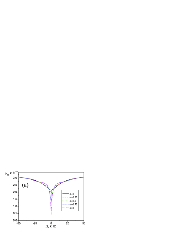
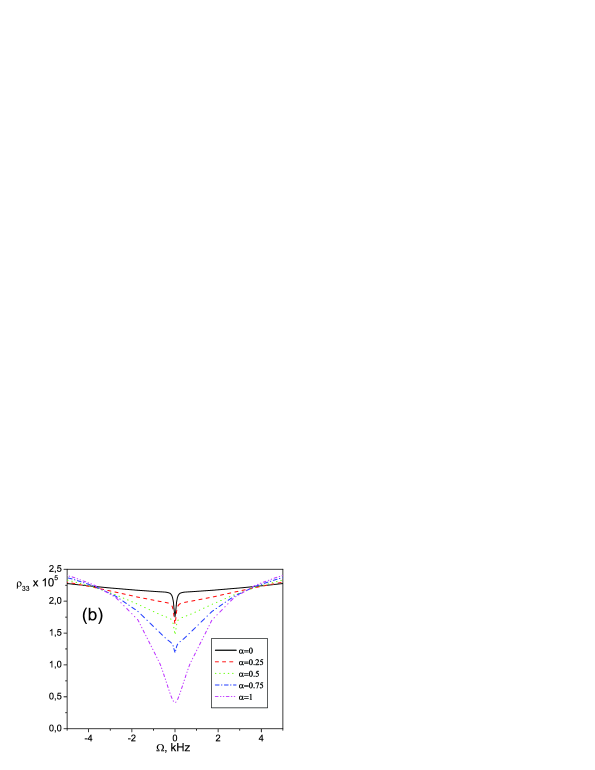
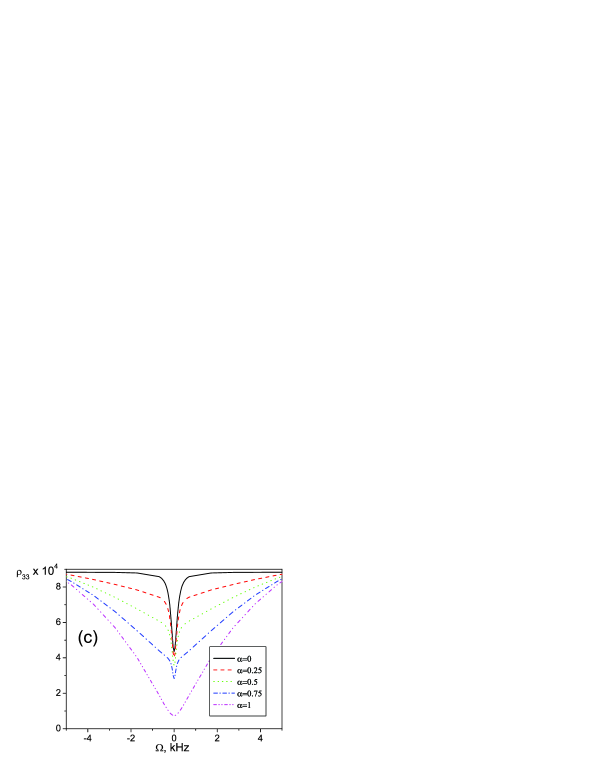
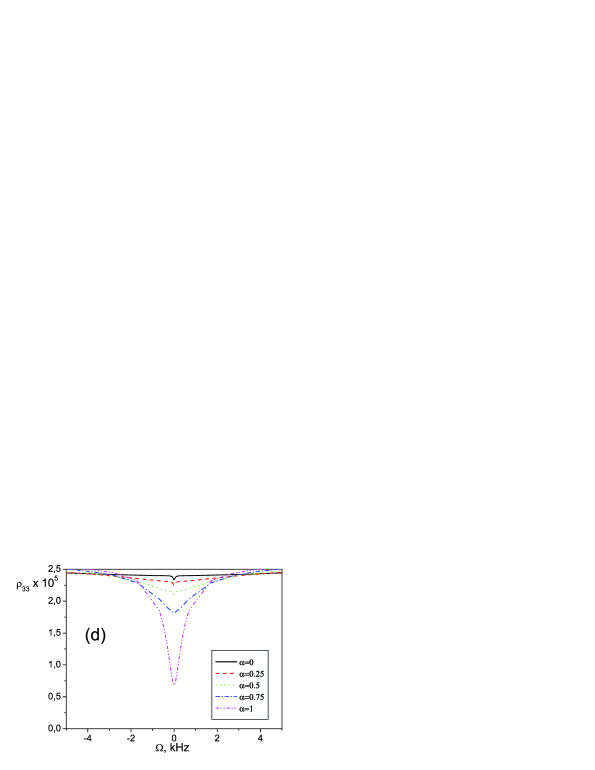
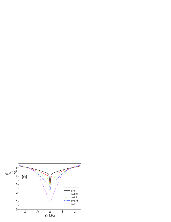
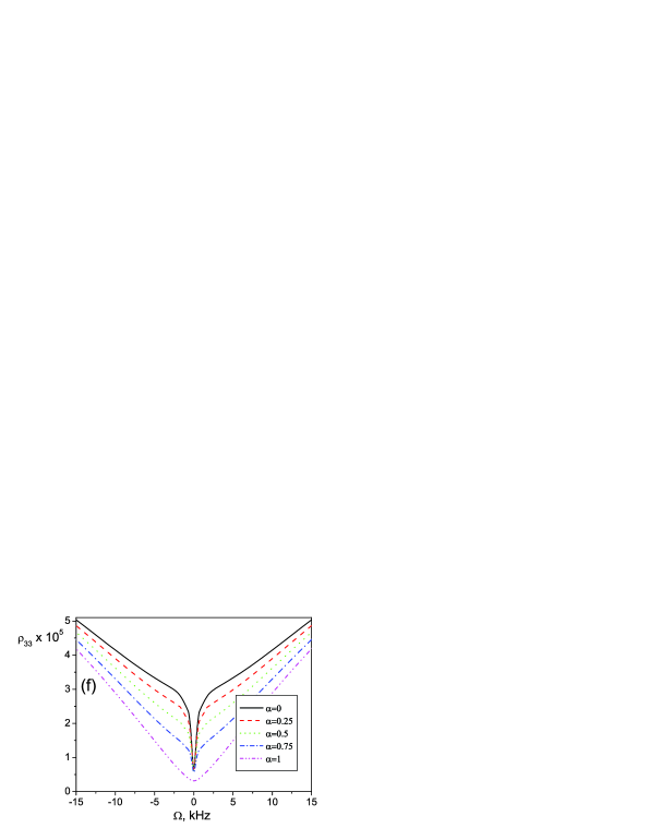
Figure 5: The shape of CPT resonance for different $\alpha$, $V$ and $r$. Parameters: $r=1.5\,\mbox{mm}$, $V=7.7\times 10^{5}\,\mbox{s}^{-1}$ (a, b); $r=0.5\,\mbox{mm}$, $V=1.46\times 10^{7}\,\mbox{s}^{-1}$ (c); $r=0.5\,\mbox{mm}$, $V=7.3\times 10^{5}\,\mbox{s}^{-1}$ (d); $r=5\,\mbox{mm}$, $V=3.3\times 10^{5}\,\mbox{s}^{-1}$ (e); $r=5\,\mbox{mm}$, $V=1.46\times 10^{6}\,\mbox{s}^{-1}$ (f);

Broad background is formed by the atoms that have passed through the beam zone only once, whereas the central peak is formed by multiple passes. If the elastic collision probability $\alpha$ is nonzero, the additional “intermediate” structure in CPT resonance appears. This is a peak whose width is greater than the width of the narrow central peak, but less than the width of the broad background. This peak is formed by atoms that pass the beam zone many times in beam passing regime. It should be noted that in the elastic collision act the atomic longitudinal velocity $v_{z}$ remains constant, in contrast with the case of inelastic scattering when atoms pass the beam zone just once in the beam passing regime. This fact explains the occurrence of “intermediate” structure depending on $\alpha$ when the cell radius coincides with the radius of the beam (see figure 5(e) and (f)). Indeed, in the considered case of the laser field with narrow spectral linewidth only the atoms with small $|v_{z}|$ contribute to the CPT resonance. The “intermediate” structure is formed by the atoms that remains in this velocity group during several passage through the cell volume whereas the narrow structure is formed by the atoms that change their velocities after one wall collision.

At Fig. 5(a)–(f) we see that the higher elastic collision probability $\alpha$ corresponds to a lower excited state population at $\Omega=0$. To explain it we should note that for higher $\alpha$ atoms spent longer time in the beam passing regime; therefore, they have more time to came into the dark state.

It should be noted that if $\alpha=1$, the narrow peak disappears. It can be explained by the fact that all the atoms contributing to the CPT resonance formation are in the beam passing regime permanently. These atoms spent relative higher part of time in the beam zone than all the atoms in case of $\alpha=0$. Therefore, the narrow peak is formed by atoms which passed the beam, then spend quite a long time in the dark regime and then returned back to the beam. Intermediate structure is formed by atoms which passed the beam several times repeatedly in the beam passing regime. The time between two subsequent beam passage occurs to be smaller than in the case of inelastic collision. Therefore, the resonance occurs to be broader. The broad pedestal is formed by atoms that pass the beam zone once during the coherence time.

6 Conclusions

We developed a theory of the coherent population trapping resonance in a cylindrical cell filled with antirelaxation coated walls. The laser beam is assumed to have constant intensity in cylindrical region. The atom-wall interaction is described by the probability of elastic collisions. It is shown that the nonzero probability of elastic collision leads to distortion of the CPT resonance lines that consists in appearance of the additional peak formed by the atoms, repeatedly passing through the beam zone in the beam passing regime. The general scheme of calculation can be applied not only to CPT formation in wall-coated cells but also for the cell with small buffer gas pressure (much lower than the necessary for the diffusion approximation applicability). Another possible application can be connected with the high-precision clock based on an ensemble of cold atoms or ions, e.g. ions of ${}^{229}\mbox{Th}$ [37]. The energy splitting of the ${}^{229}\mbox{Th}$ ground-state doublet is about $7.6\mbox{eV}$ [38] corresponding to vacuum ultraviolet and long, about an hour, expected half-life of the excited state of the nuclei [39] makes this nuclei a possible promising object for nuclear frequency standard. The study of one-photon resonances in the two-dimensional trap with zonal pumping may be applicable to the spectroscopy of this nucleus.

References

References

• [1] Alzetta G, Gozzini A, Moi L and Orriols G 1976 Nuovo Cimento B 36 5–20
• [2] Arimondo E and Orriols G 1976 Lett. Nuovo Cimento 17 333–8
• [3] Gray H R, Whitley R W and Stroud C R Jr 1978 Opt. Lett. 3 218–20
• [4] Harris S E 1997 Phys. Today 50 36–42
• [5] Knappe S, Wynands R, Kitching J, Robinson H G and Hollberg L 2001 J. Opt. Soc. Am. B 18, 1545–53
• [6] Vanier J 2005 Applied Physics B 81 421–2.
• [7] Bergmann K, Theur H and Shore B W 1998 Rev. Mod. Phys. 70 1003–25
• [8] Aspect A, Arimondo E, Kaiser R, Vansteenkiste N and Cohen-Tannoudji C 1988 Phys. Rev. Lett. 61 826–9
• [9] Nagel A, Graf L, Naumov A, Mariotti E, Biancalana V, Meschede D and Wynands R 1998 Europhys. Lett. 44 31–6
• [10] Schwindt P D D, Knappe S, Shah V, Hollberg L, Kitching J, Liew L-A and Moreland J 2004 Appl. Phys. Lett. 85 6409–11
• [11] Breschi E, Kazakov G, Schori C, Domenico G Di, Mileti G, Litvinov A and. Matisov B 2010 Phys. Rev. A 82 063810
• [12] Kazakov G A, Matisov B G and Litvinov A N 2010 Nauchno-Technicheskie Vedomosti SPbGPU 4 11–20 (in Russian)
• [13] Klein M, Hohensee M, Phillips D F and Walsworth R L 2011 Physical Review A 83 013826
• [14] Hohensee M 2009 Testing Fundamental Lorentz Symmetries of Light, Ph.D. thesis (Harvard University)
• [15] Ye C Y and Zibrov A S 2002 Phys. Rev. A. 65. 023806
• [16] Klein M, Novikova I, Phillips D F and Walsworth R L 2006 Journ. Mod. Opt. 53 2583–91
• [17] Xiao Y 2009 Mod. Phys. Lett. B 23 661–80
• [18] Xiao Y, Novikova I, Phillips D F and Walsworth R L 2008 Opt. Express 16 14128–41
• [19] Romanenko V I, Romanenko A V and Yatsenko L P 2010 Ukr. J. Phys. 55 393–402
• [20] Vanier J, Audoin C 1989 The quantum physics of Atomic Frequency Standards (Bristol: Adam Higler) 1567 pp
• [21] Bouchiat M A and Brossel J 1966 Phys. Rev. 147 41–54.
• [22] Balykin V I, Letokhov V S, Ovchinnikov Yu B and Sidorov A I 1988 Phys. Rev. Lett. 60 2137–40
• [23] Kasevich M A, Weiss D S and Chu S 1990 Opt. Lett. 15 607–9
• [24] Vladimirskii V V 1961 Sov. Phys. — JETP 12 740–6
• [25] Opat G I, Wark S and Cimmino A 1992 Appl. Phys. B. 54 396–402
• [26] Hayward T J at al 2010 J. Appl. Phys. 108, 043906
• [27] Mazets I E and Matisov B G 1992 Sov. Phys. — JETP 74 13–7
• [28] Stenholm S 2005 Foundations of laser spectroscopy (New York: Dover) 268 pp.
• [29] Shore B W 1990 The Theory of Coherent Atomic Excitation, Vol. 1 (New York: Wiley) 774 pp.
• [30] Dicke R H 1953 Phys. Rev. 89 472–3
• [31] Kazakov G, Matisov B, Litvinov A and Mazets I 2007 J. Phys. B: At. Mol. Opt. Phys. 40 3851–60
• [32] Litvinov A N, Kazakov G A, Matisov B G 2009 J. Phys. B: At. Mol. Opt. Phys. 42 165402
• [33] Jaynes E T 1955 Phys. Rev. 98 1099–105
• [34] Frueholz R P and Volk C H 1985 J. Phys. B: At. Mol. Phys. 18 4055–67
• [35] Bhaskar N D, Kahla C M and Martin L R 1990 Carbon 28 71–8.
• [36] Mazets I E and Shifrin L B 2000 Opt. Commun. 175 227–31
• [37] Peik E and Tamm Chr 2003 Europhys. Lett. 61 181–6.
• [38] Beck B R, Becker J A, Beiersdorfer P, Brown G V Moody K J, Wilhelmy J B, Porter F S, Kilbourne C A and Kelly R L 2007 Phys. Rev. Lett. 98 142501.
• [39] Tkalya E V, Zherykhin A N and Zhudov V I 2000 Phys. Rev. C 61 064380.