Singular Casimir Elements of the Euler Equation and Equilibrium Points

Abstract.

The problem of the nonequivalence of the sets of equilibrium points and energy-Casimir extremal points, which occurs in the noncanonical Hamiltonian formulation of equations describing ideal fluid and plasma dynamics, is addressed in the context of the Euler equation for an incompressible inviscid fluid. The problem is traced to a Casimir deficit, where Casimir elements constitute the center of the Poisson algebra underlying the Hamiltonian formulation, and this leads to a study of singularities of the Poisson operator defining the Poisson bracket. The kernel of the Poisson operator, for this typical example of an infinite-dimensional Hamiltonian system for media in terms of Eulerian variables, is analyzed. For two-dimensional flows, a rigorously solvable system is formulated. The nonlinearity of the Euler equation makes the Poisson operator inhomogeneous on phase space (the function space of the state variable), and it is seen that this creates a singularity where the nullity of the Poisson operator (the “dimension” of the center) changes. The problem is an infinite-dimension generalization of the theory of singular differential equations. Singular Casimir elements stemming from this singularity are unearthed using a generalization of the functional derivative that occurs in the Poisson bracket.

1. Introduction

Equations that describe ideal fluid and plasma dynamics in terms of Eulerian variables are Hamiltonian in terms of noncanonical Poisson brackets, degenerate brackets in noncanonical coordinates. Because of degeneracy, such Poisson brackets possess Casimir elements, invariants that have been used to construct variational principles for equilibria and stability. However, early on it was recognized that typically there are not enough Casimir elements to obtain all equilibria as extremal points of these variational principles. In [26, 28] it was noted that this Casimir deficit is attributable to rank changing of the operator that defines the noncanonical Poisson bracket. Thus, a mathematical study of the kernel of this operator is indicated, and this is the main purpose of the present article.

Recognizing a Hamiltonian flow as a differential operator, the point where the rank of the Poisson bracket changes is a singularity, from which singular (or intrinsic) solutions stem. When we consider a Hamiltonian flow on a function space, the problem is an infinite-dimension generalization of the theory of singular differential equations; the derivatives are functional derivatives, and the construction of singular Casimir elements amounts to integration in an infinite-dimension space. In order to facilitate this study, it is necessary to place the noncanonical Hamiltonian formalism on a more rigorous footing, and this subsidiary purpose is addressed in the context of Euler’s equation of fluid mechanics, although the ideas presented are of more general applicability than this particular example.

We start by reviewing finite-dimensional canonical and noncanonical Hamiltonian mechanics, in order to formulate our problem. These dynamical system have the form

$$\frac{d{z}}{dt}=J\,\partial_{{z}}H({z})\,,$$ (1.1)

where ${z}=(z^{1},z^{2},\dots,z^{m})$ denotes a set of phase space coordinates, $H$ is the Hamiltonian function with $\partial_{z}$ its gradient, and the $m\times m$ matrix $J$ (variously called e.g. the cosymplectic form, Poisson tensor, or symplectic operator) is the essence of the Poisson bracket and determines important Lie algebraic properties [26] (see also Remark 1.1).

For canonical Hamiltonian systems of dimension $m=2n$ the matrix $J$ has the form

$$J_{c}=\left(\begin{array}[]{cc}~{}~{}0_{n}\hfill&I_{n}\\ -I_{n}&0_{n}\hfill\\ \end{array}\right)\,.$$ (1.2)

Noncanonical Hamiltonian systems allow a $z$-dependent $J({z})$ (assumed here to be a holomorphic function) to have a kernel, i.e.  $\mathrm{Rank}(J({z}))$ may be less than $m$ and may change as a function of ${z}$.

From (1.1) it is evident that equilibrium points of the dynamics, i.e. points for which $d{z}/dt=0\ \forall t$, satisfy

$$\partial_{{z}}H({z})=0\,.$$ (1.3)

However, in the noncanonical case these may not be the only equilibrium points of a given Hamiltonian $H({z})$, because degeneracy gives rise to Casimir elements $C({z})$, nontrivial (nonconstant) solutions to the differential equation

$$J({z})\partial_{{z}}C({z})=0\,.$$ (1.4)

Given such a $C({z})$, replacement of the Hamiltonian by $H({z})+C({z})$ does not change the dynamics. Thus, an extremal point of

$$\partial_{{z}}[H({z})+C({z})]=0$$ (1.5)

will also give an equilibrium point. Note, in light of the homogeneity of (1.4) an arbitrary multiplicative constant can be absorbed into $C$ and so (1.5) can give rise to families of equilibrium points.

If $\mathrm{Rank}(J({z}))=m=2n$, (1.4) has only the trivial solution $C({z})=$ constant. If $\mathrm{Rank}(J({z}))=2n<m$ and $n$ is constant, then (1.4) has $m-2n$ functionally independent solutions (Lie-Darboux theorem). The problem becomes more interesting if there is a singularity where $\mathrm{Rank}(J({z}))$ changes: in this case we have a singular (hyperfunction) Casimir element (see Fig. 1). For example, consider the one-dimensional system where $J=ix$ ($x\in\mathbb{R}$). At $x=0$ $\mathrm{Rank}(J)$ drops to 0, and this point is a singular point of the differential equation $J(x)\partial_{x}C=0$. The singular Casimir element is $C(x)={Y}(x)$, where $Y$ is the Heaviside step function.

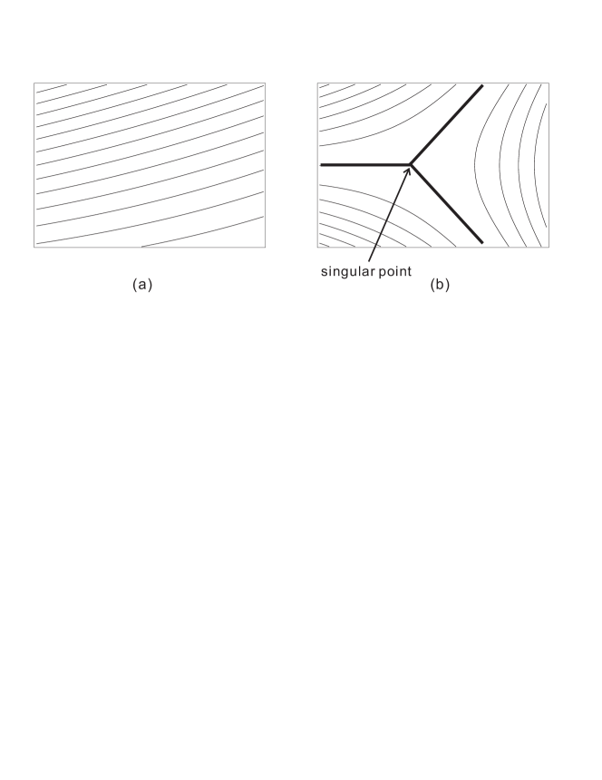
Figure 1. Low-dimensional cartoon of a foliated phase space. (a) Depiction of level-sets (leaves) of Casimir elements foliating the phase space. Since a Casimir element is a constant of motion, every orbit is constrained to a leaf determined by a Casimir element. In this cartoon of a two-dimensional phase space, each Casimir (symplectic) leaf has codimension one, hence in this depiction the effective space of dynamics has dimension one. (b) Depiction of phase space with a singular point where $\mathrm{Rank}(J)$ changes. The codimension of the Casimir foliation changes, resulting in a singular Casimir leaf (with the determining Casimir element being a hyperfunction). In the figure the codimension of the Casimir leaf at the singular point is two, hence the singular point is an equilibrium point. In higher-dimensional (infinite-dimensional) phase space, a singular point may have far richer structure. In Sec. 3, we delineate how a singular point is created in an infinite-dimensional phase space by examining an infinite-dimensional Hamiltonian system of Eulerian fluid (to be formulated in Sec. 2). In Sec. 4, we will study the structure of the singular point (which is still infinite-dimensional) by examining equilibrium points.

We generalize (1.1) further to include infinite-dimension systems. Let $u\in X$ be the state variable, where for now $X$ is some unspecified function space, $\mathcal{J}(u)$ be a linear antisymmetric operator in $X$ that generally depends on $u$ (for a fixed $u$, $\mathcal{J}(u)$ may be regarded as a linear operator $X\rightarrow X$ – see Remark 1.2 below), and $H(u)$ be a functional $X\rightarrow\mathbb{R}$. Introducing an appropriate functional derivative (gradient) $\partial_{u}H(u)$, we consider evolution equations of the form

$$\partial_{t}u=\mathcal{J}(u)\partial_{u}H(u)\,,$$ (1.6)

where $\partial_{t}u:=\partial u/\partial t$. A Casimir element $C(u)$ (a functional $X\rightarrow\mathbb{R}$) is a nontrivial solution to

$$\mathcal{J}(u)\partial_{u}C(u)=0\,.$$ (1.7)

We may solve (1.7) by two steps:

1. Find the kernel of $\mathcal{J}(u)$, i.e., solve a “linear equation” (cf. Remark 1.2)

   $$\mathcal{J}(u)v=0$$ (1.8)

   to determine $v$ for a given $u$, which we write as $v(u)$.

2. “Integrate” $v(u)$ with respect to $u$ to find a functional $C(u)$ such that $v(u)=\partial_{u}C(u)$.

As evident in the above finite-dimension example, step-1 should involve “singular solutions” if $\mathcal{J}(u)$ has singularities. Then, step-2 will be rather nontrivial – for singular Casimir elements, we will need to generalize the notion of functional derivative. As mentioned above, the present paper is devoted to such an extension of the notion of Casimir elements in infinite-dimensional noncanonical Hamiltonian systems. Specifically, we invoke the Euler equation of ideal fluid mechanics as an example, but much carries over to other systems since many fluid and plasma systems share the same operator $\mathcal{J}$. In Sec. 2, we will describe the Hamiltonian form of Euler’s equation, which places on a more rigorous footing the formal calculations of [20, 21, 22, 23, 24, 32]. In Sec. 3.1, we will analyze the kernel of the corresponding Poisson operator $\mathcal{J}(u)$ and its singularity. A singular Casimir element and its appropriate generalized functional derivative (gradient) will be given in Sec. 3.2.

The relation between the (generalized) Casimir elements and equilibrium points (stationary ideal flows) will be discussed in Sec. 4. Generalizing (1.5) to an infinite-dimensional space, we may find an extended set of equilibrium points by solving

$$\partial_{u}[H(u)+C(u)]=0.$$ (1.9)

We note, however, it is still uncertain whether or not every equilibrium point can be obtained from Casimir elements in this way. For example, let us consider a simple Hamiltonian $H(u)=\|u\|^{2}/2$ (in Appendix A, the Hamiltonian of the Euler equation is given in terms of the velocity field $\bm{u}$, which here corresponds to the state variable $u$). Then, $\partial_{u}H(u)=u$ and (1.6) reads

$$\partial_{t}u=\mathcal{J}(u)u.$$ (1.10)

The totality of nontrivial equilibrium points is $\mathrm{Ker}(\mathcal{J}(u))$. For $v\in\mathrm{Ker}(\mathcal{J}(u))$ to be characterized by (1.9), which now simplifies to $u=-\partial_{u}C(u)$, we encounter the “integration problem,” i.e., we have to construct $C(u)$ such that $v(u)=\partial_{u}C(u)$ for every $v(u)\in\mathrm{Ker}(\mathcal{J}(u))$ – this may not be always possible. On the other hand, even for a given $C(u)$, the “nonlinear equation” $u=-\partial_{u}C(u)$ does not necessarily have a solution – in Sec. 4.2 we will show some examples of no-solution equations. While we leave this question (the “integrability” of all equilibrium points) open, the present effort shows it is sometimes possible and provides a more complete understanding of the stationary states of infinite-dimensional dynamical systems. In Sec. 5 we give some concluding remarks.

Remark 1.1.

We endow the phase space $X$ of state variable $u$ (${z}$ if $X$ is finite-dimensional) with an inner product $(a,b)$. Let $F:\,X\rightarrow\mathbb{R}$ be an arbitrary smooth functional (function if $X$ is finite-dimensional). If $u$ obeys (1.6) in a Hilbert space (or (1.1) for finite-dimensional systems), the evolution of $F(u)$ obeys $dF({u})/dt=[F({u}),H({u})]$, where

$$[F({u}),H({u})]=(\partial_{{u}}F({u}),\mathcal{J}({{u}})\partial_{{u}}H({u}))$$

is an antisymmetric bilinear form. If this bracket $[~{},~{}]$ satisfies the Jacob identity, it defines a Poisson algebra, a Lie algebra realization on functionals. A Casimir element $C$ is a member of the center of the Poisson algebra, i.e., $[C,G]=0$ for all $G$. The bracket defined by the Poisson operator of Sec. 2.4 satisfies the Jacobi’s identity [22, 24, 26]. The Jacobi identity is satisfied for all Lie-Poisson brackets, a class of Poisson brackets that describe matter that are built from the structure constants of Lie algebras (see, e.g., [26]). For finite-dimensional systems there is a beautiful geometric interpretation of such brackets where phase space is the dual of the Lie algebra and surfaces of constant Casimirs, coadjoint orbits, are symplectic manifolds. Unfortunately, in infinite-dimensions, i.e., for nonlinear partial differential equations, there are functional analysis challenges that limit this interpretation (see, e.g., [15]). (For example, for the incompressible Euler fluid equations the group is that of volume preserving diffeomorphisms.) In terms of this interpretation, the analysis of the present paper can be viewed as a local probing of the coadjoint orbit.

Remark 1.2.

In (1.6), the operator $\mathcal{J}(u)$ must be evaluated at the common $u$ of $\partial_{u}H(u)$, thus $\mathcal{J}(u)\partial_{u}H(u)$ is a nonlinear operator with respect to $u$. However, the application of $\mathcal{J}(u)$ (or $\mathcal{J}(u)\partial_{u}$) may be regarded as a linear operator in the sense that

$$\mathcal{J}(u)(av+bw)=a\mathcal{J}(u)v+b\mathcal{J}(u)w$$

or

$$\mathcal{J}(u)\partial_{u}[aF(u)+bG(u)]=a\mathcal{J}(u)\partial_{u}F(u)+b\mathcal{J}(u)\partial_{u}G(u).$$

Note that $\mathcal{J}(u)v$ (for $v=\partial_{u}F(u)$) is not $\mathcal{J}(v)v$.

2. Hamiltonian Form of the Euler Equation

Investigation of the Hamiltonian form of ideal fluid mechanics has a long history. Its essence is contained in Lagrange’s original work [18] that described the fluid in terms of the “Lagrangian” displacement. Important subsequent contributions are due to Clebsch [10, 11] and Kirchhoff [16]. In more recent times, the formalism has been addressed in various ways by many authors (e.g. [12, 29, 2, 3, 4, 35]). Here we follow the noncanonical Poisson bracket description as described in [20, 26]. Analysis of the kernel of $\mathcal{J}$ requires careful definitions. For this reason we review rigorous results about Euler’s equation in Sec. 2.1, followed by explication of various aspects of the Hamiltonian description in Secs. 2.2 – 2.5. This places aspects of the noncanonical Poisson bracket formalism of [21, 22, 24, 32] on a more rigorous footing; of particular interest, of course, is the Poisson operator $\mathcal{J}$ that defines the Poisson bracket.

2.1. Vorticity Equation

Euler’s equation of motion for an incompressible inviscid fluid is

$$\partial_{t}\bm{u}+(\bm{u}\cdot\nabla)\bm{u}=-\nabla p~{}~{}(\mathrm{in~{}}\Omega)\,,$$ (2.1)

$$\nabla\cdot\bm{u}=0~{}~{}(\mathrm{in~{}}\Omega)\,,$$ (2.2)

$$\bm{n}\cdot\bm{u}=0~{}~{}(\mathrm{on~{}}\partial\Omega)\,,$$ (2.3)

where $\Omega$ is a bounded domain in $\mathbb{R}^{n}$ ($n=2$ or 3) with a sufficiently smooth ($C^{2+\epsilon}$-class) boundary $\partial\Omega$, $\bm{n}$ is the unit vector normal to $\partial\Omega$, $\bm{u}$ is an $n$-dimensional vector field representing the velocity field, and $p$ is a scalar field representing the fluid pressure (or specific enthalpy); all fields are real-valued functions of time $t$ and the spatial coordinate $\bm{x}\in\Omega$.

We may rewrite (2.1) as

$$\partial_{t}\bm{u}=\bm{u}\times\bm{\omega}-\nabla\tilde{p}\,,$$ (2.4)

where $\bm{\omega}=\nabla\times\bm{u}$ is the vorticity and $\tilde{p}=p+u^{2}/2$ is the total specific energy. The curl derivative of (2.4) gives the vorticity equation

$$\partial_{t}\bm{\omega}=\nabla\times(\bm{u}\times\bm{\omega})\,.$$ (2.5)

We prepare basic function spaces pertinent to the mathematical formulation of the Euler equation. Let $L^{2}(\Omega)$ be the Hilbert space of Lebesgue-measurable and square-integrable real vector functions on $\Omega$, which is endowed with the standard inner product $(\bm{a},\bm{b})=\int_{\Omega}\!dx\,\bm{a}\cdot\bm{b}$ and norm $\|\bm{a}\|=(\bm{a},\bm{a})^{1/2}$. We will also use the standard notation for Sobolev spaces (for example, see [6]). We define

$$L_{\sigma}^{2}(\Omega)=\{\bm{u}\in L^{2}(\Omega){\,|\ }\nabla\cdot\bm{u}=0,~{}\bm{n}\cdot\bm{u}=0\},$$ (2.6)

where $\bm{n}\cdot\bm{u}$ denotes the trace of the normal component of $\bm{u}$ onto the boundary $\partial\Omega$, which is a continuous map from $\{\bm{u}\in L^{2}(\Omega){\,|\ }\nabla\cdot\bm{u}\in L^{2}(\Omega)\}$ to $H^{-1/2}(\partial\Omega)$. We have an orthogonal decomposition

$$L^{2}(\Omega)=L_{\sigma}^{2}(\Omega)\oplus\{\nabla\theta{\,|\ }\theta\in H^{1}(\Omega)\}.$$ (2.7)

Every $\bm{u}\in L_{\sigma}^{2}(\Omega)$ satisfies the conditions (2.2) and (2.3), thus we will consider (2.4) to be an evolution equation in the function space $L_{\sigma}^{2}(\Omega)$ (cf.  Appendix A).

Hereafter, we assume that the spatial domain has dimension $n=2$, and $\Omega\subset\mathbb{R}^{2}$ is a smoothly bounded and simply connected (genus=0) region. For convenience in formulating equations, we immerse $\Omega\subset\mathbb{R}^{2}$ in $\mathbb{R}^{3}$ by adding a “perpendicular” coordinate $z$, and we write $\bm{e}=\nabla z$.

Lemma 2.1.

Every two-dimensional vector field $\bm{u}$ satisfying the incompressibility condition (2.2) and the vanishing normal boundary condition (2.3) can be written as

$$\bm{u}=\nabla\varphi\times\bm{e}$$ (2.8)

with a single-value function $\varphi$ such that $\varphi|_{\partial\Omega}=0$, i.e.,

$$L_{\sigma}^{2}(\Omega)=\{\nabla\varphi\times\bm{e}{\,|\ }\varphi\in H^{1}_{0}(\Omega)\}.$$ (2.9)

Proof.

For the convenience of the reader, we sketch the proof of this frequently-used lemma. Evidently, $\nabla\cdot(\nabla\varphi\times\bm{e})=\nabla\cdot[\nabla\times(\varphi\bm{e})]=0$, and $\left.\bm{n}\cdot(\nabla\varphi\times\bm{e})\right|_{\partial\Omega}=\left.(\bm{e}\times\bm{n})\cdot\nabla\varphi\right|_{\partial\Omega}=0$ if $\varphi\in H^{1}_{0}(\Omega)$. Thus, the linear space $X=\{\nabla\varphi\times\bm{e}{\,|\ }\varphi\in H^{1}_{0}(\Omega)\}$ is contained in $L_{\sigma}^{2}(\Omega)$. And, the orthogonal complement of $X$ in $L^{2}_{\sigma}(\Omega)$ contains only the zero vector: Suppose that $\bm{u}\in L^{2}_{\sigma}(\Omega)$ satisfies

$$(\bm{u},\nabla\varphi\times\bm{e})=0\quad\forall\varphi\in H^{1}_{0}(\Omega).$$ (2.10)

By the generalized Stokes formula, we find $(\bm{u},\nabla\varphi\times\bm{e})=(\bm{e}\cdot\nabla\times\bm{u},\varphi)$. Since $\nabla\times\bm{u}$ has only the $\bm{e}$ component, (2.10) implies $\nabla\times\bm{u}=0$. Since $\bm{u}\in L^{2}_{\sigma}(\Omega)$, we also have $\nabla\cdot\bm{u}=0$ and $\left.\bm{n}\cdot\bm{u}\right|_{\partial\Omega}=0$. In a simply connected $\Omega$, the only such $\bm{u}$ is the zero vector. Hence, we have (2.9). ∎

Using the representation (2.8), we may formally calculate

$$\bm{\omega}=\nabla\times\bm{u}=(-\Delta\varphi)\bm{e}=:\omega\bm{e}\,.$$

The vorticity equation (2.5) simplifies to a single $\bm{e}$-component equation:

$$\partial_{t}{\omega}=\{\omega,\mathcal{K}\omega\}~{}~{}(\mathrm{in~{}}\Omega),$$ (2.11)

where

$$\{a,b\}=-\nabla a\times\nabla b\cdot\bm{e}=\partial_{y}a\cdot\partial_{x}b-\partial_{x}a\cdot\partial_{y}b,$$

and $\mathcal{K}$ is the inverse map of $-\Delta$ with the Dirichlet boundary condition, i.e., $\mathcal{K}:\omega\mapsto\varphi$ gives the solution of the Laplace equation

$$-\Delta\varphi=\omega~{}(\mathrm{in~{}}\Omega),\quad\varphi=0~{}(\mathrm{on~{}}\partial\Omega).$$ (2.12)

As is well-known, $\mathcal{K}:L^{2}(\Omega)\rightarrow H^{1}_{0}(\Omega)\cap H^{2}(\Omega)$ is a self-adjoint compact operator. For $\varphi\in H^{1}_{0}(\Omega)$, we define $\omega=-\Delta\varphi$ as a member of $H^{-1}(\Omega)$, the dual space of $H^{1}_{0}(\Omega)$ with respect to the inner-product of $L^{2}(\Omega)$. The inverse map (weak solution), then, defines $\mathcal{K}:H^{-1}(\Omega)\rightarrow H^{1}_{0}(\Omega)$.

Lemma 2.2.

We regard the vorticity equation (2.11) as an evolution equation in $H^{-1}(\Omega)$, i.e., we consider the weak form:

$$(\partial_{t}\omega-\{\omega,\mathcal{K}\omega\},\phi)=0\quad\forall\phi\in H^{1}_{0}(\Omega)\,.$$ (2.13)

By the relations $\varphi=\mathcal{K}\omega$, $\bm{u}=\nabla\varphi\times\bm{e}$, and $\bm{\omega}=\omega\bm{e}$, (2.13) is equivalent to the Euler equation (2.4) as an evolution equation in $L^{2}_{\sigma}(\Omega)$.

Proof.

In the topology of $L^{2}_{\sigma}(\Omega)$, the Euler equation (2.4) reads as

$$(\partial_{t}\bm{u}-\bm{u}\times\bm{\omega}+\nabla\tilde{p},\bm{v})=0\quad\forall\bm{v}\in L^{2}_{\sigma}(\Omega).$$ (2.14)

By (2.7), the left-hand side of (2.14) reduces to $(\partial_{t}\bm{u}-\bm{u}\times\bm{\omega},\bm{v})$. By Lemma 2.1, we may put $\bm{v}=\nabla\phi\times\bm{e}=\nabla\times(\phi\bm{e})$ with $\phi\in H^{1}_{0}(\Omega)$. Finally, plugging this representation into (2.14), we obtain

$$(\partial_{t}\bm{u}-\bm{u}\times\bm{\omega},\nabla\times(\phi\bm{e})) = (\bm{e}\cdot\nabla\times(\partial_{t}\bm{u}-\bm{u}\times\bm{\omega}),\phi)$$

$$= (\partial_{t}\omega-\{\omega,\varphi\},\phi).$$

Hence, (2.14) is equivalent to (2.13). ∎

2.2. Hamiltonian

Now we consider the Hamiltonian form of the vorticity equation (2.11) – to be precise, its “weak form” (2.13) (cf.  Appendix A which treats the Euler equation of (2.4)).

First we note that the natural choice for the Hamiltonian is $H=\|\bm{u}\|^{2}/2$, the “energy” of the flow $\bm{u}$. Using $\bm{u}=\nabla\varphi\times\bm{e}$, we may rewrite $H=\|\nabla\varphi\|^{2}/2=(\varphi,-\Delta\varphi)/2$. Selecting the vorticity $\omega$ as the state variable, we define (by relating $\varphi=\mathcal{K}\omega$)

$$H(\omega)=\frac{1}{2}\int_{\Omega}\!dx\,(\mathcal{K}\omega)\cdot\omega\,,$$ (2.15)

which is a continuous functional on $H^{-1}(\Omega)$. This is equivalent to the square of the norm of $H^{-1}(\Omega)$, i.e., the negative norm induced by $H^{1}_{0}(\Omega)$.

2.3. Gradient in Hilbert Space

Next, we consider the gradient of a functional in function space. Let $\Phi(u)$ be a functional defined on a Hilbert space $X$. A small perturbation $\epsilon\tilde{u}\in X$ ($|\epsilon|\ll 1$, $\|\tilde{u}\|=1$) will induce a variation $\delta\Phi(u;\tilde{u})=\Phi(u+\epsilon\tilde{u})-\Phi(u)$. If there exists a $g\in X^{*}=X$ such that $\delta\Phi(u;\tilde{u})=\epsilon(g,\tilde{u})+O(\epsilon^{2})$ for every $\tilde{u}$, then we define $\partial_{u}\Phi(u)=g$, and call it the gradient of $\Phi(u)$. Evidently, the variation $|\delta\Phi(u;\tilde{u})|$ is maximized, at each $u$, by $\tilde{u}=\partial_{u}\Phi(u)/\|\partial_{u}\Phi(u)\|$. The notion of gradient will be extended for a class of “rugged” functionals, which will be used to define singular Casimir elements in Sec. 3.2. As for the Hamiltonian, however, we may assume it to be a smooth functional. The pertinent Hilbert space is $L^{2}(\Omega)$, on which the Hamiltonian $H(\omega)$ is differentiable; using the self-adjointness of $\mathcal{K}$, we obtain

$$\partial_{\omega}H(\omega)=\mathcal{K}\omega.$$ (2.16)

Note that the gradient $\partial_{\omega}H(\omega)$ may be evaluated for every $\omega\in H^{-1}(\Omega)$ with the value in $H^{1}_{0}(\Omega)$.

2.4. Noncanonical Poisson Operator

Finally, we describe the noncanonical Poisson operator $\mathcal{J}(\omega)$ of [21, 22, 24, 32]. Formally, we have

$$\mathcal{J}(\omega)\psi=\left[(\partial_{y}\omega)\partial_{x}-(\partial_{x}\omega)\partial_{y}\right]\psi=\{\omega,\psi\}\,,$$ (2.17)

which indicates $\omega$ must be a “differentiable” function. However, we will need to reduce this regularity requirement on $\omega$. Thus, we turn to the weak formulation that is amenable to the interpretation of the evolution in $H^{-1}(\Omega)$ (see Lemma 2.2). Formally, we may calculate

$$(\mathcal{J}(\omega)\psi,\phi)=(\{\omega,\psi\},\phi)=(\omega,\{\psi,\phi\})\,,$$ (2.18)

with the right-hand-side finite (well-defined) for $\omega\in C(\Omega)$ and $\psi,\phi\in H^{1}_{0}(\Omega)$. In fact,

$$\left|(\omega,\{\psi,\phi\})\right| \leq \|\omega\|_{{\sup}}\int_{\Omega}\!dx\,|\{\psi,\phi\}|$$

$$\leq \|\omega\|_{{\sup}}\int_{\Omega}\!dx\,|\nabla\psi|\,|\nabla\phi|$$

$$\leq \|\omega\|_{{\sup}}\,\|\nabla\psi\|\,\|\nabla\phi\|,$$

where $\|\omega\|_{\sup}={\sup}_{x\in\Omega}|\omega(x)|$. Hence, we may consider the right-hand-side of (2.18) to be a bounded linear functional of $\phi\in H^{1}_{0}(\Omega)$, with $\omega$ and $\psi$ acting as two parameters. We denote this by $(\omega,\{\psi,\phi\})=:F(\omega,\psi;\phi)$. By this functional, we “define” $\mathcal{J}(\omega)\psi$ on the left-hand-side of (2.18) as a member of $H^{1}_{0}(\Omega)^{*}=H^{-1}(\Omega)$, i.e., we put

$$(\mathcal{J}(\omega)\psi,\phi):=F(\omega,\psi;\phi)\quad\forall\phi\in H^{1}_{0}(\Omega).$$

For a given $\omega\in C(\Omega)$, we may consider that $\mathcal{J}(\omega)$ is a bounded linear map operating on $\psi$, i.e., $\mathcal{J}(\omega):H^{1}_{0}(\Omega)\rightarrow H^{-1}(\Omega)$. Evidently, $(\mathcal{J}(\omega)\psi,\phi)=-(\psi,\mathcal{J}(\omega)\phi)$, i.e., $\mathcal{J}(\omega)$ is antisymmetric.

2.5. Hamiltonian Form of Vorticity Equation

Combining the above definitions of the Hamiltonian $H(\omega)$, the gradient $\partial_{\omega}$, and the noncanonical Poisson operator $\mathcal{J}(\omega)$, we can write the vorticity equation (2.11) in the form

$$\partial_{t}\omega=\mathcal{J}(\omega)\partial_{\omega}H(\omega).$$ (2.19)

As remarked in Lemma 2.2, (2.19) is an evolution equation in $H^{-1}(\Omega)$ (cf. Appendix A for the $\bm{u}$ formulation).

For every fixed $\omega\in C(\Omega)$, $\mathcal{J}(\omega)$ may be regarded as a bounded linear map of $H^{1}_{0}(\Omega)\rightarrow H^{-1}(\Omega)$, where the bound changes as a function of $\omega$. And $\partial_{\omega}H(\omega)$ is a bounded linear map of $H^{-1}(\Omega)\rightarrow H^{1}_{0}(\Omega)$. Hence, each element composing the right-hand side (generator) of the evolution equation (2.19) is separately regular. However, their nonlinear combination can create a problem: As noted in Remark 1.2, we must evaluate the operator $\mathcal{J}(\omega)$ at the common $\omega$ of $\partial_{\omega}H(\omega)$. While $\partial_{\omega}H(\omega)$ can be evaluated for every $\omega\in H^{-1}(\Omega)$ with its range $=H^{1}_{0}(\Omega)$ = domain of $\mathcal{J}(\omega)$, if $\mathcal{J}(\omega)$ is defined; however, we can define the operator $\mathcal{J}(\omega)$ only for $\omega\in C(\Omega)$. The difficulty of this nonlinear system is now delineated by the singular behavior of the Poisson operator $\mathcal{J}(\omega)$ as a function of $\omega$ – if the orbit $\omega(t)$ (in the function space $H^{-1}(\Omega)$) runs away so as to increase $\|\omega\|_{\sup}$, the evolution equation (2.19) will breakdown.

To match the combination of $\mathcal{J}(\omega)$ and $\partial_{\omega}H(\omega)$, the domain of the total generator $\mathcal{J}(\omega)\partial_{\omega}H(\omega)$ must be restricted in $C(\Omega)$. Fortunately, this domain is not too small; the regular (classical) solutions for an appropriate initial condition lives in this domain, i.e., if a sufficiently smooth initial condition is given, the orbit stays in the region where $\|\omega\|_{\sup}$ is bounded [14].

3. Casimir Elements

3.1. The Kernel of $\mathcal{J}(\omega)$

We begin with a general representation of the kernel of the noncanonical Poisson operator $\mathcal{J}(\omega)$, which will be a subset of its domain $H^{1}_{0}(\Omega)$ (see Sec. 2.4).

Lemma 3.1.

For a given $\omega\in C(\Omega)$, $\psi\in H^{1}_{0}(\Omega)$ is an element of $\emph{Ker}(\mathcal{J}(\omega))$, iff there is $\theta\in H^{1}(\Omega)$ such that

$$\omega\nabla\psi=\nabla\theta.$$ (3.1)

This implies that

$$\emph{Ker}(\mathcal{J}(\omega))=\{\psi\in H^{1}_{0}(\Omega){\,|\ }\omega\nabla\psi\in L^{2}_{\sigma}(\Omega)^{\perp}\}.$$ (3.2)

Proof.

By the definition (2.17), $\psi\in\mathrm{Ker}(\mathcal{J}(\omega))$ implies $\{\omega,\psi\}=0$ in the topology of $H^{-1}(\Omega)$, i.e.,

$$(\{\omega,\psi\},\phi)\equiv-(\omega\nabla\psi,\nabla\phi\times\bm{e})=0\quad\forall\phi\in H^{1}_{0}(\Omega).$$ (3.3)

By Lemma 2.1, (3.3) implies that

$$(\omega\nabla\psi,\bm{v})=0\quad\forall\bm{v}\in L^{2}_{\sigma}(\Omega).$$ (3.4)

Remembering (2.7), we obtain (3.1) and (3.2). ∎

To construct a Casimir element from $\psi\in\mathrm{Ker}(\mathcal{J}(\omega))$, we will need a more “explicit” relation between $\omega$ and $\psi$. We will show how such a relation is available for a sufficiently regular $\omega$.

Let us start by assuming $\omega\in C^{1}(\Omega)$. Then, we may evaluate $\mathcal{J}(\omega)\psi$ as $\{\omega,\psi\}\equiv-\nabla\omega\times\nabla\psi\cdot\bm{e}\in L^{2}(\Omega)$. Therefore, $\psi\in H^{1}_{0}(\Omega)$ belongs to $\mathrm{Ker}(\mathcal{J}(\omega))$, iff

$$\{\omega,\psi\}=0\quad[\in L^{2}(\Omega)].$$ (3.5)

Equation (3.5) implies that two vectors $\nabla\omega\in C(\Omega)$ and $\nabla\psi\in L^{2}(\Omega)$ must align almost everywhere in $\Omega$, excepting any “region” in which one of them is zero. Such a relationship between $\omega$ and $\psi$ can be represented, by invoking a certain scalar $\zeta(x,y)$, as

$$\omega=f(\zeta),\quad\psi=g(\zeta).$$ (3.6)

The simplest solution is given by $\psi=g(\omega)$ (i.e., $f=$ identity). In later discussion, we shall invoke a nontrivial $f$ to represent a wider class of solutions.

We note that the condition $\psi\in H^{1}_{0}(\Omega)$ implies the boundary condition $\psi|_{\partial\Omega}=0$. If $\omega\neq$ constant on some $\partial\Omega^{\prime}\subseteq\partial\Omega$, integrating (3.5) with this boundary condition yields $\psi\equiv 0$ along every contour of $\omega$ which intersects $\partial\Omega^{\prime}$ [the contours of $\omega$ are the Cauchy characteristics of (3.5), and $\psi|_{\partial\Omega^{\prime}}=0$ poses a non-characteristic initial condition]. We denote by $\Omega_{\circ}(\omega)$ the largest region in $\Omega$ (not necessarily a connected set) which is bounded by a level set (contour) of $\omega$. See Fig. 2. If $\omega|_{\partial\Omega}\neq$ constant, $\Omega_{\circ}(\omega)$ is smaller than $\Omega$, and then, every level set of $\omega$ in $\Omega\setminus\Omega_{\circ}(\omega)$ intersects $\partial\Omega$. Hence, $\mathrm{supp}(\psi):=$ closure of $\{x\in\Omega{\,|\ }\psi(x)\neq 0\}\subseteq\Omega_{\circ}(\omega)$. We shall assume that $\Omega_{\circ}(\omega)\neq\emptyset$ for the existence of nontrivial $\psi\in\mathrm{Ker}(\mathcal{J}(\omega))$.

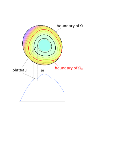
Figure 2. Depiction of $\Omega_{\circ}(\omega)$, the largest subset of $\Omega$ bounded by an $\omega$ level set. Note, the complement of $\Omega_{\circ}(\omega)$ contains level sets that intersect $\partial\Omega$. Also depicted is the plateau set $\Omega_{p}\subset\Omega$, a region where $\omega$=constant.

Now we make a moderate generalization about the regularity: Suppose that $\omega$ is Lipschitz continuous, i.e., $\omega\in C^{0,1}(\Omega)$. Then, $\omega$ has a classical gradient $\nabla\omega$ almost everywhere in $\Omega$ (see e.g. [33]), and $|\nabla\omega|$ is bounded. Note, $\omega$ may fail to have a classical $\nabla\omega$ on a measure-zero subset $\Omega_{s}\subset\Omega$, but for $\bm{x}\in\Omega_{s}$ we may define a set-valued generalized gradient (see [9]). With a Lipschitz continuous function $g:\mathbb{R}\rightarrow\mathbb{R}$ we can solve (3.1) by

$$\psi=g(\omega),\quad\theta=\vartheta(\omega),$$ (3.7)

where $\vartheta(\xi)=g(\xi)\xi-\int\!d\xi\,g(\xi)$. To meet the boundary condition $\psi|_{\partial\Omega}=0$, $g$ must satisfy

$$g(\omega(\bm{x}))=0\quad\forall\bm{x}\in\partial\Omega.$$ (3.8)

However, the solution (3.7) omits a different type of solution that emerges with a singularity of $\mathcal{J}(\omega)$: If $\omega$ has a “plateau,” i.e., $\omega=\omega_{0}$ (constant) in a finite region $\Omega_{p}\subseteq\Omega$ (see Fig. 2), the operator $\mathcal{J}(\omega)$ trivializes as $\mathcal{J}(\omega)=\{\omega_{0},\cdot\}=0$ in $\Omega_{p}$ (i.e., the “rank” drops to zero; recall the example of Sec. 1), and within $\Omega_{p}$ we can solve (3.1) by an arbitrary $\psi$ with $\theta=\omega_{0}\psi$. Notice that the solution (3.7) restricts $\psi=g(\omega_{0})$ = constant in $\Omega_{p}$. To remove this degeneracy, we abandon the continuity of $g$ and, for simplicity, assume that $\omega$ has only a single plateau. First we invoke the reversed form [cf.  (3.6)]:

$$\omega=f(\psi)\,,$$ (3.9)

where we assume that $f$ is a Lipschitz continuous monotonic function. Denoting $\vartheta(\eta)=\int\!d\eta\,f(\eta)$, we may write $\omega\nabla\psi=\nabla\vartheta(\psi)$, where the gradients on both sides evaluate classically almost everywhere in $\Omega$ if $\psi$ is Lipschitz continuous. If the function $f(\psi)$ is flat on some interval, $f(\psi)=\omega_{0}$ = constant for $\psi_{-}<\psi<\psi_{+}$, a plateau appears in the distribution of $\omega$. See Figs. 2 and 3(a). Since the present mission is to find $\psi$ for a given $\omega$, we transform (3.9) back to (3.7) with the definition $g=f^{-1}$. (In Sec. 4, however, we will seek an equilibrium $\omega$ that is characterized by a Casimir element, and then, the form (3.9) will be invoked again). A plateau in the graph of $f$ will, then, appear as a “jump” in the graph of $g$. See Fig. 3(b).

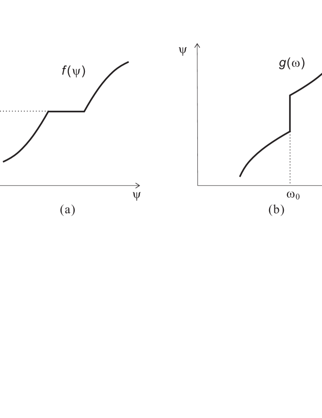
Figure 3. Depiction of the dual relationships between $\psi$ and $\omega$. (a) The relation $\omega=f(\psi)$ with the plateau singularity. (b) The singular (discontinuous) function $\psi=g(\omega)$ illustrating the kernel element that stems from a plateau of $\omega$.

We now allow the function $g(\omega)$ to have a jump at $\omega_{0}=\omega|_{\Omega_{p}}$. Formally we write $g(\omega)=g_{L}(\omega)+\alpha{Y}(\omega-\omega_{0})$, with $g_{L}(\omega)$ a Lipschitz continuous function, ${Y}(\omega-\omega_{0})$ the step function, and $\alpha$ a constant determining the width of the jump. We connect the graph of the step function by filling the gap between $\lim_{\omega\uparrow\omega_{0}}g(\omega)=\psi_{-}$ and $\lim_{\omega\downarrow\omega_{0}}g(\omega)=\psi_{+}=\psi_{-}+\alpha$. See Fig. 3(b). Since $g(\omega)$ is multi-valued at $\omega=\omega_{0}$, $\psi(\bm{x})=g(\omega(\bm{x}))$ is arbitrary in the range of $[\psi_{-},\psi_{+}]$, i.e. in $\Omega_{p}$. Choosing a sufficiently smooth $\psi$ in $\Omega_{p}$, we may assume $\psi\in H^{1}(\Omega)$.

Summarizing the above discussions (and making an obvious generalization), we have

Theorem 3.2.

Suppose that $\omega\in C^{0,1}(\Omega)$ and $\Omega_{\circ}(\omega)\neq\emptyset$. Then $\mathrm{Ker}(\mathcal{J}(\omega))$ contains nontrivial elements, and a part of them can be represented as

$$\psi=g(\omega),$$ (3.10)

where $g(\xi)$ is an arbitrary function that satisfies the boundary condition (3.8) and such that

$$g(\xi)=g_{L}(\xi)+\sum_{\ell=1}^{\nu}\alpha_{\ell}{Y}(\xi-\omega_{\ell}),$$ (3.11)

where $\omega_{\ell}$ denotes the height of a plateau of $\omega$, ${Y}(\xi)$ is the “filled” step function, and $\alpha_{\ell}$ is a constant.

Remark 3.3.

Notice that $\mathrm{Ker}(\mathcal{J}(\omega))$ is enlarged by the singular components $\alpha_{\ell}{Y}(\xi-\omega_{\ell})$ stemming from $\omega$ (the singular point in the phase space $H^{-1}(\Omega)$) that has plateaus $\omega=\omega_{\ell}$. Away from the singular point, the plateaus shrink to zero-measure sets in $\Omega$ and, then, $\psi=g(\omega)$ can no longer be a member of the domain of $\mathcal{J}(\omega)$. However, it is still a “hyperfunction solution” of $\{\omega,\psi\}=0$, since $\nabla\omega$ parallels the delta-function $\nabla\psi$ at $\omega=\omega_{\ell}$. The corresponding Casimir element, to be constructed in Sec. 3.2, is what we call a “singular Casimir element” (remember the elementary example discussed in Sec. 1; see also Fig. 1).

Remark 3.4.

In (3.11), the function $g(\xi)$ may be chosen arbitrarily to define an infinite number of kernel elements $\psi=g(\omega)$ satisfying (3.1). To find kernel elements (and in the following step of finding Casimir elements), we solve a linear equation $\mathcal{J}(\omega)\psi=0$ (and $\mathcal{J}(\omega)\partial_{\psi}C(\psi)=0$) for a given $\omega$; see Remark 1.2. In the analysis of “equilibrium points” (Sec. 4), however, we will relate $\psi\in\mathrm{Ker}(\mathcal{J}(\omega))$ and $\omega$ by another defining relation $-\Delta\psi=\omega$ so as to make $\psi$ the Clebsch potential of $\omega$ (see (2.12)). Then, $g(\xi)$ is provided as a data specifying a Casimir leaf on which we seek an equilibrium point.

Remark 3.5.

Clearly the form (3.11) of $g(\omega)$ is rather restrictive:

(i) In the plateau region, (3.1) has a wider class of solutions. In fact, $\psi$ may be an arbitrary $H^{1}$-class function whose range may exceed the interval $[\psi_{-},\psi_{+}]$. In this case, the graph of $g(\omega)$ has a “thorn” at $\omega_{0}$, and we may not integrate such a function to define a Casimir element $G(\omega)$. (See Sec. 3.2.)

(ii) In (3.11), we restrict the continuous part $g_{L}(\xi)$ to be Lipschitz continuous, by which $\psi=g(\omega)$ ($\omega\in C^{0,1}(\Omega)$) is assured of Lipschitz continuity (thus, $\psi\in H^{1}(\Omega)$). However, this condition may be weakened, depending on the specific $\omega$, i.e., it is only required that $g^{\prime}(\omega)\nabla\omega\in H^{1}(\Omega)$.

3.2. Construction of Casimir Elements

Our next mission is to “integrate” the kernel element $\psi\in\mathrm{Ker}(\mathcal{J}(\omega))$ as a function of $\omega$, and define a Casimir element $C(\omega)$, i.e., to find a functional $C(\omega)$ such that $\partial_{\omega}C(\omega)\in\mathrm{Ker}(\mathcal{J}(\omega))$. To this end, the parameterized $\psi$ of (3.10) will be used, where the function $g(\omega)$ may have singularities as described in Theorem 3.2. The central issue of this section, then, will be to consider an appropriate “generalized functional derivative” by which we can define “singular Casimir elements” pertinent to the singularities of the noncanonical Poisson operator $\mathcal{J}(\omega)$.

Let us start by considering a regular Casimir element generated by $g(\xi)\in C(\mathbb{R})$:

$$C_{G}(\omega)=\int_{\Omega}\!dx\,G(\omega)\,,$$ (3.12)

where $G(\xi):=\int\!d\xi\,g(\xi)$. The gradient of this functional can be readily calculated with the definition of Sec. 2.3: Perturbing $\omega$ by $\epsilon\tilde{\omega}$ results in

$$\delta C_{G}(\omega,\tilde{\omega})=\epsilon\int_{\Omega}\!dx\,g(\omega)\tilde{\omega}+O(\epsilon^{2})\,.$$

Hence, we obtain $\partial_{\omega}C_{G}(\omega)=g(\omega)$, proving that $C_{G}(\omega)$ of (3.12) is the Casimir element corresponding to $g(\omega)\in\mathrm{Ker}(\mathcal{J}(\omega))$.

Now we construct a singular Casimir element corresponding to a general $g(\omega)$ that may have “jumps” at the singularity of $\mathcal{J}(\omega)$, i.e., the plateaus of $\omega$. The formal primitive function $G(\xi)$ of such a $g(\xi)$ has “kinks” where the classical differential does not apply —this problem leads to the requirement of an appropriately generalized gradient of the functional $C_{G}(\omega)=\int_{\Omega}\!dx\,G(\omega)$ generated by a kinked $G(\xi)$.

Here we invoke the Clarke gradient [9], which is a generalized gradient for Lipschitz-continuous functions or functionals. Specifically, if $F:\mathbb{R}\rightarrow\mathbb{R}$, then the Clarke gradient of $F$ at $x$, denoted by $\tilde{\partial}_{x}F(x)$, is defined to be the convex hull of the set of limit points of the form

$$\lim_{j\rightarrow\infty}\partial_{x}F(x+\delta_{j})\quad{\rm with}\quad\lim_{j\rightarrow\infty}\delta_{j}=0.$$ (3.13)

Evidently, $\tilde{\partial}_{x}F(x)$ is equivalent to the classical gradient, $\partial_{x}F(x)$, if $F(x)$ is continuously differentiable in the neighborhood of $x$. Also, it is evident that a “kink” in $F$ yields $\tilde{\partial}_{x}F(x)$ with a graph that has a “jump” with the gap filled as depicted in Fig. 3(b). When $F(u)$ is a convex functional on a Hilbert space $X$, i.e. $F:X\rightarrow\mathbb{R}$, then $\tilde{\partial}_{u}F(u)$ is equal to the sub-differential:

$$\tilde{\partial}_{u}F:u\mapsto\{g{\,|\ }F(u+\delta)-F(u)\geq(g,u),~{}\forall\delta\in X\},$$ (3.14)

which gives the maximally monotone (i.e., the gap-filled) function [5]. For the purpose of Sec. 4, a monotonic $g(\xi)=\tilde{\partial}_{\xi}G(\xi)$ will be sufficient.

From the above, the following conclusion is readily deducible:

Corollary 3.6.

Suppose that $\omega\in C^{0,1}(\Omega)$ and $\Omega_{\circ}(\omega)\neq\emptyset$. By $g(\xi)$ satisfying (3.8) and (3.11), we define $G(\xi)$ such that $g(\xi)=\tilde{\partial}_{\xi}G(\xi)$. Then, $C_{G}(\omega)=\int_{\Omega}\!dx\,G(\omega)$ is a generalized Casimir element, i.e., $\tilde{\partial}_{\omega}C_{G}(\omega)\in\mathrm{Ker}(\mathcal{J}(\omega))$.

4. Extremal Points

4.1. Extremal Points and Casimir Elements

The Casimir element $C_{G}(\omega)$ naturally extends the set of extremal equilibrium points, the set of solutions of the dynamical system (2.19) that are both equilibrium solutions and energy-Casimir extremal points. This is done by including extremal points satisfying [cf. (1.9)]

$$\tilde{\partial}_{\omega}[H(\omega)+C_{G}(\omega)]\ni 0,$$ (4.1)

which explicitly gives

$$\mathcal{K}\omega\in-g(\omega).$$ (4.2)

Here we assume that $g(\xi)=\tilde{\partial}_{\xi}G(\xi)$ is a monotonic function, i.e., $G(\xi)$ is convex. Then, we may define a single-valued continuous function $f=(-g)^{-1}$ and rewrite (4.2), denoting $\varphi=\mathcal{K}\omega$, as

$$-\Delta\varphi=f(\varphi).$$ (4.3)

If $f(0)\neq 0$, (4.3) will determine a nontrivial ($\varphi\not\equiv 0$) equilibrium extremal point. Notice that $f(\xi)$ (or $g(\xi)=-f^{-1}(\xi)$ or $G=\int d\xi g(\xi)$) is a given function that specifies a Casimir leaf on which we seek an equilibrium point (see Remark 3.4). Here we prove the following existence theorem:

Theorem 4.1.

There exists a finite positive number $M$, determined only by the geometry of $\Omega$, such that if

$$L:=\inf_{\eta\in\mathbb{R}}\frac{|f(\eta)|}{|\eta|}<M,$$ (4.4)

then (4.3) has a solution $\varphi\in H^{1}_{0}(\Omega)$.

Proof.

We show the existence of the solution by Schauder’s fixed-point theorem (see for example [31, p. 20] and [1, p. 43]). First we rewrite (4.3) as

$$\omega=\mathcal{F}(\omega):=f(\mathcal{K}\omega),$$ (4.5)

where $\mathcal{K}$ is a compact operator on $L^{2}(\Omega)$ (cf.  (2.12)). Since $f\in C(\mathbb{R})$, $\mathcal{F}$ is a continuous compact map on $L^{2}(\Omega)$. We consider a closed convex subset

$$W_{\Lambda}=\{\omega{\,|\ }\|\omega\|\leq\Lambda\}~{}\subset L^{2}(\Omega),$$

where $\|\omega\|$ is the norm of $L^{2}(\Omega)$ and the parameter $\Lambda$ will be determined later. We show that the compact map $\mathcal{F}$ has a fixed point in $W_{\Lambda}$. By Poincaré’s inequality, we have, for $\varphi\in H^{1}_{0}(\Omega)$,

$$\|\varphi\|\leq c_{1}\|\nabla\varphi\|,$$

where $c_{1}$ is a positive number that is determined by the geometry of $\Omega$. For $\bm{u}=\nabla\varphi\times\bm{e}\in L^{2}_{\sigma}(\Omega)\cap H^{1}(\Omega)$, we have

$$\|\bm{u}\|\leq c_{2}\|\nabla\times\bm{u}\|,$$

where $c_{2}$ is also a positive number determined by the geometry of $\Omega$. Here $\|\bm{u}\|=\|\nabla\varphi\|$ and $\|\nabla\times\bm{u}\|=\|\Delta\varphi\|$. Hence, denoting $c_{p}=c_{2}c_{1}+c_{2}+1$, we have

$$\|\varphi\|_{H^{2}}:=\|\varphi\|+\|\nabla\varphi\|+\|\Delta\varphi\|\leq c_{p}\|\Delta\varphi\|.$$

By Sobolev’s inequality, we have

$$\sup_{\Omega}|\varphi|\leq c_{s}\|\varphi\|_{H^{2}},$$

where $c_{s}$ is again a positive number determined by the geometry of $\Omega$. Summarizing these estimates, we have, for $\omega\in W_{\Lambda}$,

$$\sup_{\Omega}|\mathcal{K}\omega|\leq c_{s}c_{p}\|\omega\|\leq c_{s}c_{p}\Lambda.$$

For an arbitrary positive number $\delta$, there is a finite number $\eta^{*}$ such that $|f(\pm\eta^{*})|\leq(L+\delta)|\eta^{*}|$. If we choose $\Lambda=|\eta^{*}|/(c_{s}c_{p})$, then by the monotonicity of $f(\eta)$, we find

$$\sup_{\Omega}|f(\mathcal{K}\omega)|\leq(L+\delta)|\eta^{*}|=(L+\delta)c_{s}c_{p}\Lambda,$$ (4.6)

and, upon denoting $|\Omega|:=\int_{\Omega}\!dx$, we obtain

$$\|f(\mathcal{K}\omega)\|\leq|\Omega|^{1/2}(L+\delta)c_{s}c_{p}\Lambda=(L+\delta)\Lambda/M\,,$$

where

$$M:=\frac{1}{|\Omega|^{1/2}c_{s}c_{p}}\,.$$ (4.7)

If $(L+\delta)\leq M$, we estimate $\|f(\mathcal{K}\omega)\|\leq\Lambda$, and thus $\mathcal{F}$ maps $W_{\Lambda}$ into $W_{\Lambda}$. Therefore, $\mathcal{F}$ has a fixed-point in $W_{\Lambda}$. If $W_{\Lambda}$ contains a fixed point, then an arbitrary $W_{\Lambda^{\prime}}$ with $\Lambda^{\prime}>\Lambda$ contains a fixed-point. Since $\delta$ is arbitrary, $L<M$ is the sufficient condition for the existence of a fixed point. ∎

Corollary 4.2.

If $L=|f(\eta^{*})|/|\eta^{*}|>0$ for some finite $\eta^{*}$, then we may assume $\delta=0$ in (4.6), and the solvability condition (4.4) can be modified to be $L\leq M$.

The bound $M$ defined by (4.7) is related to the eigenvalue of $-\Delta=\mathcal{K}^{-1}$. On the other hand, the constant $L$ defined by (4.4) is a property of the Casimir element. As noted above, because of the homogeneity of (1.4), there is at least a one-parameter family of Casimir elements and the choice of a multiplicative constant reciprocally scales $L$. This provides an arbitrary parameter multiplying the Casimir element in the determining equation (4.1), and such a parameter may be considered to be an “eigenvalue” characterizing the stationary point. The no-solution example of the next section will reveal the “nonlinear property” of this eigenvalue problem.

4.2. No-Solution Example

Here we present a class of examples that violate the solvability condition proposed in Theorem 4.1. This demonstrates that finding Casimir elements that generalize the extremal equation (4.3), does not automatically extend the set of extremal equilibria, since the resulting elliptic equation may not have a solution. This is demonstrated by the following two propositions.

Proposition 4.3.

Let $f(\varphi)$ have the form

$$f(\varphi)=\lambda_{1}\varphi+\vartheta(\varphi),$$ (4.8)

where $\lambda_{1}$ is the first eigenvalue of $-\Delta=\mathcal{K}^{-1}$ and $\vartheta>0$. Then, (4.3) does not have a solution.

Proof.

We denote by $\phi_{1}$ the eigenfunction corresponding to the eigenvalue $\lambda_{1}$. Upon taking the inner product of (4.3) with $\phi_{1}$, we obtain

$$(-\Delta\varphi,\phi_{1})=(\lambda_{1}\varphi,\phi_{1})+(\vartheta(\varphi),\phi_{1}).$$ (4.9)

The left-hand-side of (4.9) satisfies $(-\Delta\varphi,\phi_{1})=(\varphi,-\Delta\phi_{1})=(\lambda_{1}\varphi,\phi_{1})$, which cancels the first term on the right-hand-side, leaving $(\vartheta(\varphi),\phi_{1})=0$. However, this is a contradiction, because $\phi_{1}>0$ (or $<0$ if otherwise normalized) on $\Omega$ and, by the assumption, $\vartheta(\varphi)>0$. ∎

The above result is easily generalized as follows:

Proposition 4.4.

Suppose that

$$f(\varphi)=\lambda_{j}\varphi+\vartheta(\varphi),$$ (4.10)

where $\lambda_{j}$ is any eigenvalue of $-\Delta$ and $0<A<\vartheta(\varphi)<B$, for some $A$ and $B$. Let $\phi_{j}$ be the eigenfunction corresponding to $\lambda_{j}$. Since $\phi_{j}$ may not have a definite sign in $\Omega$, we divide $\Omega$ into $\Omega_{+}=\{x\in\Omega{\,|\ }\phi_{j}(x)>0\}$ and $\Omega_{-}=\{x\in\Omega{\,|\ }\phi_{j}(x)<0\}$, and define

$$P_{+}=\int_{\Omega_{+}}\!\!dx\,\phi_{j}\,,\quad P_{-}=-\int_{\Omega_{-}}\!\!dx\,\phi_{j}\quad({\rm both}\ \geq 0)$$

If $P_{+}\neq P_{-}$, (4.3) does not have a solution for some ranges of $A$ and $B$.

Proof.

As shown in the proof of Proposition 4.4, a solution of (4.3) must satisfy

$$(\vartheta(\varphi),\phi_{j})=\int_{\Omega_{+}}\!\!dx\,\vartheta(\varphi)\phi_{j}+\int_{\Omega_{-}}\!\!dx\,\vartheta(\varphi)\phi_{j}=0\,.$$

By assumption, we have

$$A\phi_{j}<\vartheta(\varphi)\phi_{j}<B\phi_{j}\quad \mathrm{in} \Omega_{+},$$

$$A\phi_{j}>\vartheta(\varphi)\phi_{j}>B\phi_{j}\quad \mathrm{in} \Omega_{-}.$$

Hence, the inequalities

$$AP_{+}-BP_{-}<0<BP_{+}-AP_{-}$$

must hold, i.e.,

$$A/B<P_{-}/P_{+},$$ (4.11)

$$B/A>P_{-}/P_{+}.$$ (4.12)

However, if $P_{-}/P_{+}<1$, and $A$ and $B$ are such that $1>A/B>P_{-}/P_{+}$, then there is a contradiction with (4.11). Similarly, if $P_{-}/P_{+}>1$, and $A$ and $B$ are such that $1<B/A<P_{-}/P_{+}$, then there is a contradiction with (4.12). ∎

5. Concluding Remarks

After establishing some mathematical facts about the Hamiltonian form of the Euler equation of two-dimensional incompressible inviscid flow, we studied the center of the Poisson algebra, i.e., the kernel of the noncanonical Poisson operator $\mathcal{J}(\omega)$. Casimir elements $C(\omega)$ were obtained by “integrating” the “differential equation”

$$\mathcal{J}(\omega)\partial_{\omega}C(\omega)=0\,.$$

For finite-dimensional systems with phase space coordinate $z$, this amounts to an analysis of $\mathcal{P}:=\mathcal{J}(z)\partial_{z}$, a linear partial differential operator, and nontriviality can arise from a singularity of $\mathcal{P}$, whence an inherent structure emerges. Recall the simple example given in Sec. 1 where $\mathcal{P}=ix\partial_{x}$ was seen to generate the hyperfunction Casimir $C(x)=Y(x)$. For finite-dimensional systems the theory naturally finds its way to algebraic analysis: in the language of D-module theory, Casimir elements constitute $\mathrm{Ker}(\mathcal{P})=\mathrm{Hom}_{\mathcal{D}}(\mathrm{Coker}(\mathcal{P}),F)$, where $\mathcal{D}$ is the ring of partial differential operators and $F$ is the function space on which $\mathcal{P}$ operates, and $\mathrm{Coker}(\mathcal{P})=\mathcal{D}/\mathcal{D}\mathcal{P}$ is the D-module corresponding to the equation $\mathcal{P}C(\omega)=0$. However, in the present study $\omega$ is a member of an infinite-dimensional Hilbert space, thus $\mathcal{P}$ may be regarded as an infinite-dimensional generalization of linear partial differential operators. From the singularity of such an infinite-dimensional (or functional) differential operator $\mathcal{P}=\mathcal{J}(\omega)\partial_{\omega}$, we unearthed singular Casimir elements, and to justify the operation of $\mathcal{P}$ on singular elements, we invoked a generalized functional derivative (Clarke differential or sub-differential) that we denoted by $\tilde{\partial}_{\omega}$.

For infinite-dimensional systems, we cannot “count” the dimensions of $\mathrm{Ker}(\mathcal{P})$ and $\mathrm{Ker}(\mathcal{J})$. It is, however, evident that $\mathrm{dim-Ker}(\mathcal{P})<\mathrm{dim-Ker}(\mathcal{J})$, if $\mathcal{J}$ has singularities, i.e., singularities create “nonintegrable” elements of $\mathrm{Ker}(\mathcal{J})$. As shown in Theorem 3.2, a plateau in $\omega$ causes a singularity of $\mathcal{J}(\omega)$ and generates new elements of $\mathrm{Ker}(\mathcal{J}(\omega))$, which can be integrated to produce singular Casimir elements (Corollary 3.6). However, as noted in Remark 3.5(i), more general elements of $\mathrm{Ker}(\mathcal{J}(\omega))$ that are not integrable may stem from a plateau singularity. Moreover, we had to assume Lipschitz continuity for $\omega$ to obtain an explicit relation between $\psi\in\mathrm{Ker}(\mathcal{J}(\omega))$ and $\omega$ – otherwise we could not integrate $\psi$ with respect to $\omega$ to construct a Casimir element. In the general definition of $\mathcal{J}(\omega)$, however, $\omega$ may be nondifferentiable (we assumed only continuity), and then, a general $\psi\in\mathrm{Ker}(\mathcal{J}(\omega))$ may not have an integrable relation to $\omega$ (see Lemma 3.1).

In Sec. 4 we solved the equation

$$\tilde{\partial}_{\omega}[H(\omega)+C(\omega)]\ni 0$$

for $\omega$, where the solution $\omega$ gave an equilibrium point of the dynamics induced by a Hamiltonian $H(\omega)$. A singular (kinked) Casimir yielded a multivalued (set-valued) gradient $\tilde{\partial}_{\omega}C(\omega)$, encompassing an infinite-dimensional solution stemming from the plateau singularity. This arose because in the plateau of $\omega$, $\psi\in\mathrm{Ker}(\mathcal{J}(\omega))$ is freed from $\omega$ and may distribute arbitrarily. The component $g_{L}(\omega)$ of the Casimir $C(\omega)$ of (3.11) represents explicitly the regular “dimensions” of $\mathrm{Ker}(\mathcal{J}(\omega))$. In contrast, the undetermined dimensions pertinent to the singularity $\omega=\omega_{0}$ are “implicitly” included in the step-function component of (3.11), or in the kink of $C(\omega)$. However, for a given Hamiltonian $H(\omega)$, i.e. a given dynamics, a specific relation between $\varphi\in\tilde{\partial}_{\omega}C(\omega)$ and $\omega$ emerges.

Theorem 4.1 of Sec. 4.1 and the nonexistence examples of Sec. 4.2 may not be new results in the theory of elliptic partial differential equations, but they do help delineate the relationship between Hamiltonians and Casimir elements, viz.  that Casimir elements alone do not determine the extent of the set of equilibrium points. In the present paper, we did not discuss the bifurcation of the equilibrium points; the reader is referred to [1] for a presentation of the actual state of the studies of semilinear elliptic problems and several techniques in nonlinear analysis (see also [31] and [19]). We also note that we have excluded nonmonotonic $g(\omega)$ that will make $f(\varphi)$ multivalued or, more generally, equations like $\Phi(\Delta\varphi,\varphi)=0$; cf. (3.6). For fully nonlinear elliptic partial differential equations, the reader is referred to [31, 30, 13, 7, 8].

Appendix A. On the Poisson operator in terms of the velocity field $\bm{u}\in L^{2}_{\sigma}(\Omega)$

Here we formulate the Euler equation, for both $n=2$ and 3, as an evolution equation in $L_{\sigma}^{2}(\Omega)$ (see Sec. 2.1), and discuss the Poisson operator $\mathcal{J}({\bm{u}})$ in this space. This differs from the formulation of Sec. 2 in that the state variable here is the velocity field $\bm{u}\in L_{\sigma}^{2}(\Omega)$ instead of the vorticity $\omega$. As noted in Sec. 2.1, $L_{\sigma}^{2}(\Omega)$ is a closed subspace of $L^{2}(\Omega)$, and we have the orthogonal decomposition (2.7). We denote by $P_{\sigma}$ the orthogonal projection onto $L_{\sigma}^{2}(\Omega)$. Upon applying $P_{\sigma}$ to the both sides of (2.4), we obtain

$$\partial_{t}\bm{u}=-P_{\sigma}(\nabla\times\bm{u})\times\bm{u},$$ (5.1)

which is interpreted as the evolution equation in $L^{2}_{\sigma}(\Omega)$, where the incompressibility condition (2.2) and the boundary condition (2.3) are implied by $\bm{u}\in L^{2}_{\sigma}(\Omega)$.

For $\bm{u}\in L^{2}_{\sigma}(\Omega)$, the Hamiltonian is, of course, the kinetic energy

$$H(\bm{u})=\frac{1}{2}\|\bm{u}\|^{2}\,.$$ (5.2)

Fixing a sufficiently smooth $\bm{u}$ acting as a parameter, viz.  $\nabla\times\bm{u}\in C(\Omega)$, we define for $\bm{v}\in L^{2}_{\sigma}(\Omega)$ the following the noncanonical Poisson operator:

$$\mathcal{J}({\bm{u}})\bm{v}=-P_{\sigma}(\nabla\times\bm{u})\times\bm{v}\,.$$ (5.3)

As a linear operator (recall Remark 1.2 of Sec. 1), $\mathcal{J}(\bm{u})$ consists of the vector multiplication by $(\nabla\times\bm{u})$ followed by projection with $P_{\sigma}$. Evidently, $\mathcal{J}({\bm{u}})$ is antisymmetric:

$$(\mathcal{J}({\bm{u}})\bm{v},\bm{v}^{\prime})=-(\bm{v},\mathcal{J}({\bm{u}})\bm{v}^{\prime})\quad\forall\bm{v},\bm{v}^{\prime}\in L_{\sigma}^{2}(\Omega).$$

In fact, for every fixed smooth $\bm{u}$, $i\mathcal{J}(\bm{u})$ is a self-adjoint bounded operator in $L^{2}_{\sigma}(\Omega)$.

With the $H(\bm{u})$ of (5.2), the $\mathcal{J}(\bm{u})$ of (5.3), and the gradient $\partial_{\bm{u}}$ (see Sec. 2.3), we may write (5.1) as

$$\partial_{t}\bm{u}=\mathcal{J}({\bm{u}})\partial_{\bm{u}}H(\bm{u}).$$ (5.4)

Assuming $n=2$, which we do henceforth, by Lemma 2.1 we may put $\bm{u}=\nabla\varphi\times\bm{e}$ and $\omega=-\Delta\varphi$ with $\varphi\in H_{0}^{1}(\Omega)$. Fixing $\omega\in C(\Omega)$ as a parameter, and putting $\bm{v}=\nabla\psi\times\bm{e}$ with $\psi\in H_{0}^{1}(\Omega)$, we may write

$$\mathcal{J}({\bm{u}})\bm{v}=-P_{\sigma}\left[\omega\bm{e}\times(\nabla\psi\times\bm{e})\right]=-P_{\sigma}\left[\omega\nabla\psi\right].$$

By (2.7), $\bm{v}\in\mathrm{Ker}(\mathcal{J}({\bm{u}}))$ iff

$$\omega\nabla\psi=\nabla\theta\quad\exists\theta\in H^{1}(\Omega),$$ (5.5)

which is equivalent to (3.1). Arguing just like in Sec. 3.1, we find solutions of (5.5) of the form

$$\psi=g(\omega).$$ (5.6)

The Casimir element constructed from (5.6) is

$$C_{G}(\bm{u})=\int_{\Omega}\!dx\,G(\bm{e}\cdot\nabla\times\bm{u})=\int_{\Omega}\!dx\,G(\omega)\,.$$ (5.7)

Perturbing $\bm{u}$ by $\epsilon\tilde{\bm{u}}$ and restricting $\bm{n}\cdot\tilde{\bm{u}}=0$ on $\partial\Omega$ yields $\delta\omega=\epsilon\bm{e}\cdot\nabla\times\tilde{\bm{u}}$, and

$$\delta C_{G}(\bm{u};\tilde{\bm{u}}) = \epsilon\int_{\Omega}\!dx\,G^{\prime}(\omega)\bm{e}\cdot\nabla\times\tilde{\bm{u}}+O(\epsilon^{2})$$

$$= \epsilon\int_{\Omega}\!dx\,\nabla G^{\prime}(\omega)\times\bm{e}\cdot\tilde{\bm{u}}+O(\epsilon^{2}).$$

Hence, upon denoting $g(\omega)=G^{\prime}(\omega)$ we obtain

$$\partial_{\bm{u}}C_{G}(\bm{u})=\nabla g(\omega)\times\bm{e}\,.$$ (5.8)

By (5.6), it is evident that $\mathcal{J}({\bm{u}})\partial_{\bm{u}}C_{G}(\bm{u})=-P_{\sigma}[\omega\nabla g(\omega)]=0$, confirming that $\partial_{\bm{u}}C_{G}(\bm{u})\in\mathrm{Ker}(\mathcal{J}(\bm{u}))$.

Since here, $H(\bm{u})=\|\bm{u}\|^{2}/2$, we may find an equilibrium point by solving $\bm{u}=-\partial_{\bm{u}}C_{G}(\bm{u})$ (c.f.  Sec. 1, Eq. (1.9)).

References

- [1] A. Ambrosetti and A. Malchiodi, Nonlinear analysis and semilinear elliptic problems, Cambridge Studies in Advanced Mathematics 104, Cambridge Univ. Press, ,2007.
- [2] V. I. Arnold, On an a priori estimate in the theory of hydrodynamic stability, Amer. Math. Soc. Transl. 19 (1969), 267–269.
- [3] V. I. Arnold, Sur la géometrie différentielle des groupes de Lie de dimension infinie et ses applications à l’hydrodynamique des fluides parfaits, Ann. Inst. Fourier (Grenoble) 16 (1966), 319–361.
- [4] V. I. Arnold, The Hamiltonian nature of the Euler equation in the dynamics of a rigid body and of an ideal fluid, Usp. Mat. Nauk 24(3) (1969), 225–226.
- [5] H. Brézis, Opérateurs maximaux monotones et semi-groupes de contractions dans les espace de Hilbert. North-Holland, 1973.
- [6] H. Brézis, Functional analysis, Sobolev spaces and partial differential equations, Springer, 2011.
- [7] L. Caffarelli and X. Cabré, Fully nonlinear elliptic equations, AMS Colloquium Publ. 43, AMS, 1995.
- [8] L. Caffarelli and J. Salazar, Solutions of fully nonlinear elliptic equations with patches of zero gradient: existence, regularity and convexity of level curves, Trans. AMS 354 (2002), 3095–3115.
- [9] F. H. Clarke, Generalized gradients and applications, Trans. Amer. Math. Soc. 205 (1975), 247–262.
- [10] A. Clebsch, Über eine allgemeine Transformation der hydrodynamischen Gleichungen, Z. Reine Angew. Math. 54 (1857), 293–312.
- [11] A. Clebsch, Über die Integration del hydrodynamischen Gleichungen, Z. Reine Angew. Math. 56 (1859), 1–10.
- [12] C. Eckart, Variation principles of hydrodynamics, Phys. Fluids 3 (1960), 421–427.
- [13] L. C. Evans, Partial differential equations (2nd ed.), AMS, 2010.
- [14] T. Kato, On classical solutions of the two-dimensional non-stationary Euler equation, Arch. Rational Mech. Anal. 25 (1967), 188–200.
- [15] B. Khesin and R. Wendt, The geometry of infinite-dimensional groups, Springer, 2009.
- [16] G. Kirchhoff, Vorlesungen über Mathematische Physik, Mechanik c. XX, Leipzig (1867).
- [17] M. D. Kruskal and C. Oberman, On the stability of plasma in static equilibrium, Phys Fluids 1 (1958), 275–280.
- [18] J. L. Lagrange, Mécanique analytique, Desaint, 1788.
- [19] P. L. Lions, On the existence of positive solutions of semilinear elliptic equations, SIAM Rev. 24 (1982), 441–467.
- [20] P. J. Morrison and J. M. Greene, Noncanonical Hamiltonian density formulation of hydrodynamics and ideal magnetohydrodynamics, Phys. Rev. Lett. 45 (1980), 790–794.
- [21] P. J. Morrison, The Maxwell-Vlasov equations as a continuous hamiltonian system, Phys. Lett. A 80 (1980), 383–386.
- [22] P. J. Morrison, Hamiltonian field description of two-dimensional vortex fluids an guiding center plasmas, Princeton University Plasma Physics Laboratory Report, PPPL-1783 (1981); Available as American Institute of Physics Document No. PAPS-PFBPE-04-771-24.
- [23] P. J. Morrison, Hamiltonian field description of one-dimensional Poisson-Vlasov equation, Princeton University Plasma Physics Laboratory Report, PPPL-1788 (1981); Available as American Institute of Physics Document No. PAPS-PFBPE-04-771-14.
- [24] P. J. Morrison, in Mathematical Methods in Hydrodynamics and Integrability in Related Dynamical Systems, AIP Conference Proceedings No. 88, edited by M. Tabor and Y. Treve (AIP, New York, 1982), p. 13.
- [25] P. J. Morrison and D. Pfirsch, Free-energy expressions for Vlasov equilibria, Phys. Rev. A 40 (1989), 3898–3910.
- [26] P. J. Morrison, Hamiltonian description of the ideal fluid, Rev Mod Phys. 70 (1998), 467–521.
- [27] P. J. Morrison, Hamiltonian fluid mechanics, in Encyclopedia of Mathematical Physics, vol. 2, (Elsevier, Amsterdam, 2006) p. 593.
- [28] V. Narayanan and P. J. Morrison, Rank change in Poisson dynamical systems, arXiv:1302.7267 [math-ph].
- [29] W. A. Newcomb, Lagrangian and Hamiltonian methods in magnetohydrodynamics, Nucl. Fusion: Supplement, part 2 (1962), 451–463.
- [30] L. Nirenberg, Variational and topological methods in nonlinear problems, Bulletin AMS 4 (1981), 267–302.
- [31] L. Nirenberg, Topics in nonlinear functional analysis (New ed.), Courant Lecture Notes in Mathematics, ISSN1529-9031;6 (2001).
- [32] P. J. Olver, A nonlinear Hamiltonian structure for the Euler equations, J. Math. Anal. Appl. 89 (1982), 233–250.
- [33] E. M. Stein, Singular integrals and differentiability properties of functions, Princeton Math. Ser. no. 30, Princeton Univ. Press, 1970.
- [34] Z. Yoshida, Clebsch parameterization: basic properties and remarks on its applications, J. Math. Phys. 50 (2009), 113101 1-16.
- [35] V. E. Zakharov and E. A. Kuznetsov, Variational principle and canonical variables in magnetohydrodynamics, Sov. Phys. Dokl. 15(10) (1971), 913-914.