Cooperative Estimation of 3D Target Motion via Networked Visual Motion Observer

Abstract

This paper investigates cooperative estimation of 3D target object motion for visual sensor networks. In particular, we consider the situation where multiple smart vision cameras see a group of target objects. The objective here is to meet two requirements simultaneously: averaging for static objects and tracking to moving target objects. For this purpose, we present a cooperative estimation mechanism called networked visual motion observer. We then derive an upper bound of the ultimate error between the actual average and the estimates produced by the present networked estimation mechanism. Moreover, we also analyze the tracking performance of the estimates to moving target objects. Finally the effectiveness of the networked visual motion observer is demonstrated through simulation.

I Introduction

A visual sensor network [1, 2] is a kind of wireless sensor network consisting of spatially distributed smart cameras with communication and computation capability. Unlike other sensors measuring values such as temperature and pressure, vision sensors do not provide explicit data but combining image processing techniques or human operators gives rich information on situation awareness such as what happens, what a target is, where it is and where it bears. Due to their nature, visual sensor networks are useful in environmental monitoring, surveillance, target tracking and entertainment and are expected as a component of sustainable infrastructures.

A lot of research works have been devoted to fusing control techniques with visual information so-called visual feedback control or images in the loop [3]–[9]. The motivating scenarios of the fusion currently spread over the robotic systems into security and surveillance systems, medical imaging procedures, human-in-the-loop systems and even understanding biological perceptual information processing. Driven by the technological innovations of the smart wearable cameras, the aforementioned networked vision system also emerges as a challenging new application field of the visual feedback control and estimation.

In this paper, we focus on estimation of 3D rigid body motion as in [7]–[9], and reconsider the problem not for a single camera system but for the networked vision systems. In particular, we aim at an extension of [8] from the single camera to visual sensor networks, where the paper [8] presents a vision-based observer called visual motion observer [9] estimating 3D target object motion from 2D vision data. In visual sensor networks, it is expected that not only an estimate is produced but also the vision cameras cooperate with each other in an efficient manner, which brings us new theoretical challenges. The advantages of cooperation are: (i) accurate estimation by integrating rich information, (ii) tolerance against obstruction, misdetection in image processing and sensor failures and (iii) wide vision and elimination of blind areas by fusing images of a scene from a variety of viewpoints. To tackle such distributed estimation problems, cooperative control as in [10]–[15] provides useful methodologies. In this paper, we especially focus on passivity-based cooperative control schemes investigated in [12]–[15].

Cooperative estimation for sensor networks has been addressed in [16]–[24]. The main objective of these researches is averaging the local measurements or local estimates among sensors in a distributed fashion in order to improve estimation accuracy. For this purpose, most of the works utilize the consensus protocol [10] in the update of the local estimates. While [16, 17] assume that parameters to be estimated are fixed, [18]–[24] address estimation of dynamic parameters assuming that the parameters follow some dynamical system. Among them, [18]–[22] execute a large number of consensus iterations between each update of estimates, which is hardly applicable to dynamic estimation problems except for the case of slow dynamics. Meanwhile, [23] and [24] present estimation algorithms without using such iterations. Unfortunately, however, most of these algorithms are not applicable to our problem since the object’s pose takes values in a non-Euclidean space and the consensus scheme on a vector space [10] does not work there.

Meanwhile, average computation in the group of rotations is tackled by [17], [25], [26]. The paper [25] defines two types average rotations, Euclidean and Riemannian means, and derives their fundamental properties. Reference [26] presents a computational algorithm of the Riemannian mean and analyzes its convergence. The paper [17] presents a distributed version of the algorithm in [26] based on the consensus protocol [10], which is motivated by the visual sensor networks. However, [17] focuses on averaging by assuming that the target orientations are obtained a priori and the scheme cannot be essentially extended to dynamic estimation problems.

In this paper, we present a novel cooperative estimation mechanism called networked visual motion observer. We consider the situation where multiple smart vision cameras capture a group of target objects. Under the situation, the objective of the present estimation mechanism is to meet two requirements simultaneously: averaging for static objects, which means gaining estimates close to an average of multiple target objects’ poses, and tracking to moving target objects, which means that the estimates track the moving average within a bounded error. Namely, the present mechanism deals with both static and dynamic estimation problems. For this purpose, we first present the networked visual motion observer, which consists of the visual feedback and mutual feedback from neighboring vision cameras, based on the passivity-based visual motion observer [8] and the passivity-based pose synchronization law presented in [15].

We next evaluate the averaging performance attained by the networked visual motion observer. For this purpose, we define a notion of approximate averaging by using the ultimate error between the actual average and the estimates produced by the present observer. Then, we derive an upper bound of the ultimate error, whose partial solution is already given in [27, 28] and this paper provides its generalized version. The result gives us an insight into the gain selection such that average estimation becomes accurate if mutual feedback is much stronger than visual feedback.

We moreover evaluate the tracking performance of the estimates to moving target objects. Here, we view the body velocities of the target objects as a disturbance of the total networked system and evaluate the ultimate distance from the estimates to the average. We see from the result an insight that choosing a large visual feedback gain results in a good tracking performance.

Finally, we demonstrate the effectiveness of the present networked visual motion observer and validity of the theoretical results through simulation.

The organization of this paper is as follows. Section II explains the situation under consideration in this paper and formulates the visual sensor networks together with the objective to be met. In Section III, after introducing the visual motion observer [8], we present the networked visual motion observer. Section IV clarifies accuracy of the average estimation when the present estimation mechanism is applied to the network of vision cameras. Section V clarifies the tracking performance of the estimates when the target objects are moving. Verifications through simulation are shown in Section VI. Finally, Section VII draws conclusions.

We finally give some notations used in this paper, where the readers are recommended to refer to [3] for details on the terminologies. Throughout this paper, we use the notation $e^{\hat{\xi}_{ab}\theta_{ab}}\in{\cal{R}}^{3\times 3}$ to represent the rotation matrix of a frame $\Sigma_{b}$ relative to a frame $\Sigma_{a}$, which is orthogonal with unit determinant and hence an element of the Lie group $SO(3):=\{R\in{\cal{R}}^{3\times 3}|\ R^{T}R=I_{3}\mbox{ and }\det(R)=+1\}$. The vector $\xi_{ab}\in{\cal{R}}^{3}$ specifies the rotation axis and $\theta_{ab}\in{\cal{R}}$ is the rotation angle. For simplicity we use ${\xi}\theta_{ab}$ to denote ${\xi}_{ab}\theta_{ab}$. The configuration space of the rigid body motion is the product space $SE(3):={\cal{R}}^{3}\times SO(3)$. We use the $4\times 4$ matrix $g_{ab}=\left[\begin{array}[]{cc}e^{\hat{\xi}\theta_{ab}}&p_{ab}\cr 0&1\end{array}\right]$ as the homogeneous representation of $g_{ab}=(p_{ab},e^{\hat{\xi}\theta_{ab}})\in SE(3)$ describing the configuration of $\Sigma_{b}$ relative to $\Sigma_{a}$. The notation ‘$\wedge$’ is the operator such that $\hat{a}b=a\times b$ for the vector cross-product $\times$, i.e. $\hat{a}$ is a $3\times 3$ skew-symmetric matrix. The vector space of all $3\times 3$ skew-symmetric matrices is denoted by $so(3)$. The notation ‘$\vee$’ denotes the inverse operator to ‘$\wedge$’. Similarly to the definition of $so(3)$, we define $se(3):=\{(v,\hat{\omega}):v\in{\cal{R}}^{3},\hat{\omega}\in so(3)\}$. In homogeneous representation, we write an element $V:=(v,\omega)$ as $\hat{V}=\left[\begin{array}[]{cc}\hat{\omega}&v\cr 0&0\end{array}\right]$.

II Preparation for Visual Sensor Networks

Let us consider the situation where $n$ vision cameras ${\mathcal{V}}:=\{1,\cdots,n\}$ with communication and computation capability see a group of target objects $\{o_{i}\}_{i\in{\mathcal{V}}}$ (Fig. 2), where each vision camera $i\in{\mathcal{V}}$ captures object $o_{i}$ on its image plane. Throughout this paper, we use the pinhole-type vision cameras with perspective projection [3] as in Fig. 2. Note however that all of the subsequent discussions are applicable to panoramic cameras through the modifications in [29].

In this paper, we address estimation of average motion of the objects $\{o_{i}\}_{i\in{\mathcal{V}}}$. The problem includes a scenario such that all the cameras see a common single target object but the pose consistent with vision data differs from camera to camera due to incomplete localization and parametric uncertainties. Under such a situation, averaging the contaminated poses is a way to improve estimation accuracy [20].

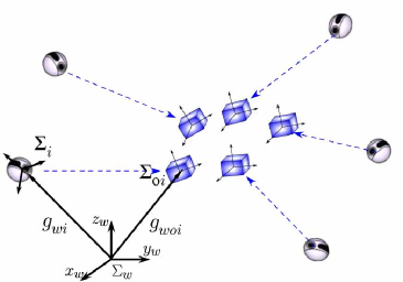
Figure 1: Visual Sensor Networks

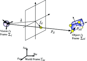
Figure 2: Vision Camera Model

II-A Rigid Body Motion

Let the coordinate frames $\Sigma_{w}$, $\Sigma_{i}$ and $\Sigma_{o_{i}}$ represent the world frame, the $i$-th vision camera frame, and the frame of object $o_{i}$, respectively. The pose of vision camera $\Sigma_{i}$ and object $\Sigma_{o_{i}}$ relative to the world frame $\Sigma_{w}$ are denoted by $g_{wi}=(p_{wi},e^{\hat{\xi}\theta_{wi}})\in SE(3)$ and $g_{wo_{i}}=(p_{wo_{i}},e^{\hat{\xi}\theta_{wo_{i}}})\in SE(3)$. Then, the pose of $\Sigma_{o_{i}}$ relative to $\Sigma_{i}$, denoted by $g_{io_{i}}=(p_{io_{i}},e^{\hat{\xi}\theta_{io_{i}}})\in SE(3)$, can be represented as $g_{io_{i}}=g_{wi}^{-1}g_{wo_{i}}$.

We next define the body velocity of object ${o_{i}}$ relative to the world frame $\Sigma_{w}$ as $V_{wo_{i}}^{b}=(v_{wo_{i}},\omega_{wo_{i}})\in{\cal{R}}^{6}$, where $v_{wo_{i}}$ and $\omega_{wo_{i}}$ respectively represent the linear and angular velocities of the origin of $\Sigma_{o_{i}}$ relative to $\Sigma_{w}$ [3]. Similarly, vision camera $i$’s body velocity relative to $\Sigma_{w}$ will be denoted as $V_{wi}^{b}=(v_{wi},\omega_{wi})\in{\cal{R}}^{6}$.

By using the body velocities $V_{wi}^{b}$ and $V_{wo_{i}}^{b}$, the motion of the relative pose $g_{io_{i}}$ is written as

$$\dot{g}_{io_{i}}=-\hat{V}_{wi}^{b}g_{io_{i}}+g_{io_{i}}\hat{V}_{wo_{i}}^{b}$$ (1)

[3]. Equation (1) is called relative rigid body motion whose block diagram is depicted in Fig. 4.

II-B Visual Measurement

In this subsection, we define visual measurements of each vision camera which is available for estimation. We assume that each target object has $m$ feature points and each vision camera can extract them from the vision data by using some techniques like [30]. The position vectors of the target object $i$’s $l$-th feature point relative to $\Sigma_{o_{i}}$ and $\Sigma_{i}$ are denoted by $p_{o_{i}l}\in{\cal{R}}^{3}$ and $p_{il}\in{\cal{R}}^{3}$ respectively. Using a transformation of the coordinates, we have $p_{il}=g_{io_{i}}p_{o_{i}l}$, where $p_{o_{i}l}$ and $p_{il}$ should be regarded with a slight abuse of notation as $[p_{o_{i}l}^{T}\ 1]^{T}$ and $[p_{il}^{T}\ 1]^{T}$.

Let the $m$ feature points of object $o_{i}$ on the image plane coordinate be the measurement $f_{i}$ of camera $i$, which is given by the perspective projection [3] with a focal length $\lambda_{i}$ as

$$f_{i}:=[f_{i1}^{T}\ \cdots\ f_{im}^{T}]^{T}\in{\cal{R}}^{2m},\ \ f_{il}=\frac{\lambda_{i}}{z_{il}}[{x_{il}}\ \ y_{il}],\ p_{il}=[x_{il}\ y_{il}\ z_{il}]^{T},$$ (2)

Under the assumption that each camera $i$ knows the location of feature points $p_{o_{i}l}\in{\cal{R}}^{3}$, the visual measurement $f_{i}$ depends only on the relative pose $g_{io_{i}}$ from (2) and $p_{il}=g_{io_{i}}p_{o_{i}l}$. Fig. 4 shows the block diagram of the relative rigid body motion with the camera model.

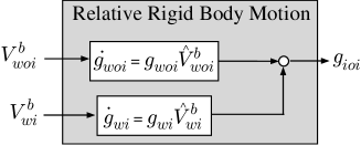
Figure 3: Block Diagram of Relative Rigid Body Motion

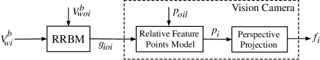
Figure 4: Block Diagram of the RRBM with Vision Camera (RRBM is an acronym for Relative Rigid Body Motion)

II-C Communication

The vision cameras have communication capability with the neighboring cameras and form a network. The communication is modeled by a digraph $G=({\mathcal{V}},{\mathcal{E}})$, where ${\mathcal{E}}\subset{\mathcal{V}}\times{\mathcal{V}}$ as in the left figure of Fig. 5. Namely, vision camera $i$ can get some information from $j$ if $(j,i)\in{\mathcal{E}}$. In addition, we define the neighbor set $\mathcal{N}_{i}$ of vision camera $i\in{\mathcal{V}}$ as

$$\mathcal{N}_{i}:=\{j\in{\mathcal{V}}|\ (j,i)\in{\mathcal{E}}\}.$$ (3)

Let us now employ the following assumption on the graph $G$.

Assumption 1

The communication graph $G$ is fixed, balanced and strongly connected.

The balanced and strongly connected graph is a graph such that there exists at least one directed path between any pair of nodes and the in-degree and out-degree are equal for all nodes [11].

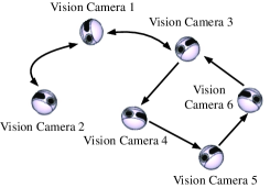
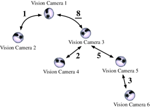
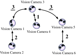
Figure 5: Left: Communication Graph, Middle: Tree with Root $1$ Minimizing $\tilde{D}$ ($\tilde{D}=8$), Right: Tree Minimizing ${D}$ ($W=3$)

We also denote by $G_{u}$ the undirected graph produced by replacing all the directed edges of $G$ by the undirected ones. Let ${\mathcal{T}}(i_{0})$ be the set of all spanning trees over $G_{u}$ with a root $i_{0}\in{\mathcal{V}}$ and we consider an element $G_{T}=({\mathcal{V}},{\mathcal{E}}_{T})\in{\mathcal{T}}(i_{0})$. Let the path from $i_{0}$ to a node $i\in{\mathcal{V}}$ along with the tree $G_{T}$ be denoted by $P_{G_{T}}(i)=(v_{0},\cdots,v_{d_{G_{T}}(i)}),\ v_{0}=i_{0},\ v_{d_{G_{T}}(i)}=i,\ (v_{l},v_{l+1})\in{\mathcal{E}}_{T}\ {\forall l}\in\{0,\cdots,d_{G_{T}}(i)-1\}$, where $d_{G_{T}}(i)$ denotes the length of the path $P_{G_{T}}(i)$. We also define

$$\delta_{G_{T}}(E;i)=\left\{\begin{array}[]{ll}1,&\mbox{if the path }P_{G_{T}}(i)\mbox{ includes edge }E\\ 0,&\mbox{otherwise}\end{array}\right.$$

for any $E\in{\mathcal{E}}_{T}$. By using the above notations, we define

$$W:=\min_{i_{0}\in{\mathcal{V}}}D(i_{0}),\ D(i_{0}):=\min_{G_{T}\in{\mathcal{T}}(i_{0})}\tilde{D}(G_{T}),\ \tilde{D}(G_{T}):=\max_{E\in{\mathcal{E}}_{T}}\sum_{i\in{\mathcal{V}}}\delta_{G_{T}}(E;i)d_{G_{T}}(i).$$ (4)

For example, let us consider the communication graph in Fig. 5(Left). Suppose that we choose $i_{0}=1$ and build a tree depicted in the middle figure of Fig. 5, where the number at around each edge is the value of $\sum_{i\in{\mathcal{V}}}\delta_{G_{T}}(E;i)d_{G_{T}}(i)$. Namely, $\tilde{D}$ is equal to $8$ for the tree and it is actually minimal for all spanning trees in ${\mathcal{T}}(1)$. However, choosing another node as a root can reduce the value of $\tilde{D}$. Indeed, as illustrated in the right figure of Fig. 5, a tree with $i_{0}=3$ achieves $\tilde{D}=3$, which is the minimal $D(i_{0})$ among all the choices of the root $i_{0}$.

II-D Average on $SO(3)$ and $SE(3)$

In this paper, the tuple of the relative rigid body motion (1), the visual measurement (2) and the communication structure (3) is called a visual sensor network. The objective of this paper is to present a cooperative estimation mechanism for the visual sensor networks meeting the following requirements simultaneously: Averaging for static objects, which means each camera $i$ estimates a pose close to an average of $\{g_{io_{j}}\}_{j\in{\mathcal{V}}},\ g_{io_{j}}:=g_{wi}^{-1}g_{wo_{j}}$, Tracking to moving objects, which means the estimates track the moving average pose within a bounded tracking error.

Let us now introduce the following mean $g^{*}$ on $SE(3)$ as an average of target poses $\{g_{wo_{j}}\}_{j\in{\mathcal{V}}}$.

$$g^{*}=(p^{*},{e^{\hat{\xi}\theta^{*}}}):=\arg\min_{g\in SE(3)}\sum_{j\in{\mathcal{V}}}\psi(g^{-1}g_{wo_{j}}),$$ (5)

where the function $\psi$ is defined for any $g=(p,{e^{\hat{\xi}\theta}})\in SE(3)$ as

$$\psi(g):=\frac{1}{2}\|I_{4}-g\|_{F}^{2}=\frac{1}{2}\|p\|^{2}+\phi({e^{\hat{\xi}\theta}}),\ \phi({e^{\hat{\xi}\theta}}):=\frac{1}{2}\|I_{3}-{e^{\hat{\xi}\theta}}\|_{F}^{2}={\rm tr}(I_{3}-{e^{\hat{\xi}\theta}})$$ (6)

and $\|M\|_{F}$ is the matrix Frobenius norm of matrix $M$. Hereafter, we also use the notation

$$g_{i}^{*}=(p_{i}^{*},{e^{\hat{\xi}\theta_{i}^{*}}}):=\arg\min_{g_{i}\in SE(3)}\sum_{j\in{\mathcal{V}}}\psi(g_{i}^{-1}g_{io_{j}})=g_{wi}^{-1}g^{*}.$$

The position average $p^{*}$ is equal to the arithmetic mean $p^{*}=\frac{1}{n}\sum_{j\in{\mathcal{V}}}p_{wo_{j}}$ of target positions $\{p_{wo_{j}}\}_{j\in{\mathcal{V}}}$ and the orientation average ${e^{\hat{\xi}\theta^{*}}}$ is a so-called Euclidean mean [25] of target orientations $\{{e^{\hat{\xi}\theta_{wo_{j}}}}\}_{j\in{\mathcal{V}}}$ defined by

$${e^{\hat{\xi}\theta^{*}}}:=\arg\min_{{e^{\hat{\xi}\theta}}\in SO(3)}\sum_{j\in{\mathcal{V}}}\phi({e^{-\hat{\xi}\theta}}{e^{\hat{\xi}\theta_{wo_{j}}}}).$$ (7)

It is known [25] that the Euclidean mean ${e^{\hat{\xi}\theta^{*}}}$ is given by

$${e^{\hat{\xi}\theta^{*}}}(t)={\rm Proj}\left(S(t)\right),\ S(t):=\frac{1}{n}\sum_{j\in{\mathcal{V}}}{e^{\hat{\xi}\theta_{wo_{j}}}}(t).$$ (8)

Here, ${\rm Proj}(M)$ is the orthogonal projection of $M\in{\cal{R}}^{3\times 3}$ onto $SO(3)$, which is given by $U_{M}V_{M}^{T}$ for the matrix $M$ with singular value decomposition $M=U_{M}\Sigma V_{M}^{T}$ [25].

Remark 1

Just computing the Euclidean mean is not so difficult even in a distributed fashion if we have prior knowledge that the target object is static. Indeed, the matrix $S$ is computed by using the consensus protocol under appropriate assumptions on the graph [10] and the operation ${\rm Proj}$ can be locally executed. However, such a scheme works only for static objects and never embodies tracking nature for moving target objects. The objective here is to present an estimation mechanism without using any prior knowledge and any decision-making process on whether the targets are static or moving.

III Networked Visual Motion Observer

III-A Visual Motion Observer

In this subsection, we consider the problem that vision camera $i$ estimates the target object motion $g_{io_{i}}$ from the visual measurements $f_{i}$ without considering communication. For the purpose, we introduce the visual motion observer presented in [8].

We first prepare a model of the rigid body motion (1) similarly to the Luenberger observer as

$$\dot{\bar{g}}_{io_{i}}=-\hat{V}_{wi}^{b}\bar{g}_{io_{i}}+\bar{g}_{io_{i}}\hat{u}_{ei},$$ (9)

where $\bar{g}_{io_{i}}=(\bar{p}_{io_{i}},e^{\hat{\bar{\xi}}\bar{\theta}_{io_{i}}})$ is the estimate of the actual relative pose $g_{io_{i}}$. The input $u_{ei}=(v_{uei},\ \omega_{uei})$ is to be determined to drive the estimated value $\bar{g}_{io_{i}}$ to the actual $g_{io_{i}}$.

In order to establish the estimation error system, we define the estimation error between the estimated value $\bar{g}_{io_{i}}$ and the actual relative rigid body motion $g_{io_{i}}$ as $g_{ei}=(p_{ei},e^{\hat{\xi}\theta_{ei}}):=\bar{g}_{io_{i}}^{-1}g_{io_{i}}$. Using the notations $e_{R}(e^{\hat{\xi}\theta}):={\rm sk}(e^{\hat{\xi}\theta})^{\vee}$ and ${\rm sk}(e^{\hat{\xi}\theta}):=\frac{1}{2}(e^{\hat{\xi}\theta}-e^{-\hat{\xi}\theta})$, the vector representation of the estimation error $g_{ei}$ is given by

$$e_{ei}:=E_{R}(g_{ei}),\ E_{R}(g_{ei}):=\left[\begin{array}[]{cc}p_{ei}^{T}&e_{R}^{T}(e^{\hat{\xi}\theta_{ei}})\end{array}\right]^{T}.$$ (11)

Once the estimate $\bar{g}_{io_{i}}$ is determined, the estimated measurement $\bar{f}_{i}$ is also computed by (2). Let us now define the visual measurement error as $f_{ei}:=f_{i}(g_{io_{i}})-\bar{f}_{i}(\bar{g}_{io_{i}})$. Then, the measurement error vector $f_{ei}$ can be approximately given by $f_{ei}=J_{i}(\bar{g}_{io_{i}})e_{ei}$ [8], where $J_{i}(\bar{g}_{io_{i}}):SE(3)\rightarrow{\cal{R}}^{2m\times 6}$ is the well-known image Jacobian. Now, if $m\geq 4$, the image Jacobian has the full column rank and the estimation error vector $e_{ei}$ is reconstructed as

$$e_{ei}=J_{i}^{\dagger}(\bar{g}_{io_{i}})f_{ei},$$ (12)

where $\dagger$ denotes the pseudo-inverse.

Differentiating $g_{ei}=\bar{g}_{io_{i}}^{-1}g_{io_{i}}$ with respect to time and using (1) and (9), we obtain the estimation error system

$$\dot{g}_{ei}=-\hat{u}_{ei}g_{ei}+g_{ei}\hat{V}_{wo_{i}}^{b}.$$ (13)

Fig. 7 shows the block diagram of the system (13).

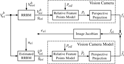
Figure 6: Estimation Error System

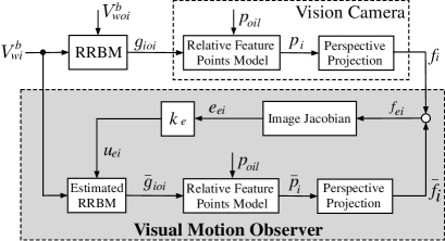
Figure 7: Visual Motion Observer

The paper [8] proves that if $V_{wo_{i}}^{b}=0$, then the estimation error system (13) is passive from the input $u_{ei}$ to the output $-e_{ei}$.

Based on passivity-based control theory, we close the loop by using the input

$$u_{ei}=-k_{e}(-e_{ei})=k_{e}e_{ei},\ k_{e}>0.$$ (14)

Then, the resulting total estimation mechanism formulated as

$$\mbox{Visual Motion Observer: }\left\{\begin{array}[]{lr}\dot{\bar{g}}_{io_{i}}=-\hat{V}_{wi}^{b}\bar{g}_{io_{i}}+\bar{g}_{io_{i}}\hat{u}_{ei}&\cdots(\ref{eqn:EsRRBM})\\ e_{ei}=J_{i}^{\dagger}(\bar{g}_{io_{i}})f_{ei}&\cdots(\ref{eqn:e_e})\\ u_{ei}=k_{e}e_{ei}&\cdots(\ref{eqn:vmo_input})\end{array}\right.$$ (18)

is called visual motion observer [9], whose block diagram is illustrated in Fig. 7. In terms of the mechanism, we immediately obtain the following facts from passivity.

Fact 1

[8] (i) If $V_{wo_{i}}^{b}=0$, then the equilibrium point $e_{ei}=0$ for the closed-loop system (13) with (14) is asymptotically stable. (ii) Given a positive scalar $\nu_{i}$, if $k_{e}$ satisfies $k_{e}-\frac{1}{2\nu_{i}^{2}}-\frac{1}{2}>0$, then the system (13) and (14) with input $V^{b}_{wo_{i}}$ and output $e_{ei}$ has $L_{2}$-gain smaller than $\nu_{i}$.

Item (i) means the visual motion observer leads the estimate $\bar{g}_{io_{i}}$ to the actual $g_{io_{i}}$ for a static object. Item (ii) implies that the observer also works for a moving target object, and the parameter $\nu_{i}$ is an index on estimation accuracy when the observer is applied to a moving target.

III-B Networked Visual Motion Observer

The objective of this paper is to achieve averaging, while preserving the tracking nature of the visual motion observer. For this purpose, this subsection presents a cooperative estimation mechanism under the assumption of (i) each vision camera knows relative pose $g_{ij}=g_{wi}^{-1}g_{wj}$ with respect to neighbors $j\in\mathcal{N}_{i}$ and (ii) all the vision cameras are static, i.e. $V^{b}_{wi}=0\ {\forall i}\in{\mathcal{V}}$.

Under $V^{b}_{wi}=0$, the relative rigid body motion (1) is simply given by $\dot{g}_{io_{i}}=g_{io_{i}}\hat{V}_{wo_{i}}^{b}$. Accordingly, the update procedure in (18) is reformulated as

$$\dot{\bar{g}}_{io_{i}}=\bar{g}_{io_{i}}\hat{u}_{ei},\ u_{ei}=k_{e}e_{ei}.$$ (19)

Then, the following proposition holds in terms of the procedure (19).

Proposition 1

[31] The update procedure (19) is a gradient decent algorithm on $SE(3)$ for the potential function $\psi(\bar{g}_{io_{i}}g_{io_{i}})$, where the function $\psi$ is defined in (6).

Let us now view $\psi(\bar{g}^{-1}_{io_{i}}g_{io_{i}})=\psi(\bar{g}^{-1}_{wo_{i}}g_{wo_{i}})$ as the local objective function to be minimized by vision camera $i$. Then, we see that the group objective (5) is given by the sum of the local objective functions for all $i\in{\mathcal{V}}$. Note that each vision camera does not know the local objective of the other vision cameras. Under such a situation computing a solution minimizing the global objective function by using local negotiations is called multi-agent optimization problem and [32] presents an update rule of the local estimates of the solution to produce approximate solutions to the global objective combining the gradient decent algorithm of the local objective function and the consensus protocol [10]. The present cooperative estimation mechanism is inspired by the algorithm but the consensus protocol cannot be executed on $SE(3)$. We thus instead use a pose synchronization law presented in [15], which is also based on passivity of rigid body motion.

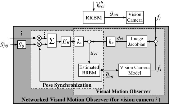
Figure 8: Networked Visual Motion Observer

We next present an update rule of the estimates $\bar{g}_{io_{i}}$ so as to estimate the average $g_{i}^{*}$. Each vision camera $i$ first gains the estimates $\bar{g}_{jo_{j}}$ from $j\in\mathcal{N}_{i}$ as messages. Now, by multiplying known information $g_{ij}$ from left, each vision camera $i$ gets $\bar{g}_{io_{j}}:=g_{ij}\bar{g}_{jo_{j}}$ for all $j\in\mathcal{N}_{i}$. Using the information, the estimate $\bar{g}_{io_{i}}$ is updated according to (9) with

$${u}_{ei}=k_{e}e_{ei}+k_{s}\sum_{j\in\mathcal{N}_{i}}E_{R}(\bar{g}_{io_{i}}^{-1}\bar{g}_{io_{j}}),\ k_{e}>0,\ k_{s}>0.$$ (20)

Since $e_{ei}$ is reconstructed from the visual measurement $f_{i}$ by (12) and $\bar{g}_{io_{j}}$ is obtained through communication as stated above, the update procedure (20) is implementable.

The present input (20) consists of the visual feedback term $k_{e}e_{ei}$ and the mutual feedback term $k_{s}\sum_{j\in\mathcal{N}_{i}}E_{R}(\bar{g}_{io_{i}}^{-1}\bar{g}_{io_{j}})$, where the former is inspired by the visual motion observer [8] and the latter is by the pose synchronization law [15]. Indeed, without the second term, the update rule (20) is the same as that of the visual motion observer (19). In addition, without the visual feedback, the update procedure (20), namely ${u}_{ei}=k_{s}\sum_{j\in\mathcal{N}_{i}}E_{R}(\bar{g}_{io_{i}}^{-1}\bar{g}_{io_{j}})$, is essentially equivalent to the passivity-based pose synchronization law [15] of a group of rigid bodies with states $\bar{g}_{wo_{i}}:=g_{wi}\bar{g}_{io_{i}}$. Thus, under appropriate assumptions, each state $\bar{g}_{wo_{i}}$ would converge to a state satisfying $\bar{g}_{wo_{i}}=\bar{g}_{wo_{j}}\ {\forall i,j}\in{\mathcal{V}}$ as time goes to infinity without the visual feedback term.

In other words, the visual motion observers are networked by the mutual feedback term in the total estimation mechanism formulated as

$$\mbox{ Networked VMO: }\left\{\begin{array}[]{ll}\dot{\bar{g}}_{io_{i}}=\bar{g}_{io_{i}}\hat{u}_{ei}&\cdots(\ref{eqn:EsRRBM})\\ e_{ei}=J_{i}^{\dagger}(\bar{g}_{io_{i}})f_{ei}&\cdots(\ref{eqn:e_e})\\ {u}_{ei}=k_{e}e_{ei}+k_{s}\sum_{j\in\mathcal{N}_{i}}E_{R}(\bar{g}_{io_{i}}^{-1}\bar{g}_{io_{j}})&\cdots(\ref{eqn:ce_update})\end{array}\right.{\forall i}\in{\mathcal{V}},$$ (24)

where VMO is an acronym for Visual Motion Observer. This is why the estimation mechanism is called networked visual motion observer. The block diagram of the total system of vision camera $i$ is illustrated in Fig. 8.

IV Averaging Performance Analysis

In this section, we derive ultimate estimation accuracy of the average $g_{i}^{*}$ achieved by the networked visual motion observer (24) under the following assumption.

Assumption 2

(i) The target objects are static, i.e. $V^{b}_{wo_{i}}=0\ {\forall i}\in{\mathcal{V}}$.
(ii) There exists a pair $(i,j)\in{\mathcal{V}}\times{\mathcal{V}}$ such that $p_{wo_{i}}\neq p_{wo_{j}}$ and ${e^{\hat{\xi}\theta_{wo_{i}}}}\neq{e^{\hat{\xi}\theta_{wo_{j}}}}$.
(iii) ${e^{-\hat{\xi}\theta_{i}^{*}}}{e^{\hat{\xi}\theta_{io_{i}}}}>0$ for all $i\in{\mathcal{V}}$.

The moving target objects will be investigated in Section V. The item (ii) is assumed in order to avoid a meaningless problem such that $g_{wo_{i}}=g_{wo_{j}}\ {\forall i,j}\in{\mathcal{V}}$. Indeed, under the situation, it is straightforward to prove convergence of the estimates to the common pose. In terms of the item (iii), we see that if ${e^{-\hat{\xi}\theta_{wo_{i}}}}{e^{\hat{\xi}\theta_{wo_{j}}}}>0$ for all $i,j\in{\mathcal{V}}$, then the following inequality holds.

$$\phi({e^{-\hat{\xi}\theta_{i}^{*}}}{e^{\hat{\xi}\theta_{io_{i}}}})\leq\phi_{m}:=\max_{i,j\in{\mathcal{V}}}\phi({e^{-\hat{\xi}\theta_{wo_{i}}}}{e^{\hat{\xi}\theta_{wo_{j}}}})\ {\forall i}\in{\mathcal{V}}$$ (25)

Inequality (25) implies that if ${e^{-\hat{\xi}\theta_{wo_{i}}}}{e^{\hat{\xi}\theta_{wo_{j}}}}>0\ {\forall i,j}\in{\mathcal{V}}$ ($\phi_{m}$ is smaller than $2$), then (iii) is satisfied. Thus, (iii) can be checked if set-valued prior information on the target orientations, i.e. an upper bound of $\phi_{m}$ is available.

IV-A Definition of Averaging Performance

In this subsection, we introduce a notion of approximate averaging. For this purpose, we define the following sets for any positive parameter $\varepsilon$.

$$\Omega_{p}(\varepsilon):=\left\{(\bar{p}_{io_{i}})_{i\in{\mathcal{V}}}\left|\ \frac{1}{2}\sum_{i\in{\mathcal{V}}}\|\bar{p}_{io_{i}}-p^{*}_{i}\|^{2}\leq\varepsilon\rho_{p}\right.\right\},\ \rho_{p}:=\frac{1}{2}\sum_{i\in{\mathcal{V}}}\|{p}_{io_{i}}-p^{*}_{i}\|^{2}$$ (26)

$$\Omega_{R}(\varepsilon):=\left\{({e^{\hat{\bar{\xi}}\bar{\theta}_{io_{i}}}})_{i\in{\mathcal{V}}}\left|\ \sum_{i\in{\mathcal{V}}}\phi({e^{-\hat{\xi}\theta_{i}^{*}}}{e^{\hat{\bar{\xi}}\bar{\theta}_{io_{i}}}})\leq\varepsilon\rho_{R}\right.\right\},\ \rho_{R}:=\sum_{i\in{\mathcal{V}}}\phi({e^{-\hat{\xi}\theta_{i}^{*}}}{e^{\hat{\xi}\theta_{io_{i}}}})$$ (27)

Let us now define $\varepsilon$-level averaging performance to be met by the estimates $\bar{g}_{io_{i}}=(\bar{p}_{io_{i}},{e^{\hat{\bar{\xi}}\bar{\theta}_{io_{i}}}})$.

Definition 1

Given target poses $(g_{io_{i}})_{i\in{\mathcal{V}}}$, position estimates $(\bar{p}_{io_{i}})_{i\in{\mathcal{V}}}$ are said to achieve $\varepsilon$-level averaging performance for a scalar $\varepsilon>0$ if there exists a finite $T$ such that $(\bar{p}_{io_{i}}(t))_{i\in{\mathcal{V}}}\in\Omega_{p}(\varepsilon)\ {\forall t}\geq T$ and the orientation estimates $({e^{\hat{\bar{\xi}}\bar{\theta}_{io_{i}}}})_{i\in{\mathcal{V}}}$ are said to achieve $\varepsilon$-level averaging performance if there exists a finite $T$ such that $({e^{\hat{\bar{\xi}}\bar{\theta}_{io_{i}}}}(t))_{i\in{\mathcal{V}}}\in\Omega_{R}(\varepsilon)\ {\forall t}\geq T$.

In the absence of communication, each vision camera $i$ acquires no information on the target objects $o_{j},\ j\neq i$. Under the situation, what each vision camera can do is to produce as an accurate estimate of the relative pose $g_{io_{i}}$ as possible. Namely, the parameters $\rho_{p}$ and $\rho_{R}$ specify the best performance of average estimation in the absence of communication. More specifically, since the visual motion observer (18) correctly estimates the static target object pose $g_{io_{i}}$ (Fact 1), the parameters $\rho_{p}$ and $\rho_{R}$ indicate the average estimation accuracy in the absence of the mutual feedback term of $u_{ei}$ in (20). Namely, the parameter $\varepsilon$ is an indicator of improvement of average estimation accuracy by inserting the mutual feedback term $k_{s}\sum_{j\in\mathcal{N}_{i}}E_{R}(\bar{g}_{io_{i}}^{-1}\bar{g}_{io_{j}})$.

IV-B Auxiliary Results

In this subsection, we give some results necessary for proving the main result of this section.

Lemma 1

Suppose that the estimates $(\bar{g}_{io_{i}})_{i\in{\mathcal{V}}}$ are updated by the networked visual motion observer (24). Then, under Assumptions 1 and 2 and ${e^{-\hat{\bar{\xi}}\bar{\theta}_{io_{i}}}}{e^{\hat{\xi}\theta_{i}^{*}}}>0\ {\forall t}\geq 0$, for all $c>0$, there exists a finite $\tau(c)$ such that $\phi({e^{-\hat{\xi}\theta_{i}^{*}}}{e^{\hat{\bar{\xi}}\bar{\theta}_{io_{i}}}})\leq\phi({e^{-\hat{\xi}\theta^{*}}}{e^{\hat{\xi}\theta_{wo_{h}}}})+c\ {\forall t}\geq\tau(c),\ i\in{\mathcal{V}}$, where $h:=\arg\max_{j\in{\mathcal{V}}}\phi({e^{-\hat{\xi}\theta^{*}}}{e^{\hat{\xi}\theta_{wo_{j}}}})$.

Proof:

See Appendix A. ∎

Lemma 1 implies that the individual estimate ${e^{\hat{\bar{\xi}}\bar{\theta}_{io_{i}}}}$ gets closer to the average ${e^{\hat{\xi}\theta_{i}^{*}}}$ at least than the object with the farthest orientation from the average. In addition, the proof of this lemma also means that the set

$${\mathcal{S}}=\{({e^{\hat{\bar{\xi}}\bar{\theta}_{io_{i}}}})_{i\in{\mathcal{V}}}|\ {e^{-\hat{\bar{\xi}}\bar{\theta}_{io_{i}}}}{e^{\hat{\xi}\theta_{i}^{*}}}>0\ {\forall i}\in{\mathcal{V}}\}$$

is positively invariant for the total system (24) under Assumption 2. Namely, if ${e^{-\hat{\bar{\xi}}\bar{\theta}_{io_{i}}}}{e^{\hat{\xi}\theta_{i}^{*}}}>0$ is satisfied at the initial time, then ${e^{-\hat{\bar{\xi}}\bar{\theta}_{io_{i}}}}{e^{\hat{\xi}\theta_{i}^{*}}}>0$ holds for all subsequent time.

We next have the following lemma.

Lemma 2

Suppose that the estimates $(\bar{g}_{io_{i}})_{i\in{\mathcal{V}}}$ are updated by the networked visual motion observer (24). Then, under Assumptions 1 and 2, if the initial estimates satisfy $({e^{\hat{\bar{\xi}}\bar{\theta}_{io_{i}}}}(0))_{i\in{\mathcal{V}}}\in{\mathcal{S}}$, both of the estimates $(\bar{p}_{io_{i}})_{i\in{\mathcal{V}}}$ and $({e^{\hat{\bar{\xi}}\bar{\theta}_{io_{i}}}})_{i\in{\mathcal{V}}}$ achieve $1$-level averaging performance.

Proof:

See Appendix B. ∎

This lemma is proved by using the energy functions

$$\ \ U_{p}:=\frac{1}{2}\sum_{i\in{\mathcal{V}}}\|p_{i}^{*}-\bar{p}_{io_{i}}\|^{2}=\frac{1}{2}\sum_{i\in{\mathcal{V}}}\|p^{*}-\bar{p}_{wo_{i}}\|^{2},\ {U}_{R}:=\sum_{i\in{\mathcal{V}}}\phi({e^{-\hat{\xi}\theta_{i}^{*}}}{e^{\hat{\bar{\xi}}\bar{\theta}_{io_{i}}}})=\sum_{i\in{\mathcal{V}}}\phi({e^{-\hat{\xi}\theta^{*}}}{e^{\hat{\bar{\xi}}\bar{\theta}_{wo_{i}}}})$$

which are defined by the sum of individual error between the average and the estimate. The functions $U_{p}\geq 0$ and $U_{R}\geq 0$ are equal to $0$ if and only if $\bar{p}_{io_{i}}=p_{i}^{*}$ and ${e^{\hat{\bar{\xi}}\bar{\theta}_{io_{i}}}}={e^{\hat{\xi}\theta_{i}^{*}}}\ {\forall i}\in{\mathcal{V}}$ respectively. The selection of the energy function is inspired by one of our previous works on pose synchronization [15] whose framework is originally presented in [13].

Lemma 2 means that the average estimation as a group in the presence of communication is at least more accurate than the case in the absence of communication. However, this lemma does not say how accurate estimates of the average the networked visual motion observer produces.

From Lemmas 1 and 2, the estimates $(\bar{p}_{io_{i}})_{i\in{\mathcal{V}}}$ and $({e^{\hat{\bar{\xi}}\bar{\theta}_{io_{i}}}})_{i\in{\mathcal{V}}}$ settle into $\Omega_{p}(1)$ and ${\mathcal{S}}^{R}_{1}:={\mathcal{S}}\cap\Omega_{R}(1)$ in finite time, respectively. Let us now define the following subsets of $\Omega_{p}(1)$ and ${\mathcal{S}}^{R}_{1}$.

$${\mathcal{S}}^{p}_{2}(k):=\Big{\{}(\bar{p}_{io_{i}})_{i\in{\mathcal{V}}}\in\Omega_{p}(1)\Big{|}\sum_{i\in{\mathcal{V}}}\sum_{j\in\mathcal{N}_{i}}\frac{1}{2}\|\bar{p}_{wo_{i}}-\bar{p}_{wo_{j}}\|^{2}\geq k\rho_{p}\Big{\}},\$$

$${\mathcal{S}}^{R}_{2}(k):=\Big{\{}({e^{\hat{\bar{\xi}}\bar{\theta}_{io_{i}}}})_{i\in{\mathcal{V}}}\in{\mathcal{S}}^{R}_{1}\Big{|}\beta\sum_{i\in{\mathcal{V}}}\sum_{j\in\mathcal{N}_{i}}\phi({e^{-\hat{\bar{\xi}}\bar{\theta}_{wo_{i}}}}{e^{\hat{\bar{\xi}}\bar{\theta}_{wo_{j}}}})\geq k\rho_{R}\Big{\}},\$$

$${\mathcal{S}}^{p}_{3}(k,\varepsilon):=\Omega_{p}(1)\setminus({\mathcal{S}}^{p}_{2}(k)\cup\Omega_{p}(\varepsilon)),\ {\mathcal{S}}^{R}_{3}(k,\varepsilon):={\mathcal{S}}^{R}_{1}\setminus({\mathcal{S}}^{R}_{2}(k)\cup\Omega_{R}(\varepsilon))$$

for some $\varepsilon\in[0,1)$, where $\beta:=1-\sqrt{2(\phi({e^{-\hat{\xi}\theta^{*}}}{e^{\hat{\xi}\theta_{wo_{h}}}})+c)}$ and $k=k_{e}/k_{s}$. Images of the subsets on the position space are depicted in Fig. 9. We see from the figure that

$$\Omega_{p}(1)\setminus({\mathcal{S}}^{p}_{2}(k)\cup{\mathcal{S}}^{p}_{3}(k,\varepsilon))\subseteq\Omega_{p}(\varepsilon),\ {\mathcal{S}}^{R}_{1}\setminus({\mathcal{S}}^{R}_{2}(k)\cup{\mathcal{S}}^{R}_{3}(k,\varepsilon))\subseteq\Omega_{R}(\varepsilon).$$ (28)

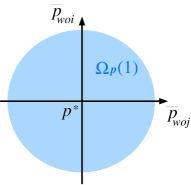
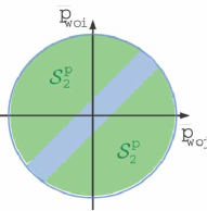
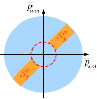
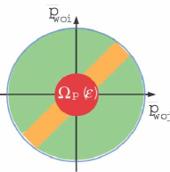
Figure 9: Images of Each Subsets (Position)

In terms of the subsets ${\mathcal{S}}^{p}_{2}(k)$ and ${\mathcal{S}}^{R}_{2}(k)$, we have the following lemma.

Lemma 3

Suppose that all the assumptions in Lemma 2 hold and $\beta>0$. Then, the time derivative of $U_{p}$ and $U_{R}$ along with the trajectories of (24) are strictly negative as long as $(\bar{p}_{io_{i}})_{i\in{\mathcal{V}}}\in{\mathcal{S}}^{p}_{2}(k)$ and $({e^{\hat{\bar{\xi}}\bar{\theta}_{io_{i}}}})_{i\in{\mathcal{V}}}\in{\mathcal{S}}^{R}_{2}(k)$ respectively, at least after the time $\tau(c)$.

Proof:

See Appendix C. ∎

From (25), $\beta$ can be estimated by set-valued prior information on the target orientations i.e. $\phi_{m}$.

IV-C Averaging Performance

We are now ready to state the main result of this section on averaging accuracy attained by the networked visual motion observer (24).

Theorem 1

Suppose that all the assumptions in Lemma 2 hold. Then, for any $\epsilon\in(0,1)$, position estimates $(\bar{p}_{io_{i}})_{i\in{\mathcal{V}}}$ achieve $\varepsilon_{p}$-level averaging performance with

$$\varepsilon_{p}=\left\{\begin{array}[]{ll}1-(1-\epsilon)\left(1-\sqrt{kW}\right)^{2}&\mbox{if }k\leq 1/W\\ 1&\mbox{otherwise}\end{array}\right.,$$ (31)

and orientation estimates $({e^{\hat{\bar{\xi}}\bar{\theta}_{io_{i}}}})_{i\in{\mathcal{V}}}$ achieve $\varepsilon_{R}$-level averaging performance with

$$\varepsilon_{R}=\left\{\begin{array}[]{ll}1-(1-\epsilon)\left(\sqrt{\beta}-\sqrt{kW}\right)^{2},&\mbox{if }k\leq\beta/W,\ \beta>0\\ 1,&\mbox{otherwise}\end{array}\right.,$$ (34)

where $W$ is defined in (4).

Proof:

See Appendix D. ∎

Suppose that $\epsilon$ is taken sufficiently close to $0$. Then, we see that both of the parameters $\varepsilon_{p}$ and $\varepsilon_{R}$ become small as the term $\sqrt{kW}$ approaches to $0$. Note that if we use a sufficiently small $k$ ($k_{s}\gg k_{e}$) in (20), the term is approximated by $0$. Here, we see an essential difference between the position and orientation estimates. The definition of $\varepsilon_{p}$ with $\epsilon\approx 1$ indicates that we can get arbitrarily accurate estimation of the average $p_{i}^{*}$ by choosing a sufficiently small $k$. In contrast, we see from the definition of $\varepsilon_{R}$ that an offset associated with $\sqrt{\beta}(<1)$ occurs for the orientation estimates regardless of the parameter $k$. From the definition of $\beta:=1-\sqrt{2(\phi({e^{-\hat{\xi}\theta^{*}}}{e^{\hat{\xi}\theta_{wo_{h}}}})+c)}$, if the target object’s orientation ${e^{\hat{\xi}\theta_{wo_{h}}}}$ is sufficiently close to the average ${e^{-\hat{\xi}\theta^{*}}}$, i.e. if ${e^{\hat{\xi}\theta_{wo_{i}}}}$ and ${e^{\hat{\xi}\theta_{wo_{j}}}}$ are close among all $i,j\in{\mathcal{V}}$ enough to approximate all the orientations by matrices on a tangent vector space of $SO(3)$ at ${e^{\hat{\xi}\theta_{wo_{i}}}}$, then it becomes close to $0$ and the average is accurately estimated by the networked visual motion observer (24). Otherwise, the accuracy might degrade, though it is more accurate at least than the case in the absence of communication.

V Tracking Performance Analysis

In this section, we analyze the tracking performance of the estimates $\{\bar{g}_{io_{i}}\}_{i\in{\mathcal{V}}}$ to the average $g_{i}^{*}$ for moving targets when the networked visual motion observer is applied to the visual sensor networks under the following assumption.

Assumption 3

(i) The target body velocities $V^{b}_{wo_{i}}(t),\ i\in{\mathcal{V}}$ are continuous in $t$ and bounded as

$$\|v^{b}_{wo_{i}}(t)\|_{2}^{2}\leq\bar{w}_{p}^{2},\ \|\omega^{b}_{wo_{i}}(t)\|^{2}\leq\bar{w}_{R}^{2}\ {\forall i\in{\mathcal{V}}},\ t\geq 0.$$ (35)

(ii) For all $t\geq 0$, there exists $(i(t),j(t))\in{\mathcal{V}}\times{\mathcal{V}}$ such that $p_{wo_{i(t)}}\neq p_{wo_{j(t)}}$ and $e^{\hat{\xi}\theta_{wo_{i(t)}}}\neq e^{\hat{\xi}\theta_{wo_{j(t)}}}$.
(iii) ${e^{-\hat{\xi}\theta_{wo_{j}}}}(t){e^{\hat{\xi}\theta_{wo_{i}}}}(t)>0$ for all $i,j\in{\mathcal{V}}$ and $t\geq 0$.

V-A Description of Average Motion

In this subsection, we first formulate the motion of the average $g^{*}=(p^{*},{e^{\hat{\xi}\theta^{*}}})$. The behavior of the position average $p^{*}$ is clearly described by

$$\dot{p}^{*}={e^{\hat{\xi}\theta^{*}}}v^{b,*},\ v^{b,*}:={e^{-\hat{\xi}\theta^{*}}}\left(\frac{1}{n}\sum_{i\in{\mathcal{V}}}{e^{\hat{\xi}\theta_{wo_{i}}}}v^{b}_{woi}\right)$$ (36)

from the definition of $p^{*}=\frac{1}{n}\sum_{i\in{\mathcal{V}}}p_{wo_{i}}$. Meanwhile, the trajectory of the orientation average ${e^{\hat{\xi}\theta^{*}}}$ described by (8) satisfies the following lemma.

Lemma 4

Under Assumption 3, the average ${e^{\hat{\xi}\theta^{*}}}$ is continuously differentiable.

Proof:

From the polar decomposition, we get $S(t)={e^{\hat{\xi}\theta^{*}}}(t)P_{S}(t)$ [25], where $S(t)=\frac{1}{n}\sum_{i\in{\mathcal{V}}}{e^{\hat{\xi}\theta_{wo_{i}}}}$ and $P_{S}^{2}(t)=S^{T}(t)S(t)$. Under Assumption 3(iii), we have ${e^{-\hat{\xi}\theta_{wo_{j}}}}(t)S(t)>0$ and hence $P_{S}(t)$ is invertible for all ${t}\geq 0$. Thus, the average ${e^{\hat{\xi}\theta^{*}}}$ is given by ${e^{\hat{\xi}\theta^{*}}}(t)=S(t)P_{S}^{-1}(t)$. From (1), the matrices $S(t)$ and $P_{S}(t)$ are clearly differentiable from their definitions and hence ${\dot{e}^{\hat{\xi}\theta^{*}}}$ is well defined. Moreover, from Assumption 3(i), both of $\dot{S}(t)$ and $\dot{P}_{S}(t)$ are continuous and $\frac{d}{dt}(P_{S}^{-1})=P_{S}^{-1}(t)\dot{P}_{S}P_{S}^{-1}$ is also continuous, which implies that ${\dot{e}^{\hat{\xi}\theta^{*}}}(t)$ is also continuous. Hence, the average ${e^{\hat{\xi}\theta^{*}}}$ is continuously differentiable. This completes the proof. ∎

Moreover, since ${e^{\hat{\xi}\theta^{*}}}(t)\in SO(3)$ holds for all $t\geq 0$, the derivative ${{\dot{e}^{\hat{\xi}\theta^{*}}}}$ has to satisfy ${\dot{e}^{\hat{\xi}\theta^{*}}}\in T_{{e^{\hat{\xi}\theta^{*}}}}SO(3)$, where $T_{{e^{\hat{\xi}\theta^{*}}}}SO(3):=\{{e^{\hat{\xi}\theta^{*}}}X|\ X\in so(3)\}$ is the tangent space of the manifold $SO(3)$ at ${e^{\hat{\xi}\theta^{*}}}$. Namely, the trajectory of the Euclidean mean ${e^{\hat{\xi}\theta^{*}}}$ is described by the differential equation ${\dot{e}^{\hat{\xi}\theta^{*}}}={e^{\hat{\xi}\theta^{*}}}\hat{\omega}^{b,*}$ with some body velocity $\hat{\omega}^{b,*}\in so(3)$.

We next clarify a relation between velocities $V^{b,*}:=(v^{b,*},\omega^{b,*})$ and $V^{b}_{wo_{i}}=(v^{b}_{wo_{i}},\omega^{b}_{wo_{i}}),\ {i\in{\mathcal{V}}}$. We first define $w_{p}:=(v^{b}_{wo_{i}})_{i\in{\mathcal{V}}}$ and $w_{R}:=(\omega^{b}_{wo_{i}})_{i\in{\mathcal{V}}}$. Since it is easy from (36) to obtain $\|v^{b,*}\|^{2}\leq\|w_{p}\|^{2}/n$, we mention only a relation between $\omega^{b,*}$ and $w_{R}$ in the following.

Lemma 5

Suppose that the target orientations $({e^{\hat{\xi}\theta_{wo_{i}}}})_{i\in{\mathcal{V}}}$ satisfy

$$\left\|{e^{\hat{\xi}\theta^{*}}}(t)-S(t)\right\|_{F}\leq\gamma\ {\forall t}\geq 0$$ (37)

for some $\gamma>0$. Then, the following inequality holds.

$$\|\omega^{b,*}(t)\|^{2}<\frac{\mu^{2}(\gamma)}{n}\|w_{R}(t)\|^{2},\ \mu(\gamma):=\frac{\sqrt{2}}{\sqrt{2}-\gamma}$$ (38)

Proof:

See Appendix E ∎

Though we omit the proof, $\left\|{e^{\hat{\xi}\theta^{*}}}(t)-S(t)\right\|_{F}$ is also upper bounded by $\phi_{m}$ and hence $\gamma$ is estimated by prior information on the target orientations.

V-B Tracking Performance

Let us consider the whole networked system $\Sigma_{track}$ consisting of the relative rigid body motion (1) for all $i\in{\mathcal{V}}$ and the networked visual motion observer (24). Here, we regard the collections of body velocities of the target objects $(V^{b}_{wo_{i}})_{i\in{\mathcal{V}}}$, i.e. $w=(w_{p},w_{R})$, as the external disturbance to $\Sigma_{track}$ and evaluate the error between the estimates $(\bar{g}_{io_{i}})_{i\in{\mathcal{V}}}$ and the average $g^{*}_{i}$ in the presence of the disturbance $w$. Namely, we let the error $(\{g_{i}^{*}\}^{-1}\bar{g}_{io_{i}})_{i\in{\mathcal{V}}}$ be the output signal of $\Sigma_{track}$.

Unlike the static objects case, $\rho_{p}=\frac{1}{2}\sum_{i\in{\mathcal{V}}}\|p_{io_{i}}-p^{*}_{i}\|^{2}$ and $\rho_{R}=\sum_{i\in{\mathcal{V}}}\phi({e^{-\hat{\xi}\theta_{i}^{*}}}{e^{\hat{\xi}\theta_{io_{i}}}})$ are also time-varying. We thus define the parameters

$$\rho^{\prime}_{p}:=\sup_{t}\rho_{p}(t),\ \rho^{\prime}_{R}:=\sup_{t}\rho_{R}(t)$$

assuming $\rho_{p}^{\prime}<\infty$ and redefine the sets $\Omega_{p}^{\prime}$ and $\Omega_{R}^{\prime}$ by just replacing $\rho_{p}$ and $\rho_{R}$ in (26) and (27) by $\rho_{p}^{\prime}$ and $\rho_{R}^{\prime}$, respectively. The parameters $\rho^{\prime}_{p}$ and $\rho^{\prime}_{R}$ are the suprimum of the distance from the estimate to the average when $g_{io_{i}}$ is correctly estimated and hence they are also indicators of the best average estimation performance in the absence of communication. Note however that the visual motion observer (18) cannot correctly estimate $g_{io_{i}}$ as long as the object is moving with unknown velocity.

The problem to be considered here is redefined as follows.

Definition 2

The position estimates $(\bar{p}_{io_{i}})_{i\in{\mathcal{V}}}$ are said to achieve $\varepsilon$-level tracking performance for a positive scalar $\varepsilon$ if there exists a finite $T$ such that $(\bar{p}_{io_{i}}(t))_{i\in{\mathcal{V}}}\in\Omega_{p}^{\prime}(\varepsilon)\ {\forall w}\in{\mathcal{W}}\mbox{ and }t\geq T$, where ${\mathcal{W}}$ is the set of the disturbance signal $w(\cdot)$ satisfying Assumption 3. Similarly, the estimates $({e^{\hat{\bar{\xi}}\bar{\theta}_{io_{i}}}})_{i\in{\mathcal{V}}}$ are said to achieve $\varepsilon$-level tracking performance if there exists a finite $T$ such that $({e^{\hat{\bar{\xi}}\bar{\theta}_{io_{i}}}}(t))_{i\in{\mathcal{V}}}\in\Omega_{R}^{\prime}(\varepsilon)\ {\forall w}\in{\mathcal{W}}\mbox{ and }{t}\geq T$.

In terms of the tracking performance defined above, we have the following theorem.

Theorem 2

Suppose that the estimates $\bar{g}_{io_{i}}$ are updated according to (24). Under Assumptions 1 and 3, if $k_{e}>\mu^{2}(\gamma)$ for $\gamma$ satisfying (37) and $({e^{\hat{\bar{\xi}}\bar{\theta}_{io_{i}}}}(t))_{i\in{\mathcal{V}}}\in{\mathcal{S}}\ {\forall t}\geq 0$, the estimates $(\bar{p}_{io_{i}})_{i\in{\mathcal{V}}}$ and $({e^{\hat{\bar{\xi}}\bar{\theta}_{io_{i}}}})_{i\in{\mathcal{V}}}$ achieve $\varepsilon_{p}^{\prime}$ and $\varepsilon_{R}^{\prime}$-level tracking performances respectively with

$$\varepsilon_{p}^{\prime}:=1+\frac{1}{k_{e}-1}+\frac{\bar{w}_{p}^{2}}{\rho^{\prime}_{p}(k_{e}-1)},\ \varepsilon_{R}^{\prime}:=1+\frac{\mu^{2}(\gamma)}{k_{e}-\mu^{2}(\gamma)}+\frac{\bar{w}_{R}^{2}}{\rho^{\prime}_{R}(k_{e}-\mu^{2}(\gamma))}.$$

Proof:

See Appendix F. ∎

This theorem implies that the networked visual motion observer works even for moving target objects. We also see that the ultimate error between the estimates and the average gets small as the visual feedback gain $k_{e}$ becomes large, which is a natural conclusion from the form of (20).

In summary, we have the following conclusion on the gain selection. In order to achieve a good averaging performance, we should make the mutual feedback gain $k_{s}$ large relative to the visual feedback gain $k_{e}$. In order to achieve a good tracking performance, the visual feedback gain $k_{e}$ should be absolutely large. Namely, the best selection is to make both gains $k_{e}$ and $k_{s}$ large while the mutual feedback gain $k_{s}$ is much larger than the visual feedback gain $k_{e}$. However, the size of $k_{s}$ is in general restricted by the communication rate due to limitation in standard feedback control theory. Then, a trade-off occurs between averaging and tracking performances, i.e. if we set a large $k_{e}$, a good tracking performance is achieved at the cost of a poor averaging performance and vice versa.

VI Simulation

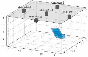
Figure 10: Overview

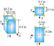
Figure 11: Feature Points

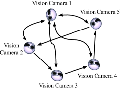
Figure 12: Communication Graph

We finally demonstrate the effectiveness of the networked visual motion observer and validity of the theoretical results through simulation. Throughout this section, we consider the situation where five pin-hole type vision cameras with focal length $0.01$[m] see a group of target objects. We identify the frame of camera 1 with the world frame and let $p_{w2}=[1\ 0\ 0]^{T},\ p_{w3}=[0\ 1\ 0]^{T},\ p_{w4}=[0\ -1\ 0]^{T},\ p_{w5}=[-1\ 0\ 0]^{T}$, and $e^{\hat{\xi}\theta_{wi}}=I_{3},\ {\forall i}\in\{2,3,4,5\}$. The overview of the setting is illustrated in Fig. 12, where blue boxes represent the initial configuration of target objects with $p_{wo_{1}}=[0.12\ 0.55\ -2.78],\ p_{wo_{2}}=[0.22\ 0.48\ -2.85],\ p_{wo_{3}}=[0.33\ 0.33\ -2.97],\ p_{wo_{4}}=[0.42\ 0.23\ -3.08],\ p_{wo_{5}}=[0.56\ 0.12\ -3.15]$ and $\xi\theta_{wo_{1}}=[-0.30\ -0.30\ -0.30],\ \xi\theta_{wo_{2}}=[-0.30\ -0.40\ -0.40],\ \xi\theta_{wo_{3}}=[-0.40\ -0.30\ -0.30],\ \xi\theta_{wo_{4}}=[-0.30\ -0.40\ -0.30],\ \xi\theta_{wo_{5}}=[-0.30\ -0.30\ -0.40].$ All the targets have four feature points whose positions relative to the object frame are illustrated in Fig. 12. We use the points projected onto the image plane as visual measurements $f_{i}$. The communication structure is depicted in Fig. 12 with $W=1$.

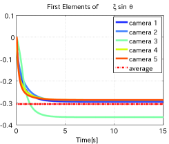
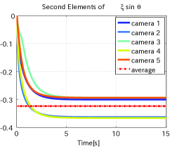
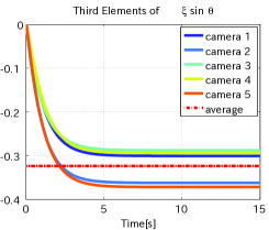
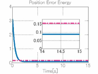
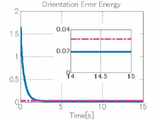
Figure 13: Time Responses of Each Element of $\bar{\xi}\sin\bar{\theta},\ i=1,\cdots,5$ (Static: $k_{s}=0.1$)

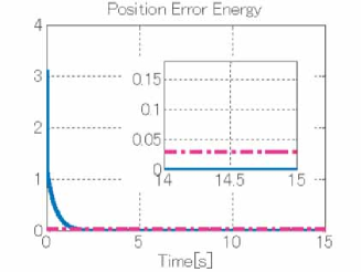
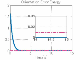
Figure 14: Time Response of $U_{p}$ (Left) and $U_{R}$ (Right) (Static: $k_{s}=0.1$)

Figure 15: Time Response of $U_{p}$ (Left) and $U_{R}$ (Right) (Static: $k_{s}=100$)

In the first scenario, we consider static target objects and demonstrate validity of Theorem 1. Then, the average $g^{*}=(p^{*},{e^{\hat{\xi}\theta^{*}}})$ is given by $p^{*}=[0.33\ 0.36\ -2.96],\ \xi\theta^{*}=[-0.32\ -0.34\ -0.34]$. For the configuration of the target objects, the parameter $\beta$ is given by about $\beta=0.86$. Throughout this section, we let the initial estimates be $\bar{p}_{io_{i}}(0)=[0\ 0\ 2.5]^{T}$ and ${e^{\hat{\bar{\xi}}\bar{\theta}_{io_{i}}}}(0)=I_{3}$.

We first employ the gains $k_{e}=1$ and $k_{s}=0.1$ ($k=10$). Then, the parameters $\varepsilon_{p}$ and $\varepsilon_{R}$ in Theorem 1 are given by $\varepsilon_{p}=\varepsilon_{R}=1$. Fig. 15 illustrates the time responses of orientation estimates of all vision cameras produced by the networked visual motion observer, where the red dash-dotted lines represent each element of the average $\xi^{*}\sin\theta^{*}$. We see from the figures that there exist gaps between the average and the estimates for all elements. The error functions $U_{p}$ and $U_{R}$ are depicted by blue curves in Fig. 15 respectively, where red dash dotted lines represent $\varepsilon_{p}\rho_{p}$ and $\varepsilon_{R}\rho_{R}$. Namely, Theorem 1 implies that the blue curve eventually takes lower values than the value indicated by the dash dotted line and we see that it is really achieved as expected.

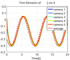
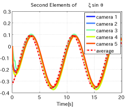
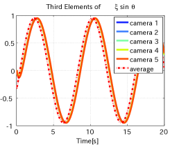
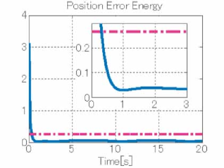
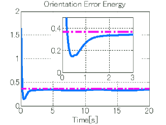
Figure 16: Time Responses of Each Element of $\bar{\xi}\sin\bar{\theta},\ i=1,\cdots,5$ (Moving: $k_{e}=3$)

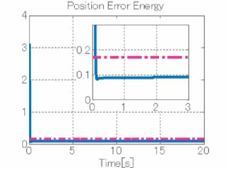
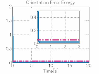
Figure 17: Time Responses of $U_{p}$ (Left) and $U_{R}$ (Right) (Moving: $k_{e}=3$)

Figure 18: Time Responses of $U_{p}$ (Left) and $U_{R}$ (Right) (Moving: $k_{e}=30$)

We next let $k_{e}=1$ and $k_{s}=100$ ($k=0.01$). Then, we have $\varepsilon_{p}=0.19,\ \varepsilon_{R}=0.31$ for sufficiently small $\epsilon$ and $c$. Fig. 15 illustrates the time responses of $U_{p}$ and $U_{R}$. We see from the figures that the estimates of all vision cameras become much closer to the average than the case of a small mutual feedback gain $k_{s}=0.1$. Fig. 15 also indicates that the error functions $U_{p}$ and $U_{R}$ ultimately take lower values than the right-hand side of (31) and (34) respectively. Namely, it turns out as predicted that a small $k=k_{e}/k_{s}$ results in a good averaging performance.

In the second scenario, we consider moving target objects with constant body velocities $V^{b}_{wo_{i}}=\begin{bmatrix}0.2&0&0&0&0&0.8\end{bmatrix}^{T}\ \ {\forall i}=1,\cdots,5$ and the same initial states as the above static case. For the targets, we apply the networked visual motion observer with $k_{e}=k_{s}=3$, where we let the initial estimates be the same as the above static object case. Then the time responses of orientation estimates are depicted in Fig. 18, where red dash dotted curves describe the average motion of the target orientations. We see from the figures that the estimates track the moving average within bounded errors and the networked observer also works for a dynamic problem.

The responses of $U_{p}$ and $U_{R}$ are illustrated in Fig. 18, where the dash-dotted lines show $\varepsilon_{p}^{\prime}\rho_{p}^{\prime}$ and $\varepsilon_{R}^{\prime}\rho_{R}^{\prime}$. As shown in Theorem 2, both of $U_{p}$ and $U_{R}$ ultimately take values smaller than $\varepsilon_{p}^{\prime}\rho_{p}^{\prime}$ and $\varepsilon_{R}^{\prime}\rho_{R}^{\prime}$ respectively. Their counterparts for $k_{e}=30,\ k_{s}=3$ are shown in Fig. 18, which also illustrate validity of Theorem 2. We also see that a large $k_{e}$ achieves a better tracking performance than a smaller $k_{e}$, which supports validity of the analysis at the end of Section V.

Experimental verifications on a testbed are omitted in this paper but shown in [27, 28].

VII Conclusions

This paper has presented a novel cooperative estimation mechanism for visual sensor networks. We have considered the situation where multiple smart vision cameras with computation and communication capability see a group of target objects. We first have presented an estimation mechanism called networked visual motion observer to meet two requirements, averaging and tracking. Then, we have derived an upper bound of the ultimate error between the actual average and the estimates produced by the present methodology. Moreover, we have derived an upper bound of the ultimate error from the estimates to the average when the target objects are moving. Finally, the effectiveness of the present mechanism has been demonstrated through simulation.

The authors would like to express sincere appreciation to Prof. Francesco Bullo and Prof. Kenji Hirata for their invaluable suggestions and advices.

Appendix A Proof of Lemma 1

In the proof, we use the following lemma.

Lemma 6

[15] For any matrices $R_{1},R_{2},R_{3}\in SO(3)$, the inequality

$$\frac{1}{2}{\rm tr}(R_{1}^{T}R_{2}-R_{1}^{T}R_{3}R_{2}^{T}R_{3})\geq\phi(R_{1}^{T}R_{3})-\phi(R_{1}^{T}R_{2})+\lambda_{min}({\rm sym}(R_{1}^{T}R_{3}))\phi(R_{3}^{T}R_{2})$$

holds, where ${\rm sym}(M):=\frac{1}{2}(M+M^{T})$ and $\lambda_{min}(M)$ is the minimal eigenvalue of matrix $M$.

The time evolution of the orientation estimate ${e^{\hat{\bar{\xi}}\bar{\theta}_{io_{i}}}}$ in (9) with $V^{b}_{wi}=0$ and (20) is given by

$${\dot{e}^{\hat{\bar{\xi}}\bar{\theta}_{io_{i}}}}={e^{\hat{\bar{\xi}}\bar{\theta}_{io_{i}}}}\hat{\omega}_{uei},\ {\omega}_{uei}=k_{e}e_{R}({e^{-\hat{\bar{\xi}}\bar{\theta}_{io_{i}}}}{e^{\hat{\xi}\theta_{io_{i}}}})+k_{s}\sum_{j\in{\mathcal{N}}_{i}}e_{R}({e^{-\hat{\bar{\xi}}\bar{\theta}_{io_{i}}}}{e^{\hat{\bar{\xi}}\bar{\theta}_{io_{j}}}}),$$ (39)

which is independent of evolution of the position estimate $\bar{p}_{io_{i}}$. Multiplying $e^{\hat{\xi}\theta_{wi}}$ to (39) from left, we have the following equation describing evolution of the estimate ${e^{\hat{\bar{\xi}}\bar{\theta}_{wo_{i}}}}$ relative to $\Sigma_{w}$.

$${\dot{e}^{\hat{\bar{\xi}}\bar{\theta}_{wo_{i}}}}={e^{\hat{\bar{\xi}}\bar{\theta}_{wo_{i}}}}\hat{\omega}_{uei},\ {\omega}_{uei}=k_{e}e_{R}({e^{-\hat{\bar{\xi}}\bar{\theta}_{wo_{i}}}}{e^{\hat{\xi}\theta_{wo_{i}}}})+k_{s}\sum_{j\in{\mathcal{N}}_{i}}e_{R}({e^{-\hat{\bar{\xi}}\bar{\theta}_{wo_{i}}}}{e^{\hat{\bar{\xi}}\bar{\theta}_{wo_{j}}}})$$ (40)

Let us now consider the energy function

$$U:=\phi({e^{-\hat{\xi}\theta_{\iota}^{*}}}{e^{\hat{\bar{\xi}}\bar{\theta}_{\iota o_{\iota}}}})=\phi({e^{-\hat{\xi}\theta^{*}}}{e^{\hat{\bar{\xi}}\bar{\theta}_{wo_{\iota}}}}),\ \iota(t):=\arg\max_{i\in{\mathcal{V}}}\phi({e^{-\hat{\xi}\theta_{i}^{*}}}{e^{\hat{\bar{\xi}}\bar{\theta}_{io_{i}}}}(t)).$$

Then, the time derivative of $U$ along with the trajectories of (40) is given by

$$\dot{U}=2e^{T}_{R}({e^{-\hat{\xi}\theta^{*}}}{e^{\hat{\bar{\xi}}\bar{\theta}_{wo_{\iota}}}})\omega_{ue\iota}=-{\rm tr}\left({\rm sk}({e^{-\hat{\xi}\theta^{*}}}{e^{\hat{\xi}\theta_{wo_{\iota}}}})\hat{\omega}_{ue\iota}\right),$$ (41)

where we use the relation $a^{T}b=-\frac{1}{2}{\rm tr}(\hat{a}\hat{b})$. Substituting (40) into (41) yields

$$\dot{U}=-{\rm tr}\Big{(}k_{e}\Big{(}{e^{-\hat{\xi}\theta^{*}}}{e^{\hat{\xi}\theta_{wo_{\iota}}}}-{e^{-\hat{\xi}\theta^{*}}}{e^{\hat{\bar{\xi}}\bar{\theta}_{wo_{\iota}}}}{e^{-\hat{\xi}\theta_{wo_{\iota}}}}{e^{\hat{\bar{\xi}}\bar{\theta}_{wo_{\iota}}}}\Big{)}$$

$$\hskip 56.9055pt+k_{s}\Big{(}\sum_{j\in\mathcal{N}_{\iota}}{e^{-\hat{\xi}\theta^{*}}}{e^{\hat{\bar{\xi}}\bar{\theta}_{wo_{\iota}}}}-{e^{-\hat{\xi}\theta^{*}}}{e^{\hat{\bar{\xi}}\bar{\theta}_{wo_{\iota}}}}{e^{-\hat{\bar{\xi}}\bar{\theta}_{wo_{j}}}}{e^{\hat{\bar{\xi}}\bar{\theta}_{wo_{\iota}}}}\Big{)}\Big{)}.$$ (42)

From Lemma 6, (42) is rewritten as $\dot{U}\leq-\left(k_{e}F_{1}+k_{s}F_{2}\right)$, where

$$F_{1}:=\phi({e^{-\hat{\xi}\theta^{*}}}{e^{\hat{\bar{\xi}}\bar{\theta}_{wo_{\iota}}}})-\phi({e^{-\hat{\xi}\theta^{*}}}{e^{\hat{\xi}\theta_{wo_{\iota}}}})+\sigma\phi({e^{-\hat{\bar{\xi}}\bar{\theta}_{wo_{\iota}}}}{e^{\hat{\xi}\theta_{wo_{\iota}}}}),\ \sigma:=\lambda_{min}({\rm sym}({e^{-\hat{\xi}\theta^{*}}}{e^{\hat{\bar{\xi}}\bar{\theta}_{wo_{\iota}}}})),$$

$$F_{2}:=\sum_{j\in\mathcal{N}_{\iota}}\Big{(}\phi({e^{-\hat{\xi}\theta^{*}}}{e^{\hat{\bar{\xi}}\bar{\theta}_{wo_{\iota}}}})-\phi({e^{-\hat{\xi}\theta^{*}}}{e^{\hat{\bar{\xi}}\bar{\theta}_{wo_{j}}}})+\sigma\phi({e^{\hat{\bar{\xi}}\bar{\theta}_{wo_{\iota}}}}{e^{\hat{\bar{\xi}}\bar{\theta}_{wo_{j}}}})\Big{)}.$$

From the definition of the index $\iota$, the inequality $\phi({e^{-\hat{\xi}\theta^{*}}}{e^{\hat{\bar{\xi}}\bar{\theta}_{wo_{\iota}}}})\geq\phi({e^{-\hat{\xi}\theta^{*}}}{e^{\hat{\bar{\xi}}\bar{\theta}_{wo_{j}}}})\ {\forall j}\in{\mathcal{V}}$ holds and hence we obtain $F_{2}\geq\sigma\sum_{j\in\mathcal{N}_{i}}\phi({e^{\hat{\bar{\xi}}\bar{\theta}_{wo_{\iota}}}}{e^{\hat{\bar{\xi}}\bar{\theta}_{wo_{j}}}})$. Thus, the inequality

$$\dot{U}\leq-\Big{(}k_{e}\phi({e^{-\hat{\xi}\theta^{*}}}{e^{\hat{\bar{\xi}}\bar{\theta}_{wo_{\iota}}}})-k_{e}\phi({e^{-\hat{\xi}\theta^{*}}}{e^{\hat{\xi}\theta_{wo_{\iota}}}})+\sigma\Big{(}k_{e}\phi({e^{-\hat{\bar{\xi}}\bar{\theta}_{wo_{\iota}}}}{e^{\hat{\xi}\theta_{wo_{\iota}}}})+k_{s}\sum_{j\in\mathcal{N}_{i}}\phi({e^{\hat{\bar{\xi}}\bar{\theta}_{wo_{\iota}}}}{e^{\hat{\bar{\xi}}\bar{\theta}_{wo_{j}}}})\Big{)}\Big{)}.$$

is true. From the assumption of ${e^{-\hat{\xi}\theta^{*}}}{e^{\hat{\bar{\xi}}\bar{\theta}_{wo_{i}}}}>0\ {\forall i}\in{\mathcal{V}}$, we have $\sigma>0$ and the inequality

$$\dot{U}\leq-k_{e}(\phi({e^{-\hat{\xi}\theta^{*}}}{e^{\hat{\bar{\xi}}\bar{\theta}_{wo_{\iota}}}})-\phi({e^{-\hat{\xi}\theta^{*}}}{e^{\hat{\xi}\theta_{wo_{\iota}}}}))\leq-k_{e}(\phi({e^{-\hat{\xi}\theta^{*}}}{e^{\hat{\bar{\xi}}\bar{\theta}_{wo_{\iota}}}})-\phi({e^{-\hat{\xi}\theta^{*}}}{e^{\hat{\xi}\theta_{wo_{h}}}})).$$

holds. Thus, if $\phi({e^{-\hat{\xi}\theta^{*}}}{e^{\hat{\bar{\xi}}\bar{\theta}_{wo_{\iota}}}})-\phi({e^{-\hat{\xi}\theta^{*}}}{e^{\hat{\xi}\theta_{wo_{h}}}})>c$, then $\dot{U}\leq-ck_{e}$ is true. Namely, there exists a finite $\tau(c)$ such that ${e^{\hat{\bar{\xi}}\bar{\theta}_{wo_{\iota}}}}$ satisfies $\phi({e^{-\hat{\xi}\theta^{*}}}{e^{\hat{\bar{\xi}}\bar{\theta}_{wo_{\iota}}}})-\phi({e^{-\hat{\xi}\theta^{*}}}{e^{\hat{\xi}\theta_{wo_{h}}}})<c\ {\forall t}\geq\tau(c)$ and, from the definition of $\iota$, we also have $\phi({e^{-\hat{\xi}\theta^{*}}}{e^{\hat{\bar{\xi}}\bar{\theta}_{wo_{i}}}})-\phi({e^{-\hat{\xi}\theta^{*}}}{e^{\hat{\xi}\theta_{wo_{h}}}})<c\ {\forall t}\geq\tau(c)$ for all $i\in{\mathcal{V}}$. This completes the proof.

Appendix B Proof of Lemma 2

In the proof, we use the energy functions

$$\ \ U_{p}:=\frac{1}{2}\sum_{i\in{\mathcal{V}}}\|p_{i}^{*}-\bar{p}_{io_{i}}\|^{2}=\frac{1}{2}\sum_{i\in{\mathcal{V}}}\|p^{*}-\bar{p}_{wo_{i}}\|^{2},\ U_{R}:=\sum_{i\in{\mathcal{V}}}\phi({e^{-\hat{\xi}\theta_{i}^{*}}}{e^{\hat{\bar{\xi}}\bar{\theta}_{io_{i}}}})=\sum_{i\in{\mathcal{V}}}\phi({e^{-\hat{\xi}\theta^{*}}}{e^{\hat{\bar{\xi}}\bar{\theta}_{wo_{i}}}}).$$

We first consider evolution of the position estimates $(\bar{p}_{io_{i}})_{i\in{\mathcal{V}}}$ and then show its counterpart with respect to orientation estimates $({e^{\hat{\bar{\xi}}\bar{\theta}_{io_{i}}}})_{i\in{\mathcal{V}}}$ separately. The time evolution of the position estimate $\bar{p}_{io_{i}}$ in (9) with $V^{b}_{wi}=0$ and (20) is described by $\dot{\bar{p}}_{io_{i}}=k_{e}(p_{io_{i}}-\bar{p}_{io_{i}})+k_{s}\sum_{j\in{\mathcal{N}}_{i}}(\bar{p}_{io_{j}}-\bar{p}_{io_{i}})$. Since the cameras are static, the evolution of $\bar{p}_{wo_{i}}$ relative to the world frame $\Sigma_{w}$ is given by

$$\dot{\bar{p}}_{wo_{i}} \!\!\!=\!\!\! e^{\hat{\xi}\theta_{wi}}\dot{\bar{p}}_{io_{i}}=k_{e}(p_{wo_{i}}-\bar{p}_{wo_{i}})+k_{s}\sum_{j\in{\mathcal{N}}_{i}}(\bar{p}_{wo_{j}}-\bar{p}_{wo_{i}}),$$ (43)

which is independent of evolution of the orientation estimates (40).

If we define $\bar{q}_{i}:=\bar{p}_{wo_{i}}-p^{*}$ and ${q}_{i}:={p}_{wo_{i}}-p^{*}$, the time derivative of $U_{p}$ along with the trajectories of (43) is given by

$$\dot{U}_{p} \!\!\!=\!\!\! \sum_{i\in{\mathcal{V}}}\left(k_{e}\bar{q}_{i}^{T}(q_{i}-\bar{q}_{i})+k_{s}\sum_{j\in{\mathcal{N}}_{i}}\bar{q}_{i}^{T}(\bar{q}_{j}-\bar{q}_{i})\right)$$

$$\!\!\!=\!\!\! \frac{1}{2}\sum_{i\in{\mathcal{V}}}\Big{(}k_{e}(\|q_{i}\|^{2}-\|\bar{q}_{i}\|^{2}-\|q_{i}-\bar{q}_{i}\|^{2})+k_{s}\sum_{j\in{\mathcal{N}}_{i}}(\|\bar{q}_{j}\|^{2}-\|\bar{q}_{i}\|^{2}-\|\bar{q}_{j}-\bar{q}_{i}\|^{2})\Big{)}.$$

Since $\sum_{i\in{\mathcal{V}}}\sum_{j\in\mathcal{N}_{i}}\|\bar{q}_{j}\|^{2}-\|\bar{q}_{i}\|^{2}=0$ holds under Assumption 1 [15], we obtain

$$\dot{U}_{p} \!\!\!=\!\!\! \frac{1}{2}\sum_{i\in{\mathcal{V}}}\Big{(}k_{e}(\|q_{i}\|^{2}-\|\bar{q}_{i}\|^{2}-\|q_{i}-\bar{q}_{i}\|^{2})-k_{s}\sum_{j\in{\mathcal{N}}_{i}}\|\bar{q}_{j}-\bar{q}_{i}\|^{2}\Big{)}.$$ (44)

We see from (44) that if $(\bar{p}_{io_{i}})_{i\in{\mathcal{V}}}\in\Omega_{p}(1)$ then

$$\dot{U}_{p}\leq-\frac{1}{2}\sum_{i\in{\mathcal{V}}}\Big{(}k_{e}\|q_{i}-\bar{q}_{i}\|^{2}+k_{s}\sum_{j\in{\mathcal{N}}_{i}}\|\bar{q}_{j}-\bar{q}_{i}\|^{2}\Big{)}$$ (45)

holds. From Assumption 2, $\sum_{i\in{\mathcal{V}}}\|q_{i}-\bar{q}_{i}\|^{2}$ and $\sum_{i\in{\mathcal{V}}}\sum_{j\in{\mathcal{N}}_{i}}\|\bar{q}_{j}-\bar{q}_{i}\|^{2}$ are never equal to $0$ simultaneously and hence the right-hand side of (45) is strictly negative. Thus, the trajectories of the position estimates $(\bar{p}_{io_{i}})_{i\in{\mathcal{V}}}$ along with (43) settle into the set $\Omega_{p}(1)$ in finite time.

The time derivative of $U_{R}$ along the trajectories of (40) is given by

$$\dot{U}_{R}=2\sum_{i\in{\mathcal{V}}}e^{T}_{R}({e^{-\hat{\xi}\theta^{*}}}{e^{\hat{\bar{\xi}}\bar{\theta}_{wo_{i}}}}){\omega}_{uei},=-\sum_{i\in{\mathcal{V}}}{\rm tr}\left({\rm sk}({e^{-\hat{\xi}\theta^{*}}}{e^{\hat{\bar{\xi}}\bar{\theta}_{wo_{i}}}})\hat{\omega}_{uei}\right).$$ (46)

Substituting (40) into (46) yields

$$\dot{U}_{R}=-\sum_{i\in{\mathcal{V}}}{\rm tr}(k_{e}\Phi_{1}+k_{s}\Phi_{2}),$$ (47)

$$\Phi_{1}:=\frac{1}{2}({e^{-\hat{\xi}\theta^{*}}}{e^{\hat{\xi}\theta_{wo_{i}}}}-{e^{-\hat{\xi}\theta^{*}}}{e^{\hat{\bar{\xi}}\bar{\theta}_{wo_{i}}}}{e^{-\hat{\xi}\theta_{wo_{i}}}}{e^{\hat{\bar{\xi}}\bar{\theta}_{wo_{i}}}}),$$

$$\Phi_{2}:=\frac{1}{2}\sum_{j\in{\mathcal{N}}_{i}}\left({e^{-\hat{\xi}\theta^{*}}}{e^{\hat{\bar{\xi}}\bar{\theta}_{wo_{j}}}}-{e^{-\hat{\xi}\theta^{*}}}{e^{\hat{\bar{\xi}}\bar{\theta}_{wo_{i}}}}{e^{-\hat{\bar{\xi}}\bar{\theta}_{wo_{j}}}}{e^{\hat{\bar{\xi}}\bar{\theta}_{wo_{i}}}}\right).$$

We first consider the term $\sum_{i}{\rm tr}(\Phi_{2})$ in (47). From Lemma 6, the following inequality holds.

$$\sum_{i\in{\mathcal{V}}}{\rm tr}(\Phi_{2})\geq\sum_{i\in{\mathcal{V}}}\sum_{j\in{\mathcal{N}}_{i}}\left\{\phi({e^{-\hat{\xi}\theta^{*}}}{e^{\hat{\bar{\xi}}\bar{\theta}_{wo_{i}}}})-\phi({e^{-\hat{\xi}\theta^{*}}}{e^{\hat{\bar{\xi}}\bar{\theta}_{wo_{j}}}})+\sigma_{i}\phi({e^{-\hat{\bar{\xi}}\bar{\theta}_{wo_{i}}}}{e^{\hat{\bar{\xi}}\bar{\theta}_{wo_{j}}}})\right\},$$ (48)

where $\sigma_{i}:=\lambda_{min}({\rm sym}({e^{-\hat{\xi}\theta^{*}}}{e^{\hat{\bar{\xi}}\bar{\theta}_{wo_{i}}}}))$. Assumption 1 implies that $\sum_{i\in{\mathcal{V}}}\sum_{j\in{\mathcal{N}}_{i}}\phi({e^{-\hat{\xi}\theta^{*}}}{e^{\hat{\bar{\xi}}\bar{\theta}_{wo_{i}}}})-\phi({e^{-\hat{\xi}\theta^{*}}}{e^{\hat{\bar{\xi}}\bar{\theta}_{wo_{j}}}})=0$ [15] and hence (48) is rewritten as

$$\sum_{i\in{\mathcal{V}}}{\rm tr}(\Phi_{2})\geq\sum_{i\in{\mathcal{V}}}\sum_{j\in{\mathcal{N}}_{i}}\sigma_{i}\phi({e^{-\hat{\bar{\xi}}\bar{\theta}_{wo_{i}}}}{e^{\hat{\bar{\xi}}\bar{\theta}_{wo_{j}}}}).$$ (49)

We next consider the term $k_{e}\sum_{i\in{\mathcal{V}}}{\rm tr}(\Phi_{1})$ in (47). Applying Lemma 6 again to the term yields

$$\sum_{i\in{\mathcal{V}}}{\rm tr}(\Phi_{1})\geq\sum_{i\in{\mathcal{V}}}\left\{\phi({e^{-\hat{\xi}\theta^{*}}}{e^{\hat{\bar{\xi}}\bar{\theta}_{wo_{i}}}})-\phi({e^{-\hat{\xi}\theta^{*}}}{e^{\hat{\xi}\theta_{wo_{i}}}})+\sigma_{i}\phi({e^{-\hat{\bar{\xi}}\bar{\theta}_{wo_{i}}}}{e^{\hat{\xi}\theta_{wo_{i}}}})\right\}.$$ (50)

Substituting (49) and (50) into (47) yields

$$\dot{U}_{R}\leq-\sum_{i\in{\mathcal{V}}}\Big{(}k_{e}\phi({e^{-\hat{\xi}\theta^{*}}}{e^{\hat{\bar{\xi}}\bar{\theta}_{wo_{i}}}})-k_{e}\phi({e^{-\hat{\xi}\theta^{*}}}{e^{\hat{\xi}\theta_{wo_{i}}}})$$

$$\hskip 142.26378pt+\sigma_{i}\Big{(}k_{e}\phi({e^{-\hat{\bar{\xi}}\bar{\theta}_{wo_{i}}}}{e^{\hat{\xi}\theta_{wo_{i}}}})+k_{s}\sum_{j\in{\mathcal{N}}_{i}}\phi({e^{-\hat{\bar{\xi}}\bar{\theta}_{wo_{i}}}}{e^{\hat{\bar{\xi}}\bar{\theta}_{wo_{j}}}})\Big{)}\Big{)}.$$ (51)

If $({e^{\hat{\bar{\xi}}\bar{\theta}_{io_{i}}}})_{i\in{\mathcal{V}}}\notin\Omega_{R}(1)$ is true, (51) is rewritten as

$$\dot{U}_{R}\leq-\sum_{i\in{\mathcal{V}}}\sigma_{i}\Big{(}k_{e}\phi({e^{-\hat{\bar{\xi}}\bar{\theta}_{wo_{i}}}}{e^{\hat{\xi}\theta_{wo_{i}}}})+k_{s}\sum_{j\in{\mathcal{N}}_{i}}\phi({e^{-\hat{\bar{\xi}}\bar{\theta}_{wo_{i}}}}{e^{\hat{\bar{\xi}}\bar{\theta}_{wo_{j}}}})\Big{)}.$$ (52)

Note that, from the assumption of ${e^{-\hat{\xi}\theta^{*}}}{e^{\hat{\bar{\xi}}\bar{\theta}_{wo_{i}}}}>0$, we have $\sigma_{i}>0$. Since both of the terms $\sum_{i\in{\mathcal{V}}}\sigma_{i}\phi({e^{-\hat{\bar{\xi}}\bar{\theta}_{wo_{i}}}}{e^{\hat{\xi}\theta_{wo_{i}}}})$ and $\sum_{i\in{\mathcal{V}}}\sigma_{i}\sum_{j\in{\mathcal{N}}_{i}}\phi({e^{-\hat{\bar{\xi}}\bar{\theta}_{wo_{i}}}}{e^{\hat{\bar{\xi}}\bar{\theta}_{wo_{j}}}})$ are never equal to $0$ under Assumption 2, the right-hand side of (52) is strictly negative. This implies that the trajectories of the estimates $({e^{\hat{\bar{\xi}}\bar{\theta}_{io_{i}}}})_{i\in{\mathcal{V}}}$ converge to the set $\Omega_{R}(1)$ in finite time.

Appendix C Proof of Lemma 3

Suppose that $\phi({e^{-\hat{\xi}\theta^{*}}}{e^{\hat{\bar{\xi}}\bar{\theta}_{wo_{i}}}})<\phi({e^{-\hat{\xi}\theta^{*}}}{e^{\hat{\xi}\theta_{wo_{h}}}})+c$ holds true for some $c>0$. Then, from Hoff-man-Wielandt’s perturbation theorem [33], we have

$$\left|\lambda_{min}({\rm sym}({e^{-\hat{\xi}\theta^{*}}}{e^{\hat{\bar{\xi}}\bar{\theta}_{wo_{i}}}}))-\lambda_{min}({\rm sym}({e^{-\hat{\xi}\theta^{*}}}{e^{\hat{\xi}\theta^{*}}}))\right|\leq\left\|{\rm sym}({e^{-\hat{\xi}\theta^{*}}}{e^{\hat{\bar{\xi}}\bar{\theta}_{wo_{i}}}})-{\rm sym}({e^{-\hat{\xi}\theta^{*}}}{e^{\hat{\xi}\theta^{*}}})\right\|_{F}$$

$$\hskip 85.35826pt\leq\|{e^{-\hat{\xi}\theta^{*}}}({e^{\hat{\bar{\xi}}\bar{\theta}_{wo_{i}}}}-{e^{\hat{\xi}\theta^{*}}})\|_{F}=\|{e^{\hat{\bar{\xi}}\bar{\theta}_{wo_{i}}}}-{e^{\hat{\xi}\theta^{*}}}\|_{F}<\sqrt{2(\phi({e^{-\hat{\xi}\theta^{*}}}{e^{\hat{\xi}\theta_{wo_{h}}}})+c)}.$$

This immediately means

$$\lambda_{min}({\rm sym}({e^{-\hat{\xi}\theta^{*}}}{e^{\hat{\bar{\xi}}\bar{\theta}_{wo_{i}}}}))\geq\beta:=1-\sqrt{2(\phi({e^{-\hat{\xi}\theta^{*}}}{e^{\hat{\xi}\theta_{wo_{h}}}})+c)}.$$ (53)

From Lemma 1 and (53), Inequality (51) is rewritten as

$$\dot{U}_{R}\leq-\sum_{i\in{\mathcal{V}}}\Big{(}k_{e}\phi({e^{-\hat{\xi}\theta^{*}}}{e^{\hat{\bar{\xi}}\bar{\theta}_{wo_{i}}}})-k_{e}\phi({e^{-\hat{\xi}\theta^{*}}}{e^{\hat{\xi}\theta_{wo_{i}}}})$$

$$\hskip 85.35826pt+\beta\Big{(}k_{e}\phi({e^{-\hat{\bar{\xi}}\bar{\theta}_{wo_{i}}}}{e^{\hat{\xi}\theta_{wo_{i}}}})+k_{s}\sum_{j\in{\mathcal{N}}_{i}}\phi({e^{-\hat{\bar{\xi}}\bar{\theta}_{wo_{i}}}}{e^{\hat{\bar{\xi}}\bar{\theta}_{wo_{j}}}})\Big{)}\Big{)}$$ (54)

at least after the time $\tau(c)$. If $({e^{\hat{\bar{\xi}}\bar{\theta}_{io_{i}}}})_{i\in{\mathcal{V}}}\in{\mathcal{S}}^{R}_{2}(k)$ holds true, then we have

$$\dot{U}_{R}\leq-k_{e}\sum_{i\in{\mathcal{V}}}\Big{(}\phi({e^{-\hat{\xi}\theta^{*}}}{e^{\hat{\bar{\xi}}\bar{\theta}_{wo_{i}}}})+\beta\phi({e^{-\hat{\bar{\xi}}\bar{\theta}_{wo_{i}}}}{e^{\hat{\xi}\theta_{wo_{i}}}})\Big{)}$$ (55)

at least after the time $\tau(c)$. Under Assumption 2, the right-hand side of (55) is strictly negative.

In terms of $U_{p}$, from (44), if $(\bar{p}_{io_{i}})_{i\in{\mathcal{V}}}\in{\mathcal{S}}^{p}_{2}(k)$, we have $\dot{U}_{p}=-\frac{k_{e}}{2}\sum_{i\in{\mathcal{V}}}\Big{(}\|\bar{q}_{i}\|^{2}+\|q_{i}-\bar{q}_{i}\|^{2}\Big{)}$, whose right-hand side is strictly negative under Assumption 2. These complete the proof.

Appendix D Proof of Theorem 1

We first consider evolution of the position estimates $(\bar{p}_{io_{i}})_{i\in{\mathcal{V}}}$ described by (43). The case not satisfying $k\leq 1/W$ is already proved in Lemma 2 and hence we consider the case such that $k\leq 1/W$ is satisfied. Lemmas 2 and 3 indicate that $\dot{U}_{p}<0$ holds in $\Omega_{p}(1)\cup{\mathcal{S}}^{p}_{2}(k)$. Namely, from the inclusion (28), we have $\dot{U}_{p}<0$ except for the region $\Omega_{p}({\varepsilon_{p}})$ if $\dot{U}_{p}<0$ holds in the region ${\mathcal{S}}_{3}^{p}(k,\varepsilon_{p})$. If it is true, the trajectories along with (43) settle into the set $\Omega_{p}({\varepsilon_{p}})$ in finite time. It is thus sufficient to prove that $\dot{U}_{p}$ is strictly negative for all $(\bar{p}_{io_{i}})_{i\in{\mathcal{V}}}\in{\mathcal{S}}_{3}^{p}(k,\varepsilon_{p})$.

Equation (44) is rewritten as

$$\dot{U}_{p} \!\!\!=\!\!\! -\frac{k_{e}}{2}\sum_{i\in{\mathcal{V}}}\Big{(}-\|{q}_{i}\|^{2}+\|\bar{q}_{i}\|^{2}+(1-\epsilon)\|{q}_{i}-\bar{q}_{i}\|^{2}\Big{)}-a_{p},$$ (56)

where $a_{p}:=\frac{1}{2}\sum_{i\in{\mathcal{V}}}\Big{(}k_{e}\epsilon\|q_{i}-\bar{q}_{i}\|^{2}+k_{s}\sum_{j\in{\mathcal{N}}_{i}}\|\bar{q}_{j}-\bar{q}_{i}\|^{2}\Big{)}$ is strictly positive under Assumption 2. Now, for any $\alpha\in(0,1)$ and $j^{*}\in{\mathcal{V}}$, we have

$$\|q_{i}-\bar{q}_{i}\|^{2} \!\!\!\geq\!\!\! \alpha\|q_{i}-\bar{q}_{j^{*}}\|^{2}-\frac{\alpha}{1-\alpha}\|\bar{q}_{i}-\bar{q}_{j^{*}}\|^{2}.$$ (57)

Let $j^{*}$ be a node satisfying $j^{*}=\arg\min_{i_{0}}D(i_{0})$ and $G_{T}^{*}=({\mathcal{V}},{\mathcal{E}}_{T}^{*})\in{\mathcal{T}}(j^{*})$ be a graph satisfying $G_{T}^{*}=\arg\min_{G_{T}\in{\mathcal{T}}(j^{*})}\tilde{D}(G_{T})$, where $D$ and $\tilde{D}$ are defined in (4). Then, we obtain

$$\ \ \|\bar{q}_{i}-\bar{q}_{j^{*}}\|^{2}=\Big{\|}\sum_{l\in\{0,\cdots,d_{G^{*}_{T}}(i)-1\}}(\bar{q}_{v_{l}(i)}-\bar{q}_{v_{l+1}(i)})\Big{\|}^{2}\leq d_{G^{*}_{T}}(i)\sum_{l\in\{0,\cdots,d_{G^{*}_{T}}(i)-1\}}\|\bar{q}_{v_{l}(i)}-\bar{q}_{v_{l+1}(i)}\|^{2},$$

where $(v_{0}(i),\cdots,v_{d_{G^{*}_{T}}(i)-1}(i))$ is the path from root $j^{*}$ to node $i$ along tree $G_{T}^{*}$. Namely,

$$\sum_{i\in{\mathcal{V}}}\|\bar{q}_{i}-\bar{q}_{j^{*}}\|^{2}\leq\sum_{i\in{\mathcal{V}}}d_{G^{*}_{T}}(i)\sum_{l\in\{0,\cdots,d_{G^{*}_{T}}(i)-1\}}\|\bar{q}_{v_{l}(i)}-\bar{q}_{v_{l+1}(i)}\|^{2}.$$ (58)

holds. For any edge $E=(v^{1},v^{2})$ of $G_{T}^{*}$, the coefficient of $\|\bar{q}_{v^{1}}-\bar{q}_{v^{2}}\|^{2}$ in the right hand side of (58) is given by $\sum_{i\in{\mathcal{V}}}\delta_{G^{*}_{T}}(E;i)d_{G^{*}_{T}}(i)$, which is upper-bounded by $\tilde{D}(G^{*}_{T})=W$. We thus have

$$\sum_{i\in{\mathcal{V}}}\|\bar{q}_{i}-\bar{q}_{j^{*}}\|^{2}\leq W\sum_{E=(v^{1},v^{2})\in{\mathcal{E}}_{T}^{*}}\|\bar{q}_{v^{1}}-\bar{q}_{v^{2}}\|^{2}\leq W\sum_{i\in{\mathcal{V}}}\sum_{j\in\mathcal{N}_{i}}\|\bar{q}_{i}-\bar{q}_{j}\|^{2}.$$ (59)

The latter inequality of (59) holds because $G^{*}_{T}$ is a subgraph of $G_{u}$. Since $(\bar{p}_{io_{i}})_{i\in{\mathcal{V}}}\in{\mathcal{S}}_{3}^{p}(k,\varepsilon_{p})$, the inclusion $(\bar{p}_{io_{i}})_{i\in{\mathcal{V}}}\notin{\mathcal{S}}^{p}_{2}(k)$ holds and hence

$$\sum_{i\in{\mathcal{V}}}\sum_{j\in\mathcal{N}_{i}}\|\bar{q}_{i}-\bar{q}_{j}\|^{2}=\sum_{i\in{\mathcal{V}}}\sum_{j\in\mathcal{N}_{i}}\|\bar{p}_{wo_{i}}-\bar{p}_{wo_{j}}\|^{2}\leq 2k\rho_{p}.$$ (60)

Moreover, the following inequality holds from the definition of the average $p^{*}$.

$$\sum_{i\in{\mathcal{V}}}\|q_{i}-\bar{q}_{j^{*}}\|^{2}=\sum_{i\in{\mathcal{V}}}\|p_{wo_{i}}-\bar{p}_{wo_{j^{*}}}\|^{2}\geq\sum_{i\in{\mathcal{V}}}\|p_{wo_{i}}-p^{*}\|^{2}=2\rho_{p}$$ (61)

From (57), (59), (60) and (61), equation (56) is rewritten as

$$\dot{U}_{p} \!\!\!\leq\!\!\! {k_{e}}\left\{-\frac{1}{2}\Big{(}\sum_{i\in{\mathcal{V}}}\|\bar{q}_{i}\|^{2}\Big{)}+\Big{(}1-(1-\epsilon)\Big{(}\alpha-\frac{kW\alpha}{1-\alpha}\Big{)}\Big{)}\rho_{p}\right\}-a_{p}.$$ (62)

If $(\bar{p}_{io_{i}})_{i\in{\mathcal{V}}}\in{\mathcal{S}}_{3}^{p}(k,\varepsilon_{p})$, then $(\bar{p}_{io_{i}})_{i\in{\mathcal{V}}}\notin\Omega_{p}(\varepsilon_{p})$ and hence (62) is rewritten as

$$\dot{U}_{p} \!\!\!\leq\!\!\! {k_{e}}\left\{(1-\epsilon)\Big{(}\alpha-\frac{kW\alpha}{1-\alpha}-\left(1-\sqrt{kW}\right)^{2}\Big{)}\right\}\rho_{p}-a_{p}.$$

Under the assumption that $k\leq 1/W$, the inequality $\alpha-\frac{kW\alpha}{1-\alpha}\leq\left(1-\sqrt{kW}\right)^{2}$ holds for any $\alpha\in(0,1)$ and hence $\dot{U}_{p}\leq-a_{p}<0$. This completes the proof of the former half of the theorem.

We next consider the evolution of the orientation estimates $({e^{\hat{\bar{\xi}}\bar{\theta}_{io_{i}}}})_{i\in{\mathcal{V}}}$ described by (40). The case not satisfying $k\leq\beta/W$ or $\beta>0$ is already proved in Lemma 2. We thus consider the case such that $k\leq\beta/W$ and $\beta>0$ hold. We first note that the set ${\mathcal{S}}=\{({e^{\hat{\bar{\xi}}\bar{\theta}_{io_{i}}}})_{i\in{\mathcal{V}}}|\ {e^{-\hat{\bar{\xi}}\bar{\theta}_{io_{i}}}}{e^{\hat{\xi}\theta_{i}^{*}}}>0\ {\forall i}\in{\mathcal{V}}\}$ is a positively invariant set from Lemma 1 and hence trajectories of $({e^{\hat{\bar{\xi}}\bar{\theta}_{io_{i}}}})_{i\in{\mathcal{V}}}$ starting from ${\mathcal{S}}$ never gets out of ${\mathcal{S}}$. Lemmas 2 and 3 also prove that, in the region ${\mathcal{S}}$, $\dot{U}_{R}<0$ holds if $({e^{\hat{\bar{\xi}}\bar{\theta}_{io_{i}}}})_{i\in{\mathcal{V}}}\in({\mathcal{S}}\setminus\Omega_{R}(1))\cup{\mathcal{S}}^{R}_{2}(k)$ at least after the time $\tau(c)$. Namely, as long as $\dot{U}_{R}<0$ is true in the region ${\mathcal{S}}_{3}^{R}(k,\varepsilon_{R})$, the inequality $\dot{U}_{R}<0$ holds except for the region $\Omega_{R}({\varepsilon_{R}})$ from the inclusion (28), which means the trajectories along with (40) settle into the set $\Omega_{R}({\varepsilon_{R}})$ in finite time. It is thus sufficient to prove that $\dot{U}_{R}$ is strictly negative for all $({e^{\hat{\bar{\xi}}\bar{\theta}_{io_{i}}}})_{i\in{\mathcal{V}}}\in{\mathcal{S}}_{3}^{R}(k,\varepsilon_{R})$.

We first notice that if we define $a_{R}:=\beta\sum_{i\in{\mathcal{V}}}\Big{(}k_{e}\epsilon\phi({e^{-\hat{\bar{\xi}}\bar{\theta}_{wo_{i}}}}{e^{\hat{\xi}\theta_{wo_{i}}}})+k_{s}\sum_{j\in{\mathcal{N}}_{i}}\phi({e^{-\hat{\bar{\xi}}\bar{\theta}_{wo_{i}}}}{e^{\hat{\bar{\xi}}\bar{\theta}_{wo_{j}}}})\Big{)}$, $a_{R}$ is strictly positive under Assumption 2. Using the parameter $a_{R}$, (54) is rewritten as

$$\dot{U}_{R} \!\!\!\leq\!\!\! -k_{e}\sum_{i\in{\mathcal{V}}}\Big{(}-\phi({e^{-\hat{\xi}\theta^{*}}}{e^{\hat{\xi}\theta_{wo_{i}}}})+\phi({e^{-\hat{\xi}\theta^{*}}}{e^{\hat{\bar{\xi}}\bar{\theta}_{wo_{i}}}})+\beta(1-\epsilon)\phi({e^{-\hat{\bar{\xi}}\bar{\theta}_{wo_{i}}}}{e^{\hat{\xi}\theta_{wo_{i}}}})\Big{)}-a_{R}.$$ (63)

We thus consider the former three terms of the right hand side of Inequality (63). We first have

$$\phi({e^{-\hat{\bar{\xi}}\bar{\theta}_{wo_{i}}}}{e^{\hat{\xi}\theta_{wo_{i}}}}) \!\!\!\geq\!\!\! \alpha\phi({e^{-\hat{\bar{\xi}}\bar{\theta}_{wo_{j^{*}}}}}{e^{\hat{\xi}\theta_{wo_{i}}}})-\frac{\alpha}{1-\alpha}\phi({e^{-\hat{\bar{\xi}}\bar{\theta}_{wo_{j^{*}}}}}{e^{\hat{\bar{\xi}}\bar{\theta}_{wo_{i}}}})$$ (64)

for any $\alpha\in(0,1)$ and $j^{*}\in{\mathcal{V}}$. Again, let $j^{*}$ be a node satisfying $j^{*}=\arg\min_{i_{0}}D(i_{0})$ and $G^{*}_{T}=({\mathcal{V}},{\mathcal{E}}_{T}^{*})\in{\mathcal{T}}(j^{*})$ be a graph satisfying $G^{*}_{T}=\arg\min_{G_{T}\in{\mathcal{T}}(j^{*})}\tilde{D}(G_{T})$. Then, the inequality

$$\phi({e^{-\hat{\bar{\xi}}\bar{\theta}_{wo_{j^{*}}}}}{e^{\hat{\bar{\xi}}\bar{\theta}_{wo_{i}}}})\leq d_{G^{*}_{T}}(i)\sum_{l\in\{0,\cdots,d_{G^{*}_{T}}(i)-1\}}\phi(e^{-\hat{\bar{\xi}}\bar{\theta}_{wo_{v_{l}(i)}}}e^{\hat{\bar{\xi}}\bar{\theta}_{wo_{v_{l+1}(i)}}})$$ (65)

holds from the definition of the energy function $\phi$ and hence

$$\sum_{i\in{\mathcal{V}}}\phi({e^{-\hat{\bar{\xi}}\bar{\theta}_{wo_{j^{*}}}}}{e^{\hat{\bar{\xi}}\bar{\theta}_{wo_{i}}}})\leq\sum_{i\in{\mathcal{V}}}d_{G_{T}^{*}}(i)\sum_{l\in\{0,\cdots,d_{G^{*}_{T}}(i)-1\}}\phi(e^{-\hat{\bar{\xi}}\bar{\theta}_{wo_{v_{l}(i)}}}e^{\hat{\bar{\xi}}\bar{\theta}_{wo_{v_{l+1}(i)}}}).$$ (66)

Similarly to the case of position estimates, (66) is rewritten as

$$\sum_{i\in{\mathcal{V}}}\phi({e^{-\hat{\bar{\xi}}\bar{\theta}_{wo_{j^{*}}}}}{e^{\hat{\bar{\xi}}\bar{\theta}_{wo_{i}}}})\leq W\sum_{E=(v^{1},v^{2})\in{\mathcal{E}}_{T}}\phi(e^{-\hat{\bar{\xi}}\bar{\theta}_{wo_{v^{1}}}}e^{\hat{\bar{\xi}}\bar{\theta}_{wo_{v^{2}}}})\leq W\sum_{i\in{\mathcal{V}}}\sum_{j\in\mathcal{N}_{i}}\phi({e^{-\hat{\bar{\xi}}\bar{\theta}_{wo_{i}}}}{e^{\hat{\bar{\xi}}\bar{\theta}_{wo_{j}}}}).$$ (67)

Since $({e^{\hat{\bar{\xi}}\bar{\theta}_{io_{i}}}})_{i\in{\mathcal{V}}}\in{\mathcal{S}}_{3}^{R}(k,\varepsilon_{R})$, the inclusion $({e^{\hat{\bar{\xi}}\bar{\theta}_{io_{i}}}})_{i\in{\mathcal{V}}}\notin{\mathcal{S}}^{R}_{2}(k)$ holds and hence

$$\sum_{i\in{\mathcal{V}}}\sum_{j\in\mathcal{N}_{i}}\phi({e^{-\hat{\bar{\xi}}\bar{\theta}_{wo_{i}}}}{e^{\hat{\bar{\xi}}\bar{\theta}_{wo_{j}}}})\leq\frac{k\rho_{R}}{\beta}$$ (68)

is true. We next focus on $\phi({e^{-\hat{\bar{\xi}}\bar{\theta}_{wo_{j^{*}}}}}{e^{\hat{\xi}\theta_{wo_{i}}}})$ in (64). From the definition of the average ${e^{\hat{\xi}\theta^{*}}}$ (7),

$$\sum_{i\in{\mathcal{V}}}\phi({e^{-\hat{\bar{\xi}}\bar{\theta}_{wo_{j^{*}}}}}{e^{\hat{\xi}\theta_{wo_{i}}}})\geq\sum_{i\in{\mathcal{V}}}\phi({e^{-\hat{\xi}\theta^{*}}}{e^{\hat{\xi}\theta_{wo_{i}}}})=\rho_{R}$$ (69)

holds for any ${e^{\hat{\bar{\xi}}\bar{\theta}_{wo_{j}}}}\in SO(3)$. Substituting (64), (67), (68) and (69) into inequality (63) yields

$$\dot{U}_{R}\leq-k_{e}\Big{\{}\Big{(}\sum_{i\in{\mathcal{V}}}\phi({e^{-\hat{\xi}\theta^{*}}}{e^{\hat{\bar{\xi}}\bar{\theta}_{wo_{i}}}})\Big{)}-\Big{(}1-(1-\epsilon)\Big{(}\alpha\beta-\frac{kW\alpha}{1-\alpha}\Big{)}\Big{)}\rho_{R}\Big{\}}-a_{R}.$$ (70)

If $({e^{\hat{\bar{\xi}}\bar{\theta}_{io_{i}}}})_{i\in{\mathcal{V}}}\in{\mathcal{S}}^{R}_{3}(k,\varepsilon_{R})$, then $({e^{\hat{\bar{\xi}}\bar{\theta}_{io_{i}}}})_{i\in{\mathcal{V}}}\notin\Omega(\varepsilon_{R})$ and hence (70) is rewritten by

$$\dot{U}_{R}\leq k_{e}(1-\epsilon)\Big{(}\alpha\beta-\frac{kW\alpha}{1-\alpha}-\left(\sqrt{\beta}-\sqrt{kW}\right)^{2}\Big{)}\rho_{R}-a_{R}.$$ (71)

Let us now notice that, under $k\leq\beta/W$, $\alpha\beta-\frac{kW\alpha}{1-\alpha}\leq\left(\sqrt{\beta}-\sqrt{kW}\right)^{2}$ holds true for any $\alpha\in(0,1)$ and hence $\dot{U}_{R}\leq-a_{R}<0$. This completes the proof of the latter half of the theorem.

Appendix E Proof of Lemma 5

Suppose that $S(t)$ moves from $S(t)=S$ to $S(t+t_{\Delta})=S+\Delta S$. We also describe ${e^{\hat{\xi}\theta^{*}}}(t+t_{\Delta})$ as ${e^{\hat{\xi}\theta^{*}}}(t+t_{\Delta})={e^{\hat{\xi}\theta^{*}}}(t)+\Delta{e^{\hat{\xi}\theta^{*}}},\ \Delta{e^{\hat{\xi}\theta^{*}}}:={\rm Proj}(S+\Delta S)-{e^{\hat{\xi}\theta^{*}}}(t)$. Then, if $\|\Delta S\|_{F}^{2}\leq\bar{s}$ is true for some $\bar{s}$, it is proved in [34] that under (37)

$$\sup_{\Delta S}\|\Delta{e^{\hat{\xi}\theta^{*}}}\|^{2}_{F}\leq b:=4(1-(1-\mu^{2}(\gamma)\bar{s}/2)^{1/2})<\mu^{2}(\gamma)\bar{s}.$$ (72)

The hypothesis of $\|\Delta{e^{\hat{\xi}\theta^{*}}}\|^{2}_{F}\geq\mu^{2}(\gamma)\|\Delta S\|_{F}^{2}$ contradicts (72) and hence $\|\Delta{e^{\hat{\xi}\theta^{*}}}\|^{2}_{F}<\mu^{2}(\gamma)\|\Delta S\|^{2}_{F}$. From continuous differentiability of the average ${e^{\hat{\xi}\theta^{*}}}$, we also get

$$\|\omega^{b,*}\|^{2} \!\!\!=\!\!\! \|{\dot{e}^{\hat{\xi}\theta^{*}}}\|_{F}^{2}=\|\lim_{t_{\Delta}\rightarrow 0}\Delta{e^{\hat{\xi}\theta^{*}}}/t_{\Delta}\|_{F}^{2}=\lim_{t_{\Delta}\rightarrow 0}\|\Delta{e^{\hat{\xi}\theta^{*}}}/t_{\Delta}\|^{2}_{F}$$

$$\!\!\!<\!\!\! \lim_{t_{\Delta}\rightarrow 0}\mu^{2}(\gamma)\|\Delta S/t_{\Delta}\|^{2}_{F}=\mu^{2}(\gamma)\|\lim_{t_{\Delta}\rightarrow 0}\Delta S/t_{\Delta}\|^{2}_{F}=\mu^{2}(\gamma)\|\dot{S}\|^{2}_{F}.$$

It is clear that $n\|\dot{S}(t)\|_{F}^{2}\leq\|w(t)\|^{2}$ holds and hence (38) is true.

Appendix F Proof of Theorem 2

We first consider the statement in terms of the position estimates. The time derivative of $U_{p}$ along the trajectories of the system $\Sigma_{track}$ is given by

$$\dot{U}_{p}=\sum_{i\in{\mathcal{V}}}\bar{q}_{i}^{T}({e^{\hat{\bar{\xi}}\bar{\theta}_{wo_{i}}}}v_{ue}-{e^{\hat{\xi}\theta^{*}}}v^{b,*}).$$ (73)

From Lemma 2, we obtain

$$\sum_{i\in{\mathcal{V}}}\bar{q}_{i}^{T}{e^{\hat{\bar{\xi}}\bar{\theta}_{wo_{i}}}}v_{ue}<\frac{k_{e}}{2}\sum_{i\in{\mathcal{V}}}(\|q_{i}\|^{2}-\|\bar{q}_{i}\|^{2})\leq k_{e}\rho_{p}^{\prime}-\frac{k_{e}}{2}\sum_{i\in{\mathcal{V}}}\|\bar{q}_{i}\|^{2}$$ (74)

under Assumptions 1 and 3. In addition, under Assumption 3, the second term of (73) satisfies

$$-\sum_{i\in{\mathcal{V}}}\bar{q}_{i}^{T}{e^{\hat{\xi}\theta^{*}}}v^{b,*}=\frac{1}{2}\sum_{i\in{\mathcal{V}}}\Big{(}-\|\bar{q}_{i}-{e^{\hat{\xi}\theta^{*}}}v^{b,*}\|^{2}+\|\bar{q}\i\|^{2}+\|{e^{\hat{\xi}\theta^{*}}}v^{b,*}\|^{2}\Big{)}\leq\frac{1}{2}\sum_{i\in{\mathcal{V}}}\Big{(}\|\bar{q}_{i}\|^{2}+\|v^{b,*}\|^{2}\Big{)}$$

$$\hskip 28.45274pt\leq\frac{1}{2}\Big{(}\sum_{i\in{\mathcal{V}}}\|\bar{q}_{i}\|^{2}\Big{)}+\frac{n}{2}\|v^{b,*}\|^{2}\leq\frac{1}{2}\Big{(}\sum_{i\in{\mathcal{V}}}\|\bar{q}_{i}\|^{2}\Big{)}+\frac{1}{2}\|w_{p}\|^{2}\leq\frac{1}{2}\Big{(}\sum_{i\in{\mathcal{V}}}\|\bar{q}_{i}\|^{2}\Big{)}+\frac{1}{2}\bar{w}_{p}^{2}.$$ (75)

Substituting (74) and (75) into (73) yields

$$\dot{U}_{p}<\sum_{i\in{\mathcal{V}}}k_{e}\rho_{p}^{\prime}-(k_{e}-1)\Big{(}\frac{1}{2}\sum_{i\in{\mathcal{V}}}\|\bar{q}_{i}\|^{2}\Big{)}+\frac{1}{2}\bar{w}_{p}^{2}.$$ (76)

Now, we see from (76) and the definition of $\varepsilon_{p}^{\prime}$ that $\dot{U}_{p}<0$ as long as $(\bar{p}_{io_{i}})_{i\in{\mathcal{V}}}\notin\Omega_{p}^{\prime}(\varepsilon_{p}^{\prime})$. Hence, the function $U_{p}(t)$ is monotonically strictly decreasing in the region and there exists a finite time $T$ such that $(\bar{p}_{io_{i}})_{i\in{\mathcal{V}}}\in\Omega_{p}^{\prime}(\varepsilon_{p}^{\prime})\ {\forall t}\geq T$.

We next consider the evolution of orientation estimates. The time derivative of $U_{R}$ along the trajectories of the system $\Sigma_{track}$ is given by

$$\dot{U}_{R}=2\sum_{i\in{\mathcal{V}}}e^{T}_{R}({e^{-\hat{\xi}\theta^{*}}}{e^{\hat{\bar{\xi}}\bar{\theta}_{wo_{i}}}})(\omega_{uei}-\omega^{b,*}).$$ (77)

From Lemma 2, we obtain

$$2\sum_{i\in{\mathcal{V}}}e^{T}_{R}({e^{-\hat{\xi}\theta^{*}}}{e^{\hat{\bar{\xi}}\bar{\theta}_{wo_{i}}}})\omega_{uei} \!\!\!<\!\!\! -k_{e}\sum_{i\in{\mathcal{V}}}\Big{(}\phi({e^{-\hat{\xi}\theta^{*}}}{e^{\hat{\bar{\xi}}\bar{\theta}_{wo_{i}}}})-\phi({e^{-\hat{\xi}\theta^{*}}}{e^{\hat{\xi}\theta_{wo_{i}}}})\Big{)}$$ (78)

$$\!\!\!\leq\!\!\! k_{e}\rho^{\prime}_{R}-k_{e}\sum_{i\in{\mathcal{V}}}\phi({e^{-\hat{\xi}\theta^{*}}}{e^{\hat{\bar{\xi}}\bar{\theta}_{wo_{i}}}})$$

under the assumption of $({e^{\hat{\bar{\xi}}\bar{\theta}_{io_{i}}}}(t))_{i\in{\mathcal{V}}}\in{\mathcal{S}}\ {\forall t}\geq 0$ and Assumptions 1 and 3. We also have

$$-2\sum_{i\in{\mathcal{V}}}e^{T}_{R}({e^{-\hat{\xi}\theta^{*}}}{e^{\hat{\bar{\xi}}\bar{\theta}_{wo_{i}}}})\omega^{b,*}$$

$$=-\sum_{i\in{\mathcal{V}}}\Big{(}\frac{1}{\mu^{2}(\gamma)}\|\mu^{2}(\gamma)e_{R}({e^{-\hat{\xi}\theta^{*}}}{e^{\hat{\bar{\xi}}\bar{\theta}_{wo_{i}}}})+\omega^{b,*}\|^{2}-\mu^{2}(\gamma)\|e_{R}({e^{-\hat{\xi}\theta^{*}}}{e^{\hat{\bar{\xi}}\bar{\theta}_{wo_{i}}}})\|^{2}\Big{)}+\frac{n}{\mu^{2}(\gamma)}\|\omega^{b,*}\|^{2}$$

$$\leq\sum_{i\in{\mathcal{V}}}\Big{(}\mu^{2}(\gamma)\|e_{R}({e^{-\hat{\xi}\theta^{*}}}{e^{\hat{\bar{\xi}}\bar{\theta}_{wo_{i}}}})\|^{2}\Big{)}+\frac{n}{\mu^{2}(\gamma)}\|\omega^{b,*}\|^{2}\leq\sum_{i\in{\mathcal{V}}}\Big{(}\mu^{2}(\gamma)\|e_{R}({e^{-\hat{\xi}\theta^{*}}}{e^{\hat{\bar{\xi}}\bar{\theta}_{wo_{i}}}})\|^{2}\Big{)}+\bar{w}_{R}^{2},$$ (79)

where the last inequality holds from Lemma 5. Since $\|e_{R}({e^{-\hat{\xi}\theta^{*}}}{e^{\hat{\bar{\xi}}\bar{\theta}_{wo_{i}}}})\|^{2}\leq\phi({e^{-\hat{\xi}\theta^{*}}}{e^{\hat{\bar{\xi}}\bar{\theta}_{wo_{i}}}})$ is true, substituting (78) and (79) into (77) yields

$$\dot{U}_{R}<k_{e}\rho^{\prime}_{R}+\bar{w}_{R}^{2}-(k_{e}-\mu^{2}(\gamma))\sum_{i\in{\mathcal{V}}}\phi({e^{-\hat{\xi}\theta^{*}}}{e^{\hat{\bar{\xi}}\bar{\theta}_{wo_{i}}}}).$$

Now, if $({e^{\hat{\bar{\xi}}\bar{\theta}_{io_{i}}}})_{i\in{\mathcal{V}}}\notin\Omega_{R}^{\prime}(\varepsilon_{R}^{\prime})$ holds, then $\dot{U}_{R}<0$. Hence, the function $U_{R}(t)$ is monotonically strictly decreasing in the region and this completes the proof.

References

- [1] H. Aghajan and A. Cavallaro (Eds), “Multi-Camera Networks: Principles and Applications,” Academic Press, 2009.
- [2] M. Zhu and S. Martinez, “Distributed Coverage Games for Mobile Visual Sensors (I), Reaching the set of Nash equilibria,” Proc. of the 48th IEEE Conference on Decision and Control and 28th Chinese Control Conference, pp. 169–174, 2009.
- [3] Y. Ma, S. Soatto, J. Kosecka and S. S. Sastry, “An Invitation to 3-D Vision: From Images to Geometric Models,” Springer, 2004.
- [4] P. A. Vela and I. J. Ndiour, “Estimation Theory and Tracking of Deformable Objects,” Proc. of the 2010 IEEE Multi-conference on Systems and Control, pp. 1222–1233, 2010.
- [5] M. Sznaier and O. Camps, “Dynamics Based Extraction of Information Sparsely Encoded in High Dimensional Data Streams,” Proc. of the 2010 IEEE Multi-conference on Systems and Control, pp. 1234–1245, 2010.
- [6] N. R. Gans and S. A. Hutchinson, “Stable Visual Servoing through Hybrid Switched System Control,” IEEE Trans. on Robotics, Vol. 23, No. 3, pp. 530–540, 2007.
- [7] A. P. Dani, N. R. Fischer, K. Zhen and W. E. Dixon, “Nonlinear Observer for Structure Estimation Using A Paracatadioptric Camera,” Proc. of the 2010 American Control Conference, pp. 3487–3492, 2010.
- [8] M. Fujita, H. Kawai and M. W. Spong, “Passivity-based Dynamic Visual Feedback Control for Three Dimensional Target Tracking:Stability and L2-gain Performance Analysis,” IEEE Trans. on Control Systems Technology, Vol. 15, No. 1, pp. 40–52, 2007.
- [9] T. Hatanaka and M. Fujita, “Passivity-based Visual Motion Observer: From Theory to Distributed Algorithms,” Proc. of the 2010 IEEE Multi-conference on Systems and Control, pp. 1210–1221 , 2010.
- [10] R. Olfati-Saber, J. A. Fax and R. M. Murray, “Consensus and Cooperation in Networked Multi-Agent Systems,” Proc. of the IEEE, Vol. 95, No. 1, pp. 215–233, 2007.
- [11] F. Bullo, J. Cortes and S. Martinez, “Distributed Control of Robotic Networks,” Princeton University Press, 2009.
- [12] M. Arcak, “Passivity as a Design Tool for Group Coordination,” IEEE Trans. on Automatic Control, Vol. 52, No. 8, pp. 1380–1390, 2007.
- [13] N. Chopra and M. W. Spong, “Passivity-Based Control of Multi-Agent Systems,” Advances in Robot Control: From Everyday Physics to Human-Like Movements, S. Kawamura and M. Svnin (eds.), pp. 107–134, Springer, 2006.
- [14] H. Yu, F. Zhu and P. J. Antsaklis, “Event-Triggered Cooperative Control for Multi-Agent Systems Based on Passivity Analysis,” ISIS Technical Report, 2010.
- [15] Y. Igarashi, T. Hatanaka, M. Fujita and M. W. Spong, “Passivity-based Attitude Synchronization in ,” IEEE Trans. on Control Systems Technology, Vol. 17, No. 5, pp. 1119–1134, 2009.
- [16] L. Xiao, S. Boyd and S. Lall, “A Scheme for Robust Distributed Sensor Fusion Based on Average Consensus,” Proc. of the International Conference on Information Processing in Sensor Networks, pp. 63–70, 2005.
- [17] R. Tron, R. Vidal and A. Terzis, “Distributed Pose Averaging in Camera Sensor Networks via Consensus on SE(3),” Proc. of the International Conference on Distributed Smart Cameras, 2008.
- [18] R. Olfati-Saber, “Distributed Kalman Filter with Embedded Consensus Filters,” Proc. of the 44th IEEE Conference on Decision and Control and 2005 European Control Conference, pp. 8179–8184, 2005.
- [19] R. Olfati-Saber and J. S. Shamma, “Consensus Filters for Sensor Networks and Distributed Sensor Fusion,” Proc. of the 44th IEEE Conference on Decision and Control and 2005 European Control Conference, pp. 6698–6703, 2005.
- [20] R. Olfati-Saber, “Distributed Kalman Filter for Sensor Networks,” Proc. of the 46th IEEE Conference on Decision and Control, pp. 5492–5498, 2007.
- [21] R. Carli, A. Chiuso, L. Schenato and S. Zampieri, “Distributed Kalman Filtering Using Consensus Strategies,” Proc. of the 46th IEEE Conference on Decision and Control, pp. 5486–5491, 2007.
- [22] U. A. Khan and J. M. F. Moura, “Distributing The Kalman filter for Large-scale Systems,” IEEE Trans. on Signal Processing, Vol. 56, No. 10, pp. 4919–4935, 2008.
- [23] H. Bai and R. A. Freeman and K. M. Lynch “Robust Dynamic Average Consensus of Time-varying Inputs,” Proc. of the 49th IEEE Conference on Decision and Control, pp. 3104–3109, 2010.
- [24] U. A. Khan, S. Kar, A. Jadbabaie, J. M. F. Moura, “On Connectivity, Observability, and Stability in Distributed Estimation,” Proc. of the 49th IEEE Conference on Decision and Control, pp. 3104–3109, 2010.
- [25] M. Moakher, “Means and Averaging in the Group of Rotations,” SIAM Journal on Matrix Analysis and Applications, Vol. 24, No. 1, pp. 1–16, 2002.
- [26] J. H. Manton, “A Globally Convergent Numerical Algorithm for Computing the Centre of Mass on Compact Lie Groups,” Proc. of the 8th Control, Automation, Robotics and Vision Conference, Vol. 3, pp. 2211–2216, 2004.
- [27] T. Hatanaka and M. Fujita “Passivity-based Cooperative Estimation of 3D Target Motion for Visual Sensor Networks: Analysis on Averaging Performance,” Proc. of 2011 American Control Conference, to appear, 2011.
- [28] T. Hatanaka, K. Hirata and M. Fujita, “Cooperative Estimation of 3D Target Object Motion via Networked Visual Motion Observers,” Proc. of The 50th IEEE Conference on Decision and Control and European Control Conference, submitted, 2011. (available at http://www.fl.ctrl.titech.ac.jp/paper/2011/HHF_CDC11.pdf)
- [29] H. Kawai, T. Murao and M. Fujita, “Passivity-based Visual Motion Observer with Panoramic Camera for Pose Control,” Journal of Intelligent and Robotic Systems, to appear, 2011. (available at http://www.springerlink.com/content/k5m8u11668332800/fulltext.pdf)
- [30] H. Bay, A. Ess, T. Tuytelaars, L. V. Gool, “SURF: Speeded Up Robust Features,” Computer Vision and Image Understanding, Vol. 110, No. 3, pp. 346–359, 2008.
- [31] P. A. Absil, R. Mahony and R. Sepulchre, “Optimization Algorithms on Matrix Manifolds,” Princeton University Press, 2008.
- [32] A. Nedic and A. Ozdaglar, “Distributed Subgradient Methods for Multi-agent Optimization,” IEEE Trans. on Automatic Control, Vol. 54, No. 1, pp. 48-61, 2009.
- [33] L. Elsner and S. Friedland, “Singular Values, Doubly Stochastic Matrices, and Applications,” Linear Algebra and Its Applications, Vol. 220, pp. 161–169, 1995.
- [34] I. Soderkvist, “Perturbation Analysis of the Orthogonal Procrustes Problem,” BIT Numerical Mathematics, Springer, Vol. 33, No. 4, pp. 687–694, 1993.