Photometric SN Ia Candidates from the Three-Year SDSS-II SN Survey Data

Abstract

We analyze the three-year SDSS-II Superernova (SN) Survey data and identify a sample of $1070$ photometric SN Ia candidates based on their multi-band light curve data. This sample consists of SN candidates with no spectroscopic confirmation, with a subset of 210 candidates having spectroscopic redshifts of their host galaxies measured, while the remaining 860 candidates are purely photometric in their identification. We describe a method for estimating the efficiency and purity of photometric SN Ia classification when spectroscopic confirmation of only a limited sample is available, and demonstrate that SN Ia candidates from SDSS-II can be identified photometrically with $\sim 91\%$ efficiency and with a contamination of $\sim 6\%$. Although this is the largest uniform sample of SN candidates to date for studying photometric identification, we find that a larger spectroscopic sample of contaminating sources is required to obtain a better characterization of the background events. A Hubble diagram using SN candidates with no spectroscopic confirmation, but with host galaxy spectroscopic redshifts, yields a distance modulus dispersion that is only $\sim 20-40$% larger than that of the spectroscopically-confirmed SN Ia sample alone with no significant bias. A Hubble diagram with purely photometric classification and redshift-distance measurements, however, exhibit biases that require further investigation for precision cosmology.

1. Introduction

Measurements of luminosity distances to nearby Type Ia Supervova (SN Ia) (Phillips, 1993; Hamuy et al., 1996a) and their distant counterparts have played a central role in modern cosmology and the remarkable discovery of an accelerating universe (Riess et al., 1998; Perlmutter et al., 1999). Many dedicated supernova (SN) surveys and follow-up programs have since then acquired light curves and spectra for several thousands of SN in various redshift ranges: 1) at $z\lesssim 0.1$ by the Lick Observatory Supernova Search (Filippenko et al., 2001; Ganeshalingam et al., 2010), the CfA monitoring campaign (Riess et al., 1999; Jha et al., 2006a; Matheson et al., 2008; Hicken et al., 2009), SNFactory (Bailey et al., 2009), Carnegie Supernova Project Low-$z$ Program (Contreras et al., 2009; Folatelli et al., 2010), the Palomar Transient Factory (Rau et al., 2009; Law et al., 2009), and the Panoramic Survey Telescope and Rapid Response System (Pan-STARRS); 2) the SDSS-II SN Survey in the intermediate redshift interval $0.1\lesssim z\lesssim 0.3$ (Frieman et al., 2008; Sako et al., 2008); 3) the highest-redshift range observable from the ground at $0.3\lesssim z\lesssim 1$ by the Supernova Legacy Survey (SNLS; Astier et al., 2006; Guy et al., 2010; Conley et al., 2011), the ESSENCE SN Survey (Miknaitis et al., 2007; Wood-Vasey et al., 2007), the Carnegie Supernova Project High-$z$ Program (Freedman et al., 2009); and finally 4) $z\gtrsim 1$ SN Ia from space using the Hubble Space Telescope (Riess et al., 2004a, 2007; Dawson et al., 2009).

Many future surveys, such as the Dark Energy Survey (DES; Flaugher et al., 2010) and the Large Synoptic Survey Telescope (LSST; LSST Science Collaborations et al., 2009), with deeper and more wide-field imaging capabilities will probe much larger volumes of the universe allowing discoveries of thousands to tens of thousands of high-redshift SN candidates each year. Spectroscopic follow-up observations of these large, faint SN samples will require prohibitively large time allocations with existing instruments. Studies of SN properties and cosmology will, therefore, necessitate a photometric determination of the SN type, cosmological redshift, and the luminosity distance from light curves with possibly a limited subsample with spectroscopic confirmation and redshift measurements.

Various methods for photometrically classifying SN have been discussed in the literature. Optical and UV colors near maximum light, for example, have been used to distinguish SN Ia from core-collapse SN (Pskovskii, 1977; Poznanski et al., 2002; Panagia, 2003; Riess et al., 2004b; Johnson & Crotts, 2006). Poznanski et al. (2007a) have developed a Bayesian method that classifies SN using only a single epoch of photometry (see also, Kuznetsova & Connolly, 2007; Rodney & Tonry, 2009). Template-fitting methods have been employed for spectroscopic targetting of active SN candidates (Sullivan et al., 2006; Sako et al., 2008). Sullivan et al. (2006) have performed an analysis to identify a sample of photometric SN Ia candidates from the first year of the Supernova Legacy Survey. Dahlen et al. (2004), Poznanski et al. (2007b), Dahlen et al. (2008), Dilday et al. (2008), Dilday et al. (2010), Rodney & Tonry (2010b), and Graur et al. (2011) have also used photometric classification to measure SN rates as a function of redshift.

Although an efficient photometric SN classifier is crucial for a successful spectroscopic follow-up program and also for understanding the bias in the spectroscopic sample, the ability to estimate both the efficiency and purity of the selected sample is also important for understanding, for example, possible biases in distance measurements and studies of SN rates. Clearly, the efficiency can be improved by compromising purity, and vice versa, and the requirements may vary depending on the type of study involved.

In addition to photometrically identifying SN Ia candidates, redshifts as well as luminosity distances can be inferred from the same multi-band light curve data. These studies of SN cosmology without spectroscopy have been pioneered by Barris & Tonry (2004) and carried out more recently by a number of authors. Palanque-Delabrouille et al. (2010), Kessler et al. (2010a), and Rodney & Tonry (2010a) for example, study the quality of photometric redshifts on large samples of existing data. Rodney & Tonry (2010a) also construct a photometry-only Hubble diagram of the first-year SDSS-II and SNLS spectroscopically-confirmed SN Ia using their Supernova Ontology with Fuzzy Templates (SOFT) method. Others show comparisons of measured and input redshifts primarily from simulations (Kim & Miquel, 2007; Kunz et al., 2007; Wang et al., 2007; Wang, 2007; Gong et al., 2009; Scolnic et al., 2009).

The accuracy and precision of the measured parameters depend on many observational factors including the statistical quality of the observed light curves, surface brightness of the underlying host galaxy, photometric calibration, wavelength coverage, the number of filter bandpasses, and the observing cadence. Other non-observational factors that might affect the measurements are the quality of the light curve models, assumptions on the dust properties and intrinsic SN colors, as well as priors used in the fits. The photometric redshift uncertainty on any individual SN is obviously larger than a typical spectroscopic redshift error, but a substantially larger number of unbiased redshift and distance measurements made possible photometrically might be able to provide competitive constraints on cosmological parameters with future large-scale surveys.

Some of the existing softwares and algorithms, including the one presented in this paper, were recently used to participate in the Supernova Photometric Classification Challenge (Kessler et al., 2010b), a public competition for classifying SN light curves. The authors of the challenge released a large number of simulated SN light curves of undisclosed types and a small “spectroscopic” sample with known redshifts and types for training. Participants of the challenge submitted their classifications as well as photometric redshifts if available. The algorithm presented here achieved the highest overall figure of merit, though there is significant room for improvement.

This paper focuses on understanding these issues using an improved implementation of existing methods and through analysis of a much larger sample of SN candidates for testing. We use the three-year SDSS-II SN Survey data as our test bed to identify photometric SN Ia candidates with realistic estimates of sample purity. The description of the photometric classification algorithm and the spectroscopic and photometric SN samples from SDSS-II are presented in §2. The procedures for estimating the SN Ia typing efficiency and purity using the spectroscopic sample are described §3 and §4. The properties of the photometric SN Ia candidates identified are described in §5. The quality of the light curve photometric redshifts is discussed in §6. Comparisons with simulations are shown in §7. Finally, our results are summarized in §8.

2. The SDSS-II SN Candidates

The SDSS-II SN Survey was conducted during the September – November months of 2005 – 2007. A 300 deg² region along the celestial equator was observed using the SDSS 2.5m telescope (Gunn et al., 1998; Fukugita et al., 1996; York et al., 2000; Gunn et al., 2006) with an average cadence of four days (Frieman et al., 2008; Abazajian et al., 2009). The survey depth and area are optimal for discovering and measuring light curves of SN Ia at intermediate redshifts ($0.1\lesssim z\lesssim 0.4$), complementing other surveys. During the search campaigns, new variable and transient sources detected in the difference images were designated as “SN candidates”. After each night of imaging observations on the SDSS telescope, the SN candidates were photometrically classified based on the available multiband light curves, and a subset of the events were observed spectroscopically close to their moment of discovery (Sako et al., 2008). Photometry and results from follow-up spectroscopy from the first season are presented in Holtzman et al. (2008) and Zheng et al. (2008), respectively, and measurements of the cosmological parameters from the first-year sample and studies of the sources of systematic uncertainties are presented in Kessler et al. (2009a), Sollerman et al. (2009), and Lampeitl et al. (2009).

Over 10000 SN candidates were discovered during the three-year SDSS-II SN Survey, and the majority of these candidates are spectroscopically unconfirmed due to limited spectroscopic resources. The goal of this paper is to photometrically identify the SN Ia candidates, and to estimate the efficiency and purity of that photometric classification. We investigate whether reliable cosmological measurements can be performed from SN candidates without spectroscopic confirmation. We first describe the SN classification algorithm below, and then discuss our method for estimating the efficiency and purity using a limited number of spectroscopically-confirmed SN.

2.1. Photometric SN Classification Algorithm

The candidates are classified using a light curve analysis software called “Photometric SN IDentification” (PSNID), which is an extended version of the software used for prioritizing spectroscopic follow-up observations for the SDSS-II SN Survey as described in Sako et al. (2008). Extensive tests were performed using the publicly-available SNANA light curve simulations as well as the data presented here. PSNID was also used to analyze simulations from the Supernova Photometric Classification Challenge and achieved the highest overall figure of merit Kessler et al. (2010b, hereafter K10b). Briefly, the software uses the observed photometry, calculates the reduced $\chi^{2}$ ($\chi^{2}_{r}$ $=\chi^{2}$ per degree of freedom) against a grid of SN Ia light curve models and core-collapse SN (CC SN) templates, and identifies the best-matching SN type and set of parameters with, and without, host galaxy redshift as priors in the grid search. A number of important improvements have been made, which are described below.

Table 1Core-collapse SN Templates

Type	Subtype	IAU Name	SDSS ID
Ibc	Ib	SN2005hl	2000
$\cdots$	Ib	SN2005hm	2744
$\cdots$	Ic	SN2006fo	13195
$\cdots$	Ib	SN2006jo	14492
II	II-L/P	SN2004hx	18
$\cdots$	II-P	SN2005lc	1472
$\cdots$	II-P	SN2005gi	3818
$\cdots$	II-P	SN2006jl	14599

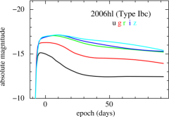
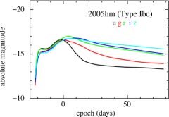
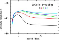
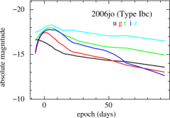
Figure 1.— Absolute magnitude light curves of SN Ib/c discovered and observed by SDSS-II, which are part of the template library – SN 2005hl (top left), SN 2005hm (top right), SN 2006fo (bottom left), and SN 2006jo (bottom right). [See online version for color figures.]

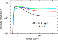
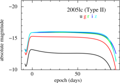
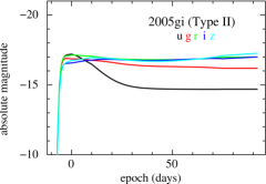
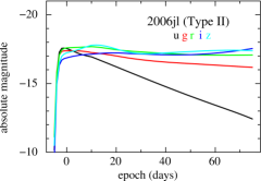
Figure 2.— Absolute magnitude light curves of SN II discovered and observed by SDSS-II, which are part of the template library – SN 2004hx (top left), SN 2005lc (top right), SN 2005gi (bottom left), and SN 2006jl (bottom right). [See online version for color figures.]

First, in addition to finding the light curve model with the minimum $\chi^{2}_{r}$ through a grid search, the software computes the Bayesian probabilities that a candidate could be a Type Ia, Type Ib/c, or a Type II SN. The algorithm is similar to that of Poznanski et al. (2007a) except that we subclassify CC SN into Types Ib/c and II using an extended set of templates (see below), and also allow the SN Ia light curve shape parameter and distance modulus to vary in the fits. Specifically, we calculate the Bayesian Evidence $E$ by marginalizing the product of the likelihood function and prior probabilities over the model parameter space. For the SN Ia models, there are five model parameters – redshift $z$, $V$-band host galaxy extinction $A_{V}$, time of maximum light $T_{\mathrm{max}}$, $\Delta m_{15}(B)$ (Phillips, 1993; Phillips et al., 1999), and distance modulus $\mu$. Milky Way extinction is modeled assuming the Cardelli, Clayton, & Mathis (1989) law with $R_{V}=3.1$, while extinction in the SN host galaxy assumes a total-to-selective extinction ratio of $R_{V}\equiv A_{V}/E(B-V)=2.2$ (Kessler et al., 2009a). Priors in $A_{V}$, $T_{\mathrm{max}}$, and $\mu$ can also be applied optionally, but we set them to be flat in this present work. For the redshift, we evaluate each light curve twice using 1) a flat prior and 2) a gaussian prior if an external redshift estimate $z_{\mathrm{ext}}$ and uncertainty $\sigma_{z}$ are available from either the host galaxy (photometric or spectroscopic redshift) or the SN spectrum. The SN Ia Bayesian evidence is therefore,

$$E_{\mathrm{Ia}}=\int_{\mathrm{all~{}parameters}}P(z)~{}e^{-\chi^{2}/2}~{}dz~{}dA_{V}~{}dT_{\mathrm{max}}~{}d\Delta m_{15,B}~{}d\mu,$$ (1)

where,

$$P(z)=\frac{1}{\sqrt{2\pi\sigma_{z}}}~{}e^{-(z-z_{\mathrm{ext}})^{2}/2\sigma_{z}^{2}}.$$ (2)

When an external redshift is not available, we assume the prior to be flat by setting $P(z)=1$. For the SN Ib/c and SN II models, the integral over $\Delta m_{15}(B)$ is replaced with a summation over the individual templates used in the comparison,

$$E_{\mathrm{Ibc,II}}=\sum_{\mathrm{templates}}\int P(z)~{}e^{-\chi^{2}/2}~{}dz~{}dA_{V}~{}dT_{\mathrm{max}}~{}d\mu.$$ (3)

The Bayesian probability of one of the three possible SN types is then given by,

$$P_{\mathrm{type}}=\frac{E_{\mathrm{type}}}{E_{\mathrm{Ia}}+E_{\mathrm{Ibc}}+E_{\mathrm{II}}}.$$ (4)

The probabilities $P_{\mathrm{type}}$ and minimum $\chi^{2}_{r}$ values calculated using the gaussian spectroscopic redshift prior are denoted with a subscript $z$ (i.e., $P_{\mathrm{z,type}}$ and $\chi^{2}_{z,r}$). External photometric redshifts of the host galaxies are not used in the fits in this work. The probabilities are normalized such that,

$$P_{\mathrm{Ia}}+P_{\mathrm{Ibc}}+P_{\mathrm{II}}=1,$$ (5)

which is equivalent to assuming that the SN candidate is a real SN and not another class of variable sources. This assumption is reasonable, since sources in Stripe 82 with a prior history of variability and other multi-year variables are rejected from our analysis (Sako et al., 2008). This set of Bayesian probabilities is useful because it quantifies the relative likelihood of SN types – the best-fit minimum $\chi^{2}_{r}$ alone is not a good indicator of the most likey SN type. As advocated by Kuznetsova & Connolly (2007), we therefore select SN Ia based on both the Bayesian probability $P_{\mathrm{Ia}}$ and the goodness-of-fit $\chi^{2}_{r}$.

Next, although the SN Ia light curve models used herein are the same as those described in Sako et al. (2008), we have assigned empirical model errors that yield reasonable $\chi^{2}_{r}$ values for light curves with high S/N ratio. The assumed magnitude errors $\delta m$ on the $gri$ model light curves depend on the rest-frame epoch $t$ in days from $B$-band maximum as follows,

$$\delta m_{\rm{Ia}}=\left\{\begin{array}[]{ll}0.08+0.04\times(|t|/20)&|t|<20~{}\mathrm{days},\\ 0.12+0.08\times((|t|-20)/60)&|t|\geq 20~{}\mathrm{days}.\end{array}\right.$$ (6)

The CC SN light curve templates have error in $gri$ given by,

$$\delta m_{\rm{CC}}=0.08+0.08\times(|t|/60)$$ (7)

for all epoch. The model errors in $u$ and $z$ are chosen to be twice the above values due to larger intrinsic model variations and calibration uncertainties in these bands. These $\delta m$ parameters were determined to provide reasonable $\chi^{2}_{r}$ values ($\chi^{2}_{r}$ $\sim 1$) primarily for nearby SN candidates with small photometric errors. They do not affect the fit results of faint candidates.

Third, we adopt CC SN light curve templates from a sample of nearby SN discovered and observed by SDSS-II. Specifically, we use four SN Ib/c templates and four SN II templates as listed in Table 1. The SDSS-II CC SN light curve templates were generated using the Nugent, Kim, & Perlmutter (2002) spectral templates, interpolating between epochs, and warping them to match each of the observed ugriz light curves at their respective spectroscopic redshifts. For all SN Ib/c, we use Nugent’s normal Ibc spectral templates, and we use the Type II-P templates for all SN II. The SN II light curve photometry are available from D’Andrea et al. (2010).

The set of eight core-collapse templates listed in Table 1 were selected from a larger group of 24 templates (5 Nugent, 11 SDSS-II, and 8 from the SUSPECT database) by empirically maximizing the purity of the confirmed SN Ia sample. Core-collapse templates that either frequently misidentify SN Ia as CC SN or correctly identify only a small number of confirmed CC SN were excluded. Rare, peculiar SN Ia are also excluded from our template library. We also do not include templates for other types of variable sources, most notably the active galactic nuclei (AGN), since there are other ways of rejecting the majority of these events. The rest-frame absolute magnitude ugriz light curves of the eight CC SN used as templates in this analysis are shown in Figures 1 and 2.

Finally, while the Bayesian classification probabilities are computed through marginalization over the grid of the model parameters, the posterior probability distributions for each of the five parameters are estimated by running a Markov Chain Monte Carlo (MCMC). This results in a significant reduction of computing time and more reliable estimates of the parameter uncertainties, since the probability distributions are often asymmetric, show significant correlations, and can often have more than one local maximum. It is also straightforward to incorporate additional model parameters and priors.

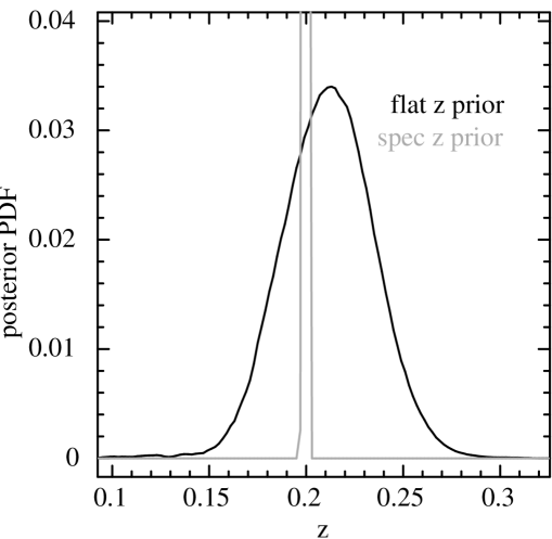
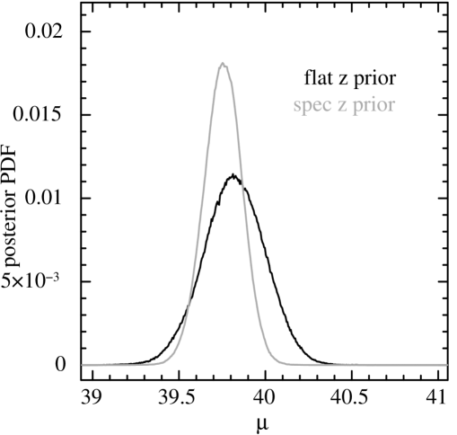
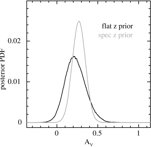
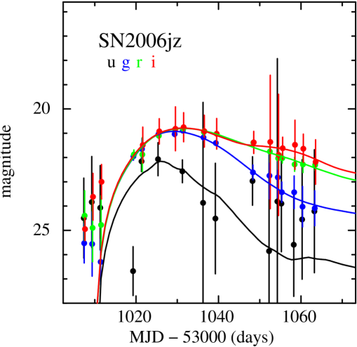
Figure 3.— An example of the posterior probability distribution functions (PDF) for a spectroscopically-confirmed SN Ia 2006jz at $z=0.20$. The observed $ugri$ light curves and the best-fit SN Ia model are shown on the bottom right panel. The top-left and middle-left panels show 1- and 2-$\sigma$ contours in the $z$-$\mu$ and $z$-$A_{V}$ planes, respectively, assuming a flat redshift prior. The $\times$ indicates the median parameter values when a spectroscopic-redshift prior is used. The two panels on the right and the bottom-left panel show the posterior PDF in $\mu$, $A_{V}$, and $z$ marginalized over the other 4 parameters using the flat (black) and spectroscopic (gray) redshift priors.

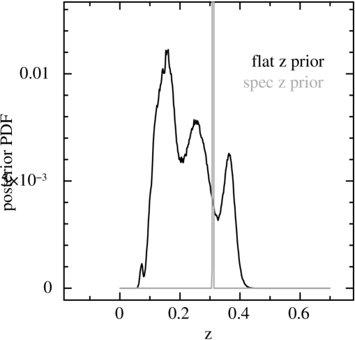
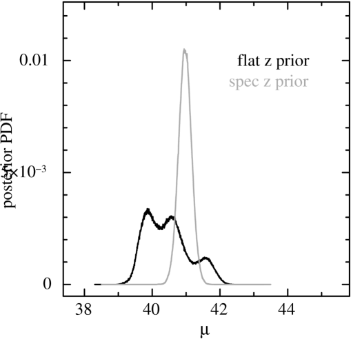
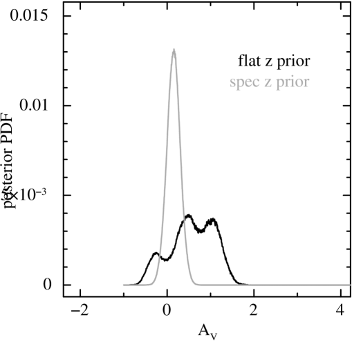
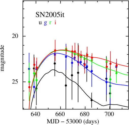
Figure 4.— Same as in Figure 3 for a spectroscopically-confirmed SN Ia 2005it at $z=0.30$.

Figure 3 shows an example output from PSNID for a spectroscopically-confirmed SN Ia, 2006jz at $z=0.20$. Derived parameter constraints from the MCMC are shown for both the flat and spectroscopic redshift priors. There are two general points that are worth noting. First, $z$ and $A_{V}$ are anti-correlated in the sense that a low-$z$, high-$A_{V}$ SN Ia is similar to a high-$z$, low-$A_{V}$ event. This is expected, since redshift and dust both have the effect of reddening the light curves. But since dust also attenuates the light, a larger $A_{V}$ value must be compensated for by putting the event at a smaller distance modulus. This happens in the way such that $z$ and $\mu$, marginalized over the other three parameters, are positively correlated. The slope of this correlation is redshift-dependent. Second, the widths of the marginalized $\mu$ and $A_{V}$ probability distribution function (PDF) for the flat redshift prior are only a factor $\sim 2$ larger than those for a spectroscopic redshift prior. This general behavior is true for most of our well-observed SN Ia, although the constraints using a flat-$z$ prior degrades dramatically at higher redshifts, as shown in Figure 4 for a $z=0.30$ confirmed SN Ia 2005it.

2.2. Confirmed and Unconfirmed Samples

We first divide the full sample of SN candidates into two groups – the spectroscopically confirmed and unconfirmed samples. The unconfirmed sample consists of sources of unknown type with no spectroscopy of the active SN candidate, but a subset of the events do have spectroscopy of their host galaxies. The spectroscopically-confirmed sample consists of SN Ia, SN Ib/c, SN II, as well as variable AGN. This sample is used to study the classification criteria and also allows us to estimate the selection efficiency and purity, which is a crucial part of our analysis. The $ugriz$ multi-band light curves of all SN candidates are constructed using the Scene-Modeling Photometry method (smp; Holtzman et al., 2008) and analyzed using the PSNID software described above.

The full SN sample is analyzed with PSNID, and we select the candidates that have light curve coverage and signal-to-noise (S/N) ratio that are appropriate for photometric SN Ia classification. Specifically, we consider only the candidates that meet the following three criteria: (1) Have at least one epoch of photometry near peak at $-5<t<+5$ days in the SN rest frame and at least one additional epoch after peak at $t>+15$ days, which are determined from to the best-fit SN Ia model, irrespective of whether or not the fit is acceptable; (2) Have maximum S/N ratio greater than five in at least two of the $gri$ bands, and; (3) Were detected during only one search season. These cuts are referred to as the light curve quality cuts.

The spectroscopically-confirmed sample consists of 508 SN Ia, 80 CC SN (18 SN Ib/c, 62 SN II), and 202 AGN. We refer to these as the “conf-Ia”, “conf-CC”, and the “conf-AGN” samples. After imposing the light curve quality cuts, this sample is reduced to 367 SN Ia, 45 CC SN, and 83 AGN, for a total of 495 events when a flat spectroscopic redshift prior is used. Using the spectroscopic redshift prior results in 551 events. The numbers differ since the two forms of the redshift priors can result in best-fit SN Ia models with dramatically different dates of maximum light, especially for the AGN.

There is a significant bias in the spectroscopically-confirmed SN sample toward brighter events. For the SDSS-II SN Survey, our primary goal was to discover and study the properties of SN Ia, so only a small fraction of CC SN candidates were observed for spectroscopy. A detailed study of the impact on photometric SN Ia typing due to contaminating sources is, therefore, limited by this small number of spectroscopically confirmed CC SN.

To help quantify this bias, we identified the SN candidates that are associated with galaxies with spectra from the SDSS spectroscopic survey (Eisenstein et al., 2001; Strauss et al., 2002; Richards et al., 2002). These galaxies have well-defined selection criteria and, as we describe below, will help quantify the spectroscopic targeting bias and to obtain a better estimate of the level of contamination from non-SN Ia events. There are a total of 2369 SN candidates that are within $10\arcsec$ from an SDSS spectroscopic galaxy. This sample is referred to as the “$z_{\mathrm{SDSS}}$” sample. After light curve quality cuts, there are 448 and 499 sources for the flat and spectroscopic redshift priors, respectively, which includes both confirmed and unconfirmed SN candidates. The majority of the sources are rejected because of their multi-year variability, suggesting that these sources are likely variable AGN whose nuclear activity is not immediately apparent from their optical spectra. The samples are summarized in Table 2. The redshift distributions of the four different spectroscopic samples are shown in Figure 5.

Table 2The SDSS-II Spectroscopic Sample

		Flat Redshift Prior			Spectroscopic Redshift Prior
Type	Total	Good	$P_{\mathrm{Ia}}$ $\geq 0.9$	$P_{\mathrm{Ia}}$ $\leq 0.1$	Good	$P_{\mathrm{Ia}}$ $\geq 0.9$	$P_{\mathrm{Ia}}$ $\leq 0.1$
Confirmed SN Ia	508	367	357	2	371	366	1
Confirmed CC SN	80	45	14	30	45	11	32
Confirmed AGN	202	83	32	44	135	86	46
SN with $z_{\rm{SDSS}}$	2369	448	248	159	499	317	150
Total	3159	732	539	201	788	599	163

Figure 5.— The redshift distributions of the conf-Ia (top left), conf-CC (top right), conf-AGN (bottom left), and $z_{\mathrm{SDSS}}$ (bottom right) samples used in our studies (see § 2.2 for descriptions). The solid and dashed histograms represent the samples that pass our light curve quality cuts with the flat and spectroscopic redshift priors, respectively. The redshift bins are $\Delta z=0.05$ wide.

The unconfirmed sample consists of a total of 3221 candidates that pass the same light curve quality cuts. Of these 3221 candidates, 2776 have no spectroscopic observations, while the remaining 445 candidates are either part of the $z_{\mathrm{SDSS}}$ sample described above (230 candidates) or have host galaxy redshifts from our own follow-up observations (215 candidates).

A histogram of the maximum $r$-band S/N of this sample is shown in Figure 6. The mean S/N of $\sim 30$ for the spectroscopic sample is substantially higher than that of the photometric sample, which has a mean S/N of $\sim 10$. The implications of this difference are discussed in § 8.

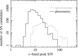
Figure 6.— The distributions of maximum $r$-band signal-to-noise ratio (S/N) of the spectroscopically-confirmed SN candidates (dashed) and photometric candidates (solid) considered in this work. The spectroscopic sample has an average peak S/N of $\sim 30$ while the photometric sample has average S/N of $\sim 10$.

3. SN Classification Figure of Merit

Since our goal here is to identify SN Ia, we define the photometric typing efficiency $\epsilon_{\rm{Ia}}$ as the fraction of SN Ia, after software S/N light curve quality cuts, that are photometrically identified as SN Ia. Letting $\mathcal{N}_{\rm{Ia}}^{\rm{true}}$ be the number of true SN Ia photometrically identified as SN Ia and $\mathcal{N}_{\rm{Ia}}^{\rm{CUT}}$ be the total number of SN Ia in the sample after the light curve quality cuts, we define the photometric SN Ia selection efficiency to be,

$$\epsilon_{\rm{Ia}}=\frac{\mathcal{N}_{\rm{Ia}}^{\rm{true}}}{\mathcal{N}_{\rm{Ia}}^{\rm{CUT}}}.$$ (8)

Note that this is not the true SN Ia identification efficiency since the denominator $\mathcal{N}_{\rm{Ia}}^{\rm{CUT}}$ includes only the events that pass the S/N and light curve quality cuts. In terms of the total number of SN Ia ($\mathcal{N}_{\rm{Ia}}^{\rm{TOT}}$) that were detected in the area observed by the survey,

$$\mathcal{N}_{\rm{Ia}}^{\rm{CUT}}=\epsilon_{\rm{CUT}}\mathcal{N}_{\rm{Ia}}^{\rm{TOT}}$$ (9)

where $\epsilon_{\rm{CUT}}$ is, in general, a function of $z$, $A_{V}$, $\Delta m_{15}(B)$, peak magnitude, time of maximum light, software detection threshold, requirements on light curve S/N and temporal coverage, as well as the observing conditions. The determination of the value of $\epsilon_{\rm{CUT}}$ is beyond the scope of the paper, but the effect of our selection cuts can be modeled using the SNANA Package.

Adopting the convention similar to that used in evaluating the SN Photometric Classification Challenge (hereafter SNPhotCC; K10b) we define the photometric purity $\eta_{\rm{Ia}}$ as the fraction of the candidates identified as SN Ia that are actual SN Ia with a penalty factor $\mathcal{W}_{\rm{Ia}}^{\rm{false}}$ described below. Letting $\mathcal{N}_{\rm{Ia}}^{\rm{false}}$ be the number of non-SN Ia incorrectly identified as SN Ia, the photometric purity of the sample is,

$$\eta_{\rm{Ia}}=\frac{\mathcal{N}_{\rm{Ia}}^{\rm{true}}}{\mathcal{N}_{\rm{Ia}}^{\rm{true}}+\sum_{i}\mathcal{W}_{\rm{Ia},i}^{\rm{false}}\mathcal{N}_{\rm{Ia},i}^{\rm{false}}},$$ (10)

where the sum in the denominator allows for several classes $i$ of contaminating sources (e.g., CC SN, AGN, and variable stars) possibly with different penalty factors. We define a figure of merit ($\mathcal{C}_{\rm{FoM-Ia}}$) as,

$$\mathcal{C}_{\rm{FoM-Ia}}=\epsilon_{\rm{Ia}}\times\eta_{\rm{Ia}}.$$ (11)

This definition of $\mathcal{C}_{\rm{FoM-Ia}}$ is designed for real data and differs from the pseudo-purity from the SNPhotCC by the unknown factor $1/\epsilon_{\rm{CUT}}$, i.e., $\mathcal{C}_{\rm{FoM-Ia}}=\mathcal{C}_{\rm{FoM-Ia}}^{\rm{SNPhotCC}}/\epsilon_{\rm{CUT}}$. K10b also define the true purity to be the case for $\mathcal{W}_{\rm{Ia}}^{\rm{false}}=1$. This figure of merit is only one measure of success, and it is not necessarily the optimal measure for all types of studies. Higher SN Ia purity might be more important than efficiency for certain studies, and vice versa. Finally, we define the contamination $\kappa_{\rm{Ia}}$ as,

$$\kappa_{\rm{Ia}}=1-\eta_{\rm{Ia}}.$$ (12)

These quantities determined with the spectroscopic redshift prior are designated with a subscript $z$.

To give a simple numerical example, consider a survey that is capable of detecting 100 SN Ia that pass S/N and light curve quality cuts. A photometric classifier that identifies 90 candidates as SN Ia, of which 10 are actually non-Ia events has an efficiency of $\epsilon_{\rm{Ia}}=80/100=0.80$, purity of $\eta_{\rm{Ia}}=80/90=0.89$, and contamination of $\kappa_{\rm{Ia}}=1-0.89=0.11$. In practice, however, these quantities can be determined only for the spectroscopically confirmed SN sample for which the correct type is known. The efficiency, purity, or some combination of these two parameters can be optimized by choosing the appropriate values for $P_{\mathrm{Ia}}$ and $\chi^{2}_{r}$. If the spectroscopic sample is an unbiased representation of all of the SN candidates, then one can expect the efficiency and the purity of both the spectroscopic and photometric samples to be the same within statistical uncertainties. However, this is almost never the case in a blind SN survey given limited spectroscopic resources. SN candidates that are brighter and/or suffer less host galaxy contamination will have higher spectroscopic success and completeness. This is illustrated in Figure 6, which shows that the light curve peak S/N of the spectroscopic sample is on average a factor of $\sim 3$ higher than that of the photometric sample. Below we describe a method to correct for this bias and to estimate the efficiency and purity of the photometric sample using a limited and biased spectroscopic training set.

4. Estimating the Efficiency and Purity

4.1. SN Ia Identification With Spectroscopic Redshifts

Figure 7.— The distribution of $P_{z,{\mathrm{Ia}}}$ and $\chi^{2}_{z,r}$ values for the spectroscopically-confirmed SN Ia (top panel) and CC SN. Spectroscopic redshifts are used as priors in all of the fits.

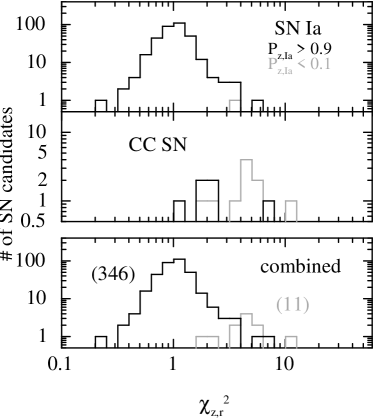
Figure 8.— Histograms of best-fit $\chi^{2}_{z,r}$ values for a SN Ia model for $P_{\mathrm{Ia}}\geq 0.9$ (black) and $P_{\mathrm{Ia}}\leq 0.1$ (gray) for the spectroscopically confirmed SN Ia (top panel) and CC SN (bottom panel).

We first estimate the efficiency and purity of photometric SN Ia identification when spectroscopic redshifts are used as priors in the light curve fits. We determine $\mathcal{N}_{\rm{z,Ia}}^{\rm{true}}$ and $\mathcal{N}_{\rm{z,Ia}}^{\rm{false}}$ from the spectroscopic SN Ia and CC SN and how they depend on the minimum $P_{z,{\mathrm{Ia}}}$ and the maximum allowed $\chi^{2}_{z,r}$. This is relevant for future SN surveys that will, for example, obtain spectra of all SN candidate host galaxies after the search, but not spectra of all the active SN candidates. The values for $P_{z,{\mathrm{Ia}}}$ and $\chi^{2}_{z,r}$ are shown in Figure 7 separately for the spectroscopically confirmed SN Ia and CC SN samples.

As shown in the top panel of Figure 7, all but a handful of SN Ia are well fit to a SN Ia model. Of the $\mathcal{N}_{\rm{z,Ia}}^{\rm{CUT}}=371$ spectroscopic SN Ia that pass the light curve quality cuts, 366 sources have $P_{z,{\mathrm{Ia}}}$ $\geq 0.9$. Only a single SN Ia (SN 2007qd; McClelland et al. 2010) has $P_{z,{\mathrm{Ia}}}$ $\leq 0.1$. This event is a nearby peculiar 2002cx-like event, which is underluminous compared to normal SN Ia and has an extremely low expansion velocity (Li et al., 2003; Jha et al., 2006b). There are other nearby peculiar SN Ia in our sample (SN 2005hk Phillips et al. 2007, SN 2005gj Aldering et al. 2006; Prieto et al. 2007), but these candidates were detected over two search seasons due to their brightness and slow decline, and were, therefore, rejected. The bottom panel of the same figure, however, shows that a substantial fraction of the spectroscopic CC SN also satisfy $P_{z,{\mathrm{Ia}}}$ $\geq 0.9$ implying that the contamination can be significant depending on the maximum allowed $\chi^{2}_{z,r}$ value used for the SN Ia identification. Specifically, 11 out of the 45 CC SN (24%) that satisfy our light curve quality cuts have $P_{z,{\mathrm{Ia}}}$ $\geq 0.9$. If no other cuts are invoked, then $\mathcal{N}_{\rm{z,Ia}}^{\rm{true}}=366$ and $\mathcal{N}_{\rm{z,Ia}}^{\rm{false}}=11$. We also note that the majority of the sources have either $P_{z,{\mathrm{Ia}}}$ $\sim 0$ or $P_{z,{\mathrm{Ia}}}$ $\sim 1$, so both $\mathcal{N}_{\rm{z,Ia}}^{\rm{true}}$ and $\mathcal{N}_{\rm{z,Ia}}^{\rm{false}}$ are not sensitive to the precise choice of the minimum $P_{z,{\mathrm{Ia}}}$.

Before determining how $\mathcal{N}_{\rm{z,Ia}}^{\rm{true}}$ and $\mathcal{N}_{\rm{z,Ia}}^{\rm{false}}$ depend on the choice of the maximum $\chi^{2}_{z,r}$, we note that 5 of the 11 CC SN with $P_{z,{\mathrm{Ia}}}$ $\geq 0.9$ can be rejected by requiring the light curve photo-$z$ ($z_{\mathrm{lc}}$), using a flat redshift prior, to be within $3\sigma$ of the spectroscopic redshift $z_{\mathrm{spec}}$; i.e., $|$$z_{\mathrm{lc}}$ – $z_{\mathrm{spec}}$$|$/$\sigma_{z}<3$. We reject candidates that fail this cut, and show the distributions of the $\chi^{2}_{z,r}$ values for the SN Ia and CC SN in Figure 8 for $P_{z,{\mathrm{Ia}}}$ $\geq 0.9$ and $P_{z,{\mathrm{Ia}}}$ $\leq 0.1$. Of the 366 SN Ia and 11 CC SN with good light curves and $P_{z,{\mathrm{Ia}}}$ $\geq 0.9$, 22 and 5 candidates, respectively, are rejected by this requirement on redshift agreement. Therefore, there are only 6 CC SN that satisfy all SN Ia selection cuts.

In the last step, we estimate the unknown factor $\mathcal{W}_{\rm{z,Ia}}^{\rm{false}}$, which can be interpreted as a penalty factor for spectroscopic incompleteness and targeting biases. The SDSS-II SN Survey follow-up strategy was to observe the “good” SN Ia candidates at higher priority than the CC SN candidates, especially for the fainter ($r\gtrsim 20.5$ mag) sources due to limited spectroscopic resources. A simple interpretation of this factor is that if our follow-up strategy had instead been to observe a random sample of SN candidates, then we would have spectroscopically identified $\mathcal{W}_{\rm{z,Ia}}^{\rm{false}}$ times more CC SN.

One way to estimate this bias factor is to select a subsample of SN candidates with spectroscopic redshifts, which is representative of the underlying distribution of the SN types. The ratio of these candidates with $P_{z,{\mathrm{Ia}}}$ $\leq 0.1$ to those with $P_{z,{\mathrm{Ia}}}$ $\geq 0.9$ can then be interpreted to be approximately the ratio of CC SN to SN Ia in our survey.

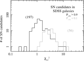
Figure 9.— Histograms of best-fit $\chi^{2}_{r}$ values for a SN Ia model for $P_{\mathrm{z,Ia}}\geq 0.9$ (black) and $P_{\mathrm{z,Ia}}\leq 0.1$ (gray) for the SN candidates in SDSS spectroscopic galaxies using the redshift as a prior.

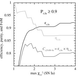
Figure 10.— The efficiency, purity, and figure of merit for the spectroscopically-confirmed SN as functions of the maximum-allowed $\chi^{2}_{z,r}$ for $P_{z,{\mathrm{Ia}}}$ $\geq 0.9$.

Figure 11.— The distributions of $P_{\mathrm{Ia}}$ and $\chi^{2}_{r}$ values for the spectroscopically confirmed SN Ia (top panel), CC SN (middle panel), and AGN (bottom panel). The fits were performed with a flat redshift prior.

This can be done by considering the SN candidates in galaxies with redshifts from the SDSS spectroscopic survey, which has a set of well-defined selection criteria. We identify candidates in the main galaxy (Strauss et al., 2002), quasar (Richards et al., 2002), and the Luminous Red Galaxy (LRG; Eisenstein et al. 2001) samples. The LRG sample is several magnitudes deeper than the main galaxy sample and consists primarily of passive galaxies with old stellar populations, which do not host any CC SN. We include this sample to account for the fact that SN Ia are also on average a few magnitudes more luminous than CC SN, so a magnitude-limited survey will discover many more SN Ia than CC SN. The distributions of $\chi^{2}_{z,r}$ for $P_{z,{\mathrm{Ia}}}$ $\geq 0.9$ and $P_{z,{\mathrm{Ia}}}$ $\leq 0.1$ for candidates in the SDSS galaxy spectroscopy sample with $|$$z_{\mathrm{lc}}$ – $z_{\mathrm{spec}}$$|$/$\sigma_{z}<3$ are shown in Figure 9. The ratio of the number of candidates with $P_{z,{\mathrm{Ia}}}$ $\geq 0.9$ to those with $P_{z,{\mathrm{Ia}}}$ $\leq 0.1$ is $197/56=3.5$ compared to $350/11=32$ for the combined spectroscopic sample shown in the bottom panel of Figure 8. The bias (penalty) factor for the spectroscopic sample can, therefore, be estimated to be $\mathcal{W}_{\rm{z,Ia}}^{\rm{false}}=32/3.5=9.0$. An unbiased spectroscopic follow-up strategy would have resulted in $\mathcal{W}_{\rm{z,Ia}}^{\rm{false}}=9.0$ times more contaminating CC SN for SN Ia identification.

We use this penalty factor to calculate $\epsilon_{\rm{z,Ia}}$ and $\eta_{\rm{z,Ia}}$ as functions of the maximum $\chi^{2}_{z,r}$. The expression for the purity is,

$$\eta_{\rm{z,Ia}}=\frac{\mathcal{N}_{\rm{z,Ia}}^{\rm{true}}}{\mathcal{N}_{\rm{z,Ia}}^{\rm{true}}+\mathcal{W}_{\rm{z,Ia}}^{\rm{false}}\mathcal{N}_{\rm{z,Ia}}^{\rm{false}}}.$$ (13)

Figure 10 shows how $\epsilon_{\rm{z,Ia}}$, $\eta_{\rm{z,Ia}}$, and $\mathcal{C}_{\rm{z,FoM-Ia}}$ depend on the maximum-allowed $\chi^{2}_{z,r}$ for $P_{z,{\mathrm{Ia}}}$ $\geq 0.9$. The figure of merit has a broad maximum value of $\mathcal{C}_{\rm{z,FoM-Ia}}\sim 0.84$ at approximately $\chi^{2}_{z,r}$ $=1.8$, where the efficiency and purity are $\sim 89$% and $\sim 94$%, respectively. A caveat to the estimate of $\eta_{\rm{z,Ia}}$ is that it is based on only six confirmed CC SN that pass our SN Ia selection cuts.

4.2. SN Ia Identification without Spectroscopic Redshifts

We next determine $\mathcal{N}_{\rm{Ia}}^{\rm{true}}$ and $\mathcal{N}_{\rm{Ia}}^{\rm{false}}$ when no external redshift information is available to provide additional constraints in the light curve fits. Here we have an additional source of contaminating sources – variable AGN – which can be identified if either the galaxy spectrum is available or the candidate is variable over a long period of time ($\gtrsim 1$ year). We use the confirmed SN and the AGN samples discussed in § 2.2 to determine how the efficiency, purity, and figure of merit depend on the minimum $P_{\mathrm{Ia}}$ and the maximum allowed $\chi^{2}_{r}$ using the flat redshift prior. The three panels in Figure 11 show the $P_{\mathrm{Ia}}$ and $\chi^{2}_{r}$ values for the spectroscopic SN Ia, CC SN, and AGN samples. As with the previous case, most of the spectroscopic SN Ia are clustered near $P_{\mathrm{Ia}}$ $\sim 1$ and $\chi^{2}_{r}$ $\sim 1$ indicating that they are well-fit to SN Ia models. There are also a handful of CC SN and AGN with $P_{\mathrm{Ia}}$ $\sim 1$, however, so the amount of contamination can again be substantial depending on the maximum allowed $\chi^{2}_{r}$.

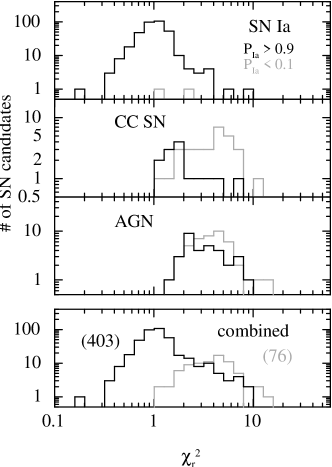
Figure 12.— Histograms of best-fit $\chi^{2}_{r}$ values for a SN Ia model for $P_{\mathrm{Ia}}$ $\geq 0.9$ (black) and $P_{\mathrm{Ia}}$ $\leq 0.1$ (gray) for the spectroscopically confirmed (from top to bottom) 1) SN Ia, 2) CC SN, 3) AGN, and 4) all three samples combined. Note that the vast majority of SN Ia have $P_{\mathrm{Ia}}$ $\geq 0.9$. The contaminating false-positives are the CC SN and AGN represented by the black histograms with $P_{\mathrm{Ia}}\geq 0.9$, and there are only a small number of those sources in our sample.

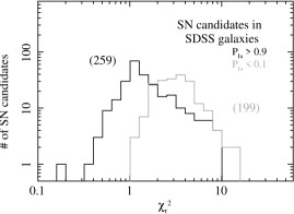
Figure 13.— Histograms of best-fit $\chi^{2}_{r}$ values for a SN Ia model for $P_{\mathrm{Ia}}\geq 0.9$ (black) and $P_{\mathrm{Ia}}\leq 0.1$ (gray) for the SN candidates in SDSS spectroscopic galaxies.

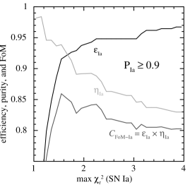
Figure 14.— The efficiency, purity, and figure of merit for the spectroscopically-confirmed SN as functions of the maximum-allowed $\chi^{2}_{r}$ for $P_{\mathrm{Ia}}$ $\geq 0.9$.

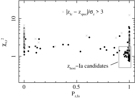
Figure 15.— $P_{z,{\mathrm{Ia}}}$ vs $\chi^{2}_{z,r}$ for the 445 photometric candidates with galaxy spectroscopic redshifts. Candidates that do not meet the light curve photo-$z$ cut ($|$$z_{\mathrm{lc}}$ – $z_{\mathrm{spec}}$$|$/$\sigma_{z}<3$) are shown as crosses. The 210 $z_{\mathrm{host}}$-Ia candidates identified are bounded by the red box shown in the lower right.

We also show in Figure 12 histograms of the $\chi^{2}_{r}$ values for the same sources for $P_{\mathrm{Ia}}$ $\geq 0.9$. Of the $\mathcal{N}_{\rm{Ia}}^{\rm{CUT}}=367$ spectroscopic SN Ia that pass our light curve quality cuts, 357 sources have $P_{\mathrm{Ia}}$ $\geq 0.9$. There are also 14 CC SN and 32 AGN with $P_{\mathrm{Ia}}$ $\geq 0.9$.

For estimating $\eta_{\rm{Ia}}$, we apply the penalty factor only on the CC SN sample where the bias is more significant. Almost all of the spectroscopic AGN confirmation came from SDSS quasar spectroscopy (Richards et al., 2002) and not from our own targeting, so we assume that this sample is unbiased. The expression for the efficiency is given in Eq.8. We write the purity explicitly as,

$$\eta_{\rm{Ia}}=\frac{\mathcal{N}_{\rm{Ia}}^{\rm{true}}}{\mathcal{N}_{\rm{Ia}}^{\rm{true}}+\mathcal{W}_{\rm{Ia,CC}}^{\rm{false}}\mathcal{N}_{\rm{Ia,CC}}^{\rm{false}}+\mathcal{N}_{\rm{Ia,AGN}}^{\rm{false}}},$$ (14)

where we have assumed $\mathcal{W}_{\rm{Ia,AGN}}^{\rm{false}}=1$. The penalty factor $\mathcal{W}_{\rm{Ia,CC}}^{\rm{false}}$ can be estimated from the histograms shown in the bottom panel of Figure 12 and Figure 13. Specifically, we have $\mathcal{W}_{\rm{Ia,CC}}^{\rm{false}}=(403/76)/(259/199)=4.1$ using the same method as for the case with the spectroscopic redshift prior. We show in Figure 14 the efficiency and purity as a function of the maximum-allowed $\chi^{2}_{r}$ value. Also shown is the figure of merit, which exhibits a broad maximum at $\mathcal{C}_{\rm{FoM-Ia}}=0.86$. At $\chi^{2}_{r}$ $\sim 1.6$, the efficiency and purity are $\sim 92$% and $\sim 94$%, respectively.

5. SDSS-II Photometric SN Ia Candidates

Table 3SDSS-II $z_{\mathrm{host}}$-Ia Candidates

SDSS ID	RA	Dec	$z_{\mathrm{spec}}$	$A_{V}$	$\Delta m_{15}(B)$	$P_{z,{\mathrm{Ia}}}$	$\chi^{2}_{z,r}$
703	$-23.782080$	$+0.650725$	$0.3000\pm 0.0100$	$0.04^{+0.16}_{-0.18}$	$0.70^{+0.13}_{-0.08}$	1.000	0.99
779	$26.673738$	$-1.020580$	$0.2377\pm 0.0005$	$0.21^{+0.13}_{-0.13}$	$0.85^{+0.10}_{-0.09}$	1.000	0.80
841	$48.495991$	$-1.010015$	$0.2991\pm 0.0005$	$-0.17^{+0.16}_{-0.18}$	$1.02^{+0.20}_{-0.16}$	1.000	0.99
1415	$6.106480$	$+0.599307$	$0.2119\pm 0.0002$	$0.66^{+0.13}_{-0.13}$	$0.76^{+0.09}_{-0.08}$	1.000	0.93
1461	$24.372675$	$+0.209735$	$0.3407\pm 0.0005$	$0.33^{+0.11}_{-0.11}$	$1.08^{+0.12}_{-0.12}$	1.000	1.07
1595	$-38.432114$	$-0.554060$	$0.2136\pm 0.0005$	$0.07^{+0.09}_{-0.09}$	$1.03^{+0.08}_{-0.08}$	1.000	1.56
1748	$-6.887835$	$-0.482495$	$0.3397\pm 0.0001$	$0.52^{+0.20}_{-0.19}$	$0.83^{+0.16}_{-0.13}$	0.996	1.00
1775	$-41.006622$	$-1.009430$	$0.3050\pm 0.0100$	$-0.27^{+0.17}_{-0.17}$	$1.26^{+0.15}_{-0.15}$	1.000	1.07
1835	$-47.335869$	$+1.071860$	$0.2716\pm 0.0100$	$-0.19^{+0.19}_{-0.19}$	$1.28^{+0.22}_{-0.20}$	1.000	1.31
$\cdots$

Table 4SDSS-II Photo-Ia Candidates

SDSS ID	RA	Dec	$z_{\mathrm{lc}}$	$A_{V}$	$\Delta m_{15}(B)$	$P_{\mathrm{Ia}}$	$\chi^{2}_{r}$
822	$40.560776$	$-0.862157$	$0.167^{+0.065}_{-0.050}$	$0.51^{+0.40}_{-0.47}$	$1.24^{+0.14}_{-0.14}$	1.000	1.38
859	$-9.448275$	$+0.386555$	$0.305^{+0.025}_{-0.036}$	$0.04^{+0.28}_{-0.31}$	$0.77^{+0.13}_{-0.09}$	1.000	1.25
904	$21.095400$	$-0.124883$	$0.288^{+0.029}_{-0.026}$	$-0.26^{+0.28}_{-0.34}$	$1.10^{+0.22}_{-0.17}$	0.999	1.00
1158	$17.275431$	$-0.352185$	$0.694^{+0.006}_{-0.063}$	$-0.58^{+0.50}_{-0.31}$	$1.55^{+0.19}_{-0.29}$	1.000	1.01
1243	$-18.340113$	$-0.764753$	$0.188^{+0.100}_{-0.102}$	$0.89^{+0.73}_{-0.67}$	$0.69^{+0.09}_{-0.06}$	1.000	1.47
1285	$-38.216843$	$+0.543195$	$0.345^{+0.049}_{-0.078}$	$0.21^{+0.47}_{-0.38}$	$1.06^{+0.25}_{-0.20}$	1.000	1.01
1302	$53.654808$	$+0.891903$	$0.282^{+0.039}_{-0.042}$	$-0.10^{+0.26}_{-0.34}$	$0.82^{+0.08}_{-0.08}$	1.000	1.23
1342	$-13.472480$	$+0.117010$	$0.299^{+0.046}_{-0.050}$	$0.03^{+0.28}_{-0.31}$	$1.18^{+0.15}_{-0.14}$	1.000	0.90
1354	$-5.197145$	$+0.089970$	$0.283^{+0.046}_{-0.056}$	$0.30^{+0.45}_{-0.55}$	$1.50^{+0.20}_{-0.27}$	0.999	0.91
$\cdots$

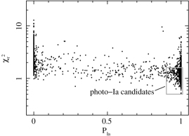
Figure 16.— $P_{\mathrm{Ia}}$ vs $\chi^{2}_{r}$ for the 2776 photometric candidates with no spectroscopic information. The 860 photometric SN Ia candidates are bounded by the gray box shown in the lower right.

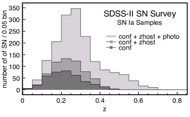
Figure 17.— Redshift distributions of the three SN Ia samples.

We now evaluate the light curves of the 445 candidates with spectroscopic redshift measurements of their host galaxies. Their SN types are unknown because there were no spectroscopic observations of these objects. Selection with $P_{z,{\mathrm{Ia}}}$ $\geq 0.90$, $\chi^{2}_{z,r}$ $\leq 1.8$, and $|$$z_{\mathrm{lc}}$ – $z_{\mathrm{spec}}$$|$/$\sigma_{z}<3$ results in 210 candidates shown in Figure 15. Based on the analysis presented in § 4.1, we expect this sample to have an efficiency of $\sim 89$%, purity of $\sim 94\%$, and a figure-of-merit of $\sim 0.84$. We refer to this sample of 210 candidates as the “$z_{\mathrm{host}}$-Ia sample”. Their candidate ID, coordinates, spectroscopic redshifts, and light curve fit results are listed in Table 3.

From the 2776 candidates with no spectroscopy, identifying sources with $P_{\mathrm{Ia}}$ $\geq 0.90$ and $\chi^{2}_{r}$ $\leq 1.6$ results in $860$ purely-photometric SN Ia candidates, which we refer to as the “photo-Ia sample”. The selection is shown in Figure 16. We expect this sample to have an efficiency of $\sim 92\%$, a purity of $\sim 94\%$, and a figure-of-merit of $0.86$. Its redshift distribution is shown in Figure 17. The mean redshift of the photo-Ia sample is $\bar{z}=0.31$ compared to $\bar{z}=0.22$ for the spectroscopically comfirmed sample. The full list of candidates is provided in Table 4. In addition to their coordinates, we provide the photometric light curve redshifts $z_{\mathrm{lc}}$ marginalized over all the other parameters. The reliability of these values is discussed in the following section.

The light curves of these candidates, as well as all of the other SN candidates, will be made available soon as part of the SDSS-II SN Survey Data Release.

6. Photometric Redshifts and Distances

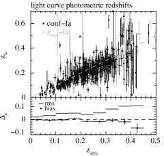
Figure 18.— Comparisons of $z_{\mathrm{spec}}$ and $z_{\mathrm{lc}}$ with a flat redshift prior for the spectroscopic SN Ia sample. The 387 SN Ia that pass the light curve quality cuts are shown in black while the 210 $z_{\mathrm{host}}$-Ia are indicated by gray crosses in the top panel. The bottom panel shows the mean $\Delta_{z}=(z_{\rm{lc}}-z_{\rm{spec}})/(1+z_{\rm{spec}})$ values in black circles and the RMS as horizontal bars in bins of 0.05 for the combined SN Ia + $z_{\mathrm{host}}$-Ia samples. The magnitude of the bias $|\Delta_{z}|$ is less than $0.02$ for $z<0.4$.

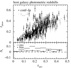
Figure 19.— Comparisons of $z_{\mathrm{spec}}$ and $z_{\mathrm{photo}}$, the photometric redshift of the SN Ia host galaxies from Oyaizu et al. (2008). There are fewer points here than in Figure 18 because there are many SN Ia with hosts that are below the detection limit of SDSS, and some galaxies are classfied as stars and therefore do not have $z_{\mathrm{photo}}$ values. The bottom panel shows the mean $\Delta_{z}$ values in black circles and the RMS as horizontal bars in bins of 0.05.

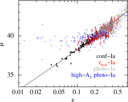
Figure 20.— Hubble diagram of the three SN Ia samples (conf-Ia in black, $z_{\mathrm{host}}$-Ia in red, and photo-Ia in light gray and blue in the online color version). The dark gray line represents $\Lambda$CDM. Spectroscopic redshift priors are used for the conf-Ia and $z_{\mathrm{host}}$-Ia samples. Flat redshifts priors are used for the photo-Ia sample. The redshift and distance of the photo-Ia are significantly correlated and their uncertainties are not shown for clarity. The outliers at low-$z$ are probably due to CC SN that are mis-classified as high-$A_{V}$ ($A_{V}>1$) SN Ia, which are shown in blue. Note that the majority of these points are significantly away from the $\Lambda$CDM Hubble relation.

The light curve redshifts $z_{\mathrm{lc}}$ are determined by marginalizing over the other four model parameters; $A_{V}$, $T_{\mathrm{max}}$, $\Delta m_{15}(B)$, and $\mu$. For each SN candidate, the posterior probability distribution function is constructed from the MCMC output. The redshifts listed in Table 4 correspond to the median $z_{\mathrm{lc}}$ and the $\pm 34.1$% ($1\sigma$) upper and lower limits.

We compare the spectroscopic redshifts $z_{\mathrm{spec}}$ with $z_{\mathrm{lc}}$ for the conf-Ia and $z_{\mathrm{host}}$-Ia samples and with the host galaxy photometric redshifts $z_{\mathrm{photo}}$ from Oyaizu et al. (2008) available in the SDSS DR8 database. As shown in Figure 18, $z_{\mathrm{lc}}$ and $z_{\mathrm{spec}}$ are in agreement with $|\Delta_{z}|<0.02$ ($\Delta_{z}\equiv(z_{\rm{lc}}-z_{\rm{spec}})/(1+z_{\rm{spec}})$) for $z_{\rm{spec}}<0.4$, but with a small redshift-dependent bias. The RMS scatter is $\Delta_{z,\rm{RMS}}=0.05$ below $z_{\rm{spec}}=0.30$ and increases to $0.1$ at $z=0.4$.

The sign and magnitude to this bias is similar to those found by Kessler et al. (2010a), who analyzed a subset of the higher S/N SDSS-II SN Ia light curves presented here using both MLCS and SALT-II. Interestingly, a similar bias is seen in their simulations. Rodney & Tonry (2010a) do not quote a value for the bias, but they state that a line with a slope of unity fits the $z_{\mathrm{spec}}$ vs. $z_{\mathrm{lc}}$ values for the first-year SDSS-II SN Ia sample with a $\chi^{2}_{r}$$=0.98$.

We also show in Figure 19 a comparison of $z_{\mathrm{spec}}$ with the host galaxy photometric redshift $z_{\mathrm{photo}}$ from Oyaizu et al. (2008). Here, there is a nearly constant bias of $\Delta_{z}\sim 0.03$ with an RMS scatter of $\Delta_{z,\rm{RMS}}\sim 0.05-0.10$.

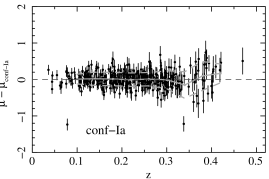
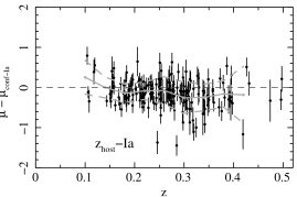
Figure 21.— (Top) The Hubble residuals of the conf-Ia sample relative to a simple quadratic Hubble relation. The solid line represents the mean residual and the dashed lines represent upper and lower rms values relative to the mean. The scatter ranges from $\sigma_{\mu}\sim 0.13$ mag to $\sigma_{\mu}\sim 0.30$ mag in the redshift interval $0.1<z<0.4$. (Bottom) Same except for the $z_{\mathrm{host}}$-Ia sample. The same quadratic has been subtracted from the measured distance modulus. The scatter here is larger and ranges from $\sigma_{\mu}\sim 0.2$ mag to $\sigma_{\mu}\sim 0.4$ mag in the same redshift range. There is also a small redshift-dependent offset.

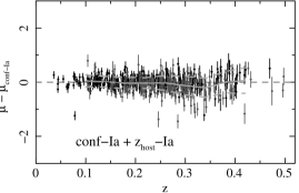
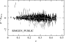
Figure 22.— (Top) Same as in Figure 21 for the combined conf-Ia + $z_{\mathrm{host}}$-Ia sample, which are labeled in black and light gray, respectively. The same quadratic function $\mu_{\rm{conf-Ia}}(z)$ has been subtracted from the measured distance modulus. The rms scatter is slightly larger than that of the conf-Ia sample only. (Bottom) Simulated SDSS-II SN from K10b. The black, light gray, and dark gray points represent SN Ia, SN II, and SN Ib/c, respectively, which pass all of the photometric SN Ia cuts ($P_{\mathrm{Ia}}$ $\geq 0.9$ and $\chi^{2}_{z,r}$ $<1.0$). The residuals shown are relative to a quadratic fit to the simulated SN Ia sample only, whereas the rms scatter shown is for the full sample. Note the slight redshift-dependent bias relative to the SN Ia mean.

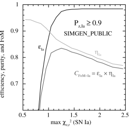
Figure 23.— Same as in Figure 10 for simulated SDSS-II SN from K10b except with an additional constraint of S/N $>7$ in two bands to approximately match the $z_{\mathrm{host}}$-Ia sample.

We show in Figure 20 the Hubble diagram of the 350 conf-Ia, 210 $z_{\mathrm{host}}$-Ia, and 860 photo-Ia samples. Distance modulus residuals of the conf-Ia and $z_{\mathrm{host}}$-Ia samples relative to a simple quadratic fit are shown in Figure 21. For the conf-Ia sample, the scatter around the mean Hubble relation is $\sigma_{\mu}=0.13$ mag at $z=0.1$ and increases monotonically to $\sigma_{\mu}=0.30$ mag at $z=0.4$. The same Hubble relation was subtracted from the $z_{\mathrm{host}}$-Ia sample, which is shown in the right panel of Figure 21. There is a noticeably larger scatter with $\sigma_{\mu}=0.2-0.4$ mag in the same redshift range. This is most likely due to contamination from non-Ia events, which we have estimated to be at the level of $\sim 6$% (approximately 1 out of 16 events in this sample is likely to be a CC SN). The slight deviation of the mean from zero is not statistically significant.

The Hubble diagram of the photo-Ia sample shows extreme outliers below $z\sim 0.1$. All of these points are significantly above the $\Lambda$CDM Hubble relation, and are most likely CC SN that are mis-classified as SN Ia. In fact, the majority of these events are classified by PSNID as extremely-underluminous, high-extinction ($A_{V}\gtrsim 1$) SN Ia. Since the underlying extinction distribution of SN Ia follows the relation $\propto e^{-A_{V}/\tau_{V}}$ with $\tau_{V}\sim 0.33$ (Kessler et al., 2009a), and given the smaller number of confirmed SN Ia in the same redshift interval, it is unlikely that all of these outlier events are underluminous, high-extinction SN Ia. Selecting only the candidates with $A_{V}<1$ eliminates most of these outliers at the cost of a somewhat reduced efficiency, but measurements of their host galaxy redshifts will also significantly help distinguish their types.

At higher redshifts, the mean Hubble relation of the photo-Ia sample is consistent with the conf-Ia and $z_{\mathrm{host}}$-Ia samples, but with a significantly larger scatter. Above $z\sim 0.2$, the rms scatter is $\sigma_{\mu}\sim 0.5-0.7$ mag, which is about a factor of $\sim 2$ larger than the scatter in the conf-Ia and $z_{\mathrm{host}}$-Ia samples in the same redshift range.

7. Comparisons with Simulations

The Hubble diagram for the combined conf-Ia + $z_{\mathrm{host}}$-Ia sample is shown in the top panel of Figure 22. The scatter is $\sigma_{\mu}=0.2$ mag at $z=0.1$ and increases to $\sigma_{\mu}=0.4$ mag at $z=0.4$, which is slightly larger than the scatter of the conf-Ia sample.

This degradation is probably due to contamination by CC SN events, but to test this hypothesis, we analyzed the sample of simulated SDSS-II SN from K10b. This simulation corresponds to 10 three-season search campaigns, and uses the actual seeing, photometric zeropoints, and weather from our observing seasons. The right panel in Figure 22 shows the Hubble diagram using all events that pass the same light curve quality cuts, as well as identical selection criteria in $P_{z,{\mathrm{Ia}}}$- $\chi^{2}_{z,r}$ space. Specifically, we select SN Ia candidates using $P_{z,{\mathrm{Ia}}}$ $\geq 0.9$ and $\chi^{2}_{z,r}$ $<1.0$, which is approximately where the efficiency and purity are equal at $\sim 0.90$ for this simulation. The efficiency, purity, and figure-of-merit curves are shown in Figure 23. The average S/N of the $z_{\mathrm{host}}$-Ia sample is higher than that of the simulations, so we require in the simulations S/N $>7$ in at least two of the $gri$ bands. The purity of 90% for this selection is slightly lower than the estimated purity of the $z_{\mathrm{host}}$-Ia sample.

The SN Ia Hubble digram was fitted to a quadratic function and the Hubble residuals of all candidates classified as SN Ia are shown in the bottom panel of Figure 22. Here, the CC SN events are shown in dark (SN Ib/c) and light gray (SN II) points. These false-positives are adding scatter and a small redshift-dependent systematic shift relative to the SN Ia distances, which are represented by black points. The Hubble scatter around the mean for this simulation is $\sigma_{\mu}=0.2-0.4$ mag, which is similar to the that of the $z_{\mathrm{host}}$-Ia sample over the entire redshift range. The larger scatter seen in the conf-Ia + $z_{\mathrm{host}}$-Ia sample is, therefore, most likely due to mis-classified CC SN as reproduced in these simulations.

This set of simulated SDSS-II SN also includes a spectroscopic SN Ia sample selected based on our spectroscopic follow-up strategies, and represents our conf-Ia. The Hubble residual scatter of this spectroscopic sample ranges from $\sigma_{\mu}\sim 0.13$ mag to $\sigma_{\mu}\sim 0.30$ mag in the redshift interval $0.1<z<0.4$, which is nearly identical to the observed scatter of the conf-Ia sample.

8. Summary and Conclusions

We have identified $1070$ photometric SN Ia candidates from the SDSS-II SN Survey data. This sample is more than three times larger than the spectroscopically confirmed SN Ia sample with good light curves, and is estimated to include $\sim 91$% of all SN Ia candidates detected by the survey with a purity of $\sim 94$% ($\sim 6$% contamination). This estimate of the purity, however, is based on a limited number of spectroscopically confimred CC SN, most of which are nearby, bright events and are therefore not representative of the majority of the contaminating events. As shown in Figure 6, the majority of our photometric candidates have peak $r$-band S/N$<10$, where we have only a handful of spectroscopic SN candidates. To obtain a better characterization of the contaminating sources, confirmation is needed for a much larger sample of faint CC SN that are comparable in apparent brightness to the photo-Ia sample. As also advocated by Richards et al. (2011), future surveys that rely on photometric identification should obtain spectra of SN candidates over the full range of the S/N of the photometric candidates of interest.

The Hubble digram with photometric classification and host galaxy spectroscopic redshift priors show a slight increase in scatter over the confirmed SN Ia sample, which is consistent with them being due to mis-classified CC SN. There is no significant redshift-dependent offset in the derived distances compared to the conf-Ia sample. Simulations confirm these findings.

Photometric redshifts estimated from the multi-band light curves are unbiased below $z\sim 0.2$ with an rms dispersion of $\sigma_{z}\sim 0.05$. There is a redshift-dependent bias above $z\sim 0.2$ where the mean redshift difference $\langle z_{\mathrm{lc}}-z_{\mathrm{photo}}\rangle$ is between $-0.04$ and $-0.02$. The rms dispersion is $\sigma_{z}\sim 0.05-0.10$. The Hubble diagram of the photo-Ia sample also exhibits outliers and redshift-dependent biases. Although the distance and redshift accuracies at present are not yet sufficient for cosmology, the large sample can still be used for studies of the SN Ia rate as a function of redshift, correlations between SN light curves and host galaxy properties, and other studies that do not involve joint constaints on both redshift and distance.

We conclude that cosmology with future large-scale SN surveys should at the minimum measure host galaxy spectroscopic redshifts for the Hubble digram. A subset of the SN candidates must be observed spectroscopically to study the photometric classification efficiency and purity. Spectroscopy should target candidates with S/N down to the magnitude limit where photometric classification is expected to work. Cosmology with photometry alone, however, requires further investigation with realistic simulations in order to understand and characterize their systematic biases and uncertainties, and how they depend on the SN Ia candidate selection criteria.

References

- Abazajian et al. (2009) Abazajian, K. N., et al. 2009, ApJS, 182, 543
- Aldering et al. (2006) Aldering, G., et al. 2006, ApJ, 650, 510
- Astier et al. (2006) Astier, P., et al. 2006, A&A, 447, 31
- Bailey et al. (2009) Bailey, S., et al. 2009, A&A, 500, L17
- Barris & Tonry (2004) Barris, B. J., & Tonry, J. L. 2004, ApJ, 613, L21
- Cardelli, Clayton, & Mathis (1989) Cardelli, J. A., Clayton, G. C., & Mathis, J. S., ApJ, 345, 245
- Conley et al. (2011) Conley, A., et al. 2011, ApJS, 192, 1
- Contreras et al. (2009) Contreras, C., et al. 2010, AJ, 139, 519
- D’Andrea et al. (2010) D’Andrea, C. B., et al. 2010, ApJ, 708, 661
- Dahlen et al. (2004) Dahlen, T., et al. 2004, ApJ, 613, 189
- Dahlen et al. (2008) Dahlen, T., Strolger, L.-G., & Riess, A. G. 2008, ApJ, 681, 462
- Dawson et al. (2009) Dawson, K. S., et al. 2009, AJ, 138, 1271
- Dilday et al. (2008) Dilday, B., et al. 2008, ApJ, 682, 262
- Dilday et al. (2010) Dilday, B., et al. 2010, ApJ, 713, 1026
- Eisenstein et al. (2001) Eisenstein, D. J., et al. 2001, AJ, 122, 2267
- Filippenko et al. (2001) Filippenko, A. V., Li, W. D., Treffers, R. R., & Modjaz, M. 2001, IAU Colloq. 183: Small Telescope Astronomy on Global Scales, 246, 121
- Flaugher et al. (2010) Flaugher, B. L., et al. 2010, Proc. SPIE, 7735,
- Folatelli et al. (2010) Folatelli, G., et al. 2010, AJ, 139, 120
- Freedman et al. (2009) Freedman, W. L., et al. 2009, ApJ, 704, 1036
- Frieman et al. (2008) Frieman, J. et al. 2008, AJ, 135, 338
- Fukugita et al. (1996) Fukugita, M., Ichikawa, T., Gunn, J. E., Doi, M., Shimasaku, K., & Schneider, D. P. 1996, AJ, 111, 1748
- Ganeshalingam et al. (2010) Ganeshalingam, M., et al. 2010, ApJS, 190, 418
- Gong et al. (2009) Gong, Y., Cooray, A., & Chen, X. 2009, arXiv:0909.2692
- Graur et al. (2011) Graur, O., et al. 2011, arXiv:1102.0005
- Gunn et al. (1998) Gunn, J. E., et al. 1998, AJ, 116, 3040
- Gunn et al. (2006) Gunn, J. E., et al. 2006, AJ, 131, 2332
- Guy et al. (2010) Guy, J., et al. 2010, A&A, 523, A7
- Hamuy et al. (1996a) Hamuy, M., Phillips, M. M., Suntzeff, N. B., Schommer, R. A., Maza, J., & Aviles, R. 1996, AJ, 112, 2391
- Hicken et al. (2009) Hicken, M., Wood-Vasey, W. M., Blondin, S., Challis, P., Jha, S., Kelly, P. L., Rest, A., & Kirshner, R. P. 2009, ApJ, 700, 1097
- Holtzman et al. (2008) Holtzman, J. et al., 2008, AJ, 136, 2306
- Jha et al. (2006a) Jha, S., et al. 2006, AJ, 131, 527
- Jha et al. (2006b) Jha, S., Branch, D., Chornock, R., Foley, R. J., Li, W., Swift, B. J., Casebeer, D., & Filippenko, A. V. 2006, AJ, 132, 189
- Johnson & Crotts (2006) Johnson, B. D., & Crotts, A. P. S. 2006, AJ, 132, 756
- Kessler et al. (2009a) Kessler, R., et al. 2009, ApJS, 185, 32
- Kessler et al. (2009b) Kessler, R., et al. 2009, PASP, 121, 1028
- Kessler et al. (2010a) Kessler, R., et al. 2010, ApJ, 717, 40
- Kessler et al. (2010b) Kessler, R., et al. 2010, PASP, 122, 1415
- Kim & Miquel (2007) Kim, A. G., & Miquel, R. 2007, Astroparticle Physics, 28, 448
- Kunz et al. (2007) Kunz, M., Bassett, B. A., & Hlozek, R. A. 2007, Phys. Rev. D, 75, 103508
- Kuznetsova & Connolly (2007) Kuznetsova, N. V., & Connolly, B. M. 2007, ApJ, 659, 530
- Lampeitl et al. (2009) Lampeitl, H., et al. 2010, MNRAS, 401, 2331
- Law et al. (2009) Law, N. M., et al. 2009, PASP, 121, 1395
- Li et al. (2003) Li, W., et al. 2003, PASP, 115, 453
- LSST Science Collaborations et al. (2009) LSST Science Collaborations 2009, arXiv:0912.0201
- Matheson et al. (2008) Matheson, T., et al. 2008, AJ, 135, 1598
- McClelland et al. (2010) McClelland, C. M., et al. 2010, in preparation
- Miknaitis et al. (2007) Miknaitis, G., et al. 2007, ApJ, 666, 674
- Nugent, Kim, & Perlmutter (2002) Nugent, P., Kim, A., & Perlmutter, S. 2002, PASP, 114, 803
- Oyaizu et al. (2008) Oyaizu, H., Lima, M., Cunha, C. E., Lin, H., Frieman, J., & Sheldon, E. S. 2008, ApJ, 674, 768
- Palanque-Delabrouille et al. (2010) Palanque-Delabrouille, N., et al. 2010, A&A, 514, A63
- Panagia (2003) Panagia, N. 2003, Supernovae and Gamma-Ray Bursters, ed. K. Weiler, Lecture Notes in Phyiscs, Vol. 598 (Springer: Berlin), 113
- Perlmutter et al. (1999) Perlmutter, S., et al. 1999, ApJ, 517, 565
- Phillips (1993) Phillips, M. M. 1993, ApJ, 413, L105
- Phillips et al. (1999) Phillips, M. M., Lira, P., Suntzeff, N. B., Schommer, R. A., Hamuy, M., & Maza, J. 1999, AJ, 118, 1766
- Phillips et al. (2007) Phillips, M. M., et al. 2007, PASP, 119, 360
- Poznanski et al. (2002) Poznanski, D., Gal-Yam, A., Maoz, D., Filippenko, A. V., Leonard, D. C., & Matheson, T. 2002, PASP, 114, 833
- Poznanski et al. (2007a) Poznanski, D., Maoz, D., & Gal-Yam, A. 2007, AJ, 134, 1285
- Poznanski et al. (2007b) Poznanski, D., et al. 2007, MNRAS, 382, 1169
- Prieto et al. (2007) Prieto, J. L., et al. 2007, arXiv:0706.4088
- Pskovskii (1977) Pskovskii, I. P. 1977, Soviet Astronomy Letters, 3, 215
- Rau et al. (2009) Rau, A., et al. 2009, PASP, 121, 1334
- Richards et al. (2002) Richards, G. T., et al. 2002, AJ, 123, 2945
- Richards et al. (2011) Richards, J. W., Homrighausen, D., Freeman, P. E., Schafer, C. M., & Poznanski, D. 2011, arXiv:1103.6034
- Richardson et al. (2002) Richardson, D., Branch, D., Casebeer, D., Millard, J., Thomas, R. C., & Baron, E. 2002, AJ, 123, 745
- Riess et al. (1998) Riess, A. G., et al. 1998, AJ, 116, 1009
- Riess et al. (1999) Riess, A. G., et al. 1999, AJ, 117, 707
- Riess et al. (2004a) Riess, A. G., et al. 2004, ApJ, 607, 665
- Riess et al. (2004b) Riess, A. G., et al. 2004, ApJ, 600, L163
- Riess et al. (2007) Riess, A. G., et al. 2007, ApJ, 659, 98
- Rodney & Tonry (2009) Rodney, S. A., & Tonry, J. L. 2009, ApJ, 707, 1064
- Rodney & Tonry (2010a) Rodney, S. A., & Tonry, J. L. 2010, ApJ, 715, 323
- Rodney & Tonry (2010b) Rodney, S. A., & Tonry, J. L. 2010, ApJ, 723, 47
- Sako et al. (2008) Sako, M., et al., 2008, AJ, 135, 348
- Schneider et al. (2010) Schneider, D. P., et al. 2010, AJ, 139, 2360
- Scolnic et al. (2009) Scolnic, D. M., Riess, A. G., Huber, M. E., Rest, A., Stubbs, C. W., & Tonry, J. L. 2009, ApJ, 706, 94
- Sollerman et al. (2009) Sollerman, J., et al. 2009, ApJ, 703, 1374
- Strauss et al. (2002) Strauss, M. A., et al. 2002, AJ, 124, 1810
- Sullivan et al. (2006) Sullivan, M., et al. 2006, AJ, 131, 960
- Wang et al. (2007) Wang, Y., Narayan, G., & Wood-Vasey, M. 2007, MNRAS, 382, 377
- Wang (2007) Wang, Y. 2007, ApJ, 654, L123
- Wood-Vasey et al. (2007) Wood-Vasey, W. M., et al. 2007, ApJ, 666, 694
- York et al. (2000) York, D. G., et al. 2000, AJ, 120, 1579
- Zheng et al. (2008) Zheng, C. et al., 2008, AJ, 135, 1766