The nature and cause of spectral variability in LMC X–1

Abstract

We present the results of a long-term observation campaign of the extragalactic wind-accreting black-hole X-ray binary LMC X–1, using the Proportional Counter Array on the Rossi X-Ray Timing Explorer (RXTE). The observations show that LMC X–1’s accretion disk exhibits an anomalous temperature-luminosity relation. We use deep archival RXTE observations to show that large movements across the temperature-luminosity space occupied by the system can take place on time scales as short as half an hour. These changes cannot be adequately explained by perturbations that propagate from the outer disk on a viscous timescale. We propose instead that the apparent disk variations reflect rapid fluctuations within the Compton up-scattering coronal material, which occults the inner parts of the disk. The expected relationship between the observed disk luminosity and apparent disk temperature derived from the variable occultation model is quantitatively shown to be in good agreement with the observations. Two other observations support this picture: an inverse correlation between the flux in the power-law spectral component and the fitted inner disk temperature, and a near-constant total photon flux, suggesting that the inner disk is not ejected when a lower temperature is observed.

1 Introduction

LMC X–1 is (with Cyg X–1 (catalog )) one of only two known persistently luminous x-ray binaries consisting of a black hole accreting the wind of a massive blue star. The $10.91\pm 1.41M_{\odot}$ black hole is in a $3.90917\pm 0.00005$ day orbit (Orosz et al., 2009) about an O7 III companion (Cowley et al., 1995). As the companion both drives a strong wind and is far from filling its Roche lobe, wind accretion feeds the black hole (Nowak et al., 2001). The system, which accretes at an average of $0.16L_{Edd}$ (Gou et al., 2009) has never been observed in the low/hard state (Wilms et al., 2001). Gou et al. (2009) used x-ray data, including some of the RXTE observations we use here, to derive a spin parameter $\alpha=0.92(+0.05,-0.07)$ for the black hole in LMC X–1 using fits to the disk blackbody component of the spectrum.

LMC X–1 (catalog )’s persistent occupation of the high/soft state contrasts with the behavior of Cyg X–1 (catalog ), which it closely resembles in other respects. Cyg X–1 harbors a $\sim 10M_{\odot}$ black hole (Herrero et al., 1995) in a $5.6$ day orbit (Paczynski, 1974) about an O9.7 Iab companion (Bolton, 1972). Though Cyg X–1 (catalog ) is also a wind-accreting system, its typical luminosity in the high state is $\sim 0.03L_{Edd}$ (Gierliński et al., 1999), which is much lower than LMC X–1 (catalog )’s. This implies that the black hole in LMC X–1 accretes at a higher rate than its counterpart in Cyg X–1 (catalog ), perhaps because the companions’ wind speeds and densities differ, or that accretion mechanisms with different radiative efficiencies are taking place. In addition, Cyg X–1 (catalog ) exhibits well-documented transitions between the high/soft state and the low/hard state (Agrawal et al., 1972; Baity et al., 1973; Heise et al., 1975; Holt et al., 1976, 1975; Sanford et al., 1975). LMC X–1, in contrast, displays persistent soft-state emission (Nowak et al., 2001; Wilms et al., 2001). While both LMC X–1 (catalog ) and Cyg X–1 (catalog )’s softest states can be fitted with a power law plus disk blackbody model, they also differ markedly. The traditional soft state model, in which the disk blackbody dominates the energy spectrum, accurately fits LMC X–1 (catalog )’s spectra (Ebisawa et al., 1989; Yao et al., 2005). Cyg X–1 (catalog )’s spectra, however, are energetically dominated by the power law in both the hard and soft states. Thus, while these two systems have similar companions and orbital properties, they differ in their spectral characteristics and evolution.

An even more interesting comparison can be made between LMC X–1 (catalog ) and LMC X–3 (catalog ), a black-hole binary that accretes via Roche-lobe overflow at comparable luminosity, as a means of highlighting the observational differences between disk and wind accretion. Much of this paper will be devoted to pointing out and interpreting these differences.

LMC X–3 (catalog )  is a persistently bright x-ray binary in the Large Magellanic Cloud, and is the only other system with a dynamically confirmed black hole. As such, it provides a useful counterpoint to the wind-accreting black hole binary systems mentioned above. LMC X–3 is a $9M_{\odot}$ black hole (van der Klis et al., 1985) with an evolved B5 companion (Soria et al., 2001). A detailed listing of the system’s dynamical properties, along with those of LMC X–1 (catalog ) and Cyg X–1 (catalog ), is provided in Table 1. Differences between the systems are expected to reflect differences in the accretion flows resulting from wind versus Roche-lobe overflow accretion: LMC X–3 accretes high angular momentum material through its first Lagrange point, while LMC X–1 accretes low angular momentum material from its companion’s stellar wind. LMC X–3 and LMC X–1 share spectral signatures of a persistent accretion disk, though LMC X–1’s disk spectrum defies the $L\propto T^{4}$ relation (Mitsuda et al., 1984; Dunn et al., 2010).

Table 1: System parameters for LMC X–1, LMC X–3, and Cygnus X–1, with references in parenthesis. The Eddington luminosity for each source was calculated from black hole mass.

	LMC X–1 (catalog )	LMC X–3 (catalog )	Cyg X–1 (catalog )
Distance (kpc)	$48.10\pm 2.22$ (1)	$52.0\pm 0.6$ (2)	$2.5$ (3)
Black Hole Mass ($M_{\odot}$)	$10.91\pm 1.41$ (1)	$11.1\pm 1.4$ (4)	$10.1$ (5)
System Inclination (degrees)	$36.38\pm 1.92^{\circ}$ (1)	$50.0^{\circ}\leq i\leq 70.0^{\circ}$ (12)	$36^{\circ}<i<67^{\circ}$ (11)
Companion Type	O7 III (8)	B5 IV (6)	O9.7 Iab (5)
Companion Mass ($M_{\odot}$)	$31.79\pm 3.48$ (1)	$4.0\leq M\leq 4.7$ (6)	$17.8$ (5)
Companion Radius ($R_{\odot}$)	$17.0\pm 0.8$ (1)	$4.4$ (6)	$22.7\pm 2.3$ (7)
Orbital Period (days)	$3.90917\pm 0.00005$ (1)	$1.70479\pm 0.00004$ (5)	$5.6$ (3)
Average Soft State Luminosity (% LEdd)	$\sim 16\%$ (8)	$\leq 30\%$ (9)	$\sim 3\%$ (10)

(1) Orosz et al. (2009); (2) di Benedetto (1997); (3) Paczynski (1974); (4) Gierliński et al. (2001); (5) Herrero et al. (1995); (6) Soria et al. (2001); (7) Ziółkowski (2005); (8) Gou et al. (2009); (9) Nowak et al. (2001); (10) Gierliński et al. (1999); (11) Davis & Hartmann (1983); (12) van der Klis et al. (1985).

This paper examines how LMC X–1 (catalog )’s spectral properties and evolution fit with, and possibly extend, existing black hole binary accretion models. In particular, our results ultimately indicate that LMC X–1 (catalog )’s spectral behavior is consistent with sporadic obscuration of the innermost part of a stable accretion disk.

Section 2 of this paper presents the data processing and spectral fitting techniques employed in obtaining the results presented in Section 3. Section 4 discusses how LMC X–1 (catalog )’s unique spectral properties can be reconciled with existing accretion flow models, while Section 5 presents our conclusions and possible avenues for further investigation.

2 Observations and Data Analysis

The data analyzed in this work fall into two categories. The bulk of the observations come from our twice-weekly RXTE monitoring campaign of LMC X–1 (catalog ) and LMC X–3 (catalog ). The LMC X–1 (catalog ) data were complemented by long, individual RXTE observations available on the HEASARC. These data were reduced and analyzed using identical processes. The two classes of LMC X–1 (catalog ) observations prove useful for probing different timescales of spectral variations.

2.1 Observations

The main observing campaign consisted of brief, uninterrupted observations of LMC X–1 (catalog ) and LMC X–3 (catalog ), conducted twice a week since August 2007 and March 2006, respectively. These observations ranged in length between 506 and 5470 seconds, with average lengths of 1661 seconds for LMC X–1 (catalog ) and 1877 seconds for LMC X–3 (catalog ). The LMC X–1 (catalog ) observations were offset from the source by 15.764’ to reduce contamination from the nearby pulsar PSR B0540-69. These twice-weekly observations give reliable pictures of the typical X-ray spectra of LMC X–1 (catalog ) and LMC X–3 (catalog ) over significant periods of time. While this is a major strength of these data sets, it also a weakness, in that they only have the capacity to reveal spectral variations that emerge over a minimum of several days.

To examine shorter timescale variations in LMC X–1 (catalog ), we take advantage of the seventeen deep archival RXTE observations listed in Table 2. We “chopped” these data sets into shorter spectra (less than 90 min) corresponding to one orbit of the RXTE spacecraft. These chopped archival observations can reveal spectral changes that emerge over fractions of a day.

Observation ID	UT (yyyy-mm-dd)	Start Date (MJD)	Total Exposure (s)	Sub-Observations
20188-01-02-00	1996-12-30	50447.438	9919	4
20188-01-03-00	1997-01-18	50466.347	9941	3
20188-01-05-00	1997-03-09	50516.354	10189	4
20188-01-06-00	1997-03-21	50528.004	10625	4
20188-01-07-00	1997-04-16	50554.193	11484	3
20188-01-14-00	1997-09-09	50700.695	10174	4
20188-01-18-00	1997-10-10	50731.611	11436	3
30087-01-02-00	1998-01-25	50838.667	10017	3
30087-01-03-00	1998-02-20	50864.370	9948	4
30087-01-04-00	1998-03-12	50884.495	10007	7
30087-01-06-00	1998-05-06	50939.149	11396	4
30087-01-07-00	1998-05-28	50961.101	5966	2
30087-01-08-00	1998-06-28	50992.097	9921	4
30087-01-09-00	1998-07-19	51013.909	10094	4
80118-01-06-02	2004-01-11	53015.340	10908	3
80118-01-07-00	2004-01-12	53016.258	10788	3
80118-01-08-00	2004-01-10	53014.236	6608	2

Table 2: Summary of the deep archival RXTE observations used to constrain the power law index, and to find upper limits on the apparent timescale of disk luminosity evolution. The former used only the parts of the spectra above 12 keV, while the latter relied only on regions of the spectra below 12 keV.

2.2 Data Analysis

All data were reduced using standard HEASOFT v6.7 tools. Data taken within 30 minutes after the satellite exited the South Atlantic Anomaly (SAA), or when the source was at less than 10^∘ elevation above Earth’s limb, were excluded from subsequent analysis. All observations only considered data from the second proportional counter unit (PCU2) of RXTE’s Proportional Counter Array (PCA), due to its consistent performance throughout the mission. The mission-long faint background model pca_bkgd_cmfaintl7_eMv20051128.mdl was used in this analysis, as the total count rate for both LMC sources lies below 40 photons/s/PCU. Data were extracted using the Standard2 data mode.

We used uniform XSPEC v12.5.1 (Arnaud, 1996) fitting procedures for all data. Per RXTE recommendation (Jahoda et al., 2006), systematic errors of 1% were added in quadrature to the Poisson counting noise errors. Because the detector response is poorly understood within the first three PCA channels, we exclude those channels from our analysis, resulting in a lower energy threshold just under 3 keV. Above 16 keV, the signal to noise ratio for both sources is too low to provide useful fits to the data, so our fits also exclude all data for energies over 16 keV. A 29% decrease in the PCA efficiency (Jahoda et al., 2006) relative to an on-axis source resulted from the 15.764’ off-axis pointing of our LMC X–1 (catalog ) observations. All fluxes derived from the off-axis LMC X–1 (catalog )observations were multiplied by a factor of 1.4 to account for this efficiency factor. Representative spectra, model fits, and fit residuals for LMC X–1 (catalog ) and LMC X–3 (catalog ) are presented in Figures 1 and 2, respectively.

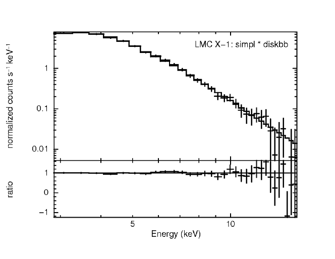
normal

Figure 1: Fit and data-to-model ratio for LMC X–1 (catalog ) data fit by the multi-colored disk and simpl (power-law) spectral model.

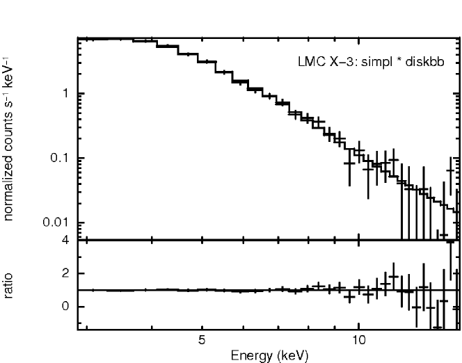
Figure 2: Fit and data-to-model ratio for LMC X–3 (catalog ) data fitted by multi-colored disk and simpl (power-law) spectral model.

Spectra were fitted with a disk blackbody plus power law emission model. The first spectral component is a multicolored blackbody spectrum generated by the accretion disk, which is accounted for using the standard diskbb XSPEC model (Mitsuda et al., 1984). The simpl XSPEC model (Steiner et al., 2009) accounts for the power-law emission, which extends to high energies, and which is thought to be caused by Compton up-scattering of disk photons through a population of hotter electrons (Shapiro et al., 1976). A pure power-law model runs the risk of promoting spectral fits that inaccurately trade disk luminosity for coronal energy flux. The XSPEC simpl model avoids this by turning over at low energies, and by convolving an arbitrary input photon spectrum with the specified Compton scattering prescription. It is, therefore, less prone to overestimating the amount of non-thermal emission. Simpl can account for either pure photon up-scattering, or for both up- and down-scattering. Because the average energy of coronal electrons is two orders of magnitude higher than the highest disk blackbody temperature, coronal emission from our sources can be safely approximated by pure up-scattering.

Finally, to account for photoelectric absorption within the intervening ISM, we convolve the compound model with phabs. Our approach does not conflict with the findings of Levine & Corbet (2006) and Hanke et al. (2010), which detect orbital phase variations in the absorption column towards LMC X-1. These orbital phase variations suggest that LMC X-1’s companion drives a significant wind. While the variable column density significantly effects LMC X-1’s observed soft x-ray emission, it does not impact the higher energy range examined in this analysis.

Table 3 lists the fitting parameters and results from the following fitting procedure. The simpl power law index, the absorption column, and the inverse Compton scattering flag are all frozen at the listed values. The absorption column densities are drawn from Nowak et al. (2001) for both LMC X–1 (catalog ) and LMC X–3 (catalog ). The innermost disk temperature starts, but is not frozen, at the physically reasonable energy of 1 keV. The spectral fits output the inverse Compton photon scattering fraction, the innermost disk temperature, the overall normalization of the diskbb model component, and $\chi^{2}$ goodness-of-fit statistics. Once the model has been fitted to the data, it is used to calculate both comprehensive and component-specific photon and energy fluxes.

		LMC X–1 (catalog )	LMC X–3 (catalog )
Inputs (frozen)	nH ($cm^{-2}$)	$7.2\times 10^{21}$ (1)	$3.2\times 10^{20}$ (1)
	$\Gamma$	$2.68$	$2.34$ (2)
	Scattering Flag	1	1
Outputs (average values)	$kT_{e}$ (keV)	$0.90\pm 0.06$	$1.07\pm 0.18$
	$f_{sc}$	$0.13\pm 0.07$	$0.08\pm 0.17$
	$\chi^{2}/$d.o.f.	$0.79\pm 0.24$	$0.79\pm 0.77$

Table 3: Input parameters and results for the phabs $\times$ (simpl $\times$ diskbb) fits to LMC X–1 (catalog ) and LMC X–3 (catalog ) data, with citations in parenthesis. Uncertainties in the outputs correspond to single standard deviations of the values about their average. Fixing simpl’s scattering flag at a value of 1 forces the fits to account for only up-scattering. (1) Nowak et al. (2001); (2) Smith et al. (2007)

The low photon counts from both LMC X–1 and LMC X–3 limit the usable energy range in our 1.5 ksec observations to no higher than 16 keV. With counting statistics of this quality, it is not possible to simultaneously constrain both the power-law index and the inner-disk temperature. Since our observations cannot determine all six of the parameters in the $\texttt{phabs}\times\texttt{simpl}\times\texttt{diskbb}$ model (see table), we freeze the power-law index, which is the most stable at long time scales. The deep archival observations of LMC X–1, prior to being chopped into orbit-by-orbit sections, have sufficient photons to simultaneously constrain all disk and power-law fit parameters. We use the average power law index derived from these long observations, which is consistent with a single value, to fix the power law index for all of the single-orbit LMC X–1 spectra. For LMC X–3, we employ the average power law index found in the same way by Smith et al. (2007). In both cases, the values for all deep pointings are statistically consistent with the average.

3 Results

We find that LMC X–1 (catalog ) remained in the soft state over the entire observation program, and has an anomalous disk-temperature-versus-luminosity relation relative to the expectation of a disk blackbody.

Figure 3 demonstrates how the luminosity of a typical accretion disk, such as the one present in LMC X–3 (catalog )’s soft state, follows the expected modified $L\propto T_{in}^{4}$ Stefan-Boltzmann relation (Mitsuda et al., 1984). The line in Figure 3, which represents this relation, was not fitted to the data beyond finding a suitable normalization constant. The relation nevertheless fits the data very well, aside from the highly uncertain points at low luminosities and high temperatures. These points come from observations taken after Feb. 23, 2009 (MJD 54885), when LMC X–3 transitioned from a disk-dominated high/soft state to the low/hard state. The fitting routine we employ is not appropriate for the low/hard state, during which disk emission is suppressed and the power-law index hardens significantly. The poorly constrained values that appear in the lower right corner of Figure 4, well away from the Stefan-Boltzmann relation, result from using a high/soft state model to fit low/hard state data.

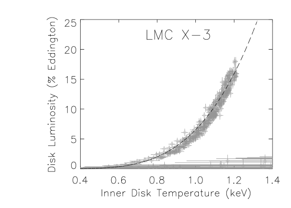
Figure 3: The disk temperature-luminosity relationship observed in LMC X–3 (catalog ). The dashed line is the modified accretion disk Stefan-Boltzmann relationship. The points at low luminosities and high temperatures, which lie far from the model, are due to a transition to the low/hard state towards the end of the observing campaign.

Figure 4 similarly shows the disk temperature-luminosity relation for LMC X–1. The dashed lines are two normalizations of the same Stefan-Boltzmann relation used in Figure 4, and clearly cannot fit the data.

Figure 4: The disk temperature-luminosity relationship observed in LMC X–1 (catalog ). The dashed lines are the modified accretion disk Stefan-Boltzmann relationship shown in Figure 3, and differ only in their overall normalization constants.

Figure 5 compares how the inner disk temperatures of LMC X–3 (catalog ) and LMC X–1 (catalog ) vary over time. The figure shows only a subset of the total observing campaign in order to better display short term variations from each source. The change in disk temperature from one observation to the next is markedly more continuous for LMC X–3 (catalog ) than for LMC X-1. Over longer time periods, however, LMC X–3 (catalog )’s inner disk temperature evolves significantly. Such long-term disk temperature evolution is absent in LMC X–1 (catalog ).

Figure 5: The innermost disk temperature plotted as a function of observation date for LMC X–3 (catalog ) (top) and LMC X–1 (catalog )(bottom).

Figure 6 shows how LMC X–1 (catalog )’s inner disk temperature and luminosity varied over the course of two of the archival observations listed in Table 2. The bottom panel shows data from the longest observation, while the top panel shows data from an observation with a typical number of exposure intervals.

The inner disk appears to evolve over a period of several hours. Rather than evolving along the Stefan-Boltzmann relation, the disk temperature and luminosity fall along a line of a very different slope. The order of the points is not uniform along this line either, suggesting motion faster than has been resolved by the data.

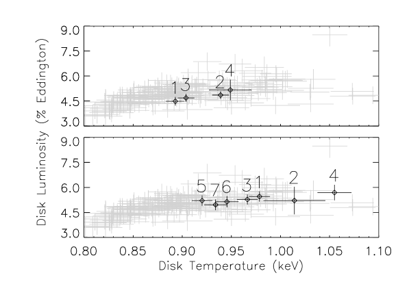
Figure 6: LMC X–1 (catalog ) inner disk temperature vs. luminosity over the course of two representative archival observations. The top panel shows observation 20188-01-05-00, while the lower panel shows observation 30087-01-04-00. Black points, representing subsections of the archival observation, are numbered in chronological order. Gray points represent the data from our own observing campaign, and provide a basis for comparison.

Figure 7 shows LMC X–1 (catalog )’s variability in disk, coronal, and total luminosities, as well as in the total photon emission rate, over the course of our observing program. The mild discrepancy between LMC X-1’s overall accretion luminosity as presented here and in Gou et al. (2009) comes from the narrower energy range we employ in calculating the source’s overall flux. Both analyses, however, find similar disk-to-coronal flux ratios in LMC X-1. Percent variation, defined as $\textrm{standard deviation}/\textrm{mean}$, quantifies the extent to which the values in each panel vary. The system’s disk luminosity shows $14.5$ % variation, while its coronal up-scattering luminosity shows $51.8$ % variation. The system’s overall x-ray luminosity has $15.2$ % variation. The total photon flux from LMC X-1 is the system’s most stable feature, with only $12.5$ % variation. While the total number of photons emanating from the system remains relatively steady, the amount of energy that the corona contributes to the total emission varies significantly.

Figure 7: From top to bottom: disk luminosity, coronal luminosity, total photon emission rate, and total luminosity of LMC X–1 (catalog )vs. observation date. Luminosities are shown in terms of the source’s Eddington luminosity.

Figure 8 displays the relation between LMC X–1 (catalog )’s inner disk temperature and the inverse Compton scattering fraction. While observations with cooler disk temperatures and higher scattering fractions suffer larger fitting uncertainties, a Pearson correlation analysis confirms the existance of a statistically significant negative correlation between these two parameters, even when the two upper-leftmost points in Figure 8 are removed. Since the scattering fraction maps directly to the inverse Compton optical depth, Figure 8 shows that the inner edge of the disk appears cooler when there is more coronal material.

Figure 8: The fraction of total disk seed photons that undergo Compton up-scattering versus the inner disk temperature.

4 Discussion and Conclusions

LMC X–1’s apparent defiance of the Stefan-Boltzmann relation may stem from variations in the disk itself, or from variations in the scattering medium surrounding it. Because the total number of photons is more nearly constant than the disk luminosity (see Figure 7), variations in the number of photons diverted to the power law by the corona seem more likely to explain the anomalous temperature/luminosity relations than variations within the disk itself.

The first step in quantitatively distinguishing between these two explanations for the anomalous disk relation is to compare the observed disk variation timescales to timescales inherent to the disk and to the corona. In Figure 6, LMC X–1 (catalog ) ’s disk randomly samples a wide swath of the temperature parameter space in the space of a few hours. Individual points in the archival observation are separated by an average of 2320 s, which provides an estimate of the timescale for apparent disk variations. We can compare this value to the disk’s viscous timescale to assess whether the disk’s structure is capable of changing over such a brief interval of time.

The disk’s viscous timescale scales with both radius and viscosity, as (Frank et al., 2002)

$$t_{visc}\sim\frac{R^{2}}{\nu}$$ (1)

The circularization radius, $R_{circ}$, of the accreted wind material gives a lower limit for the outer disk radius. The disk radius, and therefore the viscous timescale, may actually be larger due to outward angular momentum transfer. Since we are primarily concerned with finding a lower limit on the viscous timescale, however, $R_{circ}$ provides a conservative value of the disk radius. The circularization radius is defined as the radius at which the accreted matter’s angular momentum due to Keplerian motion equals the angular momentum it carried upon initial capture by the black hole. Following Frank et al. (2002) we assume that the wind’s initial angular momentum about the black hole goes as

$$l\sim\frac{1}{4}\omega R_{acc}^{2}$$ (2)

where $R_{acc}$ represents the black hole’s gravitational capture radius, and $\omega$ is the black hole’s orbital angular velocity about the companion. From there, we obtain

$$R_{circ}=\frac{G^{3}M_{BH}^{3}\omega^{2}}{v_{rel}^{8}}\textrm{.}$$ (3)

where $M_{BH}$ represents mass of the black hole, and

$$v_{rel}^{2}=v_{w}^{2}+v_{orb}^{2}\textrm{.}$$ (4)

Therefore, the disk’s size is strongly dependent on the speed of the stellar wind, which undergoes line-driven acceleration (Castor et al., 1975; Owocki, 1994; Kudritzki & Puls, 2000). The wind’s velocity increases with distance from the star (Lamers & Casinelli, 1999; Kudritzki et al., 1989) as

$$v_{w}(r)=v_{\infty}\left[1-0.9983\frac{R_{*}}{r}\right]^{\beta}\textrm{.}$$ (5)

Here, $v_{\infty}$ is the wind’s terminal velocity and $R_{*}$ is the companion’s radius. The factor of $0.9983$ is chosen such that $v_{w}$ equals the escape velocity at the star’s surface. The values of $v_{\infty}$ and $\beta$ are poorly constrained for O-star winds, but typically range from 1000–2000 km/s and from 0.5–1.5, respectively (Kudritzki et al., 1989),(Lamers & Casinelli, 1999). We conservatively assume $v_{\infty}=1700$ km/s, in order to compare our results with other works that consider clumping in O-star winds (Ducci et al., 2009). We carry the effects of the full range of $\beta$ values through all subsequent calculations to obtain a range of results.

The final step in calculating $R_{circ}$ is determining $v_{w}$ where the wind reaches the accretion cylinder. To find $R_{acc}$, we equate the wind’s gravitational and kinetic energy terms with respect to the black hole and find

$$R_{acc}=\frac{2GM_{BH}}{v_{rel}^{2}}\textrm{.}$$ (6)

Solving (4), (5) and (6) numerically over the full range of $\beta$ values constrains $v_{w}$ to lie between $154$ and $635$ km/s by the time it reaches the black hole’s accretion cylinder. $R_{circ}$ is thus limited to values between $6.7\times 10^{8}$ and $2.4\times 10^{10}$ cm, in agreement with previous work (Nowak et al., 2001).

Having found $R_{acc}$, we turn to calculating the disk’s viscosity, $\nu$. The Shakura-Sunyaev $\alpha$-disk prescription posits

$$\nu=\alpha c_{s}H$$ (7)

where $c_{s}$ and $H$ are the disk’s local sound speed and height, respectively. Observations of transient x-ray binary outbursts indicate $\alpha\sim 0.1$ (King et al., 2007). Like LMC X–1 (catalog ), x-ray transients while in outburst host ionized accretion disks around a central black hole. These similarities motivate us to use $\alpha=0.1$ in the following calculations. Substituting equilibrium thin-disk formulae (Frank et al., 2002) for the sound speed and disk height into (7) gives

$$\nu=1.8\times 10^{14}\alpha^{4/5}\dot{M}_{16}^{3/10}m_{1}^{-1/4}R_{10}^{3/4}\left[1-\left(\frac{R_{min}}{R}\right)^{1/2}\right]^{3/10}\textrm{ cm}^{2}\textrm{/g}\textrm{.}$$ (8)

Here, $m_{1}$ is $M_{BH}$ in units of $M_{\odot}$, $\dot{M}_{16}$ is the accretion rate in units of $10^{16}$ grams per second, $R_{10}$ is radius in units of $10^{10}$ cm, and $R_{min}$ is radius of the innermost stable orbit. Simple geometry requires that the accretion rate depends on the companion’s mass loss rate as

$$\dot{M}_{BH}=\frac{1}{4}\left(\frac{R_{acc}}{R_{sys}}\right)^{2}\dot{M}_{*}\textrm{ g/s}$$ (9)

with a typical O-star $\dot{M}_{*}$ of $10^{-5}$ $M_{\odot}$ per year. The factor of four in the denominator reflects the the fact that the black hole presents a circular cross-section to the spherically expanding wind. Equation (9) shows that the accretion rate onto the black hole ranges between $2.2\times 10^{17}$ and $9.6\times 10^{18}$ g/s, depending on the chosen value of $\beta$. These values are in good agreement with accretion rates derived from the observed x-ray luminosity using

$$L\sim 0.1c^{2}\dot{M}_{BH},$$ (10)

which range between $8.4\times 10^{17}$ and $2.0\times 10^{18}$ g/s. The $0.1$ efficiency factor in (10) is recommended by Frank et al. (2002). Equation 10 arises from the condition that all gravitational potential energy up to the last stable orbit is radiated away.

Using (1) to combine the results of (8) and (3) gives $5\times 10^{4}\leq t_{visc}\leq 4\times 10^{6}$ seconds. These values of $t_{visc}$ are at least an order of magnitude longer than the $\sim 10^{3}$ second timescale of inner disk variation indicated by Figure 6. This provides the first piece of evidence that the observed disk luminosity variations are not caused by a process inherent to the disk itself. But the calculation of the disk viscous timescale above assumes that the entire disk is involved in any change. The Roche-lobe accreting black-hole binary GRS 1915+105 shows very fast spectral changes in many of its variability states near the Eddington luminosity (Belloni et al., 2000), which appear to be repeated ejections of the innermost parts of the disk. But when the inner disk is ejected and the spectrum turns hard in GRS 1915+105, the total x-ray count rate also drops dramatically. It is the absence of any such change in count rate in LMC X–1 (catalog ) that leads us to favor obscuration by marginally optically thick, ionized coronal material to an ejection mechanism.

The slope of the temperature-luminosity relation that the chopped archival observations in Figure 6 occupy provides the second indication that LMC X–1 (catalog )’s apparent disk luminosity variations are caused by a process unrelated to the accretion disk. If the variations in disk luminosity were due to changes in the accretion rate, the points would move sequentially along the Stefan-Boltzmann relation shown in Figures 3 and 4.

Since the anomalous disk temperature-luminosity relation is poorly explained by changes within the accretion disk, we ask whether changes in the corona could explain the relation. First, we consider which coronal properties are compatible with the observations. Then, we speculate how such a corona might form.

Figure 8 provides a clue as to how the coronal material factors in LMC X–1 (catalog )’s anomalous disk temperature-luminosity relation. The fraction of disk photons that suffer inverse Compton scattering while traversing the corona is lowest when the apparent inner disk temperature is around $0.9$ keV. This value lies at the higher end of the observed range of disk temperatures for this source. The inverse Compton scattering fraction increases with decreasing inner disk temperature, up to a scattering fraction of nearly unity at $T_{in}$ of $\sim 0.4$ keV. Such behavior is consistent with a steady disk whose inner radii are sometimes obscured by a cloud of energetic electrons. In that case, the number of disk photons, which form the seed photons for inverse Compton scattering in the overlying corona, would remain constant. The fraction of original photons that suffer up-scattering would depend only on the amount of coronal material present. Figure 7 shows that LMC X–1 (catalog )’s total photon flux remains largely constant, while its coronal luminosity varies substantially.

To quantify this model, we integrate the emission from the $\alpha-$disk flux prescription (Frank et al., 2002) outwards from inner radii at temperatures ranging between $0.4$ and $0.9$ keV. Figure 9 shows the resulting temperature-luminosity relation, as fitted to all of the chopped archival datasets with four or more sub-intervals. The disk temperature and luminosity are constant in each observation. The amount of inner disk obscuration is the only variable that determines where the chopped observations fall along the best-fit line. The model appears consistent with all the data, particularly with observation 30087-01-04, which provides the strongest constraint. Note that these individual chopped observations run roughly perpendicular to the Stefan-Boltzmann relation in temperature-luminosity space. Suzaku or NuSTAR observations may allow the detection of variations of the power-law index on relevant (hour) timescales; hardness variations might then be interpreted as variations in Comptonizing optical depth, in which case hardness might be expected to correlate with the flux in the tail.

Figures 9 and 8 raise questions about the analysis in Gou et al. (2009), which derives the spin of LMC X–1’s black hole from measurements of the inner disk temperature. Their analysis requires that the inner disk always be unobscured. Our analysis, however, shows that the degree of inner disk obscuration in LMC X–1 varies significantly on short timescales. In systems such as LMC X–3, where the disk is not obscured, there is no difficulty with the approach of Gou et al. (2009).

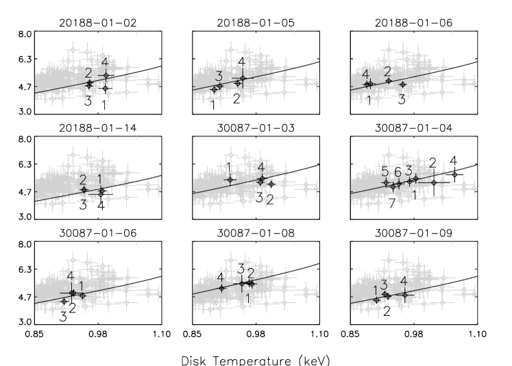
Figure 9: The obscured inner disk model, fitted to all of the chopped archival observations containing more than three sub-intervals. Observation numbers are listed in the upper left corner of each plot. Black points represent the chopped observations, while gray points represent our data. The solid black line plots the obscured inner disk model, which has been normalized to fit the chopped observations.

Why, in fact, does LMC X–3 have less apparent inner disk obscuration than LMC X–1 does? We can imagine at least three possible answers. The first option is that the coronal optical depth is much larger, in general, in LMC X–1 than in LMC X–3. This possibility is ruled out by the overlap between the two sources in terms of the flux ratio between the disk and power-law components; when the disk luminosity in LMC X–3 (catalog )is in decline, a significant power-law tail can form in that system without disrupting the excellent Stefan-Boltzmann relation for the disk component (Smith et al., 2007). A second possible answer supposes that the geometries of the coronae are very different: LMC X-3 has a geometrically large corona, while LMC X–1 has one that is more centrally concentrated, so that it obscures more of the inner disk while producing the same amount of upscattering. A third possibility supposes that the corona in both cases has a conelike shape (possibly a jet, but not necessarily, from our evidence alone), and that the apparent differences between the two sources are due to an inclination effect. In LMC X–1 (catalog ), which has an inclination of $36.38\pm 1.92^{\circ}$ (Orosz et al., 2009), the conical corona may block the inner parts of the disk as we look down through it, while in LMC X–3, with an inclination between $50^{\circ}$ and $70^{\circ}$ (van der Klis et al., 1985), the cone presents itself in semi-profile, where it doesn’t obscure the inner disk but we can still see the Compton upscattered flux it produces coming out its sides.

While either of the latter two pictures is consistent with our data, the last is more appealing for two reasons. Firstly, it does not require an unexplained difference in the form of the corona in the two binaries. Secondly, it may someday be possible to verify or to disprove using x-ray polarization observations. A ’down the barrel’ jet observation (e.g. LMC X–1) would sport a lower over-all scattering polarization fraction than an observation of the same type of geometry viewed ’in profile’ (e.g. LMC X–3) would. The precise magnitude of the expected polarization fraction difference will govern how easily its presence or absence can be verified. In any case, future observations with the GEMS x-ray polarimeter will at least begin to explore the relevant parameter space, provided the instrument can spend upwards of $10^{5}$ seconds observing each source (Jahoda, 2010).

Finally, we turn to the question of how a population of energetic electrons forms and dissipates above the innermost region of the disk on timescales shorter than $t_{visc}$. Figure 10 illustrates one possible accretion scenario that could account for LMC X–1’s unusual properties.

In this picture, the incoming wind material sheds its net angular momentum in the “post shock” before accreting onto the black hole (Hoyle & Lyttleton, 1939). Most of the shocked gas remains in the disk plane, and enters the accretion disk (middle arrow). A smaller portion of the heated post-shock matter launches on randomly distributed radial trajectories towards the black hole (upper and lower arrows). This component of the accretion flow rapidly heats on its radial descent into the black hole’s gravitational potential well. Unlike the disk, which is dense enough to cool efficiently via bremsstrahlung, the diffuse infalling matter cannot efficiently cool via free-free interactions. By the time the radially accreting matter passes over the inner disk, it can have reached electron temperatures above the $100$ keV required for the observed inverse Compton upscattering (Narayan & Yi, 1995; Ichimaru, 1977; Rees et al., 1982; Esin et al., 1998). This model allows the corona to change independently of the disk.

The presence of two accretion flow components, which are largely independent beyond the post-shock, is consistent with the constant observed total photon number and minimal disk luminosity variation in LMC X–1 (catalog ). Changes in the wind mass flux, due perhaps to wind clumping, register immediately in the radial, coronal flow. Viscous diffusion in the disk, meanwhile, smooths out those same sharp mass discontinuities. While the coronal surface density, and therefore the total energy of coronal emission changes rapidly, the disk emission evolves more slowly and less dramatically. The scenario of independent flows with the thin disk remaining intact beneath the corona, even when the latter is optically thick, is consistent with the picture derived from observations of the hard state and hard-to-soft transitions in 1E 1740.7-2942 and GRS 1758-258 (Smith et al., 2002). Recent observations of the iron fluorescence line in black holes in the hard state have shown relativistic line profiles indicating that the inner disk remains present even in the hard state (Miller et al., 2006), until extremely low lumniosities, below 1% of Eddington, are reached (Tomsick et al., 2009). In the luminosity range of LMC X–1, we therefore expect the inner disk to remain present, whether the thin disk is actually continuous or whether its inner portion is recondensed from a disk that is disrupted at intermediate radii (Liu et al., 2011).

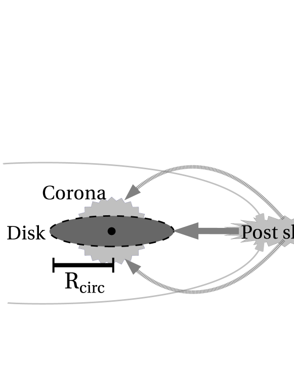
Figure 10: A cartoon of the accretion geometry of wind accretion systems. Incoming material from the companion’s wind (dashed gray lines) must dissipate its angular momentum in a shock front behind the compact object, a.k.a. the ’post shock’, before it can be accreted (thick arrow).

Differing patterns of x-ray variability (e.g. Figure 5) show promise as a means of identifying black hole companions when optical observations cannot. Fast changes in the inner disk temperature (Figure 5), and an anomalous temperature/luminosity relation (Figure 4), both combined with a stable net photon flux (Figure 7), may signal the presence of a wind accretor, perhaps combined with a low inclination, just as long-term hysteresis in state changes appears to be a signature of Roche-lobe overflow accretion and a large disk (Smith et al., 2002, 2007).

The type of two-component accretion flow proposed in this paper is best suited to black hole binary systems where the companion drives a high-velocity stellar wind. At the same time, this particular model leaves ample room for other coronal generation mechanisms that have already been proposed for black hole binary systems accreting via Roche-lobe overflow.

At least two types of observations can either help to confirm or to disprove the hypothesis we have proposed. The first focuses on recent x-ray observations of IC 10 X–1 and NGC 300 X–1 (Barnard et al., 2008). Both systems have disk to power-law luminosity ratios, as well as high-mass main-sequence companions, that resemble LMC X–1 (catalog )’s. Binary systems that contain both an O-type star capable of driving such a wind and a black hole companion are rare, which has made this particular combination of accretion mechanisms particularly hard to observe. Further observations of IC 10 X–1 and NGC 300 X–1, however, can potentially determine how deep their apparent similarities to LMC X–1 (catalog ) run, and will provide more opportunities to test our model’s veracity. The second test relies on observations of intermediate state, low-disk-fraction black hole binaries. These systems exhibit unusual temperature-luminosity relations akin to the ones seen in LMC X–1 (catalog ) (Dunn et al., 2011). One can confirm whether the same mechanism is at work in both LMC X–1 (catalog ) and an intermediate state system by measuring the variability (or lack thereof) of the latter’s total photon flux. Stable photon fluxes would support the proposition that these systems also contain stable, but variably-occulted, inner disks.

LMC X–1 (catalog ) has provided specific evidence that stellar mass black hole binaries may have x-ray spectral features which are unique to wind accretion. In a more general sense, the fact that LMC X–1 (catalog ) shares certain x-ray spectral properties with other types of black hole binary systems motivates further investigation of its seemingly unorthodox accretion mechanism’s full scope and utility.

References

- Agrawal et al. (1972) Agrawal, P. C., Gokhale, G. S., Iyengar, V. S., Kunte, P. K., Manchanda, R. K., & Sreekantan, B. V. 1972, Ap&SS, 18, 408
- Arnaud (1996) Arnaud, K. A. 1996, Astronomical Society of the Pacific Conference Series, Vol. 101, XSPEC: The First Ten Years, ed. G. H. Jacoby & J. Barnes, 17–+
- Baity et al. (1973) Baity, W. A., Ulmer, M. P., Wheaton, W. A., & Peterson, L. E. 1973, Nature, 245, 90
- Barnard et al. (2008) Barnard, R., Clark, J. S., & Kolb, U. C. 2008, A&A, 488, 697
- Belloni et al. (2000) Belloni, T., Migliari, S., & Fender, R. P. 2000, A&A, 358, L29
- Bolton (1972) Bolton, C. T. 1972, Nature, 235, 271
- Castor et al. (1975) Castor, J. I., Abbott, D. C., & Klein, R. I. 1975, ApJ, 195, 157
- Cowley et al. (1995) Cowley, A. P., Schmidtke, P. C., Anderson, A. L., & McGrath, T. K. 1995, PASP, 107, 145
- Davis & Hartmann (1983) Davis, R., & Hartmann, L. 1983, ApJ, 270, 671
- di Benedetto (1997) di Benedetto, G. P. 1997, ApJ, 486, 60
- Ducci et al. (2009) Ducci, L., Sidoli, L., Mereghetti, S., Paizis, A., & Romano, P. 2009, MNRAS, 398, 2152
- Dunn et al. (2010) Dunn, R. J. H., Fender, R. P., Körding, E. G., Belloni, T., & Cabanac, C. 2010, MNRAS, 403, 61
- Dunn et al. (2011) Dunn, R. J. H., Fender, R. P., Körding, E. G., Belloni, T., & Merloni, A. 2011, MNRAS, 411, 337
- Ebisawa et al. (1989) Ebisawa, K., Mitsuda, K., & Inoue, H. 1989, PASJ, 41, 519
- Esin et al. (1998) Esin, A. A., Narayan, R., Cui, W., Grove, J. E., & Zhang, S. 1998, ApJ, 505, 854
- Frank et al. (2002) Frank, J., King, A., & Raine, D. J. 2002, Accretion Power in Astrophysics: Third Edition, ed. Frank, J., King, A., & Raine, D. J.
- Gierliński et al. (2001) Gierliński, M., Maciołek-Niedźwiecki, A., & Ebisawa, K. 2001, MNRAS, 325, 1253
- Gierliński et al. (1999) Gierliński, M., Zdziarski, A. A., Poutanen, J., Coppi, P. S., Ebisawa, K., & Johnson, W. N. 1999, MNRAS, 309, 496
- Gou et al. (2009) Gou, L., et al. 2009, ApJ, 701, 1076
- Hanke et al. (2010) Hanke, M., Wilms, J., Nowak, M. A., Barragán, L., & Schulz, N. S. 2010, A&A, 509, L8+
- Heise et al. (1975) Heise, J., et al. 1975, Nature, 256, 107
- Herrero et al. (1995) Herrero, A., Kudritzki, R. P., Gabler, R., Vilchez, J. M., & Gabler, A. 1995, A&A, 297, 556
- Holt et al. (1975) Holt, S. S., Boldt, E. A., Kaluzienski, L. J., & Serlemitsos, P. J. 1975, Nature, 256, 108
- Holt et al. (1976) Holt, S. S., Kaluzienski, L. J., Boldt, E. A., & Serlemitsos, P. J. 1976, Nature, 261, 213
- Hoyle & Lyttleton (1939) Hoyle, F., & Lyttleton, R. A. 1939, in Proceedings of the Cambridge Philosophical Society, Vol. 35, Proceedings of the Cambridge Philosophical Society, 405–+
- Ichimaru (1977) Ichimaru, S. 1977, ApJ, 214, 840
- Jahoda (2010) Jahoda, K. 2010, in Presented at the Society of Photo-Optical Instrumentation Engineers (SPIE) Conference, Vol. 7732, Society of Photo-Optical Instrumentation Engineers (SPIE) Conference Series
- Jahoda et al. (2006) Jahoda, K., Markwardt, C. B., Radeva, Y., Rots, A. H., Stark, M. J., Swank, J. H., Strohmayer, T. E., & Zhang, W. 2006, ApJS, 163, 401
- King et al. (2007) King, A. R., Pringle, J. E., & Livio, M. 2007, MNRAS, 376, 1740
- Kudritzki & Puls (2000) Kudritzki, R., & Puls, J. 2000, ARA&A, 38, 613
- Kudritzki et al. (1989) Kudritzki, R. P., Pauldrach, A., Puls, J., & Abbott, D. C. 1989, A&A, 219, 205
- Lamers & Casinelli (1999) Lamers, H. J., & Casinelli, J. P. 1999, Introduction to Stellar Winds (Cambridge University Press)
- Levine & Corbet (2006) Levine, A. M., & Corbet, R. 2006, The Astronomer’s Telegram, 940, 1
- Liu et al. (2011) Liu, B. F., Done, C., & Taam, R. E. 2011, ApJ, 726, 10
- Miller et al. (2006) Miller, J. M., Homan, J., Steeghs, D., Rupen, M., Hunstead, R. W., Wijnands, R., Charles, P. A., & Fabian, A. C. 2006, ApJ, 653, 525
- Mitsuda et al. (1984) Mitsuda, K., et al. 1984, PASJ, 36, 741
- Narayan & Yi (1995) Narayan, R., & Yi, I. 1995, ApJ, 452, 710
- Nowak et al. (2001) Nowak, M. A., Wilms, J., Heindl, W. A., Pottschmidt, K., Dove, J. B., & Begelman, M. C. 2001, MNRAS, 320, 316
- Orosz et al. (2009) Orosz, J. A., et al. 2009, ApJ, 697, 573
- Owocki (1994) Owocki, S. P. 1994, Ap&SS, 221, 3
- Paczynski (1974) Paczynski, B. 1974, A&A, 34, 161
- Rees et al. (1982) Rees, M. J., Begelman, M. C., Blandford, R. D., & Phinney, E. S. 1982, Nature, 295, 17
- Sanford et al. (1975) Sanford, P. W., Ives, J. C., Bell Burnell, S. J., Mason, K. O., & Murdin, P. 1975, Nature, 256, 109
- Shapiro et al. (1976) Shapiro, S. L., Lightman, A. P., & Eardley, D. M. 1976, ApJ, 204, 187
- Smith et al. (2007) Smith, D. M., Dawson, D. M., & Swank, J. H. 2007, ApJ, 669, 1138
- Smith et al. (2002) Smith, D. M., Heindl, W. A., & Swank, J. H. 2002, ApJ, 569, 362
- Soria et al. (2001) Soria, R., Wu, K., Page, M. J., & Sakelliou, I. 2001, A&A, 365, L273
- Steiner et al. (2009) Steiner, J. F., Narayan, R., McClintock, J. E., & Ebisawa, K. 2009, PASP, 121, 1279
- Tomsick et al. (2009) Tomsick, J. A., Yamaoka, K., Corbel, S., Kaaret, P., Kalemci, E., & Migliari, S. 2009, ApJ, 707, L87
- van der Klis et al. (1985) van der Klis, M., Clausen, J. V., Jensen, K., Tjemkes, S., & van Paradijs, J. 1985, A&A, 151, 322
- Wilms et al. (2001) Wilms, J., Nowak, M. A., Pottschmidt, K., Heindl, W. A., Dove, J. B., & Begelman, M. C. 2001, MNRAS, 320, 327
- Yao et al. (2005) Yao, Y., Wang, Q. D., & Nan Zhang, S. 2005, MNRAS, 362, 229
- Ziółkowski (2005) Ziółkowski, J. 2005, MNRAS, 358, 851