2MASS wide field extinction maps: IV. The Orion, Mon R2, Rosette, and Canis Major star forming regions

We present a near-infrared extinction map of a large region (approximately $2\,200\mbox{ deg}^{2}$) covering the Orion, the Monoceros R2, the Rosette, and the Canis Major molecular clouds. We used robust and optimal methods to map the dust column density in the near-infrared (Nicer and Nicest) towards $\sim 19$ million stars of the Two Micron All Sky Survey (2MASS) point source catalog. Over the relevant regions of the field, we reached a 1-$\sigma$ error of $0.03\mbox{ mag}$ in the $K$-band extinction with a resolution of $3\mbox{ arcmin}$. We measured the cloud distances by comparing the observed density of foreground stars with the prediction of galactic models, thus obtaining $d_{\mathrm{OrionA}}=(371\pm 10)\mbox{ pc}$, $d_{\mathrm{OrionB}}=(398\pm 12)\mbox{ pc}$, $d_{\mathrm{MonR2}}=(905\pm 37)\mbox{ pc}$, $d_{\mathrm{Rosette}}=(1330\pm 48)\mbox{ pc}$, and $d_{\mathrm{CMa}}=(1150\pm 64)\mbox{ pc}$, values that compare very well with independent estimates.

1 Introduction

In a series of papers, we have applied an optimized multi-band technique dubbed Near-Infrared Color Excess Revisited (Nicer Lombardi & Alves, 2001, hereafter Paper 0) to measure dust extinction and investigate the structure of nearby molecular dark clouds using the Two Micron All Sky Survey (2MASS; Kleinmann et al., 1994). The main aim of our coordinated study is to investigate the large-scale structure of these objects and to clarify the link between the global physical properties of molecular clouds and their ability to form stars. Previously, we considered the Pipe nebula (see Lombardi et al., 2006, hereafter Paper I), the Ophiuchus and Lupus complexes (Lombardi et al., 2008, hereafter Paper II), and the Taurus, Perseus, and California complexes (Lombardi et al., 2010, hereafter Paper III). We now present an analysis of a large region covering more than $2\,200$ square degrees, centered around Orion. This region includes Orion A and B, $\lambda$ Orionis, Mon R2, Rosette, and Canis Major. An overview of a subset of the wide field extinction map presented in this paper, superimposed on an optical image of the sky, is presented in Fig. 1.

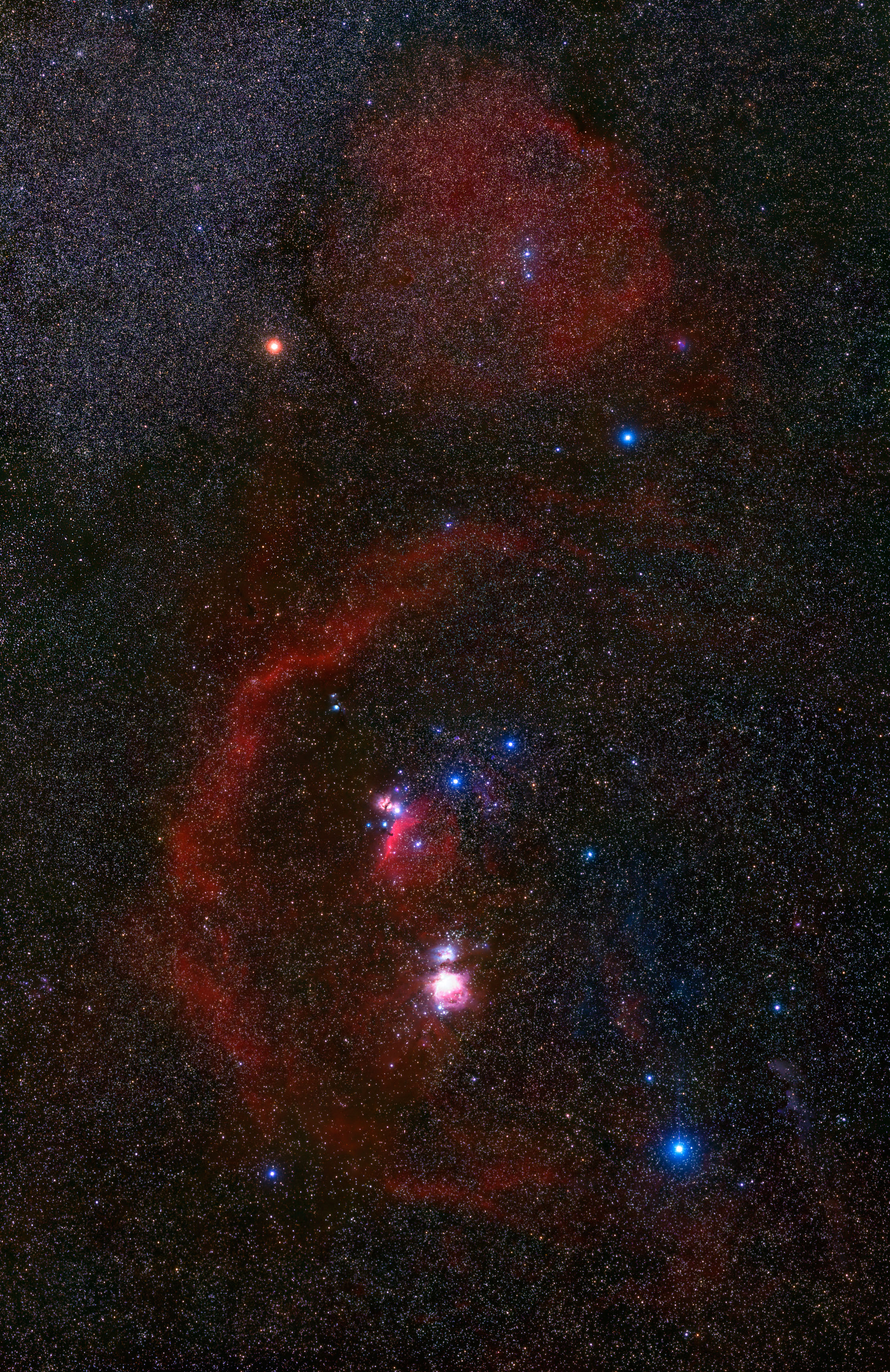
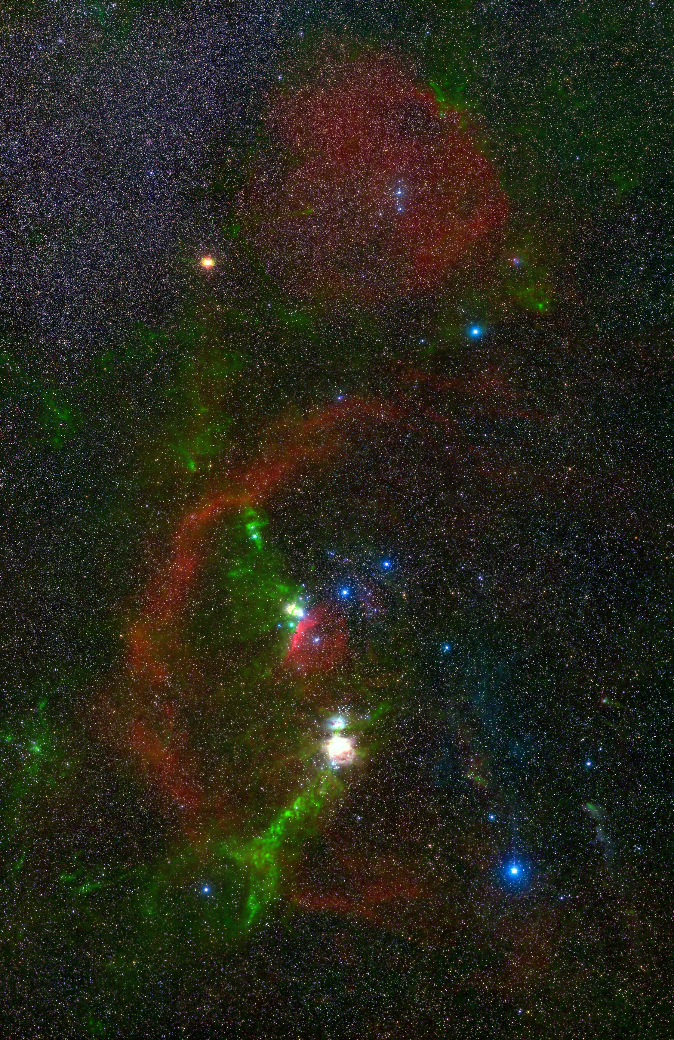
clouds11labels21

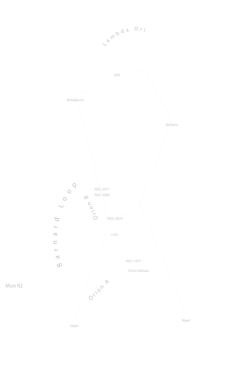
Figure 1: An optical image of Orion (Wei-Hao Wang, IfA, University of Hawaii) with the extinction map presented in this paper superimposed in green. The complementarity between the red Hii regions and the green $\mathrm{H}_{2}$ ones is evident. Note that the online figure is interactive: user /Subtype /Link /Border [0 0 0]/A ¡¡ /S/JavaScript /JS ( var aOCGs = this.getOCGs(); var AllChecked = 1; var AllIndex = 0; for(var i=0; aOCGs & i¡aOCGs.length;i++) if(aOCGs[i].name == ”clouds”) aOCGs[i].state = !aOCGs[i].state; if(!aOCGs[i].state aOCGs[i].name != ”all”) AllChecked = 0; if(aOCGs[i].name == ”all”) aOCGs[i].state = false; AllIndex=i; if(AllChecked == 1) aOCGs[AllIndex].state = true; ) ¿¿ extinction and user /Subtype /Link /Border [0 0 0]/A ¡¡ /S/JavaScript /JS ( var aOCGs = this.getOCGs(); var AllChecked = 1; var AllIndex = 0; for(var i=0; aOCGs & i¡aOCGs.length;i++) if(aOCGs[i].name == ”labels”) aOCGs[i].state = !aOCGs[i].state; if(!aOCGs[i].state aOCGs[i].name != ”all”) AllChecked = 0; if(aOCGs[i].name == ”all”) aOCGs[i].state = false; AllIndex=i; if(AllChecked == 1) aOCGs[AllIndex].state = true; ) ¿¿ labels can be toggled by clicking on the respective boxes when using Adobe^® Acrobat^®.

Near-infrared dust extinction measurement techniques present several advantages with respect to other column density tracers. As shown by Goodman et al. (2009), observations of dust are a better column density tracer than observations of molecular gas (CO), and observations of dust extinction in particular provide more robust measurements of column density than observations of dust emission, mainly because of the dependence of the latter measurements on uncertain knowledge of dust temperatures and emissivities. Additionally, the sensitivity reached by near-infrared dust extinction techniques, and by Nicer in particular, is essential to investigate the low-density regions of molecular clouds (which are often below the column density threshold required for the detection of the CO molecule) and therefore to estimate the mass of the diffuse gas that acts as a pressure boundary around the clumps. Similar to Paper III, we use for some key analyses in this paper the improved Nicest method (Lombardi, 2009), designed to cope better with the unresolved inhomogeneities present in the high-column density regions of the maps.

Orion is probably the best studied molecular cloud in the sky. The complex comprises Hii and Hi regions superimposed on colder, massive H₂ clouds with active formation of both low and high mass stars. The area studied here contains the Orion OB association, which is split in several subgroups with ages from $2$ to $12\mbox{ Myr}$. It is estimated that in the last $12\mbox{ Myr}$ there have been 10 to 20 supernovæ explosions (Bally, 2008) that shaped the gas in the region. More than a century ago, Barnard discovered a large arc of H_α emission around the eastern part of Orion (see Fig. 1). More recently, Barnard’s loop has been linked to Eridanus loop, and the two have been identified as a superbubble that is expanding into denser regions with a mean velocity of $10$–$20\mbox{ km s}^{-1}$ (Mac Low & McCray, 1988). Orion includes two giant molecular molecular clouds, Orion A and Orion B, the spectacular $\lambda$ Orionis bubble, and a large number of smaller cometary clouds. Both Orion A and B are observed in projection inside Barnard’s loop and most likely have been shaped by the supernova explosions, stellar winds, and Hii regions generated by OB stars in the area; for example, note the shell originating from the south-east extremity of Orion A, around the early B star $\kappa$ Orionis (Saiph). Orion A and B host rich clusters of young ($\sim 2\mbox{ Myr}$) stars, the Orion Nebula Cluster (ONC), NGC 2024 (also known as the Flame Nebula), NGC 2071, and NGC 2068. Just southwest of NGC 2024 is the famous Horsehead Nebula clearly visible as a protrusion of the green extinction map in Fig. 1.

Around the “head” of Orion, the O8 star $\lambda$ Orionis, there is a ring of dark clouds, $60\mbox{ pc}$ diameter, known for almost a century. The region hosts several young stars (including 11 OB stars very close to $\lambda$ Orionis), and their spatial and age distributions show that originally star formation occurred in an elongated giant molecular cloud (Mathieu, 2008; Duerr et al., 1982). Most likely, the explosion of a supernova coupled with stellar winds and Hii regions destroyed the dense central core, created an ionized bubble and a molecular shell visible as a ring. Star formation still continues in remnant dark clouds distant from the original core.

The Monoceros R2 region is distinguished by a chain of reflection nebulæ that extend over $2^{\circ}$ on the sky. The nomenclature “Mon R2” indicates the second association of reflection nebulæ in the constellation Monoceros van den Bergh (1966). The region is also well known for its dark nebula, which is clearly visible on top of the reflection nebulæ and the field stars. Clusters of newly formed stars are present in its core and in the GGD 12-15 region; smaller cores are also present in the field. The cloud is estimated to be at a distance significantly higher than the Orion nebula, $830\pm 50\mbox{ pc}$ (Herbst & Racine, 1976).

Rosette is known to amateur astronomers as one of the most spectacular nebulæ in the sky. The region is characterized by an expanding Hii region interacting with a giant molecular cloud. The Hii region has been photodissociated by NGC 2244, a cluster containing more than 30 high-mass OB stars. Judging from the age of NGC 2244, the Rosette molecular cloud has been actively forming stars for the last 2 to 3 Myr, and most likely will continue doing so, as there is still sufficient molecular material placed in a heavily stimulated environment (Román-Zúñiga & Lada, 2008). The distance to NGC 2244, and therefore to the molecular cloud, is still controversial: recent estimates range between $1\,390\mbox{ pc}$ (Hensberge et al., 2000) and $1\,670\mbox{ pc}$ (Park & Sung, 2002).

The star-forming region in Canis Major is characterized by a concentrated group of early type stars (forming the CMa OB1/R1 associations) and by an arc-shaped molecular cloud (probably produced by a supernova explosion). Similarly to Rosette, Canis Major presents an interface between the Hii region and the neutral gas which shows up as a north-south oriented ridge. Recent distance determinations of Canis Major seem to converge around a distance of $1\,000\mbox{ pc}$ (Gregorio-Hetem, 2008).

This paper is organized as follows. In Sect. 2 we briefly describe the technique used to map the dust and we present the main results obtained. Section 3 is devoted to an in-depth statistical analysis, and includes a discussion of the measured reddening laws for the various clouds, the measurements of the distances using foreground stars, the log-normality of the column density distributions, and the effects of small-scale inhomogeneities. The mass estimates for the clouds are presented in Sect. 4. Finally, we summarize the results obtained in Sect. 5.

A few plots in this paper are associated with switches designed to show or hide labels; these are shown as frames in the respective captions. In order to use this feature this electronic document should be displayed using Adobe^® Acrobat^®.

2 NICER and NICEST extinction maps

The data analysis was carried out following the technique presented in Paper 0 and used also in the previous papers of this series, to which we refer for the details (see in particular Paper III). We selected reliable point source detections from the Two Micron All Sky Survey (2MASS; Kleinmann et al., 1994) in the region

$$180^{\circ}<{} l<240^{\circ}\;, -40^{\circ}<{} b<0^{\circ}\;.$$ (1)

This area is $\sim 2\,200$ square degrees and contains approximately $19$ million point sources from the 2MASS catalog. The region encloses many known dark molecular cloud complexes, including the Orion and Mon R2 star forming regions, the $\lambda$ Orionis bubble, the Rosette nebula, and the Canis Major complex (see Fig. 3).

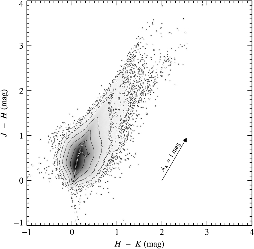
Figure 2: Color-color diagram of the stars in the whole field. The contours are logarithmically spaced, with each contour representing a density ten times larger than the enclosing contour; the outer contour detects single stars. Only stars with accurate photometry in all bands (maximum 1-$\sigma$ errors allowed $0.1\mbox{ mag}$) have been included in this plot. The diagonal spread of stars is due to reddening along the marked reddening vector of dwarf and giant stars. The expected colors of these stars, as predicted by Bessell & Brett (1988) and converted into the 2MASS photometric system using the relations from (Carpenter, 2001), are shown in the plot, and match very well the observed colors.

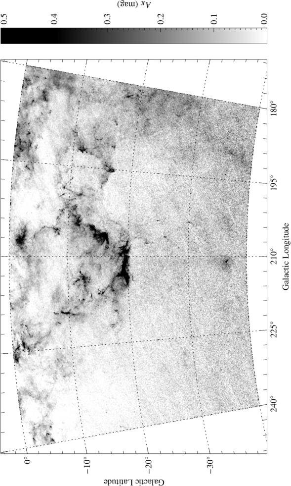
fig331

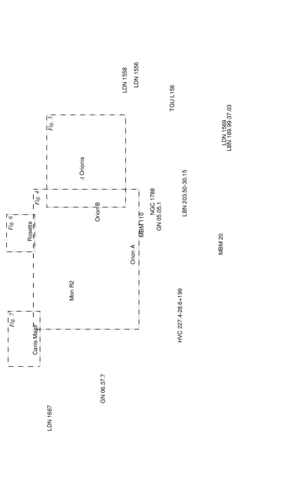
Figure 3: The Nicer extinction map of the Orion, Mon R2, Rosette, and Canis Major complexes. The resolution is $\mathrm{FWHM}=3\mbox{ arcmin}$. The various dashed boxes mark the regions shown in greater detail in Figs. 4–7. Toggle user /Subtype /Link /Border [0 0 0]/A ¡¡ /S/JavaScript /JS ( var aOCGs = this.getOCGs(); var AllChecked = 1; var AllIndex = 0; for(var i=0; aOCGs & i¡aOCGs.length;i++) if(aOCGs[i].name == ”fig3”) aOCGs[i].state = !aOCGs[i].state; if(!aOCGs[i].state aOCGs[i].name != ”all”) AllChecked = 0; if(aOCGs[i].name == ”all”) aOCGs[i].state = false; AllIndex=i; if(AllChecked == 1) aOCGs[AllIndex].state = true; ) ¿¿ labels.

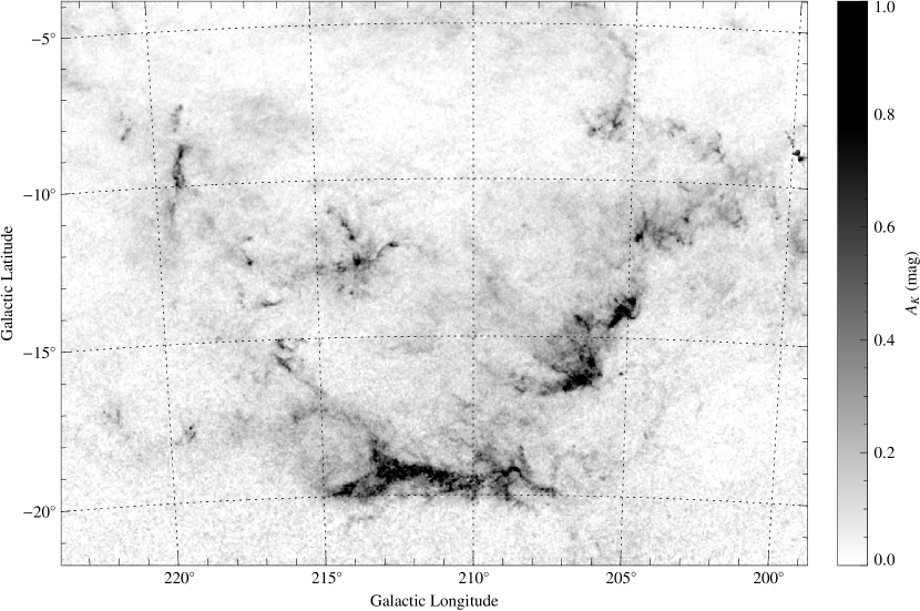
fig4a41

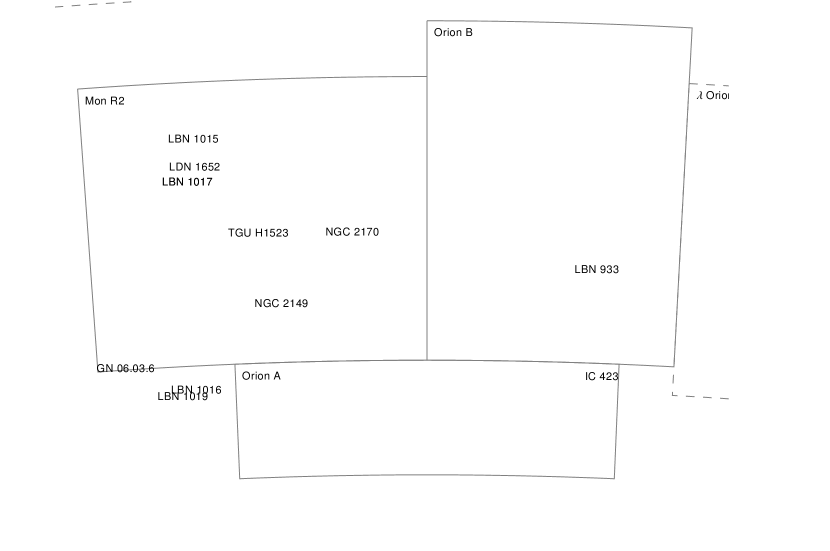
Figure 4: A zoom of Fig. 3 showing the Orion A (bottom), Orion B (top right), and Mon R2 (top left) star forming regions. The several well studied objects are marked. The artifacts around $l=200^{\circ}$ and $b=-9^{\circ}$ are caused by Betelgeuse. Toggle user /Subtype /Link /Border [0 0 0]/A ¡¡ /S/JavaScript /JS ( var aOCGs = this.getOCGs(); var AllChecked = 1; var AllIndex = 0; for(var i=0; aOCGs & i¡aOCGs.length;i++) if(aOCGs[i].name == ”fig4a”) aOCGs[i].state = !aOCGs[i].state; if(!aOCGs[i].state aOCGs[i].name != ”all”) AllChecked = 0; if(aOCGs[i].name == ”all”) aOCGs[i].state = false; AllIndex=i; if(AllChecked == 1) aOCGs[AllIndex].state = true; ) ¿¿ labels.

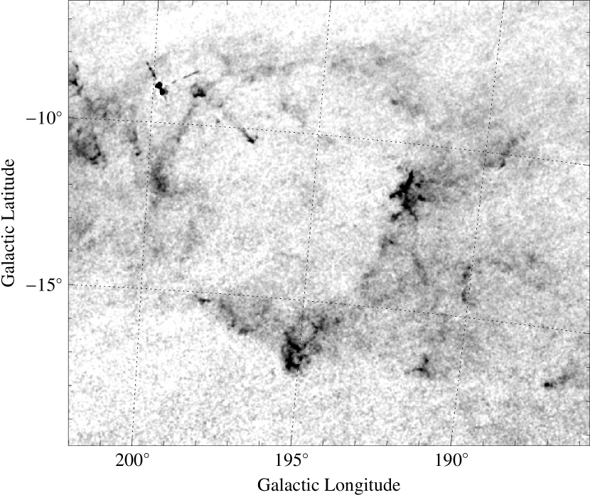
fig4b51

Figure 5: A zoom of Fig. 3 showing the $\lambda$ Orionis bubble. Toggle user /Subtype /Link /Border [0 0 0]/A ¡¡ /S/JavaScript /JS ( var aOCGs = this.getOCGs(); var AllChecked = 1; var AllIndex = 0; for(var i=0; aOCGs & i¡aOCGs.length;i++) if(aOCGs[i].name == ”fig4b”) aOCGs[i].state = !aOCGs[i].state; if(!aOCGs[i].state aOCGs[i].name != ”all”) AllChecked = 0; if(aOCGs[i].name == ”all”) aOCGs[i].state = false; AllIndex=i; if(AllChecked == 1) aOCGs[AllIndex].state = true; ) ¿¿ labels.

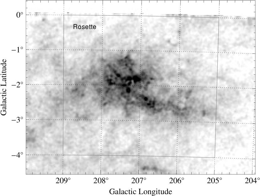
Figure 6: A zoom of Fig. 3 showing the Rosette complex.

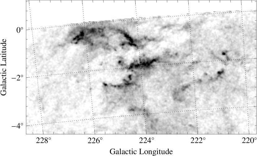
fig4d61

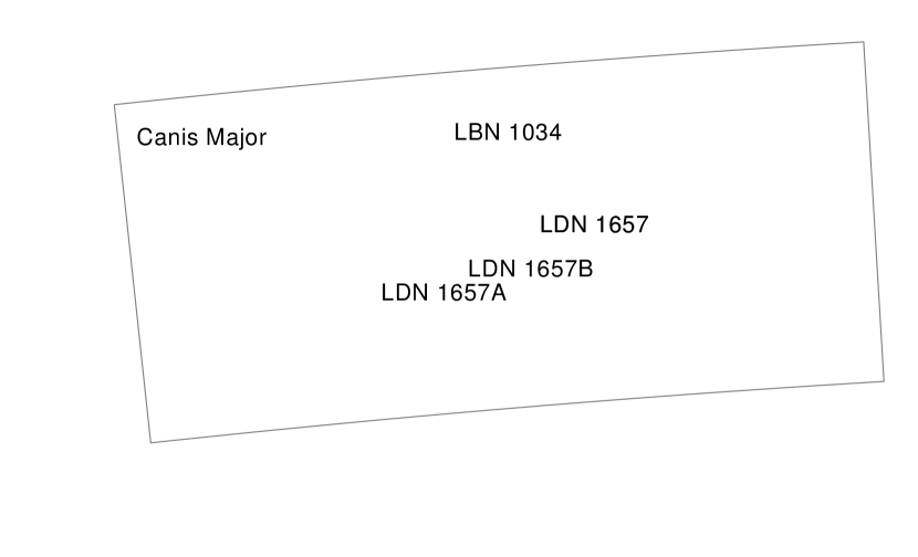
Figure 7: A zoom of Fig. 3 showing the Canis Major dark complex. Toggle user /Subtype /Link /Border [0 0 0]/A ¡¡ /S/JavaScript /JS ( var aOCGs = this.getOCGs(); var AllChecked = 1; var AllIndex = 0; for(var i=0; aOCGs & i¡aOCGs.length;i++) if(aOCGs[i].name == ”fig4d”) aOCGs[i].state = !aOCGs[i].state; if(!aOCGs[i].state aOCGs[i].name != ”all”) AllChecked = 0; if(aOCGs[i].name == ”all”) aOCGs[i].state = false; AllIndex=i; if(AllChecked == 1) aOCGs[AllIndex].state = true; ) ¿¿ labels.

As a preliminary step, we constructed the color-color diagram of the stars to check for the possible presence of anomalies in colors of stars. The result, shown in Fig. 2, displays a weak sign of bifurcation in the distribution of source colors along the reddening vector. This is likely to be due to the different colors of extinguished field stars and Asymptotic Giant Branch (AGB) stars. However, given the weakness of the AGB stars contamination, we decided to proceed similarly to Paper III and not exclude any object.

After the selection of a control field for the calibration of the intrinsic colors of stars (and their covariance matrix) we produced the final 2MASS/Nicer extinction map, shown in Fig. 3. To obtain these results, we smoothed the individual extinctions measured for each star, $\bigl{\{}\hat{A}^{(n)}_{K}\bigr{\}}$, using a moving weighted average

$$\hat{A}_{K}(\@vec{\theta})=\frac{\sum_{n=1}^{N}W^{(n)}(\@vec{\theta})\hat{A}^{(n)}_{K}}{\sum_{n=1}^{N}W^{(n)}(\@vec{\theta})}\;,$$ (2)

where $\hat{A}_{K}(\@vec{\theta})$ is the extinction at the angular position $\@vec{\theta}$ and $W^{(n)}(\@vec{\theta})$ is the weight for the $n$-th star for the pixel at the location $\@vec{\theta}$. This weight, in the standard Nicer algorithm, is a combination of a smoothing, window function $W\bigl{(}\@vec{\theta}-\@vec{\theta}^{(n)}\bigr{)}$, i.e. a function of the angular distance between the star and the point $\@vec{\theta}$ where the extinction has to be interpolated, and the inverse of the inferred variance on the estimate of $A_{K}$ from the star:

$$W^{(n)}(\@vec{\theta})=\frac{W\bigl{(}\@vec{\theta}-\@vec{\theta}^{(n)}\bigr{)}}{\mathrm{Var}\bigl{(}\hat{A}^{(n)}_{K}\bigr{)}}\;.$$ (3)

Note that the way Eq. (2) is written, only relative values of $W^{(n)}$, and thus of $W\bigl{(}\@vec{\theta}-\@vec{\theta}^{(n)}\bigr{)}$ are important. Therefore, we can assume without loss of generality that the window function is normalized to unity according to the equation

$$\int W(\@vec{\theta})\,\mathrm{d}^{2}\theta=1\;.$$ (4)

For this paper, the smoothing window function $W$ was taken to be a Gaussian with $\mathit{FWHM}=3\mbox{ arcmin}$. Finally, the map described by Eq. (2) was sampled at $1.5\mbox{ arcmin}$ (corresponding to a Nyquist frequency for the chosen window function).

Similarly to Paper III, we also constructed a Nicest extinction map, obtained by using the modified estimator described in Lombardi (2009). The Nicest map differs significantly from the Nicer map only in the high column-density regions, where the substructures present in the molecular cloud produce a possibly significant bias on the standard estimate of the column density (see below). The largest extinction was measured close to LDN 1641 S, where $A_{K}\simeq 2.0\mbox{ mag}$ for Nicer and $A_{K}\simeq 5.0\mbox{ mag}$ for Nicest.

Figures 4–7 show in greater detail the absorption maps we obtained for the Orion and Mon R2 star forming regions, the $\lambda$ Orionis bubble, the Rosette nebula, and the Canis Major complex. These maps allow us to better appreciate the details that we can obtain by applying the Nicer method to the 2MASS data. In the figures we also display the boundaries that we use throughout this paper and that we associate with the various clouds considered here. In particular, we defined

Orion A: $$203^{\circ}\leq l {}\leq 217^{\circ}\;, -21^{\circ}\leq b {}\leq-17^{\circ}\;,$$

Orion B: $$201^{\circ}\leq l {}\leq 210^{\circ}\;, -17^{\circ}\leq b {}\leq-5^{\circ}\;,$$

Mon R2: $$210^{\circ}\leq l {}\leq 222^{\circ}\;, -17^{\circ}\leq b {}\leq-7^{\circ}\;,$$

$$\lambda 188^{\circ}\leq l {}\leq 201^{\circ}\;, -18^{\circ}\leq b {}\leq-7^{\circ}\;,$$ Orionis:

Rosette: $$205^{\circ}\leq l {}\leq 209^{\circ}\;, -4^{\circ}\leq b {}\leq 0^{\circ}\;,$$

Canis Major: $$220^{\circ}\leq l {}\leq 228^{\circ}\;, -4^{\circ}\leq b {}\leq 0^{\circ}\;.$$ (5)

We note that the boundaries defined are somewhat arbitrary, but as described below (see Sect. 3.2 and in particular Fig. 9) there are strong indications that many (if not all) of the features within each of the defined regions are located at similar distances. We stress in any case that some of the results presented (for example, the mass estimates discussed in Sect. 4) depend significantly on the chosen boundaries.

The expected error on the measured extinction, $\sigma_{\hat{A}_{K}}$ (not shown here), was evaluated from a standard error propagation in Eq. (2) [see below Eq. (9)]. The main factor affecting the error is the local density of stars, and thus there is a significant change in the statistical error along galactic latitude. Other variations can be associated with bright stars (which are masked out in the 2MASS release), bright galaxies, and to the cloud itself. The median error per pixel for the field shown in Fig. 4 is $0.029\mbox{ mag}$, while a significantly lower error of $0.019\mbox{ mag}$ is observed for the Rosette or Canis Major nebulæ.

3 Statistical analysis

3.1 Reddening law

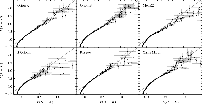
Figure 8: The reddening law as measured on various complexes. The plots show the color excess on $J-H$ as a function of the color excess on $H-K$. Error bars are uncertainties evaluated from the photometric errors of the 2MASS catalog and taking into account also the intrinsic scatter in the individual colors of the stars, as derived from the control field. The solid line shows the normal infrared reddening law (Indebetouw et al., 2005). A significant discrepancy is observed for Mon R2 and possibly for $\lambda$ Orionis, while other clouds are in very good agreement with the normal infrared reddening law.

As shown in Paper 0, the use of multiple colors in the Nicer algorithm significantly improves the signal-to-noise ratio of the final extinction maps, but also provides a simple, direct way to verify the reddening law. A good way to perform this check is to divide all stars with reliable measurements in all bands into different bins corresponding to the individual $\hat{A}_{K}^{(n)}$ measurements, and to evaluate the average NIR colors of the stars in the same bin. At first, this procedure might be regarded as a circular argument: in order to measure the extinction law one bins the colors of stars according to the estimated extinction! In reality, the method is well behaved and has interesting properties (Ascenso et al. 2011, in preparation):

• The assumed reddening law is only used to bin the data, and is then iteratively replaced by the new reddening law as determined from the data.

• This iterative process converges quickly and is essentially unbiased; the final reddening law essentially does not depend on the initial assumed one.

• Simulations show that more standard techniques (such as binning in one simple color, e.g. $J-K$) suffer from significant biases mostly as a result of the heteroskedasticity of the data; additional complications are due to the correlation of errors in the two colors $J-H$ and $H-K$.

Figures 8 summarize the results obtained for a bin size of $0.02\mbox{ mag}$ in the various clouds. As shown by these plots, in all clouds we have a good agreement between the standard Indebetouw et al. (2005) infrared reddening law in the 2MASS photometric system and the observed one. All plots show a systematic divergence below the reddening line at “negative” extinctions, an effect due to the intrinsic colors of dwarf stars (see Koornneef, 1983; Bessell & Brett, 1988). Specifically, the track of dwarf stars in the $J-H$ vs. $H-K$ color-color plot is slightly steeper than the reddening vector (cf. Fig. 2), and as a result stars in the bottom-left of the dwarf track, which in the simple Nicer scheme are associated to negative extinction, exhibit an excess in their $H-K$ color. This effect is not visible anymore as we go to positive extinction because the colors of these stars are then averaged together with the rest of the dwarf and giant sequence, and as imposed by the control field no systematic color excesses is present.

Another common feature to all plots of Fig. 8 is an increase in the spread of points in the upper-right corner, i.e. for high column densities. As shown by the correspondingly larger error bars, this is expected and is a result of the low number of stars showing large extinction values (we recall that a constant bin size of $0.02\mbox{ mag}$ has been used everywhere). Additionally, for some clouds, and in particular for Mon R2, we observe that the points fall systematically below the standard Indebetouw et al. (2005) reddening law. We believe that this difference is not due to intrinsic differences in the physical properties of the dust, but rather that it is caused by contamination from a population of relatively blue, young stars present in the field, both in the form of clusters and of dispersed OB associations (in particular, the area is known to host the Mon OB1 association, see Racine, 1968; Herbst & Racine, 1976; Carpenter & Hodapp, 2008).

Finally, we stress that the check performed with Fig. 8 is a relative one: we can only verify that slope of the reddening vector agrees with expectations from the standard Indebetouw et al. (2005) reddening law, but can not constrain the length of the reddening vector.

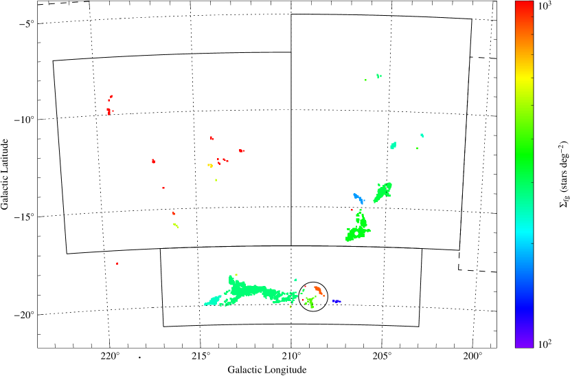
Figure 9: The local density of foreground stars, averaged on connected regions with extinction $A_{K}>0.6\mbox{ mag}$. The three regions defined in Fig. 4 are shown again here.

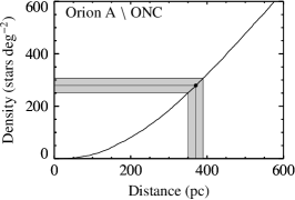
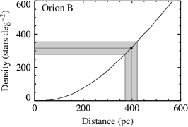
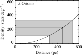
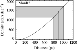
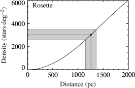
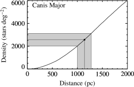
Figure 10: The distances of the clouds deduced from the density of foreground stars. Solid lines show the density of foreground of stars as a function of the cloud distance, as predicted from the Robin et al. (2003) Galactic model. The grey areas correspond to the $95\%$ (two-sigma) confidence regions for the density of foreground stars and the deduced confidence regions for the distances.

3.2 Foreground star contamination and distances

Foreground stars are an annoyance for color extinction studies, since they dilute the signal coming from background stars and add a source of noise to the maps. For nearby clouds, foreground stars are usually a small fraction of the total number of stars in all regions except in the very dense cores (where the density of background stars decreases significantly because of the dust extinction). In these conditions, one can safely ignore the bias introduced by foreground stars, and if necessary use Nicest measurements to alleviate the foreground bias in the high column-density regions.

Complex	$N_{\mathrm{fg}}$	$f$	Area	$\Sigma_{\mathrm{fg}}$	Distance
			$\mbox{deg}^{2}$	$\mbox{deg}^{-2}$	pc
Orion A	420	0.047	1.504	$\phantom{0}279\pm 13\phantom{0}$	$\phantom{0}371\pm 10$
Orion B	298	0.030	0.936	$\phantom{0}318\pm 18\phantom{0}$	$\phantom{0}398\pm 12$
$\lambda$ Orionis	017	0.018	0.078	$\phantom{0}219\pm 53\phantom{0}$	$\phantom{0}445\pm 50$
Mon R2	207	0.157	0.144	$1430\pm 99\phantom{0}$	$\phantom{0}905\pm 37$
Rosette	275	0.190	0.083	$3330\pm 200$	$1330\pm 48$
Canis Major	099	0.228	0.036	$2730\pm 270$	$1150\pm 64$

Table 1: The average value of foreground stars $N_{\mathrm{fg}}$ and their fraction $f$ found in the various complexes. Also reported in the last column the estimated distance from a comparison with the Robin et al. (2003) Galactic model (see Fig. 10).

Foreground stars are easily selected in the dense regions of a molecular cloud as objects showing no or very little sign of extinction. This allows us to estimate with good accuracy the local density of foreground stars in all high-column density clouds in our field. For this purpose, we selected connected regions with $\hat{A}_{K}(\@vec{\theta})>0.6\mbox{ mag}$ in our extinction map, and we computed for each of these the local density of foreground stars (foreground objects were selected as stars with K-band extinction smaller than $0.3\mbox{ mag}$, i.e. stars compatible with no or negligible extinction). Figure 9 shows the results obtained in Orion and Mon R2; the average numerical values obtained in the various regions considered in this paper are also reported in Table 1. Two simple results are immediately visible from Fig. 9. First, the Orion cloud shows significantly fewer foreground stars than the Mon R2 complex, as expected from the much larger distance assigned in the literature to Mon R2. Second, all complexes have relatively uniform densities of foreground stars in their regions except the area around the Orion Nebula Cluster (ONC), marked with a circle in Fig. 9. This result is also expected, since it is well known that the ONC region contains a high surface density of young stellar objects (YSOs) embedded in the cloud that will contaminate our extinction measurements and a part of which will be considered as foreground stars by our selection criteria. In order to obtain unbiased results, we excluded this region in the analysis of the foreground star density.

We note that a comparison of the densities reported in Table 1 with the average density of stars in the field, $\Sigma\sim 9\,000\mbox{ deg}^{-2}$, shows that the expected fraction $f$ of foreground stars in the outskirts of the Orion complex is expected to be as low as $f\simeq 0.04$, while a significantly larger value, $f\simeq 0.16$, is expected for Mon R2.

Interestingly, as shown in Paper III, we can also use foreground stars to estimate the distance of dark clouds. The technique relies on a comparison between the estimated density of foreground stars and the predictions of galactic models for the photometric depth of the 2MASS catalog. We used the Galactic model by Robin et al. (2003), and computed at the location of each cloud the expected number of stars within the 2MASS photometric limits observed at various distances (see Fig. 10). The results obtained, shown in the last column of Table 1, presents several interesting aspects. First, the estimates for the Orion A distance, when excluding the highly contaminated area of the ONC, is $(371\pm 10)\mbox{ pc}$. This value is considerably less than the “standard” Orion distance, $450\mbox{ pc}$, but as discussed by Muench et al. (2008), this often quoted distance is actually reported by Genzel & Stutzki (1989) but it is not itself the result of any direct measurement, but more likely an average of two different measurements. In general, in spite of the efforts over several decades to measure the distance of this cloud complex, there is still a spread in recent estimates at the $10\%$ level (Muench et al., 2008). We stress, however, that our measurement is in good agreement with a recent VLBI determination, $(389\pm 23)\mbox{ pc}$ (Sandstrom et al., 2007), but lower than a measurement by Menten et al. (2007), $(414\pm 7)\mbox{ pc}$.

Our Orion A distance is also very close to the Orion B distance, a result that is not unexpected given the physical relationship between the two clouds.

We did attempt a measurement of the $\lambda$ Orionis distance, in spite of the relative lack of dense material in the area. This paucity of high extinction material prevents us from estimating the density of foreground stars with the necessary confidence. Nonetheless, the result obtained is virtually identical to the standard distance estimated by Dolan & Mathieu (2001) using Stroömgren photometry of the OB stars in a main-sequence fitting in a theoretical H-R diagram, $450\pm 50\mbox{ pc}$. However, we are unfortunately unable to improve this result in terms of accuracy.

The Mon R2 cloud is found to be at a significantly larger distance, $(905\pm 37)\mbox{ pc}$, a result that compares well with the generally accepted distance of this cloud, $(830\pm 50)\mbox{ pc}$ (Herbst & Racine, 1976; see also Carpenter & Hodapp, 2008). We stress that, as evident from Fig. 9, different clouds present in the MonR2 region seem to have compatible surface densities of foreground stars and therefore distances, with the possible exception of the filaments close to NGC 2149. In order to test quantitatively this statement, we also considered subregions in the MonR2 cloud. In particular, a measurement of the distance of the LBN 1015, LDN 1652, and LBN 1017 clouds (the “crossbones”) provides $(750\pm 100)\mbox{ pc}$, while a measurement of the MonR2 core alone (i.e. the area around NGC 2170) gives $(925\pm 150)\mbox{ pc}$. These two regions therefore seem to be at comparable distances, a result that is in contradiction with what found by Wilson et al. (2005). Unfortunately, the data we have are not sufficient to constrain the distance of the filaments around NGC 2149, and therefore we cannot securely associate them with MonR2 (nor with Orion A).

The distance of the Rosette complex is generally obtained indirectly by measuring the distance of the NGC 2244 cluster. Typical values obtained from photometric studies are around $1650\mbox{ pc}$ (Johnson, 1962; Perez et al., 1987; Park & Sung, 2002), with the exception of Ogura & Ishida (1981) that reports $1420\mbox{ pc}$ (see also Román-Zúñiga & Lada, 2008 for a discussion of these measurements). Hensberge et al. (2000) performed a spectroscopic analysis of the binary member V578 Mon, obtaining $1390\mbox{ pc}$, a value that compares very well with our determination.

Recent distance estimates of the Canis Major region (and in particular of its OB association) are close to $1000\mbox{ pc}$ (see Gregorio-Hetem, 2008 and references therein). Although our measurement appears to be slightly higher, the uncertainties of the data present in the literature and of our own determination are relatively large.

In summary, our analysis shows that for clouds outside the reach of Hipparcos parallaxes, a model-dependent distance obtained through number counts of foreground stars is a reasonable alternative of distance determination. Indeed, for all clouds studied here we obtained results that are in very good agreement with the data present in the literature (which often are obtained using dedicated observations). Additionally, the uncertainty we have is generally comparable to the one that can be obtained with competitive techniques (with the notable exception of VLBI parallaxes, which however are very expensive in terms of telescope time and need to rely on a secure physical link between the source measured and the molecular cloud). The statistical error associated with this technique is linked to $N_{\mathrm{fg}}$, the number of foreground stars observed in projection to the cloud. This quantity, for nearby clouds, increases linearly with the cloud distance $d$, and therefore the relative statistical error on the estimated distance goes as $1/\sqrt{d}$.

3.3 Column density probability distribution

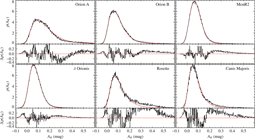
Figure 11: The probability distributions of pixel extinctions for the six cloud complexes. In each plot, the red, solid curve represents the best-fit with a log-normal distribution. Lower panels show the residuals with respect to the best-fit.

Table 2: The best-fit parameters of the four Gaussian functions used to fit the column density probability distribution shown in Figs. 11 (see Eq. (6) for the meaning of the various quantities).

Cloud	Offset $A_{0}$	Scale $A_{1}$	Dispersion $\sigma$
Orion A	$-0.059$	$0.193$	$0.491$
Orion B	$-0.060$	$0.145$	$0.482$
Mon R2	$-0.163$	$0.238$	$0.214$
$\lambda$ Orionis	$-0.053$	$0.121$	$0.378$
Rosette	$+0.027$	$0.079$	$1.167$
Canis Major	$+0.013$	$0.053$	$0.978$

Many theoretical studies have suggested that the turbulent supersonic motions that are believed to characterize the molecular clouds on large scales induce a log-normal probability distribution for the volume density (e.g. Vazquez-Semadeni, 1994; Padoan et al., 1997b; Passot & Vázquez-Semadeni, 1998; Scalo et al., 1998). Although this result strictly applies for the volume density, under certain assumptions, verified in relatively “thin” molecular clouds, the probability distribution for the column density, i.e. the volume density integrated along the line of sight, is also expected to follow a log-normal distribution (Vázquez-Semadeni & García, 2001). Additionally, Tassis et al. (2010) recently have shown that log-normal distributions are also expected under completely different physical conditions (also plausible for molecular clouds), such as radially stratified density distributions dominated by gravity and thermal pressure, or by a gravitationally-driven ambipolar diffusion.

The log-normality of the column densities is verified with good approximation at low-column densities in many of the clouds that we have studied in the past and by similar results obtained by Kainulainen et al. (2009), Goodman et al. (2009), and Froebrich & Rowles (2010). As shown by the plots in Fig. 11, the region studied here confirms this general trend. The probability distributions of column densities for the various clouds were fitted with a log-normal distributions of the form

$$h(A_{K})=\frac{a}{A_{K}-A_{0}}\exp\left[-\frac{\bigl{(}\ln(A_{K}-A_{0})-\ln A_{1}\bigr{)}^{2}}{2\sigma^{2}}\right]\;.$$ (6)

For some of the clouds, such as Orion B, $\lambda$ Orionis, and Mon R2, the fits appear to be better than for other ones, such as Orion A or Rosette. However, in all cases residuals are well above the expected levels and show systematic and structured deviations even at low column densities. Additionally, all clouds show a positive residual at the higher column densities, approximately for $A_{K}>0.2\mbox{ mag}$. The significance of these results and the goodness of the fits need to be further investigated.

One perhaps surprising feature of Fig. 11 is the presence of a significant number of column density estimates with negative values. This could be either due to a zero-point offset in the control field or to uncertainties in the column density measurements, which naturally broadens the intrinsic distribution and possibly adds a fraction of negative measurements. Note also that the amount of negative pixels observed is compatible with the typical error on our extinction maps, which is of the order of $0.03\mbox{ mag}$.

3.4 Small-scale inhomogeneities

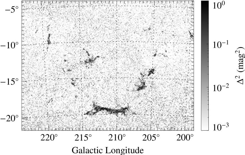
Figure 12: The $\Delta^{2}$ map of Eq. (7) on the same region shown in Fig. 4. Note the significant increase observed in $\Delta^{2}$ close to the central parts of this cloud.

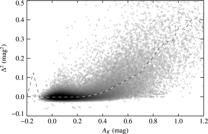
Figure 13: The distribution of the $\Delta^{2}$ map as a function of the local extinction $A_{K}$ for the map in Fig. 3, in logarithmic grey scale. The dashed line shows the average values of $\Delta^{2}$ in bins of $0.05\mbox{ mag}$ in $A_{K}$. Note the rapid increase of $\Delta^{2}$ for $A_{K}>0.7\mbox{ mag}$. As a comparison, the average variance $\mathrm{Var}\bigl{(}\hat{A}^{(n)}_{K}\bigr{)}$ on the estimate of $\hat{A}_{K}$ from a single star is approximately $0.033\mbox{ mag}^{2}$.

Lada et al. (1994) first recognized that the local dispersion of extinction measurements increases with the column density. In other words, within a single “pixel element,” the scatter of the individual stellar column density estimates is proportional to the average local column density estimate. This results implies the presence of substructures on scales smaller than the resolution of the extinction maps, and shows that theses substructures are more evident in regions with high column density. Substructures could be due either to unresolved gradients or to random fluctuations induced by turbulence (see Lada et al., 1999)

The presence of undetected inhomogeneities is important for two reasons: (i) they might contain signatures of turbulent motions (see, e.g. Miesch & Bally, 1994; Padoan et al., 1997a), and (ii) they are bound to bias the extinction measurements towards lower extinctions in high-column density regions (and, especially, in the very dense cores; see Lombardi, 2009).

In the previous papers of this series we have considered a quantity that traces well the inhomogeneities:

$$\Delta^{2}(\@vec{\theta})\equiv\hat{\sigma}^{2}_{\hat{A}_{K}}(\@vec{\theta})+\sigma^{2}_{\hat{A}_{K}}(\@vec{\theta})-\bigl{\langle}\mathrm{Var}\bigl{(}\hat{A}_{K}^{(n)}\bigr{)}\bigr{\rangle}(\@vec{\theta})\;.$$ (7)

The $\Delta^{2}$ map is defined in terms of the observed variance of column density estimates,

$$\hat{\sigma}^{2}_{\hat{A}_{K}}(\@vec{\theta})\equiv\frac{\sum_{n=1}^{N}W^{(n)}\bigl{[}\hat{A}_{K}^{(n)}-\hat{A}_{K}(\@vec{\theta})\bigr{]}^{2}}{\sum_{n=1}^{N}W^{(n)}}\;,$$ (8)

the average expected scatter due to the photometric errors and the intrinsic dispersion in the colors of the stars

$$\sigma^{2}_{\hat{A}_{K}}(\@vec{\theta})\equiv\frac{\sum_{n=1}^{N}\bigl{[}W^{(n)}(\@vec{\theta})\bigr{]}^{2}\mathrm{Var}\bigl{(}\hat{A}_{K}^{(n)}\bigr{)}}{\Bigl{[}\sum_{n=1}^{N}W^{(n)}(\@vec{\theta})\Bigr{]}^{2}}\;,$$ (9)

and of the weighted average expected variance for the column density measurements around $\@vec{\theta}$

$$\bigl{\langle}\mathrm{Var}\bigl{(}\hat{A}_{K}^{(n)}\bigr{)}\bigr{\rangle}(\@vec{\theta})\equiv\frac{\sum_{n}W^{(n)}\mathrm{Var}\bigl{(}\hat{A}_{K}^{(n)}\bigr{)}}{\sum_{n}W^{(n)}}\;.$$ (10)

As shown in Paper II, the combination of observables that enters the definition (7) ensures that the expected value for $\Delta^{2}(\@vec{\theta})$ is a weighted average of the square of local inhomogeneities:

$$\bigl{\langle}\Delta^{2}(\@vec{\theta})\bigr{\rangle}=\frac{\sum_{n}W^{(n)}\bigl{[}A_{K}\bigl{(}\@vec{\theta}^{(n)}\bigr{)}-\tilde{A}_{K}\bigr{]}^{2}}{\sum_{n}W^{(n)}}\;.$$ (11)

The term inside brackets in the numerator of this equation represents the local scatter of the column density at $\@vec{\theta}^{(n)}$ with respect to the weighted average column density in the patch of the sky considered $\tilde{A}_{K}\equiv\sum_{n}W^{(n)}A_{K}\bigl{(}\@vec{\theta}^{(n)}\bigr{)}\bigm{/}\sum_{n}W^{(n)}$. Note also that this definition for $\tilde{A}_{K}$ implies that the average of local inhomogeneities vanishes, as expected [cf. Eq. (11)]:

$$\frac{\sum_{n}W^{(n)}\bigl{[}A_{K}\bigl{(}\@vec{\theta}^{(n)}\bigr{)}-\tilde{A}_{K}\bigr{]}}{\sum_{n}W^{(n)}}=0\;.$$ (12)

Similar to the other papers of this series, we evaluated the $\Delta^{2}$ map for the whole field and identified regions with large small-scale inhomogeneities. The $\Delta^{2}$ map for the region considered in Fig. 4 is shown in Fig. 12. As usual, inhomogeneities are mostly present in high column density regions, while at low extinctions (approximately below $A_{K}<0.4\mbox{ mag}$) substructures are either on scales large enough to be detected at our resolution ($2.5\mbox{ arcmin}$), or are negligible.

The average $\Delta^{2}$ as a function of the local extinction, $A_{K}$, for the map in Fig. 6 is presented in Fig. 13. A comparison of the dashed line, representing the average value of $\Delta^{2}$ in bins of $0.05\mbox{ mag}$ in $A_{K}$, with the average variance $\mathrm{Var}\bigl{(}\hat{A}^{(n)}_{K}\bigr{)}$ on the estimate of $\hat{A}_{K}$ from a single star, which is approximately $0.033\mbox{ mag}^{2}$, shows that unresolved substructures start to be the prevalent source of errors in extinction maps for $A_{K}>0.5\mbox{ mag}$. As discussed in Lombardi (2009), this column density value gives also an approximate upper limit for the robustness of Nice and Nicer extinction studies, since both these methods are based on the implicit assumption that the extinction is uniform within a resolution element (in our case, within the region where the window function $W(\@vec{\theta})$ is significantly different from zero). In contrast, the Nicest algorithm is explicitly designed to cope with unresolved substructures, and therefore it should be used in the region considered when $A_{K}>0.5\mbox{ mag}$. We stress that the use of Nicest does not remove the unresolved inhomogeneities (and thus does not make the $\Delta^{2}$ map flat), but rather it makes sure that the estimate of $A_{K}$ is unbiased even if $\Delta^{2}$ is non-vanishing.

4 Mass estimate

Cloud	Distance	Mass ($\mbox{M}_{\odot}$)
		Total	$A_{K}>0.1$	$A_{K}>0.2$
Orion A	$\phantom{0}371\mbox{ pc}$	$\phantom{0}75\,700$	$\phantom{0}66\,400$	$\phantom{0}45\,100$
Orion B	$\phantom{0}398\mbox{ pc}$	$\phantom{0}95\,100$	$\phantom{0}68\,300$	$\phantom{0}36\,100$
Mon R2	$\phantom{0}905\mbox{ pc}$	$392\,000$	$222\,000$	$\phantom{0}73\,300$
$\lambda$ Ori	$\phantom{0}445\mbox{ pc}$	$102\,000$	$\phantom{0}47\,400$	$\phantom{0}11\,500$
Rosette	$1330\mbox{ pc}$	$233\,000$	$193\,000$	$137\,000$
Canis Major	$1150\mbox{ pc}$	$205\,000$	$137\,000$	$\phantom{0}76\,900$

Table 3: The masses of all complexes studied in this paper. The table reports the assumed distance (cf. Table 1), followed by the estimated masses over the whole area, and over areas within the $A_{K}>0.1\mbox{ mag}$ and the $A_{K}>0.2\mbox{ mag}$ contours.

Masses of the clouds were evaluated using the standard relation

$$M=d^{2}\mu\beta_{K}\int_{\Omega}A_{K}(\@vec{\theta})\,\mathrm{d}^{2}\theta\;,$$ (13)

where $d$ is the cloud distance, $\mu$ is the mean molecular weight corrected for the helium abundance, and $\beta_{K}\simeq 1.67\times 10^{22}\mbox{ cm}^{-2}\mbox{ mag}^{-1}$ is the ratio $\bigl{[}N(\mathrm{H\textsc{i}})+2N(\mathrm{H}_{2})\bigr{]}/A_{K}$ (Savage & Mathis, 1979; see also Lilley, 1955; Bohlin et al., 1978). Assuming a standard cloud composition ($63\%$ hydrogen, $36\%$ helium, and $1\%$ dust), we find $\mu=1.37$. The integral above was evaluated either over the whole area of each cloud, as defined in Eqs. (2), or inside contours above a given extinction threshold. This latter option allowed us to avoid using the “total” mass of a cloud, which is ill defined and strongly depends on the contours chosen, in favor of the mass of a cloud inside specified extinction contours.

We stress that the masses indicated for the various clouds refers to the boundaries taken in this paper. In particular, if we increase the southern boundary of MonR2 from $b>-17^{\circ}$ to $b>-15^{\circ}$, thus avoiding the filament south of NGC 2149, then the mass estimates for MonR2 decrease to $311\,000\mbox{ M}_{\odot}$ (total), $166\,000\mbox{ M}_{\odot}$ ($A_{K}>0.1\mbox{ mag}$), and $58\,600\mbox{ M}_{\odot}$ ($A_{K}>0.2\mbox{ mag}$). Correspondingly, if this area encloses Orion A, then the masses of this complex increase to $86\,000\mbox{ M}_{\odot}$ (total), $75\,800\mbox{ M}_{\odot}$ ($A_{K}>0.1\mbox{ mag}$), and $47\,600\mbox{ M}_{\odot}$ ($A_{K}>0.2\mbox{ mag}$).

Uncertainties on the cloud masses are difficult to evaluate, because they are essentially dominated by systematic errors. Note that the errors on the mass due to statistical noise of the extinction maps are negligible. Instead, the major sources of errors are the uncertainty on the cloud distances (which, because of the dependence of the mass on the square of the distance, can be relevant), and possible systematic errors on the zero-point of the extinction maps (typically due to a residual extinction present in the control field).

Figure 14: The cumulative mass enclosed in iso-extinction contours for the various clouds. All plots have been obtained from the extinction map shown in Fig. 6, and have thus the same resolution angular limit ($\mathit{FWHM}=3\mbox{ arcmin}$).

Figure 15: Same as Fig. 14, but the extinction maps for the various clouds were degraded to the same physical resolution $\mathit{FWHM}\simeq 1.13\mbox{ pc}$.

As in the other papers in this series, it is interesting to investigate the cumulative mass as a function of the extinction threshold. This plot, shown in Fig. 14, provides a simple measure of the structure of the molecular clouds, and of the relative importance of low- and high-density regions within each cloud. Additionally, as shown by Lada et al. (2010), the cloud mass at high densities (in particular, for $A_{K}>0.8\mbox{ mag}$) appears to correlate with the overall star formation rate of the cloud.

Figure 15 shows the same plot of Fig. 14, but using this time the same physical resolution for all clouds. That was accomplished by degrading the extinction map of the nearby clouds to match the physical resolution of the most distant cloud, the Rosette. This procedure makes even more evident the difference between the various complexes; interestingly, the smoothing applied also strengthens differences between clouds at the same distance, such as Orion A and $\lambda$ Orionis. This last point highlights differences in the density structure present in the clouds studied here. In particular, clouds that present a plateau of relatively high values of extinction are not affected too much by the smoothing applied in Fig. 15; on the contrary, clouds such as $\lambda$ Orionis that have dispersed material will have their mass dispersed over an even larger area, and will therefore present sharp decreases in their cumulative mass function for relatively small values of $A_{K}$.

5 Conclusions

The following items summarize the main results presented in this paper:

• We measured the extinction over an area of $\sim 2\,200$ square degrees that encompasses the Orion, the Monoceros R2, the Rosette, and the Canis Major molecular clouds. The extinction map, obtained with the Nicer and Nicest algorithms, has a resolution of $3\mbox{ arcmin}$ and an average 1-$\sigma$ detection level of $0.3$ visual magnitudes.

• We measured the reddening laws for the various clouds and showed that they agree with the standard Indebetouw et al. (2005) reddening law, with the exception of the Mon R2 region. We interpret the discrepancies observed as a result of contamination from a population of young blue stars (likely including members of the Orion OB1 association).

• We estimated the distances of the various clouds by comparing the density of foreground stars with the prediction of the Robin et al. (2003) Galactic model. All values obtained were found to be in very good agreement with independent measurements.

• We considered the column density probability distributions for the clouds and obtained reasonable log-normal fits for all of them.

• We measured the masses of the clouds and their cumulative mass distributions and found differences in the internal structure among the clouds.