Combinatorial Game Theory, Well-Tempered Scoring Games, and a Knot Game

Chapter 1 To Knot or Not to Knot

Here is a picture of a knot:

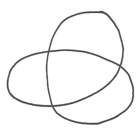
Figure 1.1: A Knot Shadow

Unfortunately, the picture doesn’t show which strand is on top and which strand is below, at each intersection. So the knot in question could be any one of the following eight possibilities.

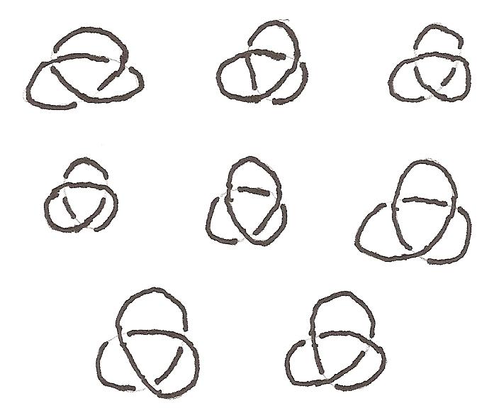
Figure 1.2: Resolutions of Figure 1.1

Ursula and King Lear decide to play a game with Figure 1.1. They take turns alternately resolving a crossing, by choosing which strand is on top. If Ursula goes first, she could move as follows:

King Lear might then respond with

For the third and final move, Ursula might then choose to move to

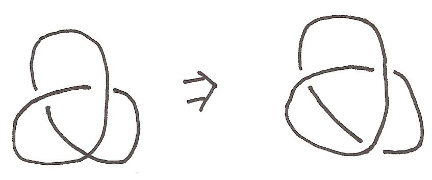
Figure 1.3: The final move

Now the knot is completely identified. In fact, this knot can be untied as follows, so mathematically it is the unknot:

Because the final knot was the unknot, Ursula is the winner - had it been truly knotted, King Lear would be the winner.

A picture of a knot like the ones in Figures 1.2 and 1.3 is called a knot diagram or knot projection in the field of mathematics known as Knot Theory. The generalization in which some crossings are unresolved is called a pseudodiagram - every diagram we have just seen is an example. A pseudodiagram in which all crossing are unresolved is called a knot shadow. While knot diagrams are standard tools of knot theory, pseudodiagrams are a recent innovation by Ryo Hanaki for the sake of mathematically modelling electron microscope images of DNA in which the elevation of the strands is unclear, like the following:

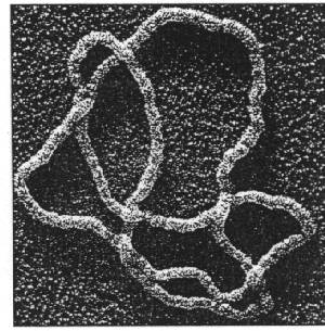
Figure 1.4: Electron Microscope image of DNA

Once upon a time, a group of students in a Research Experience for Undergraduates (REU) at Williams College in 2009 were studying properties of knot pseudodiagrams, specifically the knotting number and trivializing number, which are the smallest number of crossings which one can resolve to ensure that the resulting pseudodiagram corresponds to a knotted knot, or an unknot, respectively. One of the undergraduates had the idea of turning this process into a game between two players, one trying to create an unknot and one trying to create a knot, and thus was born To Knot or Not to Knot (TKONTK), the game described above.

In addition to their paper on knotting and trivialization numbers, the students in the REU wrote an additional Shakespearean-themed paper A Midsummer Knot’s Dream on To Knot or Not to Knot and a couple of other knot games, with names like “Much Ado about Knotting.” In their analysis of TKONTK specifically, they considered starting positions of the following sort:

For these positions, they determined which player wins under perfect play:

• If the number of crossings is odd, then Ursula wins, no matter who goes first.

• If the number of crossings is even, then whoever goes second wins.

They also showed that on a certain large class of shadows, the second player wins.

1.1 Some facts from Knot Theory

In order to analyze TKONTK, or even to play it, we need a way to tell whether a given knot diagram corresponds to the unknot or not. Unfortunately this problem is very non-trivial, and while algorithms exist to answer this question, they are very complicated.

One fundamental fact in knot theory is that two knot diagrams correspond to the same knot if and only if they can be obtained one from the other via a sequence of Reidemeister moves, in addition to mere distortions (isotopies) of the plane in which the knot diagram is drawn. The three types of Reidemeister moves are

1. Adding or removoing a twist in the middle of a straight strand.

2. Moving one strand over another.

3. Moving a strand over a crossing.

These are best explained by a diagram:

Figure 1.5: The three Reidemeister Moves

Given this fact, one way to classify knots is by finding properties of knot diagrams which are invariant under the Reidemeister moves. A number of surprising knot invariants have been found, but none are known to be complete invariants, which exactly determine whether two knots are equivalent.

Although this situation may seem bleak, there are certain families of knots in which we can test for unknottedness easily. One such family is the family of alternating knots. These are knots with the property that if you walk along them, you alternately are on the top or the bottom strand at each successive crossing. Thus the knot weaves under and over itself perfectly. Here are some examples:

The rule for telling whether an alternating knot is the unknot is simple: color the regions between the strands black and white in alternation, and connect the black regions into a graph. Then the knot is the unknot if and only if the graph can be reduced to a tree by removing self-loops. For instance,

is not the unknot, while

is.

Now it turns out that any knot shadow can be turned into an alternating knot - but in only two ways. The players are unlikely to produce one of these two resolutions, so this test for unknottedness is not useful for the game.

Another family of knots, however, works out perfectly for TKONTK. These are the rational knots, defined in terms of the rational tangles. A tangle is like a knot with four loose ends, and two strands. Here are some examples:

The four loose ends should be though of as going off to infinity, since they can’t be pulled in to unknot the tangle. We consider two tangles to be equivalent if you can get from one to the other via Reidemeister moves.

A rational tangle is one built up from the following two

via the following operations:

Now it can easily be seen by induction that if $T$ is a rational tangle, then $T$ is invariant under $180^{\textrm{o}}$ rotations about the $x$, $y$, or $z$ axes:

Because of this, we have the following equivalences,

In other words, adding a twist to the bottom or top of a rational tangle has the same effect, and so does adding a twist on the right or the left. So we can actually build up all rational tangles via the following smaller set of operations:

John Conway found a way to assign a rational number (or $\infty$) to each rational tangle, so that the tangle is determined up to equivalence by its number. Specifically, the initial tangles

have values $0$ and $\infty=1/0$. If a tangle $t$ has value $\frac{p}{q}$, then adding a twist on the left or right changes the value to $\frac{p+q}{q}$ if the twist is left-handed, or $\frac{p-q}{q}$ if the twist is right handed. Adding a twist on the top or bottom changes the value to $\frac{p}{q-p}$ if the twist is left-handed, or $\frac{p}{q+p}$ if the twist is right-handed.

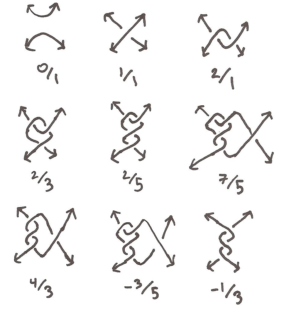
Figure 1.6: Sample rational tangles

Reflecting a tangle over the $45^{\circ}$ diagonal plane corresponds to taking the reciprocal:

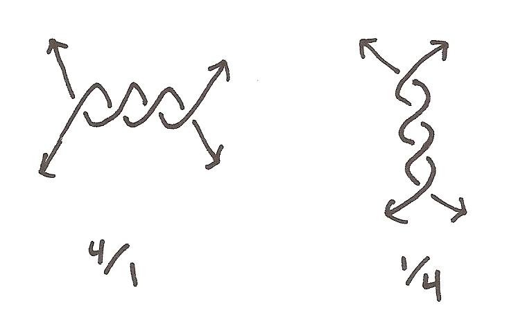
Figure 1.7: Reflection over the diagonal plane corresponds to taking the reciprocal. Note which strands are on top in each diagram.

Using these rules, it’s easy to see that a general rational tangle, built up by adding twists on the bottom or right side, has its value determined by a continued fraction. For instance, the following rational tangle

has value

$$4+\frac{1}{2+\frac{1}{3+\frac{1}{2}}}=\frac{71}{64}.$$

Now a basic fact about continued fractions is that if $n_{1},\ldots,n_{k}$ are positive integers, then the continued fraction

$$n_{1}+\frac{1}{n_{2}+\frac{1}{\ddots+\frac{1}{n_{k}}}}$$

almost encodes the sequence $(n_{1},\ldots,n_{k})$. So this discussion of continued fractions might sound like an elaborate way of saying that rational tangles are determined by the sequence of moves used to construct them.

But our continued fractions can include negative numbers. For instance, the following tangle

has continued fraction

$$3+\frac{1}{-5+\frac{1}{-2+\frac{1}{3}}}=79/28=2+\frac{1}{1+\frac{1}{4+\frac{1}{1+\frac{1}{1+\frac{1}{2}}}}},$$

so that we have the following nontrivial equivalence of tangles:

Given a rational tangle, its numerator closure is obtained by connecting the two strands on top and connecting the two strands on bottom, while the denominator closure is obtained by joining the two strands on the left, and joining the two strands on the right:

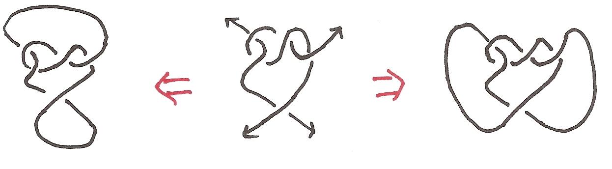
Figure 1.8: the numerator closure (left) and denominator closure (right) of a tangle.

In some cases, the result ends up consisting of two disconnected strands, making it a link rather than a knot:

As a general rule, one can show that the numerator closure is a knot as long as the numerator of $p/q$ is odd, while the denominator closure is a knot as long as the denominator of $p/q$ is odd.

Even better, it turns out that the numerator closure is an unknot exactly if the value $p/q$ is the reciprocal of an integer, and the denominator closure is an unknot exactly if the value $p/q$ is an integer.

The upshot of all this is that if we play TKONTK on a “rational shadow,” like the following:

then at the game’s end the final knot will be rational, and we can check who wins by means of continued fractions.

The twist knots considered in A Midsummer Knot’s Dream are instances of this, since they are the denominator closures of the following rational tangle-shadows:

1.2 Sums of Knots

Now that we have a basic set of analyzable positions to work with, we can quickly extend them by the operation of the connected sum of two knots.

Here are two knots $K_{1}$ and $K_{2}$:

and here is their connected sum $K_{1}\#K_{2}$

This sum may look arbitrary, because it appears to depend on the places where we chose to attach the two knots. However, we can move one knot along the other to change this, as shown in the following picture:

So the place where we choose to join the two knots doesn’t matter.

Our main interest is in the following fact:

Fact 1.2.1.

If $K_{1}$ and $K_{2}$ are knots, then $K_{1}\#K_{2}$ is an unknot if and only if both $K_{1}$ and $K_{2}$ are unknots.

In other words, two non-unknots can never be added and somehow cancel each other. There is actually an interesting theory here, with knots decomposing uniquely as sums of “prime knots.” For more information, and proofs of 1.2.1, I refer the reader to Colin Adams’ The Knot Book.

Because of this fact, we can play To Knot or Not to Knot on sums of rational shadows, like the following

and actually tell which player wins at the end. In fact, the winner will be King Lear as long as he wins in any of the summands, while Ursula needs to win in every summand.

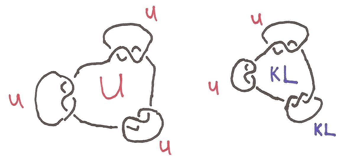
Figure 1.9: On the left, Ursula has won every subgame, so she wins the connected sum. On the right, King Lear has won only one subgame, but this is still enough to make the overall figure knotted, so he wins the connected sum.

Indeed, this holds even when the summands are not rational, though it is harder to tell who wins in that case.

When TKONTK is played on a connected sum of knot shadows, each summand acts as a fully independent game. There is no interaction between the components, except that at the end we pool together the results from each component to see who wins (in an asymmetric way which favors King Lear). We can visualize each component as a black box, whose output gets fed into a logical OR gate to decide the final winner:

The way in which we can add positions of To Knot or Not to Knot together, or decompose positions as sums of multiple non-interacting smaller positions, is highly reminiscent of the branch of recreational mathematics known as combinatorial game theory. Perhaps it can be applied to To Knot or Not to Knot?

The rest of this work is an attempt to do so. We begin with an overview of combinatorial game theory, and then move on to the modifications to the theory that we need to analyze TKONTK. We proceed by an extremely roundabout route, which may perhaps give better insight into the origins of the final theory.

For completeness we include all the basic proofs of combinatorial game theory, though many of them can be found in John Conway’s book On Numbers and Games, and Guy, Berlekamp, and Conway’s book Winning Ways. However ONAG is somewhat spotty in terms of content, not covering Norton multiplication or many of the other interesting results of Winning Ways, while Winning Ways in turn is generally lacking in proofs. Moreover, the proofs of basic combinatorial game theory are the basis for our later proofs of new results, so they are worth understanding.

Part I Combinatorial Game Theory

Chapter 2 Introduction

2.1 Combinatorial Game Theory in general

Combinatorial Game Theory (CGT) is the study of combinatorial games. In the losse sense, these are two-player discrete deterministic games of perfect information:

• There must be only two players. This rules out games like Bridge or Risk.

• The game must be discrete, like Checkers or Bridge, rather than continuous, like Soccer or Fencing.

• There must be no chance involved, ruling out Poker, Risk, and Candyland. Instead, the game must be deterministic.

• At every stage of the game, both players have perfect information on the state of the game. This rules out Stratego and Battleship. Also, there can be no simultaneous decisions, as in Rock-Paper-Scissors. Players must take turns.

• The game must be zero-sum, in the sense of classical game theory. One player wins and the other loses, or the players receive scores that add to zero. This rules out games like Chicken and Prisoner’s Dilemma.

While these criteria rule out most popular games, they include Chess, Checkers, Go, Tic-Tac-Toe, Connect Four, and other abstract strategy games.

By restricting to combinatorial games, CGT distances itself from the classical game theory developed by von Neuman, Morgenstern, Nash, and others. Games studied in classical game theory often model real-world problems like geopolitics, market economics, auctions, criminal justice, and warfare. This makes classical game theory a much more practical and empirical subject that focuses on imperfect information, political coalitions, and various sorts of strategic equilibria. Classical game theory starts begins its analyses by enumerating strategies for all players. In the case of combinatorial games, there are usually too many strategies too list, rendering the techniques of classical game theory somewhat useless.

Given a combinatorial game, we can ask the question: who wins if both players play perfectly? The answer is called the outcome (under perfect play) of the game. The underlying goal of combinatorial game theory is to solve various games by determining their outcomes. Usually we also want a strategy that the winning player can use to ensure victory.

As a simple example, consider the following game: Alice and Bob sit on either side of a pile of beans, and alternately take turns removing 1 or 2 beans from the pile, until the pile is empty. Whoever removes the last bean wins.

If the players start with 37 beans, and Alice goes first, then she can guarantee that she wins by always ending her turn in a configuration where the number of beans remaining is a multiple of three. This is possible on her first turn because she can remove one bean. On subsequent turns, she moves in response to Bob, taking one bean if he took two, and vice versa. So every two turns, the number of beans remaining decreases by three. Alice will make the final move to a pile of zero beans, so she is guaranteed the victory. Because Alice has a perfect winning strategy, Bob has no useful strategies at all, and so all his strategies are “optimal,” because all are equally bad.

On the other hand, if there had been 36 beans originally, and Alice had played first, then Bob would win by the same strategy, taking one or two beans in response to Alice taking two or one beans, respectively. Now Bob will always end his turn with the number of beans being a multiple of three, so he will be the one to move to the position with no beans.

The general solution is as follows:

• If there are $3n+1$ or $3n+2$ beans on the table, then the next player to move will win under perfect play.

• If there are $3n$ beans on the table, then the next player to move will lose under perfect play.

Given this solution, Alice or Bob can consider each potential move, and choose the one which results in the optimal outcome. In this case, the optimal move is to always move to a multiple of three. The players can play perfectly as long as they are able to tell the outcome of an arbitrary position under consideration.

As a general principle, we can say that

In a combinatorial game, knowing the outcome (under perfect play) of every position allows one to play perfectly.

This works because the players can look ahead one move and choose the move with the best outcome. Because of this, the focus of CGT is to determine the outcome (under perfect play) of positions in arbitrary games. Henceforth, we assume that the players are playing perfectly, so that the “outcome” always refers to the outcome under perfect play, and “Ted wins” means that Ted has a strategy guaranteeing a win.

Most games do not admit such simple solutions as the bean-counting game. As an example of the complexities that can arise, consider Wythoff’s Game In this game, there are two piles of beans, and the two players (Alice and Bob) alternately take turns removing beans. In this game, a player can remove any number of beans (more than zero) on her turn, but if she removes beans from both piles, then she must remove the same number from each pile. So if it is Alice’s turn, and the two piles have sizes 2 and 1, she can make the following moves: remove one or two beans from the first pile, remove one bean from the second pile, or remove one bean from each pile. Using $(a,b)$ to represent a state with $a$ beans in one pile and $b$ beans in the other, the legal moves are to states of the form $(a-k,b)$ where $0<k\leq a$, $(a-k,b-k)$, where $0<k\leq\min(a,b)$, and $(a,b-k)$, where $0<k\leq b$. As before, the winner is the player who removes the last bean.

Equivalently, there is a lone Chess queen on a board, and the players take turns moving her south, west, or southwest. The player who moves her into the bottom left corner is the winner. Now $(a,b)$ is the queen’s grid coordinates, with the origin in the bottom left corner.

Wythoff showed that the following positions are the ones you should move to under optimal play - they are the positions for which the next player to move will lose:

$$\left(\lfloor n\phi\rfloor,\lfloor n\phi^{2}\rfloor\right)$$

and

$$\left(\lfloor n\phi^{2}\rfloor,\lfloor n\phi\rfloor\right)$$

where $\phi$ is the golden ratio $\frac{1+\sqrt{5}}{2}$ and $n=0,1,2,\ldots$. (As an aside, the two sequences $a_{n}=\left\lfloor n\phi\right\rfloor$ and $b_{n}=\left\lfloor n\phi^{2}\right\rfloor$:

$$\{a_{n}\}_{n=0}^{\infty}=\{0,1,3,4,6,8,9,\ldots\}$$

$$\{b_{n}\}_{n=0}^{\infty}=\{0,2,5,7,10,13,15,\ldots\}$$

are examples of Beatty sequences, and have several interesting properties. For example, $b_{n}=n+a_{n}$ for every $n$, and each positive integer occurs in exactly one of the two sequences. These facts play a role in the proof of the solution of Wythoff’s game.)

Much of combinatorial game theory consists of results of this sort - independent analyses of isolated games. Consequently, CGT has a tendency to lack overall coherence. The closest thing to a unifying framework within CGT is what I will call Additive Combinatorial Game Theory, by which I mean the theory begun and extended by Sprague, Grundy, Milnor, Guy, Smith, Conway, Berlekamp, Norton, and others. Additive CGT will be the focus of most of this thesis.

2.1.1 Bibliography

The most famous books on CGT are John Conway’s On Numbers and Games, Conway, Guy, and Berlekamp’s four-volume Winning Ways For your Mathematical Plays (referred to as Winning Ways), and three collections of articles published by the Mathematical Sciences Research Institute: Games of No Chance, More Games of No Chance, and Games of No Chance 3. There are also over a thousand articles in other books and journals, many of which are listed in the bibliographies of the Games of No Chance books.

Winning Ways is an encyclopedic work: the first volume covers the core theory of additive CGT, the second covers ways of bending the rules, and the third and fourth volumes apply these theories to various games and puzzles. Conway’s ONAG focuses more closely on the Surreal Numbers (an ordered field extending the real numbers to also include all the transfinite ordinals), for the first half of the book, and then considers additive CGT in the second half. Due to its earlier publication, the second half of ONAG is generally superseded by the first two volumes of Winning Ways, though it tends to give more precise proofs. The Games of No Chance books are anthologies of papers on diverse topics in the field.

Additionally, there are at least two books applying these theories to specific games: Berlekamp’s The Dots and Boxes Game: Sophisticated Child’s Play and Wolfe and Berlekamp’s Mathematical Go: Chilling Gets the Last Point. These books focus on Dots-and-Boxes and Go, respectively.

2.2 Additive CGT specifically

We begin by introducing a handful of example combinatorial games.

The first is Nim, in which there are several piles of counters (as in Figure 2.1), and players take turns alternately removing pieces until none remain. A move consists of removing one or more pieces from a signle pile. The player to remove the last piece wins. There is no set starting position.

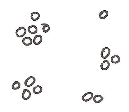
Figure 2.1: A Nim position containing piles of size 6, 1, 3, 2, and 4.

A game of Hackenbush consists of a drawing made of red and blue edges connected to each other, and to the “ground,” a dotted line at the edge of the world. See Figure 2.2 for an example. Roughly, a Hackenbush poition is a graph whose edge have been colored red and blue.

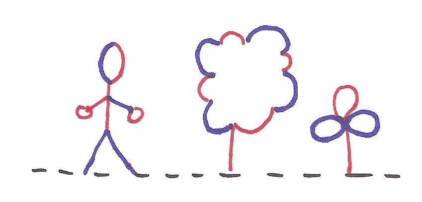
Figure 2.2: A Hackenbush position.

On each turn, the current player chooses one edge of his own color, and erases it. In the process, other edge may become disconnected from the ground. These edges are also erased. If the current player is unable to move, then he loses. Again, there is no set starting position.

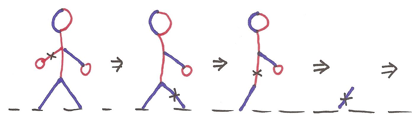
Figure 2.3: Four successive moves in a game of Hackenbush. Red goes first, and Blue makes the final move of this game. Whenever an edge is deleted, all the edges that become disconnected from the ground disappear at the same time.

In Domineering, invented by Göran Andersson, a game begins with an empty chessboard. Two players, named Horizontal and Vertical, place dominoes on the board, as in Figure 2.4. Each domino takes up two directly adjacent squares. Horizontal’s dominoes must be aligned horizontally (East-West), while Vertical’s must be aligned vertically (North-South). Dominoes are not allowed to overlap, so eventually the board fills up. The first player unable to move on his turn loses.

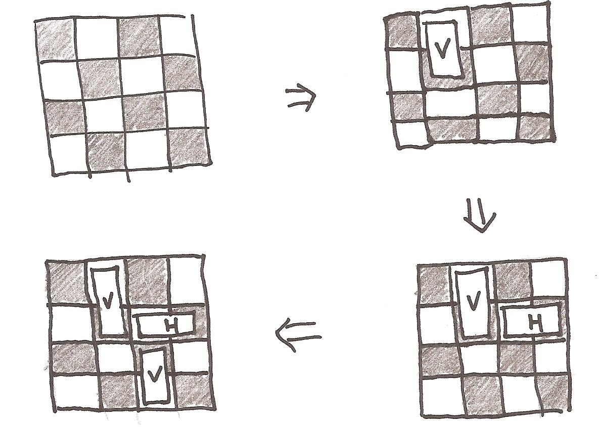
Figure 2.4: Three moves in a game of Domineering. The board starts empty, and Vertical goes first.

A pencil-and-paper variant of this game is played on a square grid of dots. Horizontal draws connects adjacent dots with horizontal lines, and vertical connects adjacent dots with vertical lines. No dot may have more than one line out of it. The reader can easily check that this is equivalent to placing dominoes on a grid of squares.

Clobber is another game played on a square grid, covered with White and Black checkers. Two players, White and Black, alternately move until someone is unable to, and that player loses. A move consists of moving a piece of your own color onto an immediately adjacent piece of your opponent’s color, which gets removed. The game of Konane (actually an ancient Hawaiian gambling game), is played by the same rules, except that a move consists of jumping over an opponent’s piece and removing it, rather than moving onto it, as in Figure 2.5. In both games, the board starts out with the pieces in an alternating checkerboard pattern, except that in Konane two adjacent pieces are removed from the middle, to provide room for the initial jumps.

Figure 2.5: Example moves in Clobber and Konane. In Clobber (top), the capturing piece displaces the captured piece. In Konane (bottom), the capturing piece instead jumps over to the captured piece, to an empty space on the opposite side. Only vertical and horizontal moves are allowed in both games, not diagonal.

The games just described have the following properties in common, in addition to being combinatorial games:

• A player loses when and only when he is unable to move. This is called the normal play convention.

• The games cannot go on forever, and eventually one player wins. In every one of our example games, the number of pieces or parts remaining on the board decreases over time (or in the case of Domineering, the number of empty spaces decreases.) Since all these games are finite, this means that a game can never loop back to a previous position. These games are all loopfree.

• Each game has a tendency to break apart into independent subcomponents. This is less obvious but the motivation for additive CGT. In the Hackenbush position of Figure 2.2, the stick person, the tree, and the flower each functions as a completely independent subgame. In effect, three games of Hackenbush are being played in parallel.

  Similarly, in Domineering, as the board begins to fill up, the remaining empty spaces (which are all that matter from a strategic point of view) will be disconnected into separate clusters, as in Figure 3.1. Each cluster might as well be on a separate board. So again, we find that the two players are essentially playing several games in parallel.

  In Clobber and Konane, as the pieces disappear they begin to fragment into clusters, as in Figure 2.6. In Clobber, once two groups of checkers are disconnected they have no future way of interacting with each other. So in Figure 2.7, each of the red circled regions is an independent subgame. In Konane, pieces can jump into empty space, so it is possible for groups of checkers to reconnect, but once there is sufficient separation, it is often possible to prove that such connection is impossible. Thus Konane splits into independent subgames, like Clobber.

  

  Figure 2.6: Subidivision of Clobber positions: Black’s move breaks up the position into a sum of two smaller positions.

  

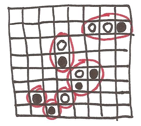
  Figure 2.7: A position of Clobber that decomposes as a sum of independent positions. Each circled area functions independently from the others.

  In Nim, something more subtle happens: each pile is an independent game. As an isolated position, an individual pile is not interesting because whoever goes first takes the whole pile and wins. In combination, however, nontrivial things occur.

  In all these cases, we end up with positions that are sums of other positions. In some sense, additive combinatorial game theory is the study of the nontrivial behavior of sums of game.

The core theory of additive CGT, the theory of partizan games, focuses on loopfree combinatorial games played by the normal play rule. There is no requirement for the games under consideration to decompose as sums, but unless this occurs, the theory has no a priori reason to be useful. Very few real games (Chess, Checkers, Go, Hex) meet these requirements, so Additive CGT has a tendency to focus on obscure games that nobody plays. Of course, this is to be expected, since once a game is solved, it loses its appeal as a playable game.

In many cases, however, a game which does not fit these criteria can be analyzed or partially analyzed by clever applications of the core theory. For example, Dots-and-Boxes and Go have both been studied using techniques from the theory of partizan games. In other cases, the standard rules can be bent, to yield modified or new theories. This is the focus of Part 2 of Winning Ways and Chapter 14 of ONAG, as well as Part II of this thesis.

2.3 Counting moves in Hackenbush

Consider the following Hackenbush position:

Since there are only blue edges present, Red has no available moves, so as soon as his turn comes around, he loses. On the other hand, Blue has at least one move available, so she will win no matter what. To make things more interesting, lets give Red some edges:

Now there are 5 red edges and 8 blue edges. If Red plays wisely, moving on the petals of the flower rather than the stem, he will be able to move 5 times. However Blue can similarly move 8 times, so Red will run out of moves first and lose, no matter which player moves first. So again, Blue is guaranteed a win.

This suggests that we balance the position by giving both players equal numbers of edges:

Now Blue and Red can each move exactly 8 times. If Blue goes first, then she will run out of moves first, and therefore lose, but conversely if Red goes first he will lose. So whoever goes second wins.

In general, if we have a position like

which is a sum of non-interacting red and blue components, then the player with the greater number of edges will win. In the case of a tie, whoever goes second wins. The players are simply seeing how long they can last before running out of moves.

But what happens if red and blue edges are mixed together, like so?

We claim that Blue can win in this position. Once all the blue edges are gone, the red edges must all vanish, because they are disconnected from the ground. So if Red is able to move at any point, there must be blue edges remaining in play, and Blue can move too. Since no move by Red can eliminate blue edges, it follows that after any move by Red, blue edges will remain and Blue cannot possibly lose. This demonstrates that the simple rule of counting edges is no longer valid, since both players have eight edges but Blue has the advantage.

Let’s consider a simpler position:

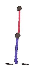
Figure 2.8: How many moves is this worth?

Now Red and Blue each have 1 edge, but for similar reasons to the previous picture, Blue wins. How much of an advantage does Blue have? Let’s add one red edge, giving a 1-move advantage to Red:

Figure 2.9: Figure 2.8 plus a red edge.

Now Red is guaranteed a win! If he moves first, he can move to the following position:

Figure 2.10: A red edge and a blue edge. This position is balanced, so whoever goes next loses. This is a good position to move to.

which causes the next player (Blue) to lose, and if he moves second, he simply ignores the extra red edge on the left and treats Figure 2.9 as Figure 2.10.

So although Figure 2.8 is advantageous for Blue, the advantage is worth less than 1 move. Perhaps Figure 2.8 is worth half a move for Blue? We can check this by adding two copies of Figure 2.8 to a single red edge:

You can easily check that this position is now a balanced second-player win, just like Figure 2.10. So two copies of Figure 2.8 are worth the same as one red edge, and Figure 2.8 is worth half a red edge.

In the same way, we can show for

that (a) is worth $3/4$ of a move for Blue, and (b) is worth $2.5$ moves for Red, because the following two positions turn out to be balanced:

We can combine these values, to see that (a) and (b) together are worth $2.5-3/4=7/4$ moves for Red.

The reader is probably wondering why any of these operations are legitimate. Additive CGT shows that we can assign a rational number to each Hackenbush position, measuring the advantage of that position to Blue. The sign of the number determines the outcome:

• If positive, then Blue will win no matter who goes first.

• If negative, then Red will win no matter who goes first.

• If zero, then whoever goes second will win.

And the number assigned to the sum of two positions is the sum of the numbers assigned to each position. With games other than Hackenbush, we can assign values to positions, but the values will no longer be numbers. Instead they will live in a partially ordered abelian group called Pg. The structure of Pg is somewhat complicated, and is one of the focuses of CGT.

Chapter 3 Games

3.1 Nonstandard Definitions

An obvious way to mathematically model a combinatorial game is as a set of positions with relations to specify how each player can move. This is not the conventional way of defining games in combinatorial game theory, but we will use it at first because it is more intuitive in some ways:

Definition 3.1.1.

A game graph is a set $S$ of positions, a designated starting position $\operatorname{start}(S)\in S$, and two relations $\stackrel{{\scriptstyle L}}{{\to}}$ and $\stackrel{{\scriptstyle R}}{{\to}}$ on $S$. For any $x\in S$, the $y\in S$ such that $x\stackrel{{\scriptstyle L}}{{\to}}y$ are called the left options of $x$, and the $y\in S$ such that $x\stackrel{{\scriptstyle R}}{{\to}}y$ are called the right options of $x$.

For typographical reasons that will become clear in the next section, the two players in additive CGT are almost always named Left and Right. The two relations $\stackrel{{\scriptstyle L}}{{\to}}$ and $\stackrel{{\scriptstyle R}}{{\to}}$ are interpreted as follows: $x\stackrel{{\scriptstyle L}}{{\to}}y$ means that Left can move from position $x$ to position $y$, and $x\stackrel{{\scriptstyle R}}{{\to}}y$ means that Right can move from position $x$ to position $y$. So if the current position is $x$, Left can move to any of the left options of $x$, and Right can move to any of the right options of $x$. We use the shorthand $x\to y$ to denote $x\stackrel{{\scriptstyle L}}{{\to}}y$ or $x\stackrel{{\scriptstyle R}}{{\to}}y$.

The game starts out in the position $s_{0}$. We intentionally do not specify who will move first. There is no need for a game graph to specify which player wins at the game’s end, because we are using the normal play rule: the first player unable to move loses.

But wait - why should the game ever come to an end? We need to add an additional condition: there should be no infinite sequences of play

$$a_{1}\stackrel{{\scriptstyle L}}{{\to}}a_{2}\stackrel{{\scriptstyle R}}{{\to}}a_{3}\stackrel{{\scriptstyle L}}{{\to}}a_{4}\stackrel{{\scriptstyle R}}{{\to}}\cdots.$$

Definition 3.1.2.

A game graph is well-founded or loopfree if there are no infinite sequences of positions $a_{1},a_{2},\ldots$ such that

$$a_{1}\to a_{2}\to a_{3}\to\cdots.$$

We also say that the game graph satisfies the ending condition.

This property might seem like overkill: not only does it rule out

$$a_{1}\stackrel{{\scriptstyle L}}{{\to}}a_{2}\stackrel{{\scriptstyle R}}{{\to}}a_{3}\stackrel{{\scriptstyle L}}{{\to}}a_{4}\stackrel{{\scriptstyle R}}{{\to}}\cdots$$

and

$$a_{1}\stackrel{{\scriptstyle R}}{{\to}}a_{2}\stackrel{{\scriptstyle L}}{{\to}}a_{3}\stackrel{{\scriptstyle R}}{{\to}}a_{4}\stackrel{{\scriptstyle L}}{{\to}}\cdots$$

but also sequences of play in which the players aren’t taking turns correctly, like

$$a_{1}\stackrel{{\scriptstyle R}}{{\to}}a_{2}\stackrel{{\scriptstyle R}}{{\to}}a_{3}\stackrel{{\scriptstyle R}}{{\to}}a_{4}\stackrel{{\scriptstyle L}}{{\to}}a_{5}\stackrel{{\scriptstyle R}}{{\to}}a_{6}\stackrel{{\scriptstyle L}}{{\to}}\cdots.$$

The ending condition is actually necessary, however, when we play sums of games. When games are played in parallel, there is no guarantee that within each component the players will alternate. If Left and Right are playing a game $A+B$, Left might move repeatedly in $A$ while Right moved repeatedly in $B$. Without the full ending condition, the sum of two well-founded games might not be well-founded. If this is not convincing, the reader can take this claim on faith, and also verify that all of the games described above are well-founded in this stronger sense.

The terminology “loopfree” refers to the fact that, when there are only finitely many positions, being loopfree is the same as having no cycles $x_{1}\to x_{2}\to\cdots\to x_{n}\to x_{1}$, because any infinite series would necessarily repeat itself. In the infinite case, the term loopfree might not be strictly accurate.

A key fact of well-foundedness, which will be fundamental in everything that follows, is that it gives us an induction principle

Theorem 3.1.3.

Let $S$ be the set of positions in a well-founded game graph, and let $P$ some subset of $S$. Suppose that $P$ has the following property: if $x\in S$ and every left and right option of $x$ is in $P$, then $x\in P$. Then $P=S$.

Proof.

Let $P^{\prime}=S\setminus P$. Then by assumption, for every $x\in P^{\prime}$, there is some $y\in P^{\prime}$ such that $x\to y$. Suppose for the sake of contradiction that $P^{\prime}$ is nonempty. Take $x_{1}\in P^{\prime}$, and find $x_{2}\in P^{\prime}$ such that $x_{1}\to x_{2}.$ Then find $x_{3}\in P^{\prime}$ such that $x_{2}\to x_{3}$. Repeating this indefinitely we get an infinite sequence

$$x_{1}\to x_{2}\to\cdots$$

contradicting the assumption that our game graph is well-founded. ∎

To see the similarity with induction, suppose that the set of positions is $\{1,2,\ldots,n\}$, and $x\to y$ iff $x>y$. Then this is nothing but strong induction.

As a first application of this result, we show that in a well-founded game graph, somebody has a winning strategy. More precisely, every position in a well-founded game graph can be put into one of four outcome classes:

• Positions that are wins for Left, no matter which player moves next.

• Positions that are wins for Right, no matter which player moves next.

• Positions that are wins for whichever player moves next.

• Positions that are wins for whichever player doesn’t move next (the previous player).

These four possible outcomes are abbreviated as $L$, $R$, $1$ and $2$.

Theorem 3.1.4.

Let $S$ be the set of positions of a well-founded game graph. Then every position in $S$ falls into one of the four outcome classes.

Proof.

Let $L_{1}$ be the set of positions that are wins for Left when she goes first, $R_{1}$ be the set of positions that are wins for Right when he goes first, $L_{2}$ be the set of positions that are wins for Left when she goes second, and $R_{2}$ be the set of positions that are wins for Right when he goes second.

The reader can easily verify that a position $x$ is in

• $L_{1}$ iff some left option is in $L_{2}$.

• $R_{1}$ iff some right option is in $R_{2}$.

• $L_{2}$ iff every right option is in $L_{1}$.

• $R_{2}$ iff every left option is in $R_{1}$.

These rules are slightly subtle, since they implicitly contain the normal play convention, in the case where $x$ has no options.

If Left goes first from a given position $x$, we want to show that either Left or Right has a winning strategy, or in other words that $x\in L_{1}$ or $x\in R_{2}$. Similarly, we want to show that every position is in either $R_{1}$ or $L_{2}$. Let $P$ be the set of positions for which $x$ is in exactly one of $L_{1}$ and $R_{2}$ and in exactly one of $R_{1}$ and $L_{2}$. By the induction principle, it suffices to show that when all options of $x$ are in $P$, then $x$ is in $P$. So suppose all options of $x$ are in $P$. Then the following are equivalent:

• $x\in L_{1}$

• some option of $x$ is in $L_{2}$

• some option of $x$ is not in $R_{1}$

• not every option of $x$ is in $R_{1}$

• $x$ is not in $R_{2}$.

Here the equivalence of the second and third line follows from the inductive hypothesis, and the rest follows from the reader’s exercise. So $x$ is in exactly one of $L_{1}$ and $R_{2}$. A similar argument shows that $x$ is in exactly one of $R_{1}$ and $L_{2}$. So by induction every position is in $P$.

So every position is in one of $L_{1}$ and $R_{2}$, and one of $R_{1}$ and $L_{2}$. This yields four possibilities, which are the four outcome classes:

• $L_{1}\cap R_{1}=1$.

• $L_{1}\cap L_{2}=L$.

• $R_{2}\cap R_{1}=R$.

• $R_{2}\cap L_{2}=2$.

∎

Definition 3.1.5.

The outcome of a game is the outcome class (1, 2, L, or R) of its starting position.

Now that we have a theoretical handle on perfect play, we turn towards sums of games.

Definition 3.1.6.

If $S_{1}$ and $S_{2}$ are game graphs, we define the sum $S_{1}+S_{2}$ to be a game graph with positions $S_{1}\times S_{2}$ and starting position $\operatorname{start}(S_{1}+S_{2})=(\operatorname{start}(S_{1}),\operatorname{start}(S_{2}))$. The new $\stackrel{{\scriptstyle L}}{{\to}}$ relation is defined by

$$(x,y)\stackrel{{\scriptstyle L}}{{\to}}(x^{\prime},y^{\prime})$$

if $x=x^{\prime}$ and $y\stackrel{{\scriptstyle L}}{{\to}}y^{\prime}$, or $x\stackrel{{\scriptstyle L}}{{\to}}x^{\prime}$ and $y=y^{\prime}$. The new $\stackrel{{\scriptstyle R}}{{\to}}$ is defined similarly.

This definition generalizes in an obvious way to sums of three or more games. This operation is essentially associative and commutative, and has as its identity the zero game, in which there is a single position from which neither player can move.

In all of our example games, the sum of two positions can easily be constructed. In Nim, we simply place the two positions side by side. In fact this is literally what we do in each of the games in question. In Clobber, one needs to make sure that the two positions aren’t touching, and in Konane, the two positions need to be kept a sufficient distance apart. In Domineering, the focus is on the empty squares, so one needs to “add” the gaps together, again making sure to keep them separated. And as noted above, such composite sums occur naturally in the course of each of these games.

Figure 3.1: The Domineering position on the left decomposes as a sum of the two positions on the right.

Another major operation that can be performed on games: is negation:

Definition 3.1.7.

If $S$ is a game graph, the negation $-S$ has the same set of positions, and the same starting position, but $\stackrel{{\scriptstyle L}}{{\to}}$ and $\stackrel{{\scriptstyle R}}{{\to}}$ are interchanged.

Living up to its name, this operation will turn out to actually produce additive inverses, modulo Section 3.3. This operation is easily exhibited in our example games (see Figure 3.2 for examples):

• In Hackenbush, negation reverses the color of all the red and blue edges.

• In Domineering, negation corresponds to reflecting the board over a 45 degree line.

• In Clobber and Konane, it corresponds to changing the color of every piece.

• Negation has no effect on Nim-positions. This works because $\stackrel{{\scriptstyle L}}{{\to}}$ and $\stackrel{{\scriptstyle R}}{{\to}}$ are the same in any position of Nim.

So in general, negation interchanges the roles of the two players.

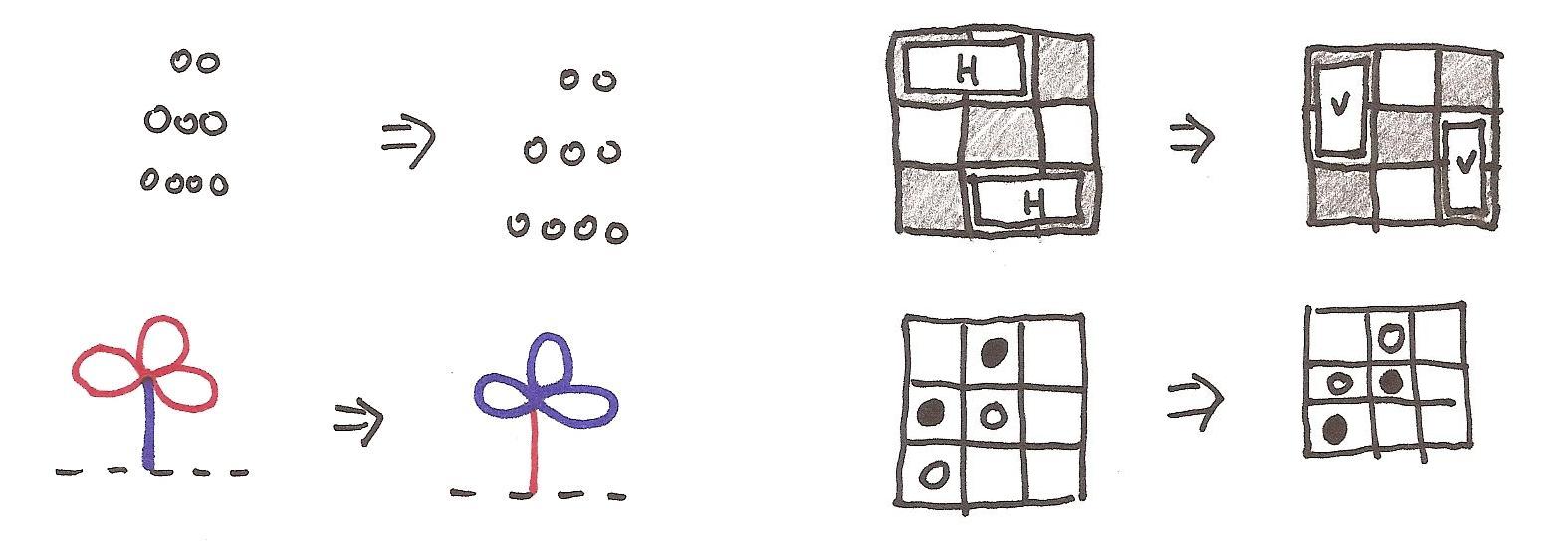
Figure 3.2: Negation in its various guises.

We also define subtraction of games by letting

$$G-H=G+(-H).$$

3.2 The conventional formalism

While there are no glaring problems with “game graphs,” a different convention is used in literature. We merely included it here because it is slightly more intuitive than the actual definition we are going to give later in this section. And even this defintion will be lacking one last clarification, namely Section 3.3.

To motivate the standard formalism, we turn to an analogous situation in set theory: well-ordered sets.

A well-ordered set is a set $S$ with a relation $>$ having the following properties:

• Irreflexitivity: $a>a$ is never true.

• Transitivity: if $a>b$ and $b>c$ then $a>c$.

• Totality: for every $a,b\in S$, either $a>b$, $a=b$, or $a<b$.

• Well-orderedness: there are no infinite descending chains

  $$x_{1}>x_{2}>x_{3}>\cdots$$

These structures are very rigid, and there is a certain canonical list of well-ordered sets called the von Neumann ordinals. A von Neumann ordinal is rather opaquely defined as a set $S$ with the property that $S$ and all its members are transitive. Here we say that a set is transitive if it contains all members of its members.

Given a von Neumann ordinal $S$, we can define a well-ordering on $S$ be letting $x>y$ mean $y\in x$. Moreover each well-ordered set is isomorphic to a unique von Neuman ordinal. The von Neumann ordinals themselves are well-ordered by $\in$, and the first few are

$$0=\{\}=\emptyset$$

$$1=\{\{\}\}=\{0\}$$

$$2=\{\{\},\{\{\}\}\}=\{0,1\}$$

$$3=\{\{\},\{\{\}\},\{\{\},\{\{\}\}\}\}=\{0,1,2\}$$

$$\vdots$$

In general, each von Neumann ordinal is the set of preceding ordinals - for instance, the first infinite ordinal number is $\omega=\{0,1,2,\ldots\}$.

In some sense, the point of (von Neumann) ordinal numbers is to provide canonical instances of each isomorphism class of well-ordered sets. Well-ordered sets are rarely considered in their own right, because the theory immediately reduces to the theory of ordinal numbers. Something similar will happen with games - each isomorphism class of game graphs will be represented by a single game. This will be made possible through the magic of well-foundedness.

Analogous to our operations on game graphs, there are certain ways one can combine well-ordered sets. For instance, if $S$ and $T$ are well-ordered sets, then one can produce (two!) well-orderings of the disjoint union $S\coprod T$, by putting all the elements of $S$ before (or after) $T$. And similarly, we can give $S\times T$ a lexicographical ordering, letting $(s_{1},t_{1})<(s_{2},t_{2})$ if $t_{1}<t_{2}$ or ($s_{1}<s_{2}$ and $t_{1}=t_{2}$). This also turns out to be a well-ordering.

These operations give rise to the following recursively-defined operations on ordinal numbers, which don’t appear entirely related:

• $\alpha+\beta$ is defined to be $\alpha$ if $\beta=0$, the successor of $\alpha+\beta^{\prime}$ if $\beta$ is the successor of $\beta^{\prime}$, and the supremum of $\{\alpha+\beta^{\prime}\,:\,\beta^{\prime}<\beta\}$ if $\beta$ is a limit ordinal.

• $\alpha\beta$ is defined to be $0$ if $\beta=0$, defined to be $\alpha\beta^{\prime}+\alpha$ if $\beta$ is the successor of $\beta^{\prime}$, and defined to be the supremum of $\{\alpha\beta^{\prime}\,:\,\beta^{\prime}<\beta\}$ if $\beta$ is a limit ordinal.

In what follows, we will give recursive definitions of “games,” and also of their outcomes, sums, and negatives. These definitions might seem strange, so we invite the reader to check that they actually come out to the right things, and agree with the definitions given in the last section.

The following definition is apparently due to John Conway:

Definition 3.2.1.

A (partizan) game is an ordered pair $(L,R)$ where $L$ and $R$ are sets of games. If $L=\{A,B,\ldots\}$ and $R=\{C,D,\ldots\}$, then we write $(L,R)$ as

$$\{A,B,\ldots|C,D,\ldots\}.$$

The elements of $L$ are called the left options of this game, and the elements of $R$ are called its right options. The positions of a game $G$ are $G$ and all the positions of the options of $G$.

Following standard conventions in the literature, we will always denote direct equality between partizan games with $\equiv$, and refer to this relation as identity.

Not only does the definition of “game” appear unrelated to combinatorial games, it also seems to be missing a recursive base case.

The trick is to begin with the empty set, which gives us the following game

$$0\equiv(\emptyset,\emptyset)\equiv\{|\}.$$

Once we have one game, we can make three more:

$$1\equiv\{0|\}$$

$$-1\equiv\{|0\}$$

$$*\equiv\{0|0\}$$

The reason for the numerical names like $0$ and $1$ will become clear later.

In order to avoid a proliferation of brackets, we use $||$ to indicate a higher level of nesting:

$$\{w,x||y|z\}\equiv\{w,x|\{y|z\}\}$$

$$\{a|b||c|d\}\equiv\{\{a|b\}|\{c|d\}\}$$

The interpretation of $(L,R)$ is a position whose left options are the elements of $L$ and right options are the elements of $R$. In particular, this shows us how to associate game graphs with games:

Theorem 3.2.2.

Let $S$ be a well-founded game graph. Then there is a unique function $f$ assigning a game to each position of $S$ such that for every $x\in S$, $f(x)\equiv(L,R)$, where

$$L=\{f(y):x\stackrel{{\scriptstyle L}}{{\to}}y\}$$

$$R=\{f(y):x\stackrel{{\scriptstyle R}}{{\to}}y\}$$

In other words, for every position $x$, the left and right options of $f(x)$ are the images of the left and right options of $x$ under $f$.

Moreover, if we take a partizan game $G$, we can make a game graph $S$ by letting $S$ be the set of all positions of $G$, $\operatorname{start}(S)=G$, and letting

$$(L,R)\stackrel{{\scriptstyle L}}{{\to}}x\iff x\in L$$

$$(L,R)\stackrel{{\scriptstyle R}}{{\to}}x\iff x\in R$$

Then the map $f$ sends each element of $S$ to itself.

This theorem is a bit like the Mostowski collapse lemma of set theory, and the proof is similar. Since we will make no formal use of game graphs, we omit the proof, which mainly consists of set theoretic technicalities.

As an example, for Hackenbush positions we have

where

where

and so on. Also see Figure 3.3 for examples of $0$, $1$, $-1$, and $*$ in their various guises in our sample games.

The terms “game” and “position” are used interchangeably in the literature, identifying a game with its starting position. This plays into the philosophy of evaluating every position and assuming the players are smart enough to look ahead one move. Then we can focus on outcomes rather than strategies.

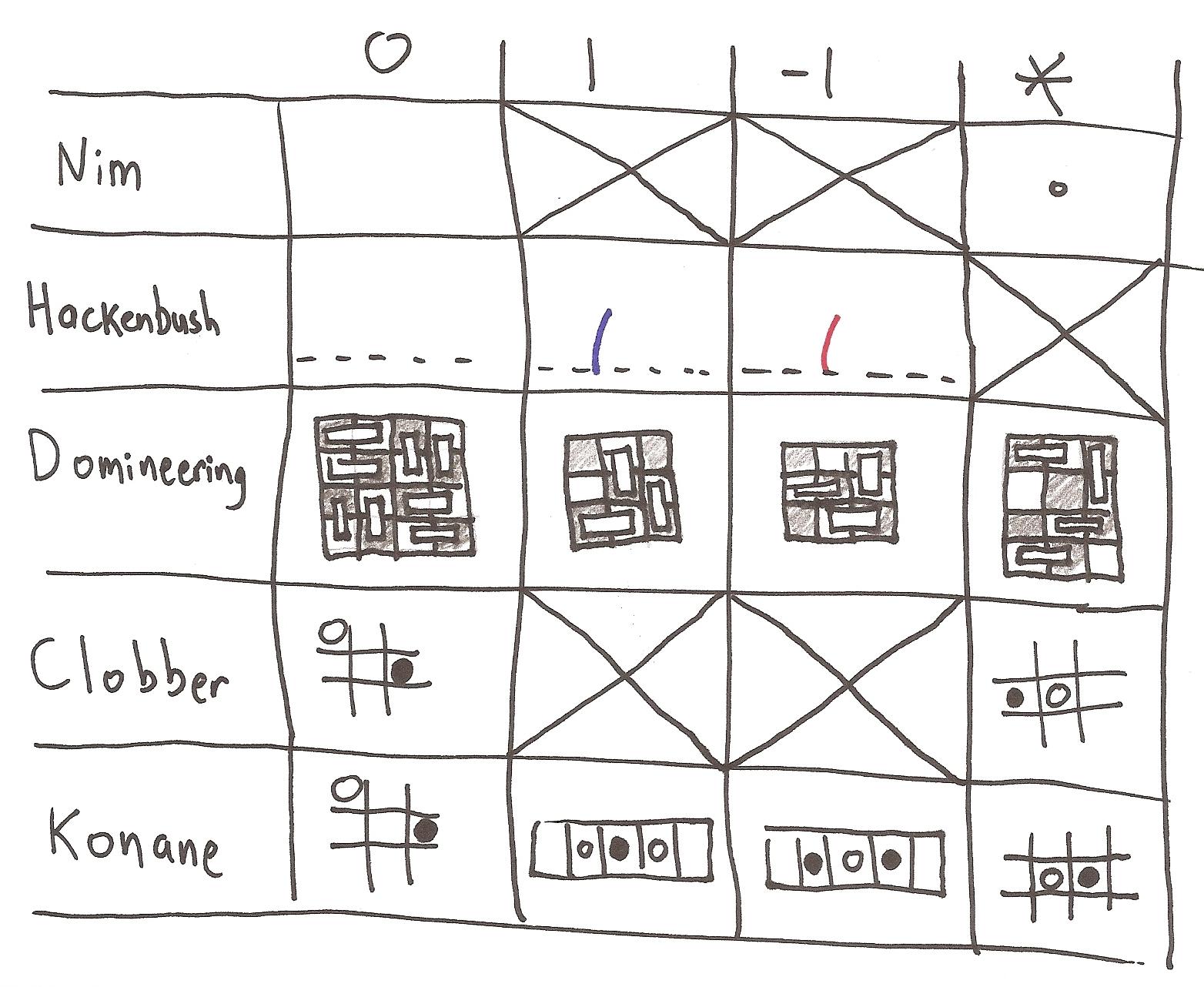
Figure 3.3: The games $0$, $1$, $-1$, and $*$ in their various guises in our sample games. Some cases do not occur - for instance $*$ cannot occur in Hackenbush, and $1$ cannot occur in Clobber. We will see why in Sections 4.3 and 5.1.

Another way to view what’s going on is to consider $\{\cdot|\cdot\}$ as an extra operator for combining games, one that construct a new game with specified left options and specified right options.

We next define the “outcome” of a game, but change notation, to match the standard conventions in the field:

• $G\geq 0$ means that Left wins when Right goes first.

• $G\lhd 0$ means that Right wins when Right goes first.

• $G\leq 0$ means that Right wins when Left goes first.

• $G\rhd 0$ means that Left wins when Right goes first.

The $\rhd$ and $\lhd$ are read as “greater than or fuzzy with” and “less than or fuzzy with.”

These are defined recursively and opaquely as:

Definition 3.2.3.

If $G$ is a game, then

• $G\geq 0$ iff every right option $G^{R}$ satisfies $G^{L}\rhd 0$.

• $G\leq 0$ iff every left option $G^{L}$ satisfies $G^{R}\lhd 0$.

• $G\rhd 0$ iff some left option $G^{L}$ satisfies $G^{L}\geq 0$.

• $G\lhd 0$ iff some right option $G^{R}$ satisfies $G^{R}\leq 0$.

One can easily check that exactly one of $G\geq 0$ and $G\lhd 0$ is true, and exactly one of $G\leq 0$ and $G\rhd 0$ is true.

We then define the four outcome classes as follows:

• $G>0$ iff Left wins no matter who goes first, i.e., $G\geq 0$ and $G\rhd 0$.

• $G<0$ iff Right wins no matter who goes first, i.e., $G\leq 0$ and $G\lhd 0$.

• $G=0$ iff the second player wins, i.e., $G\leq 0$ and $G\geq 0$.

• $G||0$ (read $G$ is incomparable or fuzzy with zero) iff the first player wins, i.e., $G\rhd 0$ and $G\lhd 0$.

Here is a diagram summarizing the four cases:

The use of relational symbols like $>$ and $<$ will be justified in the next section.

If you’re motivated, you can check that these definitions agree with our definitions for well-founded game graphs.

As an example, the four games we have defined so far fall into the four classes:

$$0=0$$

$$1>0$$

$$-1<0$$

$$*||0$$

Next, we define negation:

Definition 3.2.4.

If $G\equiv\{A,B,\ldots|C,D,\ldots\}$ is a game, then its negation $-G$ is recursively defined as

$$-G\equiv\{-C,-D,\ldots|-A,-B,\ldots\}$$

Again, this agrees with the definition for game graphs. As an example, we note the negations of the games defined so far

$$-0\equiv 0$$

$$-1\equiv-1$$

$$-(-1)\equiv 1$$

$$-*\equiv*$$

In particular, the notation $-1$ remains legitimate.

Next, we define addition:

Definition 3.2.5.

If $G\equiv\{A,B,\ldots|C,D,\ldots\}$ and $H\equiv\{E,F,\ldots|X,Y,\ldots\}$ are games, then the sum $G+H$ is recursively defined as

$$G+H=\{G+E,G+F,\ldots,A+H,B+H,\ldots|$$

$$G+X,G+Y,\ldots,H+C,H+D,\ldots\}$$

This definition agrees with our definition for game graphs, though it may not be very obvious. As before, we define subtraction by

$$G-H=G+(-H).$$

The usual shorthand for these definitions is

$$-G\equiv\{-G^{R}|-G^{L}\}$$

$$G+H\equiv\{G^{L}+H,G+H^{L}|G^{R}+H,G+H^{R}\}$$

$$G-H\equiv\{G^{L}-H,G-H^{R}|G^{R}-H,G-H^{L}\}$$

Here $G^{L}$ and $G^{R}$ stand for “generic” left and right options of $G$, and represent variables ranging over all left and right options of $G$. We will make use of this compact and useful notation, which seems to be due to Conway, Guy, and Berlekamp.

We close this section with a list of basic identities satisfied by the operations defined so far:

Lemma 3.2.6.

If $G$, $H$, and $K$ are games, then

$$G+H\equiv H+G$$

$$(G+H)+K\equiv G+(H+K)$$

$$-(-G)\equiv G$$

$$G+0\equiv G$$

$$-(G+H)\equiv(-G)+(-H)$$

$$-0\equiv 0$$

Proof.

All of these are intuitively obvious if you interpret them within the context of Hackenbush, Domineering, or more abstractly game graphs. But the rigorous proofs work by induction. For instance, to prove $G+H\equiv H+G$, we proceed by joint induction on $G$ and $H$. Then we have

$$G+H\equiv\{G^{L}+H,G+H^{L}|G^{R}+H,G+H^{R}\}$$

$$\equiv\{H+G^{L},H^{L}+G|H+G^{R},H^{R}+G\}\equiv H+G,$$

where the outer identities follow by definition, and the inner one follows by the inductive hypothesis. These inductive proofs need no base case, because the recursive definition of “game” had no base case. ∎

On the other hand, $G-G\not\equiv 0$ for almost all games $G$. For instance, we have

$$1-1\equiv 1+(-1)\equiv\{1^{L}+(-1),1+(-1)^{L}|1^{R}+(-1),1+(-1)^{R}\}$$

$$\equiv\{0+(-1)|1+0\}\equiv\{-1|1\}$$

Here there are no $1^{R}$ or $(-1)^{L}$, since $1$ has no right options and $-1$ has no left options.

Definition 3.2.7.

A short game is a partizan game with finitely many positions.

We will assume henceforth that all our games are short. Many of the results hold for general partizan games, but a handful do not, and we have no interest in infinite games.

3.3 Relations on Games

So far, we have done nothing but give complicated definitions of simple concepts. In this section, we begin to look at how our operations for combining games interact with their outcomes.

Above, we defined $G\geq 0$ to mean that $G$ is a win for Left, when Right moves first. Similarly, $G\rhd 0$ means that $G$ is a win for Left when Left moves first. From Left’s point of view, the positions $\geq 0$ are the good positions to move to, and the positions $\rhd 0$ are the ones that Left would like to receive from her opponent. In terms of options,

• $G$ is $\geq 0$ iff every one of its right option $G^{R}$ is $\rhd 0$

• $G$ is $\rhd 0$ iff at least one of its left option $G^{L}$ is $\geq 0$.

One basic fact about outcomes of sums is that if $G\geq 0$ and $H\geq 0$, then $G+H\geq 0$. That is, if Left can win both $G$ and $H$ as the second player, then she can also win $G+H$ as the second player. She proceeds by combining her strategy in each summand. Whenever Right moves in $G$ she replies in $G$, and whenever Right moves in $H$ she replies in $H$. Such responses are always possible because of the assumption that $G\geq 0$ and $H\geq 0$.

Similarly, if $G\rhd 0$ and $H\geq 0$, then $G+H\rhd 0$. Here left plays first in $G$, moving to a position $G^{L}\geq 0$, and then notes that $G^{L}+H\geq 0$.

Properly speaking, we prove both statements together by induction:

• If $G,H\geq 0$, then every right option of $G+H$ is of the form $G^{R}+H$ or $G+H^{R}$ by definition. Since $G$ and $H$ are $\geq 0$, $G^{R}$ or $H^{R}$ will be $\rhd 0$, and so every right option of $G+H$ is the sum of a game $\geq 0$ and a game $\rhd 0$. By induction, such a sum will be $\rhd 0$. So every right option of $G+H$ is $\rhd 0$, and therefore $G+H\geq 0$.

• If $G\rhd 0$ and $H\geq 0$, then $G$ has a left option $G^{L}\geq 0$. Then $G^{L}+H$ is the sum of two games $\geq 0$. So by induction $G^{L}+H\geq 0$. But it is a left option of $G+H$, so $G+H\rhd 0$.

Now one can easily see that

$$G\leq 0\iff-G\geq 0$$ (3.1)

and

$$G\lhd 0\iff G\rhd 0.$$ (3.2)

Using these, it similarly follows that if $G\leq 0$ and $H\leq 0$, then $G+H\leq 0$, among other things.

Another result about outcomes is that $G+(-G)\geq 0$. This is shown using what Winning Ways calls the Tweedledum and Tweedledee Strategy.

Here we see the sum of a Hackenbush position and its negative. If Right moves first, then Left can win as follows: whenever Right moves in the first summand, Left makes the corresponding move in the second summand, and vice versa. So if Right initially moves to $G^{R}+(-G)$, then Left moves to $G^{R}+(-(G^{R}))$, which is possible because $-(G^{R})$ is a left option of $-G$. On the other hand, if Right initially moves to $G+(-(G^{L}))$, then Left responds by moving to $G^{L}+(-(G^{L}))$. Either way, Left can always move to a position of the form $H+(-H)$, for some position $H$ of $G$.

More precisely, we prove the following facts

• $G+(-G)\geq 0$

• $G^{R}+(-G)\rhd 0$ if $G^{R}$ is a right option of $G$.

• $G+(-(G^{L}))\rhd 0$ if $G^{L}$ is a left option of $G$.

together jointly by induction:

• For any game $G$, every Right option of $G+(-G)$ is of the form $G^{R}+(-G)$ or $G+(-(G^{L}))$, where $G^{R}$ ranges over right options of $G$ and $G^{L}$ ranges over left options of $G$. This follows from the definitions of addition and negation. By induction all of these options are $\rhd 0$, and so $G+(-G)\geq 0$.

• If $G^{R}$ is a right option of $G$, then $-(G^{R})$ is a left option of $-G$, so $G^{R}+(-(G^{R}))$ is a left option of $G^{R}+(-G)$. By induction $G^{R}+(-(G^{R}))\geq 0$, so $G^{R}+(-G)\rhd 0$.

• If $G^{L}$ is a left option of $G$, then $G^{L}+(-(G^{L}))$ is a left option of $G+(-(G^{L}))$, and by induction $G^{L}+(-(G^{L}))\geq 0$. So $G+(-(G^{L}))\rhd 0$.

We summarize our results in the following lemma.

Lemma 3.3.1.

Let $G$ and $H$ be games.

(a)

If $G\geq 0$ and $H\geq 0$, then $G+H\geq 0$.

(b)

If $G\rhd 0$ and $H\geq 0$, then $G+H\rhd 0$.

(c)

If $G\leq 0$ and $H\leq 0$, then $G+H\leq 0$.

(d)

If $G\lhd 0$ and $H\leq 0$, then $G+H\lhd 0$.

(e)

$G+(-G)\leq 0$ and $G+(-G)\geq 0$, i.e., $G+(-G)=0$.

(f)

If $G^{L}$ is a left option of $G$, then $G^{L}+(-G)\lhd 0$.

(g)

If $G^{R}$ is a right option of $G$, then $G^{R}+(-G)\rhd 0$.

These results allow us to say something about zero games (not to be confused with the zero game $0$).

Definition 3.3.2.

A game $G$ is a zero game if $G=0$.

Namely, zero games have no effect on outcomes:

Corollary 3.3.3.

If $H=0$, then $G+H$ has the same outcome as $G$ for every game $H$.

Proof.

Since $H\geq 0$ and $H\leq 0$, we have by part (a) of Lemma 3.3.1

$$G\geq 0\Rightarrow G+H\geq 0.$$

By part (b)

$$G\rhd 0\Rightarrow G+H\rhd 0.$$

By part (c)

$$G\leq 0\Rightarrow G+H\leq 0.$$

By part (d)

$$G\lhd 0\Rightarrow G+H\lhd 0.$$

So in every case, $G+H$ has whatever outcome $G$ has. ∎

This in some sense justifies the use of the terminology $H=0$, since this implies that $G+H$ and $G+0\equiv G$ always have the same outcome.

We can generalize this sort of equivalence:

Definition 3.3.4.

If $G$ and $H$ are games, we write $G=H$ (read $G$ equals $H$) to mean $G-H=0$. Similarly, if $\Box$ is any of $||$ $<$, $>$, $\geq$, $\leq$, $\lhd$, or $\rhd$, then we use $G\Box H$ to denote $G-H\Box 0$.

Note that since $G+(-0)\equiv G$, this notation does not conflict with our notation for outcomes. The interpretation of $\geq$ is that $G\geq H$ if $G$ is at least as good as $H$, from Left’s point of view, or that $H$ is better than $G$, from Right’s point of view. Similarly, $G=H$ should mean that $G$ and $H$ are strategically equivalent. Further results will justify these intuitions.

These relations have the properties that one would hope for. It’s clear that $G=H$ iff $G\leq H$ and $G\geq H$, or that $G\geq H$ iff $G>H$ or $G=H$. Also, $G\rhd H$ iff $G\not\leq H$. Somewhat less obviously,

$$G\leq H\iff G+(-H)\leq 0\iff-(G+(-H))\equiv H+(-G)\geq 0\iff H\geq G$$

and

$$G\lhd H\iff G+(-H)\lhd 0\iff-(G+(-H))\equiv H+(-G)\rhd 0\iff H\rhd G$$

using equations (3.1-3.2). So we see that $G=H$ iff $H=G$, i.e., $=$ is symmetric.

Moreover, part (e) of Lemma 3.3.1 shows that $G=G$, so that = is reflexive. In fact,

Lemma 3.3.5.

The relations $=$, $\geq$, $\leq$, $>$, and $<$ are transitive. And if $G\leq H$ and $H\lhd K$, then $G\lhd K$. Similarly if $G\lhd H$ and $H\leq K$, then $G\lhd K$.

Proof.

We first show that $\geq$ is transitive. If $G\geq H$ and $H\geq K$, then by definition $G+(-H)\geq 0$ and $H+(-K)\geq 0$. By part (a) of Lemma 3.3.1,

$$(G+(-K))+(H+(-H))\equiv(G+(-H))+(H+(-K))\geq 0.$$

But by part (e), $H+(-H)$ is a zero game, so we can (by the Corollary), remove it without effecting the outcome. Therefore $G+(-K)\geq 0$, i.e., $G\geq K$. So $\geq$ is transitive. Therefore so are $\leq$ and $=$.

Now if $G\leq H$ and $H\lhd K$, suppose for the sake of contradiction that $G\lhd K$ is false. Then $K\leq G\leq H$, so $K\leq H$, contradicting $H\lhd K$. A similar argument shows that if $G\lhd H$ and $H\leq K$, then $G\lhd K$.

Finally, suppose that $G<H$ and $H<K$. Then $G\leq H$ and $H\leq K$, so $G\leq K$. But also, $G\lhd H$ and $H\leq K$, so $G\lhd K$. Together these imply that $G<K$. A similar argument shows that $>$ is transitive. ∎

So we have just shown that $\geq$ is a preorder (a reflexive and transitive relation), with $=$ as its associated equivalence relation (i.e., $x=y$ iff $x\geq y$ and $y\geq x$). So $\geq$ induces a partial order on the quotient of games modulo $=$. Because the outcome depends only on a game’s comparison to 0, it follows that if $G=H$ then $G$ and $H$ have the same outcome.

We use $\mathbf{Pg}$ to denote the class of all partizan games, modulo $=$. This class is also sometimes denoted with Ug (for unimpartial games) in older books. We will use $\mathcal{G}$ to denote the class of all short games modulo $=$. The only article I have seen which explicitly names the group of short games is David Moews’ article The Abstract Structure of the Group of Games in More Games of No Chance, which uses the notation ShUg. This notation is outdated, however, as it is based on the older Ug rather than Pg. Both ShUg and ShPg are notationally ugly, and scattered notation in several other articles suggests we use $\mathcal{G}$ instead.

From now on, we use “game” to refer to an element of $\mathbf{Pg}$.

When we need to speak of our old notion of game, we talk of the “form” of a game, as opposed to its “value,” which is the corresponding representative in Pg. We abuse notation and use $\{A,B,\ldots|C,D,\ldots\}$ to refer to both the form and the corresponding value.

But after making these identifications, can we still use our operations on games, like sums and negation? An analogous question arises in the construction of the rationals from the integers. Usually one defines a rational number to be a pair $\frac{x}{y}$, where $x,y\in\mathbb{Z}$, $y\neq 0$. But we identify $\frac{x}{y}=\frac{x^{\prime}}{y^{\prime}}$ if $xy^{\prime}=x^{\prime}y$. Now, given a definition like

$$\frac{x}{y}+\frac{a}{b}=\frac{xb+ay}{yb},$$

we have to verify that the right hand side does not depend on the form we choose to represent the summands on the left hand side. Specifically, we need to show that if $\frac{x}{y}=\frac{x^{\prime}}{y^{\prime}}$ and $\frac{a}{b}=\frac{a^{\prime}}{b^{\prime}}$, then

$$\frac{xb+ay}{yb}=\frac{x^{\prime}b^{\prime}+a^{\prime}y^{\prime}}{y^{\prime}b^{\prime}}.$$

This indeed holds, because

$$(xb+ay)(y^{\prime}b^{\prime})=(xy^{\prime})(bb^{\prime})+(ab^{\prime})(yy^{\prime})=(x^{\prime}y)(bb^{\prime})+(a^{\prime}b)(yy^{\prime})=(x^{\prime}b^{\prime}+a^{\prime}y^{\prime})(yb).$$

Similarly, we need to show for games that if $G=G^{\prime}$ and $H=H^{\prime}$, then $G+H=G^{\prime}+H^{\prime}$. In fact, we have

Theorem 3.3.6.

(a)

If $G\geq G^{\prime}$ and $H\geq H^{\prime}$, then $G+H\geq G^{\prime}+H^{\prime}$. In particular if $G=G^{\prime}$ and $H=H^{\prime}$, then $G+H=G^{\prime}+H^{\prime}$.

(b)

If $G\geq G^{\prime}$, then $-G^{\prime}\geq-G$. In particular if $G=G^{\prime}$, then $-G=-G^{\prime}$.

(c)

If $A\geq A^{\prime}$, $B\geq B^{\prime}$,…, then

$$\{A,B,\ldots|C,D,\ldots\}\geq\{A^{\prime},B^{\prime},\ldots|C^{\prime},D^{\prime},\ldots\}$$

In particular if $A=A^{\prime}$, $B=B^{\prime}$, and so on, then

$$\{A,B,\ldots|C,D,\ldots\}=\{A^{\prime},B^{\prime},\ldots|C^{\prime},D^{\prime},\ldots\}$$

What this theorem is saying is that whenever we combine games using one of our operations, the final value depends only on the values of the operands, not on their forms.

Proof.

(a)

Suppose first that $H=H^{\prime}$. Then we need to show that if $G^{\prime}\geq G$ then $G+H\geq G^{\prime}+H$, which is straightforward:

$$G+H\geq G^{\prime}+H\iff(G+H)+(-(G^{\prime}+H))\geq 0\iff$$

$$(G+(-G^{\prime}))+(H+(-H))\geq 0\iff G+(-G)^{\prime}\geq 0\iff G\geq G^{\prime}.$$

Now in the general case, if $G\geq G^{\prime}$ and $H\geq H^{\prime}$ we have

$$G+H\geq G^{\prime}+H\equiv H+G^{\prime}\geq H^{\prime}+G^{\prime}\equiv G^{\prime}+H^{\prime}.$$

So $G+H\geq G^{\prime}+H^{\prime}$. And if $G=G^{\prime}$ and $H=H^{\prime}$, then $G^{\prime}\geq G$ and $H^{\prime}\geq H$ so by what we have just shown, $G^{\prime}+H^{\prime}\geq G+H$. Taken together, $G^{\prime}+H^{\prime}=G+H$.

(b)

Note that

$$G\geq G^{\prime}\iff G+(-G^{\prime})\geq 0\iff(-G^{\prime})+(-(-G))\geq 0\iff-G^{\prime}\geq-G.$$

So in particular if $G=G^{\prime}$, then $G\geq G^{\prime}$ and $G^{\prime}\geq G$ so $-G^{\prime}\geq-G$ and $-G\geq-G^{\prime}$. Thus $-G=-G^{\prime}$.

(c)

We defer the proof of this part until after the proof of Theorem 3.3.7.

∎

Next we relate the partial order to options:

Theorem 3.3.7.

If $G$ is a game, then $G^{L}\lhd G\lhd G^{R}$ for every left option $G^{L}$ and every right option $G^{R}$.

If $G$ and $H$ are games, then $G\leq H$ unless and only unless there is a right option $H^{R}$ of $H$ such that $H^{R}\leq G$, or there is a left option $G^{L}$ of $G$ such that $H\leq G^{L}$.

Proof.

Note that $G^{L}\lhd G$ iff $G^{L}-G\lhd 0$, which is part (f) of Lemma 3.3.1. The proof that $G\lhd G^{R}$ similarly uses part (g).

For the second claim, note first that $G\leq H$ iff $G-H\leq 0$, which occurs iff every left option of $G-H$ is not $\geq 0$.

But the left options of $G-H$ are of the forms $G^{L}-H$ and $G-H^{R}$, so $G\leq H$ iff no $G^{L}$ or $H^{R}$ satisfy $G^{L}\geq H$ or $G\geq H^{R}$. ∎

Now we prove part (c) of Theorem 3.3.6:

Proof.

Suppose $A^{\prime}\geq A$, $B^{\prime}\geq B$, and so on. Let

$$G=\{A,B,\ldots|C,D,\ldots\}$$

and

$$G^{\prime}=\{A^{\prime},B^{\prime},\ldots|C^{\prime},D^{\prime},\ldots\}.$$

Then $G\leq G^{\prime}$ as long as there is no $(G^{\prime})^{R}\leq G$, and no $G^{L}\geq G^{\prime}$. That is, we need to check that

$$C^{\prime}\not\leq G$$

$$D^{\prime}\not\leq G$$

$$\vdots$$

$$G^{\prime}\not\leq A$$

$$G^{\prime}\not\leq B$$

$$\vdots$$

But actually these are clear: if $C^{\prime}\leq G$ then because $C\leq C^{\prime}$ we would have $C\leq G$, contradicting $G\lhd G$ by the previous theorem. Similarly if $G^{\prime}\leq A$, then since $A\leq A^{\prime}$, we would have $G^{\prime}\leq A^{\prime}$, rather than $A^{\prime}\lhd G^{\prime}$.

The same argument shows that if $A=A^{\prime}$, $B=B^{\prime}$, and so on, then $G^{\prime}\leq G$, so that $G^{\prime}=G$ in this particular case. ∎

Using this, we can make substitutions in expressions. For instance, if we know that $G=G^{\prime}$, then we can conclude that

$$-\{25|13,(*+G)\}=-\{25|13,(*+G^{\prime})\}$$

Definition 3.3.8.

A partially-ordered abelian group is an abelian group $G$ with a partial order $\leq$ such that

$$x\leq y\implies x+z\leq y+z$$

for every $z$.

All the expected algebraic facts hold for partially-ordered abelian groups. For instance,

$$x\leq y\iff x+z\leq y+z$$

(the $\Leftarrow$ direction follows by negating $z$), and

$$x\leq y\iff-y\leq-x$$

and the elements $\geq 0$ are closed under addition, and so on.

With this notion we summarize all the results so far:

Theorem 3.3.9.

The class $\mathcal{G}$ of (short) games modulo equality is a partially ordered abelian group, with addition given by addition of games, identity given by the game $0=\{|\}$, and additive inverses given by negation. The outcome of a game $G$ is determined by its comparison to zero:

• If $G=0$, then $G$ is a win for whichever player moves second.

• If $G||0$, then $G$ is a win for whichever player moves first.

• If $G>0$, then $G$ is a win for Left either way.

• If $G<0$, then $G$ is a win for Right either way.

Also, if $A,B,C,\ldots\in\mathcal{G}$, then we can meaningfully talk about

$$\{A,B,\ldots|C,D,\ldots\}\in\mathcal{G}$$

This gives a well-defined map

$$\mathcal{P}_{f}(\mathcal{G})\times\mathcal{P}_{f}(\mathcal{G})\to\mathcal{G}$$

where $\mathcal{P}_{f}(S)$ is the set of all finite subsets of $S$. Moreover, if $G=\{G^{L}|G^{R}\}$ and $H=\{H^{L}|H^{R}\}$, then $G\leq H$ unlesss $H^{R}\leq G$ for some $H^{R}$, or $H\leq G^{L}$ for some $G^{L}$. Also, $G^{L}\lhd G\lhd G^{R}$ for every $G^{L}$ and $G^{R}$.

3.4 Simplifying Games

Now that we have an equivalence relation on games, we seek a canonical representative of each class. We first show that removing a left (or right) option of a game doesn’t help Left (or Right).

Theorem 3.4.1.

If $G=\{A,B,\ldots|C,D,\ldots\}$, then

$$G^{\prime}=\{B,\ldots|C,D,\ldots\}\leq G.$$

Similarly,

$$G\leq\{A,B,\ldots|D,\ldots\}.$$

Proof.

We use Theorem 3.3.7. To see $G^{\prime}\leq G$, it suffices to show that $G$ is not $\leq$ any left option of $G^{\prime}$ (which is obvious, since every left option of $G^{\prime}$ is a left option of $G$), and that $G^{\prime}$ is not $\geq$ any right option of $G$, which is again obvious since every right option of $G$ is a right option of $G^{\prime}$.

The other claim is proven similarly. ∎

On the other hand, sometimes options can be added/removed without affecting the value:

Theorem 3.4.2.

(Gift-horse principle) If $G=\{A,B,\ldots|C,D,\ldots\}$, and $X\lhd G$, then

$$G=\{X,A,B,\ldots|C,D,\ldots\}.$$

Similarly if $Y\rhd G$, then

$$G=\{A,B,\ldots|C,D,\ldots,Y\}.$$

Proof.

We prove the first claim because the other is similar. From the previous theorem we already know that $G^{\prime}=\{X,A,B,\ldots|C,D,\ldots\}$ is $\geq G$. So it remains to show that $G^{\prime}\leq G$. To see this, it suffices by Theorem 3.3.7 to show that

• $G$ is not $\leq$ any left option of $G^{\prime}$: obvious since every left option of $G^{\prime}$ is a left option of $G$, except for $X$, but $G\not\leq X$ by assumption.

• $G^{\prime}$ is not $\geq$ any right option of $G$: obvious since every right option of $G$ is a right option of $G^{\prime}$.

∎

Definition 3.4.3.

Let $G$ be a (form of a) game. Then a left option $G^{L}$ is dominated if there is some other left option $(G^{L})^{\prime}$ such that $G^{L}\leq(G^{L})^{\prime}$. Similarly, a right option $G^{R}$ is dominated if there is some other right option $(G^{R})^{\prime}$ such that $G^{R}\geq(G^{R})^{\prime}$.

That is, an option is dominated when its player has a better alternative. The point of dominated options is that they are useless and can be removed:

Theorem 3.4.4.

(dominated moves). If $A\leq B$, then

$$\{A,B,\ldots|C,D,\ldots\}=\{B,\ldots|C,D,\ldots\}.$$

Similarly, if $D\leq C$ then

$$\{A,B,\ldots|C,D,\ldots\}=\{A,B,\ldots|D,\ldots\}.$$

Proof.

We prove the first claim (the other follows by symmetry).

$$A\leq B\lhd\{B,\ldots|C,D,\ldots\}.$$

So therefore $A\lhd\{B,\ldots|C,D,\ldots\}$ and we are done by the gift-horse principle. ∎

Definition 3.4.5.

If $G$ is a game, $G^{L}$ is a left option of $G$, and $G^{LR}$ is a right option of $G^{L}$ such that $G^{LR}\leq G$, then we say that $G^{L}$ is a reversible option, which is reversed through its option $G^{LR}$.

Similarly, if $G^{R}$ is a right option, having a left option $G^{RL}$ with $G^{RL}\geq G$, then $G^{R}$ is also a reversible option, reversed through $G^{RL}$.

A move from $G$ to $H$ is reversible when the opponent can “undo” it with a subsequent move. It turns out that a player might as well always make such a reversing move.

Theorem 3.4.6.

(reversible moves) If $G=\{A,B,\ldots|C,D,\ldots\}$ is a game, and $A$ is a reversible left option, reversed through $A^{R}$, then

$$G=\{X,Y,Z,\ldots,B,\ldots|C,D,\ldots\}$$

where $X,Y,Z,\ldots$ are the left options of $A^{R}$.

Similarly, if $C$ is a reversible move, reversed through $C^{L}$, then

$$G=\{A,B,\ldots|D,\ldots,X,Y,Z,\ldots\}$$

where $X,Y,Z,\ldots$ are the right options of $C^{L}$.

Proof.

We prove the first claim because the other follows by symmetry.

Let $G^{\prime}$ be the game

$$\{X,Y,Z,\ldots,B,\ldots|C,D,\ldots\}.$$

We need to show $G^{\prime}\leq G$ and $G\leq G$’.

First of all, $G^{\prime}$ will be $\leq G$ unless $G^{\prime}$ is $\geq$ a right option of $G$ (impossible, since all right options of $G$ are right options of $G^{\prime}$), or $G$ is $\leq$ a right option of $G^{\prime}$. Clearly $G$ cannot be $\leq B,\ldots$ because those are already right options of $G$. So suppose that $G$ is $\leq$ a right option of $A^{R}$, say $X$. Then

$$G\leq X\lhd A^{R}\leq G,$$

so that $G\lhd G$, an impossibility. Thus $G^{\prime}\leq G$.

Second, $G$ will be $\leq G^{\prime}$ unless $G$ is $\geq$ a right option of $G^{\prime}$ (impossible, because every right option of $G^{\prime}$ is a right option of $G$), or $G^{\prime}$ is $\leq$ a left option of $G$. Now every left option of $G$ aside from $A$ is a left option of $G^{\prime}$ already, so it remains to show that $G^{\prime}\not\leq A$.

This follows if we show that $A^{R}\leq G^{\prime}$. Now $G^{\prime}$ cannot be $\leq$ any left option of $A^{R}$, because every left option of $A^{R}$ is also a left option of $G^{\prime}$. So it remains to show that $A^{R}$ is not $\geq$ any right option of $G^{\prime}$. But if $A^{R}$ was $\geq$ say $C$, then

$$A^{R}\geq C\rhd G\geq A^{R},$$

so that $A^{R}\rhd A^{R}$, a contradiction. ∎

The game $\{X,Y,Z,\ldots,B,\ldots|C,D,\ldots\}$ is called the game obtained by bypassing the reversible move $A$.

The key result is that for short games, there is a canonical representative in each equivalence class:

Definition 3.4.7.

A game $G$ is in canonical form if every position of $G$ has no dominated or reversible moves.

Theorem 3.4.8.

If $G$ is a game, there is a unique canonical form equal to $G$, and it is the unique smallest game equivalent to $G$, measuring size by the number of edges in the game tree of $G$.

Proof.

Existence: if $G$ has some dominated moves, remove them. If it has reversible moves, bypass them. These operations may introduce new dominated and reversible moves, so continue doing this. Do the same thing in all subpositions. The process cannot go on forever because removing a dominated move or bypassing a reversible move always strictly decreases the total number of edges in the game tree. So at least one canonical form exists.

Uniqueness: Suppose that $G$ and $H$ are two equal games in canonical form. Then because $G-H=0$, we know that every right option of $G-H$ is $\rhd 0$. In particular, for every right option $G^{R}$ of $G$, $G^{R}-H\rhd 0$, so there is a left option of $G^{R}-H$ which is $\geq 0$. This option will either be of the form $G^{RL}-H$ or $G^{R}-H^{R}$ (because of the minus sign). But since $G$ is assumed to be in canonical form, it has no reversible moves, so $G^{RL}\not\geq G=H$. Therefore $G^{RL}-H\not\geq 0$. So there must be some $H^{R}$ such that $G^{R}\geq H^{R}$.

In other words, if $G$ and $H$ are both in canonical form, and if they equal each other, then for every right option $G^{R}$ of $G$, there is a right option $H^{R}$ of $H$ such that $G^{R}\geq H^{R}$. Of course we can apply the same logic in the other direction, to $H^{R}$, and produce another right option $(G^{R})^{\prime}$ of $G$, such that

$$G^{R}\geq H^{R}\geq(G^{R})^{\prime}.$$

But since $G$ has no dominated moves, we must have $G^{R}=(G^{R})^{\prime}$, and so $G^{R}=H^{R}$. In fact, by induction, we even have $G^{R}\equiv H^{R}$.

So every right option of $G$ occurs as a right option of $H$. Of course the same thing holds in the other direction, so the set of right options of $G$ and $H$ must be equal. Similarly the set of left options will be equal too. Therefore $G\equiv H$.

Minimality: If $G=H$, then $G$ and $H$ can both be reduced to canonical form, and by uniqueness the canonical forms must be identical. So if $H$ is of minimal size in its equivalence class, then it cannot be made any smaller and must equal the canonical form. So any game of minimal size in its equivalence class is identical to the unique canonical form. ∎

3.5 Some Examples

Let’s demonstrate some of these ideas with the simplest four games:

$$0\equiv\{|\}$$

$$1\equiv\{0|\}$$

$$-1\equiv\{|0\}$$

$$*\equiv\{0|0\}.$$

Each of these games is already in canonical form, because there can be no dominated moves (as no game has more than two options on either side), nor reversible moves (because every option is $0$, and $0$ has no options itself).

Let’s try adding some games together:

$$1+1\equiv\{1^{L}+1,1+1^{L}|1^{R}+1,1+1^{R}\}\equiv\{0+1|\}\equiv\{1|\}$$

This game is called $2$, and is again in canonical form, because the move to $1$ is not reversible (as $1$ has no right option!).

On the other hand, sometimes games become simpler when added together. We already know that $G-G=0$ for any $G$, and here is an example:

$$1+(-1)\equiv\{1^{L}+(-1),1+(-1)^{L}|1^{R}+(-1),1+(-1)^{R}\}\equiv\{-1|1\}$$

since no $1^{R}$ or $(-1)^{L}$ exist, and the only $1^{L}$ or $(-1)^{R}$ is $0$. Now $\{-1|1\}$ is not in canonical form, because the moves are reversible. If Left moves to $-1$, then Right can reply with a move to $0$, which is $\leq\{-1|1\}$ (since we know $\{-1|1\}$ actually is zero). Similarly, the right option to $1$ is also reversible. This yields

$$\{-1|1\}=\{0^{L}|1\}\equiv\{|1\}=\cdots=\{|\}=0.$$

Likewise, $*$ is its own negative, and indeed we have

$$*+*\equiv\{*^{L}+*|*^{R}+*\}\equiv\{*|*\}$$

which reduces to $\{|\}$ because $*$ on either side is reversed by a move to $0$.

For an example of a dominated move that appears, consider $1+*$

$$1+*\equiv\{1^{L}+*,1+*^{L}|1^{R}+*,1+*^{R}\}\equiv\{0+*,1+0|1+0\}\equiv\{*,1|1\}.$$

Now it is easy to show that $*=\{0|0\}\leq\{0|\}=1$, (in fact, this follows because $1$ is obtained from $*$ by deleting a right option), so $*$ is dominated and we actually have

$$1+*=\{1|1\}.$$

Note that $1+*\geq 0$, even though $*\not\geq 0$. We will see that $*$ is an “infinitesimal” or “small” game which is insignificant in comparison to any number, such as $1$.

Chapter 4 Surreal Numbers

4.1 Surreal Numbers

One of the more surprising parts of CGT is the manifestation of the numbers.

Definition 4.1.1.

A (surreal) number is a partizan game $x$ such that every option of $x$ is a number, and every left option of $x$ is $\lhd$ every right option of $x$.

Note that this is a recursive definition. Unfortunately, it is not compatible with equality: by the definition just given, $\{*,1|\}$ is not a surreal number (since $*$ is not), but $\{1|\}$ is, even though $\{1|\}=\{*,1|\}$. But we can at least say that if $G$ is a short game that is a surreal number, then its canonical form is also a surreal number. In general, we consider a game to be a surreal number if it has some form which is a surreal number.

Some simple examples of surreal numbers are

$$0=\{|\}$$

$$1=\{0|\}$$

$$-1=\{|0\}$$

$$\frac{1}{2}=\{0|1\}$$

$$2=1+1=\{1|\}.$$

Explanation for these names will appear quickly. But first, we prove some basic facts about surreal numbers.

Theorem 4.1.2.

If $x$ is a surreal number, then $x^{L}<x<x^{R}$ for every left option $x^{L}$ and every right option $x^{R}$.

Proof.

We already know that $x^{L}\lhd x$. Suppose for the sake of contradiction that $x^{L}\not\leq x$. Then either $x^{L}$ is $\geq$ some $x^{R}$ (directly contradicting the definition of surreal number), or $x\leq x^{LL}$ for some left option $x^{LL}$ of $x^{L}$. Now by induction, we can assume that $x^{LL}<x^{L}$, so it would follow that $x\leq x^{LL}<x^{L}$, and so $x\leq x^{L}$, contradicting the fact that $x^{L}\lhd x$. Therefore our assumption was false, and $x^{L}\leq x$. Thus $x^{L}<x$. A similar argument shows that $x<x^{R}$. ∎

Theorem 4.1.3.

Surreal numbers are closed under negation and addition.

Proof.

Let $x$ and $y$ be surreal numbers. Then the left options of $x+y$ are of the form $x^{L}+y$ and $x+y^{L}$. By the previous theorem, these are less than $x+y$. By induction they are surreal numbers. By similar arguments, the right options of $x+y$ are greater than $x+y$ and are also surreal numbers. Therefore every left option of $x+y$ is less than every right option of $x+y$, and every option is a surreal number. So $x+y$ is a surreal number.

Similarly, if $x$ is a surreal number, we can assume inductively that $-x^{L}$ and $-x^{R}$ are surreal numbers for every $x^{L}$ and $x^{R}$. Then since $x^{L}\lhd x^{R}$ for every $x^{L}$ and $x^{R}$, we have $-x^{L}\lhd-x^{R}$ for every $x^{L}$ and $x^{R}$. So $-x=\{-x^{L}|-x^{R}\}$ is a surreal number. ∎

Theorem 4.1.4.

Surreal numbers are totally ordered by $\geq$. That is, two surreal numbers are never incomparable.

Proof.

If $x$ and $y$ are surreal numbers, then by the previous theorem $x-y$ is also a surreal number. So it suffices to show that no surreal number is fuzzy (incomparable to zero). Let $x$ be a minimal counterexample. If any left option $x^{L}$ of $x$ is $\geq 0$, then $0\leq x^{L}<x$, contradicting fuzziness of $x$. So every left option of $x$ is $\lhd 0$. That means that if Left moves first in $x$, she can only move to losing positions. By the same argument, if Right moves first in $x$, then he loses too. So no matter who goes first, they lose. Thus $x$ is a zero game, not a fuzzy game. ∎

John Conway defined a way to multiply surreal numbers, making the class No of all surreal numbers into a totally ordered real-closed field which turns out to contain all the real numbers and transfinite ordinals. We refer the interested reader to Conway’s book On Numbers and Games.

4.2 Short Surreal Numbers

If we just restrict to short games, the short surreal numbers end up being in correspondence with the dyadic rationals - rational numbers of the form $i/2^{j}$ for $i,j\in\mathbb{Z}$. We now work to show this, and to give the rule for determining which numbers are which.

We have already shown that the (short) surreal numbers form a totally ordered abelian group. In particular, if $x$ is any nonzero surreal number, then the integral multiples of $x$ form a group isomorphic to $\mathbb{Z}$ with its usual order, because $x$ cannot be incomparable to zero.

Lemma 4.2.1.

Let $G\equiv\{G^{L}|G^{R}\}$ be a game, and $\mathcal{S}$ be the class of all surreal numbers $x$ such that $G^{L}\lhd x\lhd G^{R}$ for every left option $G^{L}$ and every right option $G^{R}$. Then if $\mathcal{S}$ is nonempty, $G$ equals a surreal number, and there is a surreal number $y\in\mathcal{S}$ none of whose options are in $\mathcal{S}$. This $y$ is unique up to equality, and in fact equals $G$.

So roughly speaking, $\{G^{L}|G^{R}\}$ is always the simplest surreal number between $G^{L}$ and $G^{R}$, unless there is no such number, in which case $G$ is not a surreal number.

Proof.

Suppose that $\mathcal{S}$ is nonempty. It is impossible for every element of $\mathcal{S}$ to have an option in $\mathcal{S}$, or else $\mathcal{S}$ would be empty by induction. Let $y$ be some element of $\mathcal{S}$, none of whose options are in $\mathcal{S}$. Then it suffices to show that $y=G$, for then $G$ will equal a surreal number, and $y$ will be unique.

By symmetry, we need only show that $y\leq G$. By Theorem 3.3.7, this will be true unless $y\geq G^{R}$ for some right option $G^{R}$ (but this can’t happen because $y\in\mathcal{S}$), or $G\leq y^{L}$ for some left option $y^{L}$ of $y$. Suppose then that $G\leq y^{L}$ for some $y^{L}$. By choice of $y$, $y^{L}\notin\mathcal{S}$.

So for any $G^{L}$, we have $G^{L}\lhd G\leq y^{L}$. But also, for any $G^{R}$, we have $y^{L}\leq y\lhd G^{R}$, so that $y^{L}\lhd G^{R}$ for any $G^{R}$. So $y^{L}\in\mathcal{S}$, a contradiction. ∎

Lemma 4.2.2.

Define the following infinite sequence:

$$a_{0}\equiv 1\equiv\{0|\}$$

and

$$a_{n+1}\equiv\{0|a_{n}\}$$

for $n\geq 0$. Then every term in this sequence is a positive surreal number, and $a_{n+1}+a_{n+1}=a_{n}$ for $n\geq 0$. Thus we can embed the dyadic rational numbers into the surreal numbers by sending $i/2^{j}$ to

$$\underbrace{a_{j}+a_{j}+\cdots+a_{j}}_{\textrm{$i$ times}}$$

where the sum of $0$ terms is $0$. This map is an order-preserving homomorphism.

Proof.

Note that if $x$ is a positive surreal number, then $\{0|x\}$ is clearly a surreal number, and it is positive by Theorem 4.1.2. So every term in this sequence is a positive surreal number, because $1$ is.

For the second claim, proceed by induction. Note that

$$a_{n+1}+a_{n+1}\equiv\{a_{n+1}|a_{n+1}+a_{n}\}.$$

Now by Theorem 4.1.2, $0<a_{n+1}<a_{n}$, so that

$$a_{n+1}<a_{n}<a_{n+1}+a_{n},$$

or more specifically

$$a_{n+1}\lhd a_{n}\lhd a_{n+1}+a_{n}.$$

By Lemma 4.2.1, it will follow that $a_{n+1}+a_{n+1}=a_{n}$ as long as no option $x^{*}$ of $a_{n}$ satisfies

$$a_{n+1}\lhd x^{*}\lhd a_{n+1}+a_{n}.$$ (4.1)

Now $a_{n}$ has the option $0$, which fails the left side of (4.1) because $a_{n+1}$ is positive, and the only other option of $a_{n}$ is $a_{n-1}$, which only occurs in the case $n>1$. By induction, we know that

$$a_{n}+a_{n}=a_{n-1}.$$

Since $a_{n+1}<a_{n}$, it’s clear that

$$a_{n+1}+a_{n}<a_{n}+a_{n}=a_{n-1},$$

so that $a_{n-1}\lhd a_{n+1}+a_{n}$ is false. So no option of $a_{n}$ satisfies (4.1), but $a_{n}$ does. Therefore by Lemma 4.2.1, $\{a_{n+1}|a_{n+1}+a_{n}\}=a_{n}$.

The remaining claim follows easily and is left as an exercise to the reader. ∎

Definition 4.2.3.

A surreal number is dyadic if it occurs in the range of the map from dyadic rationals to surreal numbers in the previous theorem.

Note that these are closed under addition, because the map from the theorem is a homomorphism.

Theorem 4.2.4.

Every short surreal number is dyadic.

Proof.

Let’s say that a game $G$ is all-dyadic if every position of $G$ (including $G$) equals ($=$) a dyadic surreal number. (This depends on the form of $G$, not just its value.)

We first claim that all-dyadic games are closed under addition. This follows easily by induction and the fact that the values of dyadic surreal numbers are closed under addition. Specifically, if $x=\{x^{L}|x^{R}\}$ and $y=\{y^{L}|y^{R}\}$ are all-dyadic, then $x^{L}$, $x^{R}$, $y^{L}$, and $y^{R}$ are all-dyadic, so by induction $x+y^{L}$, $x^{L}+y$, $x+y^{R}$, $x^{R}+y$ are all all-dyadic. Therefore $x+y$ is, since it equals a dyadic surreal number itself, because $x$ and $y$ do.

Similarly, all-dyadic games are closed under negation, and therefore subtraction.

Next, we claim that every dyadic surreal number has an all-dyadic form. The dyadic surreal numbers are sums of the $a_{n}$ games of Lemma 4.2.2, and by construction, the $a_{n}$ are all-dyadic in form. So since all-dyadic games are closed under addition and subtraction, every dyadic surreal number has an all-dyadic form.

We can also show that if $G$ is a game, and there is some all-dyadic surreal number $x$ such that $G^{L}\lhd x\lhd G^{R}$ for every $G^{L}$ and $G^{R}$, then $G$ equals a dyadic surreal number. The proof is the same as Lemma 4.2.1 except that we now let $\mathcal{S}$ be the set of all all-dyadic surreal numbers between all $G^{L}$ and all $G^{R}$. The only property of $\mathcal{S}$ we used were that every $x\in\mathcal{S}$ satisfies $G^{L}\lhd x\lhd G^{R}$, and that if $y$ is an option of $x\in\mathcal{S}$, and $y$ also satisfies $G^{L}\lhd y\lhd G^{R}$, then $y\in\mathcal{S}$. These conditions are still satisfied if we restrict $\mathcal{S}$ to all-dyadic surreal numbers.

Finally, we prove the theorem. We need to show that if $L$ and $R$ are finite sets of dyadic surreal numbers, and every element of $L$ is less than every element of $R$, then $\{L|R\}$ is also dyadic. (All short surreal numbers are built up in this way, so this suffices.) By the preceding paragraph, it suffices to show that some dyadic surreal number is greater than every element of $L$ and less than every element of $R$. This follows from the fact that the dyadic rational numbers are a dense total order without endpoints, and that the dyadic surreal numbers are in order-preserving correspondence with the dyadic rational numbers. ∎

From now on, we identify dyadic rationals and their corresponding short surreal numbers.

We next determine the canonical form of every short number and provide rules to decide which number $\{L|R\}$ is, when $L$ and $R$ are sets of numbers.

Theorem 4.2.5.

Let $b_{0}\equiv\{|\}$ and $b_{n+1}\equiv\{b_{n}|\}$ for $n\geq 0$. Then $b_{n}$ is the canonical form of positive integers $n$ for $n\geq 0$.

Proof.

It’s easy to see that every $b_{n}$ is in canonical form: there are no dominated moves because there are never two options for Left or for Right, and there are no reversible moves, because no $b_{n}$ has any right options.

Since $b_{0}=0$, it remains to see that $b_{n+1}=1+b_{n}$. We proceed by induction. The base case $n=0$ is clear, since $b_{1}=\{b_{0}|\}=\{0|\}=1$, by definition of the game $1$.

If $n>0$, then

$$1+b_{n}=\{0|\}+\{b_{n-1}|\}=\{1+b_{n-1},0+b_{n}|\}.$$

By induction $1+b_{n-1}=b_{n}$, so this is just $\{b_{n}|\}=b_{n+1}$. ∎

So for instance, the canonical form of $7$ is $\{6|\}$. Similarly, if we let $c_{0}=0$ and $c_{n+1}=\{|c_{n}\}$, then $c_{n}=-n$ for every $n$, and these are in canonical form. For example, the canonical form of $-23$ is $\{|-22\}$.

Theorem 4.2.6.

If $G\equiv\{G^{L}|G^{R}\}$ is a game, and there is at least one integer $m$ such that $G^{L}\lhd m\lhd G^{R}$ for all $G^{L}$ and $G^{R}$, then there is a unique such $m$ with minimal magnitude, and $G$ equals it.

Proof.

The proof is the same as the proof of Lemma 4.2.1, but we let $\mathcal{S}$ be the set of integers between the left and right options of $G$, and we use their canonical forms derived in the preceding theorem.

That is, we let $\mathcal{S}$ be the set

$$\mathcal{S}=\{b_{n}\,:\,G^{L}\lhd b_{n}\lhd G^{R}\textrm{ for all $G^{L}$ and $G^{R}$}\}\cup\{c_{n}\,:\,G^{L}\lhd c_{n}\lhd G^{R}\textrm{ for all $G^{L}$ and $G^{R}$}\}$$

Then by assumption (and the fact that every integer equals a $b_{n}$ or a $c_{n}$), $\mathcal{S}$ is nonempty. Let $m$ be an element of $\mathcal{S}$ with minimal magnitude. I claim that no option of $m$ is in $\mathcal{S}$. If $m$ is $0=b_{0}=c_{0}$, this is obvious, since $m$ has no options. If $m>0$, then $m=b_{m}$, and the only option of $b_{m}$ is $b_{m-1}$, which has smaller magnitude, and thus cannot be in $\mathcal{S}$. Similarly if $m<0$, then $m=c_{-m}$, and the only option of $m$ is $m+1$, which has smaller magnitude.

So no option of $m$ is in $\mathcal{S}$. And in fact no option of $m$ is in the broader $\mathcal{S}$ of Lemma 4.2.1, so $m=G$. ∎

Theorem 4.2.7.

If $m/2^{n}$ is a non-integral dyadic rational, and $m$ is odd, then the canonical form of $m/2^{n}$ is

$$\{\frac{m-1}{2^{n}}|\frac{m+1}{2^{n}}\}.$$

So for instance, the canonical form of $1/2$ is $\{0|1\}$, of $11/8$ is $\{5/4|3/2\}$, and so on.

Proof.

Proceed by induction on $n$. If $n=1$, then we need to show that for any $k\in\mathbb{Z}$,

$$k+\frac{1}{2}=\{k|k+1\}$$

and that $\{k|k+1\}$ is in canonical form. Letting $x=\{k|k+1\}$, we see that

$$x+x=\{k+x|k+1+x\}.$$

Since $k<x<k+1$, we have $k+x<2k+1<k+1+x$. Therefore, by Theorem 4.2.6 $x+x$ is an integer. In fact, since $k<x<k+1$, we know that $2k<x+x<2k+2$, so that $x+x=2k+1$. Therefore, $x$ must be $k+\frac{1}{2}$.

Moreover, $\{k|k+1\}$ is in canonical form: it clearly has no dominated moves. Suppose it had a reversible move, $k$ without loss of generality. But $k$’s right option can only be $k+1$, by canonical forms of the integers. And $k+1\not\leq\{k|k+1\}$.

Now suppose that $n>1$. Then we need to show that for $m$ odd,

$$\frac{m}{2^{n}}=\{\frac{m-1}{2^{n}}|\frac{m+1}{2^{n}}\}$$

and that the right hand side is in canonical form. (Note that $\frac{m\pm 1}{2^{n}}$ have smaller denominators than $\frac{m}{2^{n}}$ because $m$ is odd.)

Let $x=\{\frac{m-1}{2^{n}}|\frac{m+1}{2^{n}}\}$. Then

$$x+x=\{x+\frac{m-1}{2^{n}}|x+\frac{m+1}{2^{n}}\}.$$

Now since $\frac{m-1}{2^{n}}<x<\frac{m+1}{2^{n}}$, we know that $x+\frac{m-1}{2^{n}}<\frac{m}{2^{n}}+\frac{m}{2^{n}}<x+\frac{m+1}{2^{n}}$. So $\frac{m}{2^{n-1}}$ lies between the left and right options of $x+x$. On the other hand, we know by induction that $\frac{m}{2^{n-1}}=\{\frac{m-1}{2^{n-1}}|\frac{m+1}{2^{n-1}}\}$, and we have

$$x+\frac{m-1}{2^{n}}\not<\frac{m-1}{2^{n-1}}<x+\frac{m+1}{2^{n}}$$

(because $x>\frac{m-1}{2^{n}}$) and

$$x+\frac{m-1}{2^{n}}<\frac{m+1}{2^{n-1}}\not<x+\frac{m+1}{2^{n}}$$

(because $x<\frac{m+1}{2^{n}}$) so by Lemma 4.2.1, $x+x=\frac{m}{2^{n-1}}$. Therefore, $x=\frac{m}{2^{n}}$.

It remains to show that $x=\{\frac{m-1}{2^{n}}|\frac{m+1}{2^{n}}\}$ is in canonical form. It clearly has no dominated moves. And since $\frac{m-1}{2^{n}}$ has smaller denominator, we know by induction that when it is in canonical form, any right option must be at least $\frac{m-1}{2^{n}}+\frac{1}{2^{n-1}}=\frac{m+1}{2^{n}}\not>x$. So $\frac{m-1}{2^{n}}$ is not reversible, and similarly neither is $\frac{m+1}{2^{n}}$. ∎

Using these rules, we can write out the canonical forms of some of the simplest numbers:

$$0=\{|\}\qquad 1=\{0|\}$$

$$-1=\{|0\}\qquad 2=\{1|\}$$

$$\frac{1}{2}=\{0|1\}\qquad \frac{-1}{2}=\{-1|0\}$$

$$-2=\{|-1\}\qquad 3=\{2|\}$$

$$\frac{3}{2}=\{1|2\}\qquad \frac{3}{4}=\{\frac{1}{2}|1\}$$

$$\frac{1}{4}=\{0|\frac{1}{2}\}\qquad \frac{-1}{4}=\{\frac{-1}{2}|0\}$$

$$\frac{-3}{4}=\{-1|\frac{-1}{2}\}\qquad \frac{-3}{2}=\{-2|-1\}$$

$$-3=\{|-2\}.$$

But what about numbers that aren’t in canonical form? What is $\{\frac{-1}{4}|27\}$ or $\{1,2|\frac{19}{8}\}$?

Definition 4.2.8.

Let $x$ and $y$ be dyadic rational numbers (short surreal numbers). We say that $x$ is simpler than $y$ if $x$ has a smaller denominator than $y$, or if $|x|<|y|$ when $x$ and $y$ are both integers.

Note that simplicity is a strict partial order on numbers. Also, by the canonical forms just determined, if $x$ is a number in canonical form, then all options of $x$ are simpler than $x$.

Theorem 4.2.9.

(the simplicity rule) Let $G=\{G^{L}|G^{R}\}$ be a game. If there is any number $x$ such that $G^{L}\lhd x\lhd G^{R}$ for all $G^{L}$ and $G^{R}$, then $G$ equals a number, and $G$ is the unique simplest such $x$.

Proof.

A simplest possible $x$ exists because there are no infinite sequences of numbers $x_{1},x_{2},\ldots$ such that $x_{n+1}$ is simpler than $x_{n}$ for every $n$. The denominators in such a chain would necessarily decrease at each step until reaching $1$, and then the magnitudes would decrease until $0$ was reached, from which the sequence could not proceed.

Then taking $x$ to be in canonical form, the options of $x$ are simpler than $x$, and therefore not in the class $\mathcal{S}$ of Lemma 4.2.1, though $x$ itself is. So by Lemma 4.2.1, $x=G$. ∎

Here is a diagram showing the structure of some of the simplest short surreal numbers. Higher numbers in the tree are simpler.

[0 [-1 [-2 [-3 [-4] [-5/2]] [-3/2 [-7/4] [-5/4]]] [-1/2 [-3/4 ] [1/4 ]]] [1 [1/2 [1/4 ] [3/4]] [2 [3/2 [5/4] [7/4]] [3 [5/2] [4]]]]]

So for instance $\{10|20\}$ is $11$ (rather than $15$ as one might expect), because $11$ is the simplest number between $10$ and $20$. Or $\{2|2.75\}$ is $2.5$ but $\{2|2.25\}$ is $2.125$.

4.3 Numbers and Hackenbush

Surreal numbers are closely connected to the game of Hackenbush. In fact, every Hackenbush position is a surreal number, and every short surreal number occurs as a Hackenbush position.

Lemma 4.3.1.

Let $G$ be a game, and suppose that for every position $H$ of $G$, every $H^{L}\leq H$ and every $H^{R}\geq H$. Then $G$ is a surreal number.

Proof.

If $H^{L}\leq H$ then $H^{L}<H$ because $H^{L}\lhd H$ by Theorem 3.3.7, and similarly $H\leq H^{R}\Rightarrow H<H^{R}$. So by transitivity and the assumptions, $H^{L}<H^{R}$ for every $H^{L}$ and $H^{R}$. Since this is true for all positions of $G$, $G$ is a surreal number. ∎

Theorem 4.3.2.

Every position of Hackenbush is a surreal number.

Proof.

We need to show that if $G$ is a Hackenbush position, and $G^{L}$ is a left option, then $G^{L}\leq G$. (We also need to show that if $G^{R}$ is a right option, then $G\leq G^{R}$. But this follows by symmetry from the other claim.) Equivalently, we need to show that $G^{L}+(-G)\leq 0$. Note that $G^{L}$ is obtained from $G$ by removing a left edge $e$, and then deleting all the edges that become disconnected from the ground by this action. Let $S$ be the set of deleted edges other than $e$. Let $e^{\prime}$ and $S^{\prime}$ be the corresponding edges in $-G$, so that $e^{\prime}$ is a Right edge, whose removal definitely deletes all the edges in $S^{\prime}$.

To show that $G^{L}+(-G)\leq 0$, we exhibit a strategy that Right can use playing second. Whenever Left plays in one component, Right makes the exact same move in the other. This makes sense as long as Left does not play at $e^{\prime}$ or in $S^{\prime}$. However, Left cannot play at $e^{\prime}$ because $e^{\prime}$ is a Right edge. On the other hand, if Left plays in $S^{\prime}$, we add a caveat to Right’s strategy, by having Right respond to any move in $S^{\prime}$ with a move at $e^{\prime}$. After such an exchange, all of $S^{\prime}$ and $e^{\prime}$ will be gone, and the resulting position will be of the form $X+(-X)=0$. Since Right has moved to this position, Right will win.

Therefore, Right can always reply to any move of Left. So Right will win, if he plays second. ∎

As a simple example of numbers, the reader can verify that a Hackenbush position containing only Blue (Left) edges is a positive integer, equal to the number of edges.

More generally, every surreal number occurs:

Theorem 4.3.3.

Every short surreal number is the value of some position in Hackenbush.

Proof.

The sum of two Hackenbush positions is a Hackenbush position, and the negative of a Hackenbush position is also a Hackenbush position. Therefore, we only need to present Hackenbush positions taking the values $\frac{1}{2^{n}}$ for $n\geq 0$.

Let $d_{n}$ denote a string of edges, consisting of a blue (left) edge attached to the ground, followed by $n$ red edges.

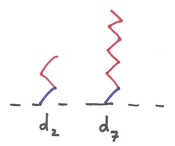
Figure 4.1: $2^{-2}$ and $2^{-7}$ in Hackenbush

Then we can easily verify that for all $n\geq 0$,

$$d_{n}\equiv\{0|d_{0},d_{1},\ldots,d_{n-1}\}.$$

So $d_{0}\equiv\{0|\}$, $d_{1}\equiv\{0|d_{0}\}$, $d_{2}\equiv\{0|d_{0},d_{1}\}$, and so on.

Then by the simplicity rule it easily follows inductively that $d_{n}\equiv\frac{1}{2^{n}}$. ∎

So we can assign a rational number to each Hackenbush position, describing the advantage that the position gives to Left or to Right. In many cases there are rules for finding these numbers, though there is probably no general rule, because the problem of determining the outcome of a general Hackenbush position is NP-hard, as shown on page 211-217 of Winning Ways.

4.4 The interplay of numbers and non-numbers

Unfortunately, not all games are numbers. However, the numbers play a fundamental role in understanding the structure of the other games.

First of all, they bound all other games:

Theorem 4.4.1.

Let $G$ be a game. Then there is some number $n$ such that $-n<G<n$.

Proof.

We show by induction that every game is less than a number.

Let $G$ be a game, and suppose that every option of $G$ is less than a number. Since all our games are short, $G$ has finitely many options. So we can find some $M$ such that every option $G^{L},G^{R}<M$. Without loss of generality, $M$ is a positive integer, so it has no right option. Then $G\leq M$ unless $G$ is $\geq$ a right option of $M$ (but none exist), or $M\leq$ a left option of $G$ (but we chose $M$ to exceed all options of $G$). Therefore $G\leq M$, by Theorem 3.3.7. Then $G<M+1$, and $M+1$ is a number. ∎

Because of this, we can examine which numbers are greater than or less than a given game.

Definition 4.4.2.

If $G$ is a game then we let $L(G)$ be the infimum (in $\mathbb{R}$) of all numbers $x$ such $G\leq x$, and $R(G)$ be the supremum of all numbers $x$ such that $x\leq G$.

These exist, because the previous theorem shows that the sets are non-empty, and because if $x\leq G$ for arbitrarily big $x$, then it could not be the case that $G<n$ for some fixed $n$.

It’s clear that $R(G)\leq L(G)$, since if $x\leq G$ and $G\leq y$, then $x\leq y$. It’s not yet clear that $R(G)$ and $L(G)$ must be dyadic rational numbers, but we will see this soon. If $G$ is a number, then clearly $R(G)=G=L(G)$. Another easily verified fact is that if $x$ is a number, then $L(G+x)=L(G)+x$ and $R(G+x)=R(G)+x$ for any $x$. Also, it’s easy to show that $L(G+H)\leq L(G)+L(H)$ and similarly that $R(G+H)\geq R(G)+R(H)$, using the fact that if $x\leq G$ and $y\leq H$, then $x+y\leq G+H$.

Numbers are games in which any move makes the game worse for the player who made the move. Such games aren’t very fun to play in, so Left and Right might decide to simply stop as soon as the state of the game becomes a number. Suppose they take this number as the final score of the game, with Left trying to maximize it, and Right trying to minimize it. Then the final score under perfect play is called the “stopping value.” Of course it depends on who goes first, so we actually get two stopping values:

Definition 4.4.3.

Let $G$ be a short game. We recursively define the left stopping value $LS(G)$ and the right stopping value $RS(G)$ by

• If $G$ equals a number $x$, then $LS(G)=RS(G)=x$.

• Otherwise, $LS(G)$ is the maximum value of $RS(G^{L})$ as $G^{L}$ ranges over the left options of $G$; and $RS(G)$ is the minimum value of $LS(G^{R})$ as $G^{R}$ ranges over the right options of $G$.

Then we have the following:

Theorem 4.4.4.

Let $G$ be a game and $x$ be a number. Then

• If $x>LS(G)$ then $x>G$.

• If $x<LS(G)$ then $x\lhd G$.

• If $x<RS(G)$ then $x<G$.

• If $x>RS(G)$ then $x\rhd G$.

Proof.

We proceed by joint induction on $G$ and $x$. As usual, we need no base case.

If $G$ equals a number, then all results are obvious. So suppose that $G$ is not equal to a number, so that $LS(G)$ is the maximum value of $RS(G^{L})$ and $RS(G)$ is the maximum value of $LS(G^{R})$. We have four things to prove.

Suppose $x>LS(G)$. Then since $G$ does not equal a number, we only need to show that $G\leq x$. This will be true unless $x^{R}\leq G$ for some $x^{R}$, or $x\leq G^{L}$ for some $G^{L}$. In the first case, we have $x^{R}>x>LS(G)$, so by induction $x^{R}>G$, not $x^{R}\leq G$. In the second case, note that $x>LS(G)\geq RS(G^{L})$ so by induction $x\rhd G^{L}$, not $x\leq G^{L}$.

Next, suppose that $x<LS(G)$. Then there is some $G^{L}$ such that $x<LS(G)=RS(G^{L})$. By induction, then $x<G^{L}$. So $x\leq G^{L}\lhd G$, and thus $x\lhd G$.

The cases where $x>RS(G)$ and $x<RS(G)$ are handled similarly. ∎

Corollary 4.4.5.

If $G$ is any short game, then $LS(G)=L(G)$ and $RS(G)=R(G)$.

Proof.

Clear from the definition of $L(G)$ and $R(G)$ and the previous theorem. ∎

Interestingly, this means that the left stopping value of any non-numerical game is at least its right stopping value

$$LS(G)\geq RS(G).$$

So in some sense, in a non-numerical game you usually want to be the first person to move. Since $LS(G)$ and $RS(G)$ are synonymous with $L(G)$ and $R(G)$, we drop the former and write $L(G)$ and $R(G)$ for the left stopping value and the right stopping value.

Using these results, we can easily compute $L(G)$ and $R(G)$ for various games. For $*=\{0|0\}$, the left and right stopping values are easily seen to be 0, so $L(*)=R(*)=0$. It follows that $*$ is less than every positive number and greater than every negative number. Such games are called infinitesimal or small games, and will be discussed more in a later section.

For another example, the game $\pm 1=\{1|-1\}$ has $L(\pm 1)=1$ and $R(\pm 1)$. So it is less than every number in $(1,\infty)$, and greater than every number in $(-\infty,1)$, but fuzzy with $(-1,1)$.

The next result formalizes the notion that “numbers aren’t fun to play in.”

Theorem 4.4.6.

(Number Avoidance Theorem) Let $x$ be a number and $G=\{G^{L}|G^{R}\}$ be a short game that does not equal any number. Then

$$G+x=\{G^{L}+x|G^{R}+x\}.$$

Proof.

Let $G_{x}=\{G^{L}+x|G^{R}+x\}$. Then consider

$$G_{x}-G=\{G_{x}-G^{R},(G^{L}+x)-G|G_{x}-G^{L},(G^{R}+x)-G\}.$$

Now for any $G^{R}$, $G^{R}+x$ is a right option of $G_{x}$, so $G^{R}+x\rhd G_{x}$ and therefore $G_{x}-G^{R}\lhd x$. Similarly, $G^{L}\lhd G$, so that $(G^{L}+x)-G\lhd x$ for every $G^{L}$. So every left option of $G_{x}-G$ is $\lhd x$.

Similarly, for any $G^{L}$, we have $G^{L}+x\lhd G_{x}$ so that $x\lhd G_{x}-G^{L}$. And for any $G^{R}$, $G\lhd G^{R}$ so that $x\lhd(G^{R}+x)-G$. So every right option of $G_{x}-G$ is $\rhd x$. Then by the simplicity rule, $G_{x}-G$ is a number, $y$. We want to show that $y=x$.

Note that $G_{x}=G+y$, so that

$$L(G_{x})=L(G)+y.$$ (4.2)

Now $y$ is a number and $G$ is not, so $G_{x}$ is not a number. Therefore $L(G_{x})$ is the maximum value of $R(G^{L}+x)=R(G^{L})+x$ as $G^{L}$ ranges over the left options of $G$. Since the maximum value of $R(G^{L})$ as $G^{L}$ ranges over the left options of $G$ is $L(G)$, we must have $L(G_{x})=L(G)+x$. Combining this with (4.2) gives $y=x$. So $G_{x}-G=x$ and we are done. ∎

This theorem needs some explaining. Some simple examples of its use are

$$*+x=\{x|x\}$$

and

$$\{-1|1\}+x=\{-1+x|1+x\}$$

for any number $x$. To see why it is called “Number Avoidance,” note that the definition of $G+x$ is

$$G+x=\{G^{L}+x,G+x^{L}|G^{R}+x,G+x^{R}\},$$

where the options $G+x^{L}$ and $G+x^{R}$ correspond to the options of moving in $x$ rather than in $G$. The Number Avoidance theorem says that such options can be removed without affecting the outcome of the game. The strategic implication of this is that if you are playing a sum of games, you can ignore all moves in components that are numbers. This works even if your opponent does move in a number, because by the gift-horse principle,

$$G+x=\{G^{L}+x|G^{R}+x,G+x^{R}\}$$

in this case.

4.5 Mean Value

If $G$ and $H$ are short games, then $L(G+H)\leq L(G)+L(H)$ and $R(G+H)\geq R(G)+R(H)$. It follows that the size of the confusion interval $[R(G+H),L(G+H)]$ is at most the sum of the sizes of the confusion intervals of $G$ and $H$.

Now if we add a single game to itself $n$ times, what happens in the limit? We might expect that $L(nG)-R(nG)$ will be approximately $n(L(G)-R(G))$. But in fact, the size of the confusion interval is bounded:

Theorem 4.5.1.

(Mean Value Theorem) Let $nG$ denote $G$ added to itself $n$ times. Then there is some bound $M$ dependent on $G$ but not $n$ such that

$$L(nG)-R(nG)\leq M$$

for every $n$.

Proof.

We noted above that

$$L(G+H)\leq L(G)+L(H).$$

But we can also say that

$$R(G+H)\leq R(G)+L(H)$$

for arbitrary $G$ and $H$, because if $x>R(G)$ and $y>L(H)$, then $x\rhd G$ and $y>H$, so that $x+y\rhd G+H$, implying that $x+y\geq R(G+H)$. Similarly,

$$L(G+H)\geq R(G)+L(H).$$

Every left option of $nG$ is of the form $G^{L}+(n-1)G$, and by these inequalities

$$R(G^{L}+(n-1)G)\leq L(G^{L})+R((n-1)G)$$

Therefore if we let $M_{1}$ be the maximum of $L(G^{L})$ over the left options of $G$, then

$$R(G^{L}+(n-1)G)\leq M_{1}+R((n-1)G)$$

and so every left option of $nG$ has right stopping value at most $M_{1}+R((n-1)G)$. Therefore $L(nG)\leq M_{1}+R((n-1)G)$.

Similarly, every right option of $nG$ is of the form $G^{R}+(n-1)G$, and we have

$$L(G^{R}+(n-1)G)\geq L(G^{R})+R((n-1)G)$$

Letting $M_{2}$ be the minimum value of $L(G^{R})$ over the right options of $G$, we have

$$L(G^{R}+(n-1)G)\geq M_{2}+R((n-1)G)$$

and so every right option of $nG$ has left stopping value at least $M_{2}+R((n-1)G)$. Therefore, $R(nG)\geq M_{2}+R((n-1)G)$.

Thus

$$L(nG)-R(nG)\leq M_{1}+R((n-1)G)-(M_{2}+R((n-1)G))=M_{1}-M_{2}$$

regardless of $n$. ∎

Together with the fact that $L(G+H)\leq L(G)+L(H)$ and $R(G+H)\geq R(G)+R(H)$ and $L(G)\geq R(G)$, it implies that

$$\lim_{n\to\infty}\frac{L(nG)}{n}\textrm{ and }\lim_{n\to\infty}\frac{R(nG)}{n}$$

converge to a common limit, called the mean value of $G$, denoted $m(G)$. It is also easily seen that $m(G+H)=m(G)+m(H)$ and $m(-G)=-m(G)$, and that $G\geq H$ implies $m(G)\geq m(H)$. The mean value of $G$ can be thought of as a numerical approximation to $G$.

Chapter 5 Games near 0

5.1 Infinitesimal and all-small games

As noted above, the game $*$ lies between all the positive numbers and all the negative numbers. Such games are called infinitesimals or small games.

Definition 5.1.1.

A game is infinitesimal (or small) if it is less than every positive number and greater than every negative number, i.e., if $L(G)=R(G)=0$. A game is all-small in form if every one of its positions (including itself) is infinitesimal. A game is all-small in value if it equals an all-small game.

Since $L(G+H)\leq L(G)+L(H)$ and $R(G+H)\geq R(G)+R(H)$ and $R(G)\leq L(G)$, it’s clear that infinitesimal games are closed under addition. An easy inductive proof shows that all-small games are also closed under addition: if $G$ and $H$ are all-small in form, then every option of $G+H$ is all-small by induction, and $G+H$ is infinitesimal itself, so $G+H$ is all-small. Moreover, if $G$ is all-small in value, then the canonical value of $G$ is all-small in form.

Their name might suggest that all-small games are the smallest of games, but as we will see this is not the case: the game $+_{2}=\{0|\{0|-2\}\}$ is smaller than every positive all-small game.

Infinitesimal games occur naturally in certain contexts. For example, every position in Clobber is infinitesimal. To see this, let $G$ be a position in Clobber. We need to show that for any $n$,

$$\frac{-1}{2^{n}}\leq G\leq\frac{1}{2^{n}}.$$

As noted in the proof of Theorem 4.3.3, $\frac{1}{2^{n}}$ is a Hackenbush position consisting of string of edges attached to the ground: $1$ blue edge followed by $n$ red edges (see Figure 4.1). By symmetry, we only need to show that $G\leq\frac{1}{2^{n}}$, or in other words, that $\frac{1}{2^{n}}-G$ is a win for Left when Right goes first. Left plays as follows: whenever it is Left’s turn, she makes a move in $G$, unless there are no remaining moves in $G$. In this case there are no moves for Right either. This can be seen from the rules of Clobber - see Figure 5.1.

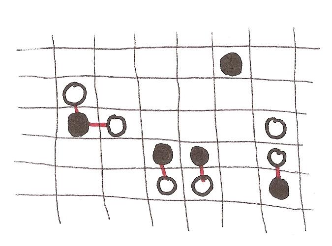
Figure 5.1: In a position of Clobber, whenever one player has available moves, so does the other. The available moves for each player correspond to the pairs of adjacent black and white pieces, highlighted with red lines in this diagram.

So once the game reaches a state where no more moves remain in $G$, Left can make the final move in $\frac{1}{2^{n}}$, by cutting the blue edge at the base of the stalk. This ends the other component.

In other words, the basic reason why Left can win is that she retains the ability to end the Hackenbush position at any time, and there’s nothing that Right can do about it.

Now since every subposition of a Clobber position is itself a Clobber position, it follows that Clobber positions are in fact all-small.

The only property of Clobber that we used was that whenever Left can move, so can Right, and vice versa. So we have the following

Theorem 5.1.2.

If $G$ is a game for which Left has options iff Right has options, and the same holds of every subposition of $G$, then $G$ is all-small.

Conversely

Theorem 5.1.3.

If $G$ is an all-small game in canonical form, then $G$ has the property that Left can move exactly when Right can, and this holds in all subpositions.

Proof.

By induction, we only need to show that this property holds for $G$. Suppose that it didn’t, so that $G=\{L|\emptyset\}$ or $G=\{\emptyset|R\}$. In the first case, there is some number $n$ such that $n$ exceeds every element of $L$. Therefore by the simplicity rule, $G$ is a number. Since $G$ is infinitesimal, it must be zero, but the canonical form of $0$ has no left options. So $G$ cannot be of the form $\{L|\emptyset\}$. The other possibility is ruled out on similar grounds. ∎

The entire collection of all-small games is not easy to understand. In fact, we will see later that there is an order-preserving homomorphism from the group $\mathcal{G}$ of (short) games into the group of all-small games. So all-small games are as complicated as games in general.

Here are the simplest all-small games:

$$0=\{|\}$$

$$*=\{0|0\}$$

$$\uparrow=\{0|*\}$$

$$\downarrow=\{*|0\}$$

The reader can easily check that $\uparrow>0$ but $\uparrow||*$. As an exercise in reducing to canonical form, the reader can also verify that

$$\uparrow+*=\{0,*|0\}$$

$$\uparrow+\uparrow=\{0|\uparrow+*\}$$

$$\uparrow+\uparrow+*=\{0|\uparrow\}$$

$$\{\uparrow|\downarrow\}=*$$

Usually we use the abbreviations $\uparrow*=\uparrow+*$, $\Uparrow=\uparrow+\uparrow$, $\Downarrow=\downarrow+\downarrow$, $\Uparrow*=\Uparrow+*$. More generally, $\hat{n}$ is the sum of $n$ copies of $\uparrow$ and $\hat{n}*=\hat{n}+*$.

These games occur in Clobber as follows:

Theorem 5.1.4.

Letting $\mu_{1}=\uparrow$, $\mu_{n+1}=\{0|\mu_{n}\}$, and $\nu_{1}=\uparrow*$, $\nu_{n+1}=\{0|\nu_{n}\}$, we have $\mu_{n+1}=\uparrow+\nu_{n}$ and $\nu_{n+1}=\uparrow+\mu_{n}$ and $\mu_{n+1}=\nu_{n+1}+*$ for every $n\geq 1$.

Proof.

We proceed by induction on $n$. The base case is already verified above in the examples. Otherwise

$$\uparrow+\nu_{n}=\{0|*\}+\{0|\nu_{n-1}\}=\{\uparrow,\nu_{n}|\uparrow+\nu_{n-1},\nu_{n}+*\}.$$

By induction, this is

$$\{\uparrow,\nu_{n}|\mu_{n},\mu_{n}\}$$

This value is certainly $\geq\{0|\mu_{n}\}$, since it is obtained by improving a left option ($0\to\uparrow$) and adding a left option of $\nu_{n}$. So it remains to show that $\mu_{n+1}=\{0|\mu_{n}\}\leq\{\uparrow,\nu_{n}|\mu_{n}\}$. This will be true unless $\mu_{n+1}\geq\mu_{n}$ (impossible, since $\mu_{n}$ is a right option of $\mu_{n+1}$), or $\{\uparrow,\nu_{n}|\mu_{n}\}\leq 0$ (impossible because Left can make an initial winning move to $\uparrow$). So $\uparrow+\nu_{n}=\mu_{n+1}$.

A completely analogous argument shows that $\uparrow+\mu_{n}=\nu_{n+1}$. Then for the final claim, note that $\mu_{n+1}=\uparrow+\nu_{n}=\uparrow+\mu_{n}-*=\uparrow+\mu_{n}+*=\nu_{n+1}+*$. ∎

So then $\mu_{2k-1}$ is the sum of $2k-1$ copies of $\uparrow$ and $\nu_{2k}$ is the sum of $2k$ copies of $\uparrow$, because $*+*=0$.

Using this, we get the following values of clobber positions:

We also can use this to show that the multiples of $\uparrow$ are among the largest of (short) infinitesimal games:

Theorem 5.1.5.

Let $G$ be a short infinitesimal game. Then there is some $N$ such that for $n>N$, $G\leq\mu_{n}$ and $G\leq\nu_{n}$. In particular, every infinitesimal game lies between two (possibly negative) multiples of $\uparrow$.

Proof.

Take $N$ to be larger than five plus the number of positions in $G$. We give a strategy for Left to use as the second player in $\mu_{n}-G$. The strategy is to always move to a position of the form $\mu_{m}+H$, where $m>5$ and $R(H)\geq 0$, until the very end. The initial position is of this form. From such a position, Right can only move to $\mu_{m-1}+H$ or to $\mu_{m}+H^{R}$ for some $H$. In the first case, we use the fact that $L(H)\geq R(H)\geq 0$, and find a left option $H^{L}$ such that $R(H^{L})\geq 0$. Then $\mu_{m-1}+H^{L}$ is of the desired form. In the other case, since $R(H)\geq 0$, $L(H^{R})\geq 0$, and therefore we can find some $H^{RL}$ such that $R(H^{RL})\geq 0$. We make such a move. Left uses this strategy until $H$ becomes a number.

Note that if we follow this strategy, we (Left) never move in the $\mu_{n}$ component. Therefore, the complexity of the other component will decrease after each of our turns. By the time that $H$ becomes a number $x$, we will stil lbe in a position $\mu_{m}+x$ with $m$ at least four or five, by choice of $n$.

Now by following our strategy, once $H$ becomes a number, the number will be nonnegative. So we will be in a position $\mu_{m}+x$, where $x\geq 0$ and $m$ is at least four or five. Either Left or Right moved to this position. Either way, this position is positive (because $x\geq 0$ and $\mu_{m}>0$ for $m>1$), so therefore Left wins.

The same argument shows that $\nu_{n}-G$ is positive for sufficiently large $n$.

Since the positive multiples of $\uparrow$ are of the form $\mu_{n}$ or $\nu_{n}$, all sufficiently large multiples of $\uparrow$ will exceed $G$. By the same logic, all sufficiently large negative multiples of $\uparrow$ (i.e., multiples of $\downarrow$) will be less than $G$. So our claim is proven. ∎

We end this section by showing that some infinitesimal games are smaller than all positive all-small games. For any positive number $x$, let $+_{x}$ (pronounced “tiny $x$”) be the game $\{0||0|-x\}\equiv\{0|\{0|-x\}\}$. The negative of $+_{x}$ is $\{x|0||0\}$, which we denote $-_{x}$ (pronounced “miny $x$”).

Theorem 5.1.6.

For any positive number $x$, $+_{x}$ is a positive infinitesimal, and $+_{x}<G$ for any positive all-small $G$. Also, if $G$ is any positive infinitesimal, then $+_{x}<G$ for sufficiently large $x$.

Proof.

It’s easy to verify that $L(+_{x})=R(+_{x})=0$, and that $+_{x}>0$.

For the first claim, let $G$ be a positive all-small game. We need to show that $G+(-_{x})$ is still positive. If Left goes first, she can win by making her first move be $\{x|0\}$. Then Right is forced to respond by moving to $0$ in this component, or else Left can move to $x$ on her next turn, and win (because $x$ is a positive number, so that $x$ plus any all-small game will be positive). So Right is forced to move to $0$. This returns us back to $G$ alone, which Left wins by assumption.

If Left goes second, then she follows the same strategy, moving to $\{x|0\}$ at the first moment possible. Again, Right is forced to reply by moving $\{x|0\}\to 0$, and the brief interruption has no effect. The only time that this doesn’t work is if Right’s first move is from $-_{x}$ to $0$. This leaves $G+0$, but Left can win this since $G>0$. This proves the first claim.

For the second claim, we use identical arguments, but choose $x$ to be so large that $-x<G^{*}<x$ for every position $G^{*}$ occurring anywhere within $G$. Then Left’s threat to move to $x$ is still strong enough to force a reply from Right. ∎

So just as the multiples of $\uparrow$ are the biggest infinitesimal games, the games $+_{x}$ are the most miniscule.

5.2 Nimbers and Sprague-Grundy Theory

An important class of all-small games is the nimbers

$$*n=\{*0,*1,\ldots,*(n-1)\}$$

where we are using $\{A\}$ as shorthand for $\{A|A\}$. For instance

$$*0=\{|\}=0$$

$$*1=\{0|0\}=*$$

$$*2=\{0,*|0,*\}$$

$$*3=\{0,*,*2|0,*,*2\}$$

These games are all-small by the same criterion that made Clobber games all-small. Note that if $m<n$, then $*n$ has $*m$ as both a left and a right option, so $*m\lhd*n\lhd*m$. Thus $*m||*n$. So the nimbers are pairwise distinct, and in fact pairwise fuzzy with each other.

There are standard shorthand notations for sums of numbers and nimbers:

$$x*n\equiv x+*n$$

$$x*\equiv x+*1\equiv x+*$$

where $x$ is a number and $n\in\mathbb{Z}$. Similarly, $7\uparrow$ means $7+\uparrow$ and so on.This notation is usually justified as an analog to mixed fraction notation like $5\frac{1}{2}$ for $\frac{11}{2}$.

Because nimbers are infinitesimal, we can compare expressions of this sort as follows: $x_{1}*n_{1}\leq x_{2}*n_{2}$ if and only if $x_{1}<x_{2}$, or $x_{1}=x_{2}$ and $n_{1}=n_{2}$. We will see how to add these kind of values soon.

The nimbers are so-called because they occur in the game Nim. In fact, the nim-pile of size $n$ is identical to the nimber $*n$.

Nim is an example of an impartial game, a game in which every position is its own negative. In other words, every left option of a position is a right option, and vice versa. When working with impartial games, we can use “option” without clarifying whether we mean left or right option. The impartial games are exactly those which can be built up by the operation $\{A,B,C,\ldots|A,B,C,\ldots\}$, in which we require the left and right sides of the $|$ to be the same. This is often abbreviated to $\{A,B,C,\ldots\}$, and we use this abbreviation for the rest of the section.

Another impartial game is Kayles. Like Nim, it is played using counters in groups. However, now the counters are in rows, and a move consists of removing one or two consecutive counters from a row. Doing so may split the row into two pieces. Both players have the same options, and as usual we play this game using the normal play rule, where the last player to move is the winner.

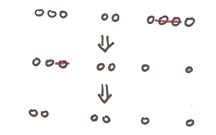
Figure 5.2: Two moves in a game of Kayles. Initially there are rows of length 3, 2, and 4. The first player splits the row of 4 into rows of length 1 and 1, by removing the middle two pieces. The second player reduces the row of length 3 to length 2.

So if $K_{n}$ denotes the Kayles-row of length $n$, then we have

$$K_{1}=\{0\}=*$$

$$K_{2}=\{0,K_{1}\}$$

$$K_{3}=\{K_{1},K_{2},K_{1}+K_{1}\}$$

$$K_{4}=\{K_{2},K_{1}+K_{1},K_{3},K_{2}+K_{1}\}$$

$$K_{5}=\{K_{3},K_{2}+K_{1},K_{4},K_{3}+K_{1},K_{2}+K_{2}\}$$

Another similar game is Grundy’s game. This game is played with piles, like Nim, but rather than removing counters, the move is to split a pile into two non-equal parts. So if $G_{n}$ denotes a Grundy-heap of size $n$, then

$$G_{1}=\{\}=0$$

$$G_{2}=\{\}=0$$

$$G_{3}=\{G_{1}+G_{2}\}$$

$$G_{4}=\{G_{1}+G_{3}\}$$

$$G_{5}=\{G_{1}+G_{4},G_{2}+G_{3}\}$$

$$G_{6}=\{G_{1}+G_{5},G_{2}+G_{4}\}$$

$$G_{7}=\{G_{1}+G_{6},G_{2}+G_{5},G_{3}+G_{4}\}$$

and so on.

The importance of nimbers is the following:

Theorem 5.2.1.

Every impartial game equals a nimber.

Proof.

Because of how impartial games are constructed, it inductively suffices to show that if all options of an impartial game are nimbers, then the game itself is a nimber. This is the following lemma: ∎

Lemma 5.2.2.

If $a,b,c,\ldots$ are nonnegative integers, then

$$\{*a,*b,*c,\ldots\}=*m,$$

where $m$ is the smallest nonnegative integer not in the set $\{a,b,c,\ldots\}$, the minimal excludent of $a,b,c,\ldots$.

Proof.

Since impartial games are their own negatives, we only need to show that $*m\leq x=\{*a,*b,*c,\ldots\}$. This will be true unless $*m\geq$ an option of $x$ (impossible since $*m||*a,*b,*c,\ldots$ because $m\neq a,b,c,\ldots$), or if $x\leq$ an option of $*m$. But by choice of $*m$, every option of $*m$ is an option of $x$, so $x$ is incomparable with every option of $*m$. Thus this second case is also impossible, and so $*m\leq x$. ∎

One can easily show that the sum of two impartial games is an impartial game. So which nimber is $*m+*n$?

Lemma 5.2.3.

If $m,n<2^{k}$, then $*m+*(2^{k})=*(m+2^{k})$, and $*m+*n=*q$ for some $q<2^{k}$.

Proof.

We proceed by induction on $k$. The base case $k=0$ is true because $*0=0$ and so $*0+*0=*0$ and $*0+*(2^{0})=*(0+2^{0})$.

So suppose the hypothesis is true for $k$. Let $m,n<2^{k+1}$. We can write $m=m^{\prime}+i2^{k}$ and $n=n^{\prime}+j2^{k}$, where $i,j\in\{0,1\}$ and $m^{\prime},n^{\prime}<2^{k}$. Then by induction,

$$*m=*m^{\prime}+*(i2^{k})$$

$$*n=*n^{\prime}+*(j2^{k})$$

$$*m+*n=*q^{\prime}+*(i2^{k})+*(j2^{k})$$

where $*q^{\prime}=*m^{\prime}+*n^{\prime}$, and $q^{\prime}<2^{k}$. Now $i2^{k}$ is either $0$ or $2^{k}$ and similarly for $j2^{k}$, so the correction term $*(i2^{k})+*(j2^{k})$ is either $*0+*0=*0$, $*0+*2^{k}=*2^{k}$, or $*2^{k}+*2^{k}=*0$ (using the fact that impartial games are their own inverses).

So $*m+*n$ is either $*q^{\prime}$ where $q^{\prime}<2^{k}<2^{k+1}$, in which case we are done, or $*q^{\prime}+*2^{k}$, which by induction is $*(q^{\prime}+2^{k})$. Then we are done since $q^{\prime}+2^{k}<2^{k+1}$.

So if $m,n<2^{k+1}$, then $*m+*n=*q$ for some $q<2^{k+1}$. Since addition of games (modulo equality) is cancellative and associative, it follows that $\{*q:q<2^{k+1}\}$ forms a group.

It remains to show that for any $m<2^{k+1}$, $*m+*2^{k+1}=*(m+2^{k+1})$. We show this by induction on $m$ ($k$ is fixed of course). The options of $*m+*2^{k+1}$ are of two forms:

• $*m+*n$ for $n<2^{k+1}$. Because $\{*q\,:\,q<2^{k+1}\}$ with addition forms a group, $\{*m+*n\,:\,n<2^{k+1}\}=\{*n\,:\,n<2^{k+1}\}$.

• $*m^{\prime}+*2^{k+1}$ for $m^{\prime}<2^{k+1}$. By induction, this is just $\{*(m^{\prime}+2^{k+1})\,:\,m^{\prime}<m\}$.

So all together, the options of $*m+*2^{k+1}$ are just

$$\{*n\,:\,n<2^{k+1}\}\cup\{*n\,:\,2^{k+1}\leq n<2^{k+1}+m\}=\{*0,*1,\ldots,*(2^{k+1}+m-1)\}.$$

Therefore the minimal excludent is $m+2^{k+1}$, and so $*m+*2^{k+1}=*(m+2^{k+1})$. ∎

Together with the fact that $*m+*m=0$, we can use this to add any two nimbers:

$$*9+*7=(*1+*8)+(*3+*4)=(*1+*8)+(*1+*2+*4)=$$

$$(*1+*1)+*2+*4+*8=0+*2+*4+*8=*6+*8=*14.$$

$$*25+*14=(*1+*8+*16)+(*2+*4+*8)=*1+*2+*4+(*8+*8)+*16=$$

$$*1+*2+*4+*16=*23.$$

In general, the approach is to split up the summands into powers of two, and them combine and cancel out like terms. The reader can show that the general rule for $*m+*n$ is to write $m$ and $n$ in binary, and add without carries, to produce a number $l$ which will satisfy $*m+*n=*l$.

The number $l$ such that $*m+*n=*l$ is called the nim-sum of $m$ and $n$, denoted $m+_{2}n$. Here is an addition table:

$+_{2}$	0	1	2	3	4	5	6	7
0	0	1	2	3	4	5	6	7
1	1	0	3	2	5	4	7	6
2	2	3	0	1	6	7	4	5
3	3	2	1	0	7	6	5	4
4	4	5	6	7	0	1	2	3
5	5	4	7	6	1	0	3	2
6	6	7	4	5	2	3	0	1
7	7	6	5	4	3	2	1	0

Note also that sums of numbers and nimbers are added as follows: $x*n+y*m=(x+y)*(n+_{2}m)$.

Using nim-addition and the minimal-excludent rule, we can calculate values of some positions in Kayles and Grundy

$$K_{1}=\{0\}=*$$

$$K_{2}=\{0,K_{1}\}=\{0,*\}=*2$$

$$K_{3}=\{K_{1},K_{2},K_{1}+K_{1}\}$$

$$=\{*,*2,*+*\}=\{*,*2,0\}=*3$$

$$K_{4}=\{K_{2},K_{1}+K_{1},K_{3},K_{2}+K_{1}\}$$

$$=\{*2,*+*,*3,*2+*1\}=\{*2,0,*3,*3\}=*$$

$$K_{5}=\{K_{3},K_{2}+K_{1},K_{4},K_{3}+K_{1},K_{2}+K_{2}\}$$

$$=\{*3,*2+*1,*,*3+*1,*2+*2\}=\{*3,*3,*,*2,*0\}=*4$$

$$G_{1}=\{\}=0$$

$$G_{2}=\{\}=0$$

$$G_{3}=\{G_{1}+G_{2}\}=\{0+0\}=*$$

$$G_{4}=\{G_{1}+G_{3}\}=\{0+*\}=0$$

$$G_{5}=\{G_{1}+G_{4},G_{2}+G_{3}\}$$

$$=\{0+0,0+*\}=\{0,*\}=*2$$

$$G_{6}=\{G_{1}+G_{5},G_{2}+G_{4}\}$$

$$=\{0+*2,0+0\}=\{0,*2\}=*$$

$$G_{7}=\{G_{1}+G_{6},G_{2}+G_{5},G_{3}+G_{4}\}$$

$$=\{0+*,0+*2,*\}=\{*,*2\}=0$$

In general, there are sequences of integers $\kappa_{n}$ and $\gamma_{n}$ such that $K_{n}=*\kappa_{n}$ and $G_{n}=*\gamma_{n}$. One can construct a table of these values, and use it to evaluate any small position in Grundy’s game or Kayles. For the case of Kayles, this sequence is known to become periodic after the first hundred or so values, but for Grundy’s game periodicity is not yet know to occur.

The theory of impartial games is called Sprague-Grundy theory, and was the original form of additive CGT which Conway, Guy, Berlekamp and others extended to handle partizan games.

Chapter 6 Norton Multiplication and Overheating

6.1 Even, Odd, and Well-Tempered Games

Definition 6.1.1.

A short game $G$ is even in form if every option is odd in form, and odd in form if every option is even in form and $G\neq 0$. $G$ is even (odd) in value if it equals a short game that is even (odd) in form.

For instance

• $0=\{|\}$ is even and not odd (in form).

• $*=\{0|0\}$ and $1=\{0|\}$ are odd and not even (in form).

• $2=\{1|\}$ is even and not odd (in form).

• $2=\{0,1|\}$ is neither even nor odd (in form), but even (in value).

• In general an integer is even or odd in value if it is even or odd in the usual sense.

• $1/2=\{0|1\}$ is neither even nor odd (in form). By (b) of the following theorem, it is neither even nor odd in value, too.

Theorem 6.1.2.

Let $G$ be a short game.

(a)

If $G$ is a short game that is odd (even) in form, then the canonical form of $G$ is also odd (even) in form.

(b)

$G$ is even or odd (in value) iff the canonical form of $G$ is even or odd (in form)

(c)

$G$ is even or odd (in form) iff $-G$ is even or odd (in form). $G$ is even or odd (in value) iff $-G$ is even or odd (in value).

(d)

No game is both even and odd (in form or in value).

(e)

The sum of two even games or two odd games is even. The sum of an odd game and an even game is an odd game. True for forms or values.

(f)

If every option of $G$ is even (or odd) in value, and $G\neq 0$, then $G$ is odd (or even) in value.

Proof.

(a)

Let $G$ be odd or even in form. By induction we can put all the options of $G$ in canonical form. We can then reduce $G$ to canonical form by bypassing reversible options and removing dominated options. None of these operations will introduce options of $G$ of the wrong parity: this is obvious in the case of removing dominated options, and if, say, $G^{R}$ is a reversible option reversed by $G^{RL}$, then $G^{R}$ has the opposite parity of $G$, and $G^{RL}$ has the same parity as $G$, so that every left option of $G^{RL}$ has opposite parity of $G$, and can be added to the list of options of $G$ without breaking the parity constraint. Of course since removing dominated moves and bypassing reversible moves does not effect the value of $G$, the constraint that $G\neq 0$ when $G$ is odd will never be broken. So after reducing $G$ to canonical form, it will still be odd or even, as appropriate.

(b)

If $G$ is, say, odd in value, then $G=H$ for some $H$ that is odd in form. Letting $H^{\prime}$ be the canonical form of $H$, by part (a) $H^{\prime}$ is odd (in form). Since $H^{\prime}$ is also the canonical form of $G$, we see that the canonical form of $G$ is odd (in form). Conversely, if the canonical form of $G$ is odd (in form), then $G$ is odd in value by definition, since $G$ equals its canonical form.

(c)

Clear by induction - the definitions of even and odd are completely symmetric between the two players.

(d)

We first show that no game is both even and odd in form, by induction. Let $G$ be a short game, and suppose it is both even and odd in form. Then by definition, every option of $G$ is both even and odd in form. By induction, $G$ has no options, so $G\equiv\{|\}=0$, and then $G$ is not odd.

Next, suppose that $G$ is both even and odd in value. Then by part (b), the canonical form of $G$ is both even and odd in form, contradicting what we just showed.

(e)

We first prove the two statements about even and odd games in form, by induction. Suppose that both $G$ and $H$ have parities in form. By induction, every option of $G+H$ will have the correct parity. So we only need to show that if $G$ is odd and $H$ is even (or vice versa), then $G+H\neq 0$. But if $G+H=0$, then $G=-H$, and since $H$ is even, so is $-H$, by part (c), so we have a contradiction of part (d), since $G$ is odd and $-H$ is even.

Now suppose that $G$ and $H$ are both even or odd (in value). Then $G=G^{\prime}$ and $H=H^{\prime}$, for some games $G^{\prime}$ and $H^{\prime}$ having the same parities (in form) as $G$ and $H$ have (in value). Then $G+H=G^{\prime}+H^{\prime}$, and $G^{\prime}+H^{\prime}$ has the desired parity (in form), so $G+H$ has the desired parity (in value).

(f)

For every option of $G$, there is an equivalent game having the same parity, in form. Assembling these equivalent games into another game $H$, we have $G=H$ by Theorem 3.3.6(c), and $H$ has the desired parity (in form), so $G$ has the desired parity (in value).

∎

Henceforth “even” and “odd” will mean even and odd in value. From this theorem, we see that the even and odd values form a subgroup of $\mathcal{G}$ (the group of short games), with the even values as an index 2 subgroup. Every even or odd game can be uniquely written as an even game plus an element of the order-2 subgroup $\{0,*\}$, because $*$ is odd and has order 2.

Later, using Norton multiplication, we’ll see that the group of (short) even games is isomorphic as a partially-ordered group to the entire group $\mathcal{G}$ of short games.

A slight variation of even and odd is even and odd -temper:

Definition 6.1.3.

Let $G$ be a short game. Then $G$ is even-tempered in form if it equals a (surreal) number, or every option is odd-tempered in form. Similarly, $G$ is odd-tempered in form if does not equal a number, and every option is even-tempered in form. Also, $G$ is odd- (even-)tempered in value if it equals a short game that is odd or even tempered in form.

This notion behaves rather differently: now $0,1,1/2$ are all even-tempered, while $*,1*,$ and $\{1|0\}$ are odd-tempered, and $\uparrow$ is neither. Intuitively, a game is even- or odd-tempered iff a number will be reached in an even- or odd- number of moves.

We say that a game is well-tempered if it is even-tempered or odd-tempered.

Theorem 6.1.4.

If $G$ is a short game that is odd- or even-tempered in form, then the canonical form of $G$ is also odd- or even-tempered in form.

$G$ is even- or odd-tempered (in value) iff the canonical form of $G$ is even- or odd-tempered (in form).

Then $G$ is even- or odd-tempered (in form) iff $-G$ is even- or odd-tempered (in form). $G$ is even- or odd-tempered (in value) iff $-G$ is even- or odd-tempered (in value).

If $G$ is even- or odd-tempered (in value), then so is $G+x$, for any number $x$.

No game is both even- and odd-tempered (in form or in value).

The sum of two even-tempered games or two odd-tempered games is even-tempered. The sum of an odd-tempered game and an even-tempered game is an odd-tempered game. True in values (not forms).

If $G$ does not equal a number, and every option of $G$ is even- or odd-tempered in value, then $G$ is odd- or even-tempered in value.

Proof.

Most of the proofs are the same as in the case for even and odd games. However, we have the following subtleties:

(a)

When bypassing reversible moves, we now need to check that the replacement options $G^{RLR}$ actually have the appropriate parity. If $G$ itself equals a number, then the parity of the bypassed options is irrelevant. Otherwise, if $G^{R}$ equals a number, then since we’ve reduced to canonical form, $G^{RL}$ and $G^{RLR}$ will also be numbers, so they will have the same temper as $G^{R}$, and everything works out fine.

The only possible failure case is when $G^{RL}$ is a number, so every one of its left options $G^{RLR}$ is even tempered, and $G$ and $G^{R}$ are even- and odd-tempered non-numerical games, respectively. Since $G^{RL}\geq G$ (by definition of reversible move), $G^{RL}$ must be greater than or fuzzy with every left option of $G$. If $G^{RL}$ were additionally less than or fuzzy with every right option of $G$, then by the simplicity rule $G$ would be a number. So some right option $H$ of $G$ must be less than or equal to $G^{RL}$. This option cannot be $G^{R}$ itself, since $G^{RL}\lhd G^{R}$. So $H$ will remain a right option of $G$ after bypassing $G^{R}$. But then $H\leq G^{RL}\leq G^{RLR}$ for every new option $G^{RLR}$. Here $G^{RL}\leq G^{RLR}$ because $G^{RL}$ is a number. So all the new moves will be dominated by $H$ and can be immediately discarded, fixing the problem.

(b-c)

These remain true for identical reasons as for even and odd games.

(c’)

Suppose $G$ is even tempered (in value). Then it equals a game $H$ that is even-tempered (in form). If $G$ equals a number, then so does $G+x$, so $G+x$ is also even-tempered (in form and value). Otherwise, $H$ does not equal a number, so by number avoidance

$$H+x=\{H^{L}+x|H^{R}+x\}.$$

By induction, every $H^{L}+x$ and $H^{R}+x$ is odd-tempered in value, so by part (f), $H+x$ is even-tempered in value.

Similarly, if $G$ is odd tempered in value, then it equals a game $H$ that is odd-tempered (in form). And since $G$ and $H$ are not equal to numbers, neither is $G+x$, so it suffices to show that every option of $\{H^{L}+x|H^{R}+x\}$ is even-tempered in value, which follows by induction.

(d)

The proof that no game is both even- and odd-tempered in form is essentially the same: unless $G$ is a number, $G$ can have no options by induction, and then it equals zero and is not odd. And if $G$ is a number, then $G$ is not odd in form. Extending this result to values proceeds in the same way as before, using part (a).

(e)

Note that this is not true in forms, since $1+*=\{*,1|1\}$, and $*$ and $1$ are odd- and even-tempered respectively, so that $\{*,1|1\}$ is neither even- nor odd-tempered in form. But it equals $\{1|1\}$ which is odd-tempered in form, so it is odd-tempered in value.

We prove the result for values inductively, making use of part (f). If $G$ and $H$ are even or odd-tempered games, then every option of $G+H$ will have the desired temper (in value), except when one of $G$ or $H$ is a number. But this case follows from part (c’). So the only remaining thing we need to show is that if $G$ and $H$ are even- and odd-tempered in value, respectively, then $G+H$ is not a number. But if $G+H=x$ for some number $x$, then $G=x+(-H)$, so by parts (c-c’), $x+(-H)$ is odd-tempered in value. But then $G$ is both even- and odd-tempered in value, contradicting part (d).

(f)

This proceeds as in the previous theorem.

∎

So as in the previous case, even and odd-tempered values form a subgroup of $\mathcal{G}$, with the even-tempered games as an index 2 subgroup, having $\{0,*\}$ as a complement. But in this case, something more interesting happens: the group of all short games is a direct sum of even-tempered games and infinitesimal games.

Theorem 6.1.5.

Every short partizan game $G$ can be uniquely written as $E+\epsilon$, where $E$ is even-tempered and $\epsilon$ is infinitesimal.

To prove this, we need some preliminary definitions and results:

Definition 6.1.6.

If $G$ and $H$ are games, we say that $G$ is $H$-ish if $G-H$ is an infinitesimal.

Since infinitesimals form a group, this is an equivalence relation. The suffix “-ish” supposedly stands for “infinitesimally shifted,” though it also refers to the fact that $G$ and $H$ are approximately equal. For instance, they will have the same left and right stopping values. We can rephrase Theorem 6.1.5 as saying that every short game is even-tempered-ish.

Lemma 6.1.7.

If $G=\{A,B,\ldots|C,D,\ldots\}$ is a short game that does not equal a number, and $A^{\prime}$ is $A$-ish, $B^{\prime}$ is $B$-ish, and so on, then

$$G^{\prime}=\{A^{\prime},B^{\prime},\ldots|C^{\prime},D^{\prime},\ldots\}$$

is $G$-ish.

Proof.

Since $G$ does not equal a number, we know by number avoidance that for every positive number $\delta$,

$$G+\delta=\{A+\delta,B+\delta,\ldots|C+\delta,D+\delta,\ldots\}$$

But since $A^{\prime}$ is $A$-ish, $A^{\prime}-A\leq\delta$, and $B^{\prime}-B\leq\delta$, and so on, so that $A^{\prime}\leq A+\delta$, $B^{\prime}\leq B+\delta$, and so on. Therefore,

$$G^{\prime}=\{A^{\prime},B^{\prime},\ldots|C^{\prime},D^{\prime},\ldots\}\leq\{A+\delta,B+\delta,\ldots,C+\delta,D+\delta,\ldots\}=G+\delta.$$

So $G^{\prime}-G\leq\delta$ for every positive number $\delta$. Similarly, $G^{\prime}-G\geq\delta$ for every negative number $\delta$, so that $G^{\prime}-G$ is infinitesimal. ∎

Corollary 6.1.8.

For every short game $G$, there are $G$-ish even-tempered and odd-tempered games.

Proof.

We proceed by induction on $G$. If $G$ is a number, then $G$ is already even-tempered, and $G+*$ is odd-tempered and $G$-ish because $*$ is infinitesimal. If $G$ is not a number, let $G=\{A,B,\ldots|C,D,\ldots\}$. By induction, there are odd-tempered $A^{\prime}$, $B^{\prime}$, …such that $A^{\prime}$ is $A$-ish, $B^{\prime}$ is $B$-ish, and so on. By the lemma,

$$G^{\prime}=\{A^{\prime},B^{\prime},\ldots|C^{\prime},D^{\prime},\ldots\}$$

is $G$-ish. It is also even-tempered in value, by part (f) of Theorem 6.1.4, unless $G^{\prime}$ is a number. But then it is even-tempered in form and value, by definition of even-tempered. So either way $G^{\prime}$ is even-tempered and $G$-ish. Then as before, $G+*$ is odd-tempered and also $G$-ish. ∎

It remains to show that $0$ is the only even-tempered infinitesimal game.

Theorem 6.1.9.

Let $G$ be an even or even-tempered game. If $R(G)\geq 0$, then $G\geq 0$. Similarly, if $L(G)\leq 0$, then $G\leq 0$.

Proof.

By symmetry we only need to prove the first claim. Since right and left stopping values depend only on value, not form, we can assume without loss of generality that $G$ is even or even-tempered in form. We proceed by induction. If $G$ equals a number, then $R(G)=G$ and we are done. Otherwise, every option of $G$ is odd or odd-tempered in form, and we have

$$L(G^{R})\geq R(G)\geq 0$$

for all $G^{R}$, by definition of stopping values. We need to show that Left wins $G$ when Right goes first. Suppose for the sake of contradiction that Right wins, and let $G^{R}$ be Right’s winning move. So $G^{R}\leq 0$. If $G^{R}$ is a number, then

$$0\leq L(G^{R})=G^{R}\leq 0,$$

so $G^{R}=0$, contradicting the fact that $G^{R}$ is odd or odd-tempered. Thus $G^{R}$ does not equal a number. So again, by definition of stopping values,

$$0\leq L(G^{R})=R(G^{RL})$$

for some left option $G^{RL}$ of $G^{R}$. But then since $G^{R}$ is odd or odd-tempered, $G^{RL}$ is even or even-tempered, and then by induction $0\leq G^{RL}\lhd G^{R}$, contradicting $G^{R}\leq 0$. ∎

Corollary 6.1.10.

If $G$ is an even or even-tempered game that is infinitesimal, then $G=0$. If $G$ is odd or odd-tempered, then $G=*$.

Proof.

Since $R(G)=L(G)=0$, the previous theorem implies that $0\leq G\leq 0$. ∎

Now we prove Theorem 6.1.5

Proof (of Theorem 6.1.5).

By Corollary 6.1.8, we know that every short game $G$ can be written as the sum of an even-tempered game and an infinitesimal game. By Corollary 6.1.10 the group of even-tempered games has trivial intersection with the group of infinitesimal games. So we are done. ∎

Therefore for every short game $G$, there is a unique $G$-ish even-tempered game. We can also draw another corollary from Theorem 6.1.9

Theorem 6.1.11.

If $G$ is any even or odd game (in value), then $L(G)$ and $R(G)$ are integers.

Proof.

If $G$ is any short game, then the values $L(G)$ and $R(G)$ actually occur (as surreal numbers) within $G$. So if $G$ is even or odd in form, then $L(G)$ and $R(G)$ must be even or odd (not respectively) in value, because every subposition of an even or odd game is even or odd (not respectively). So to show that $L(G)$ and $R(G)$ are integers, it suffices to show that every (surreal) number which is even or odd (in value) is an integer.

Suppose that $x$ is a short number which is even or odd in value, and $x$ is not an integer. Then $x$ corresponds to a dyadic rational, so some multiple of $x$ is a half-integer. Since the set of even and odd games forms a group, and since it contains the integers, it follows that $\frac{1}{2}$ must be an even or an odd game. But then $\frac{1}{2}+\frac{1}{2}=1$ would be even, when in fact it is odd. Therefore $L(G)$ and $R(G)$ must be integers. ∎

6.2 Norton Multiplication

If $H$ is any game, we can consider the multiples of $G$

$$\ldots,~{}~{}(-2).H=-H-H,~{}~{}(-1).H=-H,~{}~{}0.H=0,$$

$$1.H=H,~{}~{}2.H=H+H,~{}~{}3.H=H+H+H,~{}~{}\ldots$$

The map sending $n\in\mathbb{Z}$ to $G+G+\cdots+G$ ($n$ times, with obvious allowances for $n\leq 0$) establishes a homomorphism from $\mathbb{Z}$ to $\mathcal{G}$. If $G$ is positive, then the map is injective and strictly order-preserving. In this case, Simon Norton found a way to extend the domain of the map to all short partizan games. Unfortunately this definition depends on the form of $G$ (not just its value), and doesn’t have many of the properties that we expect from multiplication, but it does provide a good collection of endomorphisms on the group of short partizan games.

We’ll use Norton multiplication to prove several interesting results:

• If $G$ is any short game, then there is a short game $H$ with $H+H=G$. By applying this to $*$, we get torsion elements of the group of games $\mathcal{G}$ having order $2^{k}$ for arbitrary $k$.

• The partially-ordered group of even games is isomorphic to the group of all short games, and show how to also include odd games into the mix.

• The group of all-small games contains a complete copy of the group of short partizan games.

• Later on, we’ll use it to relate scoring games to $\mathcal{G}$.

The definition of Norton multiplication is very ad-hoc, but works nevertheless:

Definition 6.2.1.

(Norton multiplication) Let $H$ be a positive short game. For $n\in\mathbb{Z}$, define $n.H$ to be $\underbrace{H+H+\cdots+H}_{\textrm{$n$ times}}$ if $n\geq 0$ or $-(\underbrace{H+H+\cdots+H}_{\textrm{$-n$ times}})$ if $n\leq 0$. If $G$ is any short game, then $G$ Norton multiplied by $H$ (denoted $G.H$) is $n.H$ if $G$ equals an integer $n$. and otherwise is defined recursively as

$$G.H\equiv\{G^{L}.H+H^{L},G^{L}.H+2H-H^{R}|G^{R}.H-H^{L},G^{R}.H-2H+H^{R}\}.$$

To make more sense of this definition, note that $H^{L}$ and $2H-H^{R}$ can be rewritten as $H+(H^{L}-H)$ and $H+(H-H^{R})$. The expressions $H^{L}-H$ and $H-H^{R}$ are called left and right incentives of $H$, since they measure how much Left or Right gains (improves her situation) by making the corresponding option. Unfortunately, incentives can never be positive, because $H^{L}\lhd H\lhd H^{R}$ for every $H^{L}$ and $H^{R}$.

For instance, if $H\equiv\uparrow\equiv\{0|*\}$, then the left incentive is $0-\uparrow=\downarrow$, and the right incentive is $\uparrow-*=\uparrow*$. Since $\uparrow*\geq\downarrow$, the options of the form $G^{L}.H+H^{L}$ will be dominated by $G^{L}.H+2H-H^{R}$ in this case, and we get

$$G.\uparrow\equiv\{G^{L}.\uparrow+\Uparrow*|G^{R}.\uparrow+\Downarrow*\}$$

when $G$ is not an integer. Sometimes $G.\uparrow$ is denoted as $\hat{G}$.

Another important example is when $H\equiv 1+*\equiv 1*\equiv\{1|1\}$. Then the incentives for both players are $1*-1=*=1-1*$, so $H+(H^{L}-H)$ and $H+(H-H^{R})$ are both $1*+*=1$. So when $G$ is not an integer,

$$G.(1*)\equiv\{G^{L}.(1*)+1|G^{R}.(1*)-1\}.$$

In many cases, Norton multiplication is an instance of the general overheating operator

$$\int_{G}^{H}K,$$

defined to be $K.G$ if $K$ equals an integer, and

$$\{H+\int_{G}^{H}K^{L}|-H+\int_{G}^{H}K^{R}\}$$

otherwise. For example, $\int_{\uparrow}^{\Uparrow*}$ is Norton multiplication by $\uparrow\equiv\{0|*\}$, and $\int_{1*}^{1}$ is Norton multiplication by $\{1|1\}$. Unfortunately, overheating is sometimes ill-defined modulo equality of games.

We list the important properties of Norton multiplication in the following theorem:

Theorem 6.2.2.

For every positive short game $A$, the map $G\to G.A$ is a well-defined an order-preserving endomorphism on the group of short-games, sending $1$ to $A$. In other words

$$(G+H).A=G.A+H.A$$

$$(-G).A=-(G.A)$$

$$1.A=A$$

$$0.A=0$$

$$G=H\implies G.A=H.A$$

$$G\geq H\iff G.A\geq H.A$$

Of course the last of these equations also implies that $G<H\iff G.A<H.A$, $G\lhd H\iff G.A\lhd H.A$, and so on.

These identities show that $G.A$ depends only on the value of $G$. But as a word of warning, we note that $G.A$ depends on the form of $A$. For instance, it turns out that

$$\frac{1}{2}.\{0|\}=\frac{1}{2},$$

while

$$\frac{1}{2}.\{1*|\}=\{1|0\}\neq\frac{1}{2}$$

although $\{0|\}=1=\{1*|\}$. By default, we will interpret $G.A$ using the canonical form of $A$, when the form of $A$ is left unspecified.

Before proving Theorem 6.2.2, we use it to show some of the claims above:

Corollary 6.2.3.

The map sending $G\to G.\uparrow$ is an order-presering embedding of the group of short partizan games into the group of short all-small games.

Proof.

We only need to show that $G.\uparrow$ is always all-small. Since all-small games are closed under addition, this is clear when $G$ is an integer. In any other case, $G$ has left and right options, so $G.\uparrow$ does too. Moreover, the left options of $G.\uparrow$ are all of the form $G^{L}.\uparrow+\Uparrow*$ and $G^{L}.\uparrow+0$ (because $\uparrow=\{0|*\}$) and by induction (and the fact that $\Uparrow*$ is all-small), all the left options of $G.\uparrow$ are all-small. So are all the right options. So every option of $G.\uparrow$ is all-small, and $G.\uparrow$ has options on both sides. Therefore $G.\uparrow$ is all-small itself. ∎

Corollary 6.2.4.

The map sending $G\to G.(1*)$ is an order-preserving embedding of the group of short partizan games into the group of (short) even games.

In fact, we’ll see that this map is bijective, later on.

Proof.

As before, we only need to show that $G.(1*)$ is even, for any $G$. Since $1*=\{1|1\}$ is even, and even games are closed under addition and subtraction, this is clear when $G$ is an integer. Otherwise, note that

$$G.(1*)=\{G^{L}.(1*)+1|G^{R}.(1*)-1\}$$

and by induction $G^{L}.(1*)$ is even and $G^{R}.(1*)$ is even, so that $G^{L}.(1*)+1$ and $G^{R}.(1*)-1$ are odd (because $1$ and $-1$ are odd). Thus every option of $G.(1*)$ is odd, and so $G.(1*)$ is even as desired. ∎

Corollary 6.2.5.

If $G$ is any short game, then there is a short game $H$ such that $H+H=G$. If $G$ is infinitesimal or all-small, we can take $H$ to be likewise. Either way, we can take $H$ to have the same sign (outcome) as $G$.

Proof.

Since every short game is greater than some number, $G+2n$ will be positive for big enough $n$. Let $H=(1/2).(G+2n)-n$. Then

$$H+H=(1/2).(G+2n)+(1/2).(G+2n)-n-n=$$

$$(1/2+1/2).(G+2n)-2n=G+2n-2n=G.$$

If $G$ is infinitesimal, we can replace $2n$ with $\hat{2n}$ (i.e., $2n.\uparrow$), since we know that every infinitesimal is less than some multiple of $\uparrow$. Then $G+\hat{2n}$ will be infinitesimal or all-small, as $G$ is, so $H=(1/2).(G+\hat{2n})-\hat{n}$ will be infinitesimal or all-small, by the following lemma:

Lemma 6.2.6.

If $K$ is infinitesimal and positive, then $G.K$ is infinitesimal for every short game $G$. Similarly if $K$ is all-small, then $G.K$ is all-small too.

Proof.

The all-small case proceeds as in Corollary 6.2.3, using the fact that the incentives of $K$ will be all-small because $K$ and its options are, and all-small games form a group.

If $K$ is merely infinitesimal, then notice that since every short game is less than an integer, there is some large $n$ for which $-n<G<n$, and so $-n.K<G.K<n.K$. But since $K$ is an infinitesimal, $n.K$ is less than every positive number and $-n.K$ is greater than every negative number. Thus $G.K$ also lies between the negative and positive numbers, so it is infinitesimal. ∎

To make the signs come out right, note that if $G=0$, then we can trivially take $H=0$. If $G||0$, then any $H$ satisfying $H+H=G$ must satisfy $H||0$, since $H\geq 0\Rightarrow H+H\geq 0$, $H=0\Rightarrow H+H=0$, and $H\leq 0\Rightarrow H+H\leq 0$. So the $H$ chosen above works. If $G>0$, then we can take $n=0$. So $H=(1/2).G$ which is positive by Theorem 6.2.2. If $G$ is negative, then by the same argument applied to $-G$, we can find $K>0$ such that $K+K=-G$. Then take $H=-K$. ∎

We now work towards a proof of Theorem 6.2.2.

Lemma 6.2.7.

$(-G).H\equiv-(G.H)$

Proof.

This is easily proven by induction. If $G$ equals an integer, then it is obvious by definition of Norton multiplication. Otherwise,

$$(-G).H\equiv\{(-G)^{L}.H+H^{L},(-G)^{L}.H+2H-H^{R}|$$

$$(-G)^{R}.H-H^{L},(-G)^{R}.H-2H+H^{R}\}$$

$$\equiv\{(-(G^{R})).H+H^{L},(-(G^{R})).H+2H-H^{R}|$$

$$(-(G^{L})).H-H^{L},(-(G^{L})).H-2H+H^{R}\}$$

$$\equiv\{-(G^{R}.H)+H^{L},-(G^{R}.H)+2H-H^{R}|$$

$$-(G^{L}.H)-H^{L},-(G^{L}.H)-2H+H^{R}\}$$

$$\equiv\{-(G^{R}.H-H^{L}),-(G^{R}.H-2H+H^{R})|$$

$$-(G^{L}.H+H^{L}),-(G^{L}.H+2H-H^{R})\}\equiv$$

$$-\{G^{L}.H+H^{L},G^{L}.H+2H-H^{R}|$$

$$G^{R}.H-H^{L},G^{R}.H-2H+H^{R}\}$$

$$\equiv-(G.H)$$

where the third identity follows by induction. ∎

The remainder is more difficult. We’ll need the following variant of number-avoidance

Theorem 6.2.8.

(Integer avoidance) If $G$ is a short game that does not equal an integer, and $n$ is an integer, then

$$G+n=\{G^{L}+n|G^{R}+n\}$$

Proof.

If $G$ does not equal a number, this is just the number avoidance theorem. Otherwise, let $S$ be the set of all numbers $x$ such that $G^{L}\lhd x\lhd G^{R}$ for all $G^{L}$ and $G^{R}$, and let $S^{\prime}$ be the set of all numbers $x$ such that $G^{L}+n\lhd x\lhd G^{R}+n$ for all $G^{L}$ and $G^{R}$. By the simplicity rule, $G$ equals the simplest number in $S$, and $\{G^{L}+n|G^{R}+n\}$ equals the simplest number in $S^{\prime}$. But the elements of $S^{\prime}$ are just the elements of $S$ shifted by $n$, that is $S^{\prime}=\{s+n\,:\,s\in S\}$. Let $x=G$ and $y=\{G^{L}+n|G^{R}+n\}$. We want to show $y=x+n$, so suppose otherwise. Then $x$ is simpler than $y-n\in S$, and $y$ is simpler than $x+n\in S^{\prime}$. Because of how we defined simplicity, adding an integer to a number has no effect on how simple it is unless a number is an integer. So either $x$ or $y$ is an integer. If $x=G$ is an integer then we have a contradiction, and if $y$ is an integer, the fact that $x$ is simpler than $y-n$ implies that $x$ is an integer too. ∎

The name integer avoidance comes from the following reinterpretation:

Lemma 6.2.9.

Let $G_{1},G_{2},\ldots,G_{n}$ be a list of short games. If at least one $G_{i}$ does not equal an integer, and $G_{1}+G_{2}+\cdots+G_{n}\rhd 0$, then there is some $i$ and some left option $(G_{i})^{L}$ such that $G_{i}$ does not equal an integer, and

$$G_{1}+\cdots+G_{i-1}+(G_{i})^{L}+G_{i+1}+\cdots+G_{n}\geq 0$$

(If we didn’t require $G_{i}$ to be a non-integer, this would be obvious from the fact that some left option of $G_{1}+G_{2}+\cdots+G_{n}$ must be $\geq 0$.)

Proof.

Assume without loss of generality that we’ve sorted the $G_{n}$ so that $G_{1},\ldots,G_{j}$ are all non-integers, while $G_{j+1},\ldots,G_{n}$ are all integers. (We don’t assume that $j<n$, but we do assume that $j>0$.) Then we can write $G_{j+1}+\cdots+G_{n}=k$ for some integer $k$, which will be the empty sum zero if $j=n$. By integer avoidance,

$$0\lhd G_{1}+G_{2}+\cdots+G_{n}=G_{1}+\cdots+G_{j-1}+\{(G_{j})^{L}+k|(G_{j})^{R}+k\}$$

Therefore, there is some left option of $G_{1}+\cdots+G_{j-1}+\{(G_{j})^{L}+k|(G_{j})^{R}+k\}$ which is $\geq 0$. There are two cases: it is either of the form

$$G_{1}+\cdots+G_{i-1}+(G_{i})^{L}+G_{i+1}+\cdots+G_{j-1}+\{(G_{j})^{L}+k|(G_{j})^{R}+k\}$$

for some $i<j$, or it is of the form

$$G_{1}+\cdots+G_{j-1}+(G_{j})^{L}+k.$$

In the first case, we have

$$0\leq G_{1}+\cdots+G_{i-1}+(G_{i})^{L}+G_{i+1}+\cdots+G_{j-1}+\{(G_{j})^{L}+k|(G_{j})^{R}+k\}=$$

$$G_{1}+\cdots+G_{i-1}+(G_{i})^{L}+G_{i+1}+\cdots+G_{j}+k=$$

$$G_{1}+\cdots+G_{i-1}+(G_{i})^{L}+G_{i+1}+\cdots+G_{n}$$

and $G_{i}$ is not an integer. In the second case, we have

$$0\leq G_{1}+\cdots+G_{j-1}+(G_{j})^{L}+k=G_{1}+\cdots+G_{j-1}+(G_{j})^{L}+G_{j+1}+\cdots+G_{n}$$

and $G_{j}$ is not an integer. ∎

This result says that in a sum of games, not all integers, whenever you have a winning move, you have one in a non-integer. In other words, you never need to play in an integer if any non-integers are present on the board.

Using this, we turn to our most complicated proof:

Lemma 6.2.10.

Let $H$ be a positive short game and $G_{1},G_{2},G_{3}$ be short games. Then

$$G_{1}+G_{2}+G_{3}\geq 0\implies G_{1}.H+G_{2}.H+G_{3}.H\geq 0$$

Proof.

If every $G_{i}$ equals an integer, then the claim follows easily from the definition of Norton multiplication. Otherwise, we proceed by induction on the combined complexity of the non-integer games among $\{G_{1},G_{2},G_{3}\}$.

We need to show that Left has a good response to any Right option of $G_{1}.H+G_{2}.H+G_{3}.H$. So suppose that Right moves in some component, $G_{1}.H$ without loss of generality. We have several cases.

Case 1: $G_{1}$ is an integer $n$. In this case, $(n+1)+G_{2}+G_{3}\geq 1>0$, and $G_{2}$ and $G_{3}$ are not both equal to integers, so we can assume without loss of generality (by integer avoidance), that a winning left option in $(n+1)+G_{2}+G_{3}$ is in $G_{2}$, and $G_{2}$ is not an integer. That is, $G_{2}$ is not an integer and $(n+1)+(G_{2})^{L}+G_{3}\geq 0$ for some $G_{2}^{L}$. By induction, we get

$$(n+1).H+(G_{2})^{L}.H+G_{3}.H\geq 0$$ (6.1)

Now we break into cases according to the sign of $n$.

Case 1a: $n=0$. Then $G_{1}.H\equiv 0$ so right could not have possibly moved in $G_{1}.H$.

Case 1b: $n>0$. Then $G_{1}.H\equiv n.H\equiv\underbrace{H+H+\cdots+H}_{\textrm{$n$ times}}$, so that the right options of $G_{1}.H$ are all of the form $(n-1).H+H^{R}$. If Right moves from $G_{1}.H=n.H$ to $(n-1).H+H^{R}$, we (Left) reply with a move from $G_{2}.H$ to $(G_{2})^{L}.H+2H-H^{R}$, which is legal because $G_{2}$ is not an integer. This leaves us in the position

$$(n-1).H+H^{R}+(G_{2})^{L}.H+H+H-H^{R}+G_{3}.H=(n+1).H+(G_{2})^{L}.H+G_{3}.H\geq 0$$

using (6.1).

Case 1c: $n<0$. Then similarly, the right options of $n.H$ are all of the form $(n+1).H-H^{L}$. We reply to such a move with a move from $G_{2}.H$ to $(G_{2})^{L}.H+H^{L}$, resulting in

$$(n+1).H-H^{L}+(G_{2})^{L}.H+H^{L}+G_{3}.H=(n+1).H+(G_{2})^{L}.H+G_{3}.H\geq 0$$

using (6.1) again.

Case 2: $G_{1}$ is not an integer. Then the right options of $G_{1}.H$ are of the form $(G_{1})^{R}.H-H^{L}$ and $(G_{1})^{R}.H-2H+H^{R}$. We break into cases according to the nature of $(G_{1})^{R}+G_{2}+G_{3}$, which is necessarily $\rhd 0$ because $G_{1}+G_{2}+G_{3}\geq 0$.

Case 2a: All of $(G_{1})^{R}$, $G_{2}$, and $G_{3}$ are integers. Then $(G_{1})^{R}+G_{2}+G_{3}\rhd 0\implies(G_{1})^{R}+G_{2}+G_{3}\geq 1$. After Right’s move, we will either be in

$$(G_{1})^{R}.H-H^{L}+G_{2}.H+G_{3}.H$$

or

$$(G_{1})^{R}.H-2H+H^{R}+G_{2}.H+G_{3}.H$$

But since $(G_{1})^{R}$, $G_{2}$, and $G_{3}$ are all integers, we can rewrite these possibilities as

$$m.H-H^{L}$$

and

$$m.H-2H+H^{R}$$

where $m=(G_{1})^{R}+G_{2}+G_{3}$ is an integer at least 1. But since $m\geq 1$, we have

$$m.H-H^{L}\geq H-H^{L}\rhd 0$$

and

$$m.H-2H+H^{R}\geq H-2H+H^{R}=H^{R}-H\rhd 0$$

so Right’s move in $G_{1}.H$ was bad.

Case 2b: Not all of $(G_{1})^{R}$, $G_{2}$, and $G_{3}$ are integers. Letting $\{A,B,C\}=\{(G_{1})^{R},G_{2},G_{3}\}$, we find outselves in a position

$$A.H-H^{L}+B.H+C.H$$ (6.2)

or

$$A.H-2H+H^{R}+B.H+C.H$$ (6.3)

and we know that not all of $A,B,C$ are integers, and $A+B+C\rhd 0$. By integer avoidance, there is some winning left option in one of the non-integers. Without loss of generality, $A$ is not an integer and $A^{L}+B+C\geq 0$. Then by induction,

$$A^{L}.H+B.H+C.H\geq 0.$$

Now, if we were in situation (6.2), we move from $A.H$ to $A^{L}.H+H^{L}$, producing

$$A^{L}.H+H^{L}-H^{L}+B.H+C.H=A^{L}.H+B.H+C.H\geq 0$$

while if we were in situation (6.3), we move from $A.H$ to $A^{L}.H+2H-H^{R}$, producing

$$A^{L}.H+2H-H^{R}-2H+H^{R}+B.H+C.H=A^{L}.H+B.H+C.H\geq 0$$

So in this case, we have a good reply, and Right’s move could not have been any good.

So no matter how Right plays, we have good replies. ∎

Using this, we prove Theorem 6.2.2

Proof (of Theorem 6.2.2).

$1.A=A$ and $0.A=0$ are obvious, and $(-G).A=-(G.A)$ was Lemma 6.2.7. The implication $G=H\implies G.A=H.A$ follows from the last line $G\geq H\iff G.A\geq H.A$, so we only need to show

$$G\geq H\iff G.A\geq H.A$$ (6.4)

and

$$(G+H).A=G.A+H.A.$$ (6.5)

We use Lemma 6.2.10 for both of these. First of all, suppose that $G\geq H$. Then $G+(-H)+0\geq 0$, so by Lemma 6.2.10, together with Lemma 6.2.7,

$$G.A+(-H).A+0.A\equiv G.A-H.A\geq 0.$$

Thus $G\geq H\implies G.A\geq H.A$. Similarly, if $G$ and $H$ are any games, $G+H+(-(G+H))\geq 0$ and $(-G)+(-H)+(G+H)\geq 0$, so that

$$G.A+H.A+(-(G+H)).A\equiv G.A+H.A-(G+H).A\geq 0$$

and

$$(-G).A+(-H).A+(G+H).A\equiv-G.A-H.A+(G+H).A\geq 0.$$

Combining these shows (6.5). It remains to show the $\Leftarrow$ direction of (6.4).

Then suppose that $G\not\geq H$, i.e., $G\lhd H$. Then $H-G\rhd 0$, and

$$(H-G).A=(H+(-G)).A=H.A+(-G).A=H.A-G.A.$$

If we can similarly show that $H.A-G.A\rhd 0$, when we’ll have shown $G.A\not\geq H.A$, as desired. So it suffices to show that if $K\rhd 0$, then $K.A\rhd 0$.

We show this by induction on $K$. If $K$ is an integer, this is obvious, since $K\rhd 0\implies K\geq 1\implies K.A\geq A>0$. Otherwise, $K\rhd 0$ implies that some $K^{L}\geq 0$. Then by the $\Rightarrow$ direction of (6.4),

$$K^{L}.A\geq 0$$

so that

$$K^{L}.A+A^{L}\geq 0$$

if $A^{L}\geq 0$. Such an $A^{L}$ exists because $A>0$. ∎

6.3 Even and Odd revisited

Now we show that the map sending $G$ to $G.(1*)$ is onto the even games, showing that the short even games are isomorphic as a partially-ordered group to the whole group of short games.

Lemma 6.3.1.

For $G$ a short game, $G.(1*)\geq*\iff G\geq 1\iff G.(1*)\geq 1*$. Similarly, $G.(1*)\leq*\iff G\leq-1\iff G.(1*)\leq-1*$.

Proof.

We already know that $G\geq 1$ iff $G.(1*)\geq 1*$, since $1*=1.1*$ and Norton multiplication by $1*$ is strictly order-preserving.

It remains to show that $G.(1*)\geq*\iff G\geq 1$. If $G$ is an integer, this is easy, since every positive multiple of $1*$ is greater than $*$ (as $*$ is an infinitesimal so $x$ and $x+*$ are greater than $*$ for positive numbers $x$), but $0.(1*)=0\not\geq*$.

If $G$ is not an integer, then $G.(1*)\equiv\{G^{L}.(1*)+1|G^{R}.(1*)-1\}$, so by Theorem 3.3.7 we have $*\leq G.(1*)$ unless and only unless $G.(1*)\leq*^{L}=0$ or $G^{R}.(1*)-1\leq*$. So $*\leq G.(1*)$ unless and only unless $G.(1*)\leq 0$ or some $G^{R}$ has $G^{R}.(1*)\leq 1*$. Because Norton multiplication with $1*$ is order-preserving, we see that $*\leq G.(1*)$ unless and only unless $G\leq 0$ or some $G^{R}\leq 1$. This is exactly the conditions for which $1\not\leq G$. So $*\leq G.(1*)$ iff $1\leq G$. ∎

Lemma 6.3.2.

If $G$ is a short game and

$$G.(1*)\neq\{G^{L}.(1*)+1|G^{R}.(1*)-1\},$$

then there is some integer $n$ such that $G^{L}\lhd n$ and $n+1\lhd G^{R}$ for every $G^{L}$ and $G^{R}$.

In other words, the recursive definition of Norton multiplication works even when $G$ is an integer, except in some bad cases. Another way of saying this is that as long as there is no more than one integer $n$ such that $G^{L}\lhd n\lhd G^{R}$, then the recursive definition of $G.(1*)$ works.

Proof.

Suppose that there is no integer $n$ such that $G^{L}\lhd n$ and $n+1\lhd G^{R}$ for all $G^{L}$ and $G^{R}$. Then we want to show that

$$G.(1*)=\{G^{L}.(1*)+1|G^{R}.(1*)-1\}.$$ (6.6)

This is obvious if $G$ does not equal an integer, so suppose that $G=m$ for some integer $m$. Then $G^{L}\lhd m\lhd G^{R}$ for every $G^{L}$ and $G^{R}$. If $G^{L}.(1*)+1\geq G.(1*)$, then $G^{L}.(1*)-G.(1*)+1*\geq*$, so by the previous lemma $G^{L}-G+1\geq 1$, so $G^{L}\geq G$, contradicting $G^{L}\lhd G$. Thus $G^{L}.(1*)+1\lhd G.(1*)$ for every $G^{L}$, and similarly one can show $G.(1*)\lhd G^{R}.(1*)-1$ for every $G^{R}$. So by the gift-horse principle, we can add the left options $G^{L}.(1*)+1$ and the right options $G^{R}.(1*)-1$ to any presentation of $G.(1*)$.

Since $G=m$, one such presentation is $(1*)+\cdots+(1*)$ ($m$ times), which is

$$\{(m-1).(1*)+1|(m-1).(1*)+1\}$$

This produces the presentation

$$\{(m-1).(1*)+1,G^{L}.(1*)+1|(m-1).(1*)+1,G^{R}.(1*)-1\}$$

I claim that we can remove the old options $(m-1).(1*)+1$ and $(m-1).(1*)+1$ as dominated moves, leaving behind (6.6).

By assumption, $m$ is the only integer satisfying $G^{L}\lhd m\lhd G^{R}$, $\forall G^{L},\forall G^{R}$. Since $m-1\lhd G^{R}$ for all $G^{R}$, it must be the case that $G^{L}\geq m-1$ for some $G^{L}$, or else $G^{L}\lhd m-1\lhd G^{R}$ would hold. Then $G^{L}.(1*)\geq(m-1).(1*)$, so $(m-1).(1*)+1$ is dominated by $G^{L}.(1*)+1$. Similarly, $G^{L}\lhd m+1$ for all $G^{L}$, so some $G^{R}$ must satisfy $G^{R}\leq m+1$. Then $G^{R}.(1*)\leq(m+1).(1*)=(m-1).(1*)+2$. So $(m-1).(1*)+1\geq G^{R}.(1*)-1$, and $(m-1).(1*)+1$ is dominated by $G^{R}.(1*)-1$. So after removing dominated moves, we reach (6.6), the desired form. ∎

Lemma 6.3.3.

Every (short) even game $G$ equals $H.(1*)$ for some short game $H$.

Proof.

We need induction that works in a slightly different way.

Recursively define the following sets of short games:

• $A_{0}$ contains all short games which equal numbers.

• $A_{n+1}$ contains $A_{n}$ and all short games whose options are all in $A_{n}$.

Note that $A_{0}\subseteq A_{1}\subseteq A_{2}\subseteq\cdots$.

We first claim that $\cup_{n=1}^{\infty}A_{n}$ is the set of all short games. In other words, every short game $G$ belongs to some $A_{n}$. Proceeding by induction on $G$, if $G$ is an integer, then $G\in A_{0}$, and otherwise, we can assume by induction and shortness of $G$ that there is some $n$ such that every option of $G$ is in $A_{n}$, so that $G$ itself is in $A_{n+1}$.

Next we claim that the sets $A_{n}$ are somewhat invariant under translation by integers. Specifically, if $G\in A_{n}$ and $m$ is an integer, then $G+m=H$ for some $H\in A_{n}$. We show this by induction on $n$. If $n=0$, this is obvious, since the integers are closed under addition. Now supposing that the hypothesis holds for $A_{n}$, let $G\in A_{n+1}$ and $m$ be an integer. If $G$ equals an integer, then $G+m$ does too, so $G+m$ equals an element of $A_{0}\subseteq A_{n+1}$ and we are done. Otherwise, by integer avoidance $G+m$ equals $\{G^{L}+m|G^{R}+m\}$. By induction every $G^{L}+m$ and every $G^{R}+m$ equals an element of $A_{n}$. So $\{G^{L}+m|G^{R}+m\}=\{H^{L}|H^{R}\}$ for some $H^{L},H^{R}\in A_{n}$. Then $H=\{H^{L}|H^{R}\}\in A_{n+1}$, so $G+m$ equals an element of $A_{n}$.

Next, we show by induction on $n$ that if $G$ is even in form and $G\in A_{n}$, then $G=H.(1*)$ for some $H$. If $n=0$, then $G$ is an integer. Since integers are even as games if and only if they are even in the usual sense, $G=2m=(2m).(1*)$ (because $*$ has order two, so $1*+1*=2$). For the inductive step, suppose that the result is known for $A_{n}$, and $G\in A_{n+1}$. Then by definition of “even” and $A_{n+1}$, every option of $G$ is odd and in $A_{n}$. So if $G^{L}$ is any left option of $G$, then $G^{L}-1$ will be even, and will equal some $X\in A_{n}$, by the previous paragraph. By induction, $X=H^{L}.(1*)$ for some $H^{L}$. We can carry this out for every left option of $G$, so that every $G^{L}$ is of the form $H^{L}.(1*)+1$. Similarly we can choose some games $H^{R}$ such that the set of $G^{R}$ is the set of $(H^{R}).(1*)-1$. Thus

$$G\equiv\{G^{L}|G^{R}\}=\{H^{L}.(1*)+1|H^{R}.(1*)-1\}$$

We will be done with our inductive step by Lemma 6.3.2, unless there is some integer $n$ such that $H^{L}\lhd n$ and $n+1\lhd H^{R}$ for every $H^{L}$ and $H^{R}$. Now by the order-preserving property of Norton multiplication, and Lemma 6.3.1

$$H^{L}\lhd n\iff H^{L}.(1*)\not\geq n.(1*)\iff H^{L}.(1*)-n.(1*)+1*\not\geq 1*\iff$$

$$H^{L}.(1*)-n.(1*)+1*\not\geq*\iff H^{L}.(1*)+1\lhd n.(1*).$$

Similarly,

$$n+1\lhd H^{R}\iff(n+1).(1*)\not\geq H^{R}.(1*)\iff(n+1).(1*)-H^{R}.(1*)+1*\not\geq 1*\iff$$

$$(n+1).(1*)-H^{R}.(1*)+1*\not\geq*\iff(n+1).(1*)\lhd H^{R}.(1*)-1.$$

So it must be the case that

$$H^{L}.(1*)+1\lhd n.(1*)\leq(n+1).(1*)\lhd H^{R}.(1*)-1$$

for every $H^{L}$ and $H^{R}$. But since each $G^{L}$ equals $H^{L}.(1*)+1$ and each $G^{R}$ equals $H^{R}.(1*)-1$, we see that

$$G^{L}\lhd n.(1*)\leq(n+1).(1*)\lhd G^{R}$$

for every $G^{L}$ and $G^{R}$. But either $n$ or $n+1$ will be even, so either $n.(1*)$ or $(n+1).(1*)$ will be an integer, and therefore by the simplicity rule $G$ must equal an integer. So $G\in A_{0}$ and we are done by the base case of induction.

So we have just shown, for every $n$, that if $G\in A_{n}$ and $G$ is even in form, then $G=H.(1*)$ for some $H$. Thus if $K$ is any even game (in value), then as shown above $K=G$ for some game $G$ that is even in form. Since every short game is in one of the $A_{n}$ for large enough $n$, we see that $K=G=H.(1*)$ for some $H$. ∎

Theorem 6.3.4.

The map $G\to G.(1*)$ establishes an isomorphism between the partially ordered group of short games and the subgroup consisting of even games. Moreover, every even or odd game can be uniquely written in the form $G=H.(1*)+a$, for $a\in\{0,*\}$, (unique up to equivalence of $G$), where $a=0$ if $H$ is even and $a=*$ if $H$ is odd. Such a game is $\geq 0$ iff $H\geq 0$ when $a=0$, and iff $H\geq 1$ when $a=*$.

Proof.

From Corollary 6.2.4, we know that the map sending $G$ to $G.(1*)$ is an embedding of short partizan games into short even games. From Lemma 6.3.3 we know that the map is a surjection. We know from Theorem 6.1.2(d) that no game is even and odd, so that the group of even and odd games is indeed a direct product of $\{0,*\}$ with the even games. Moreover, we know that $H.(1*)\geq 0$ iff $H\geq 0$, by the order-preserving property of Norton multiplication, and $H.(1*)+*\geq 0$ iff $H\geq 1$, by Lemma 6.3.1. ∎

Chapter 7 Bending the Rules

So far we have only considered loopfree partizan games played under the normal play rule, where the last player able to move is the winner. In this chapter we see how combinatorial game theory can be used to analyze games that do not meet these criteria. We first consider cases where the standard partizan theory can be applied to other games.

7.1 Adapting the theory

Northcott’s Game is a game played on a checkerboard. Each player starts with eight pieces along his side of the board. Players take alternating turns, and on each turn a player may move one of her pieces left or right any number of squares, but may not jump over her opponent’s piece in the same row. The winner is decided by the normal play rule: you lose when you are unable to move.

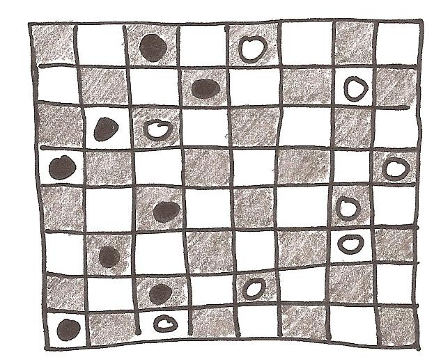
Figure 7.1: A position of Northcott’s Game

Clearly each row functions independently, so Northcott’s Game is really a sum of eight independent games. However, the standard partizan theory isn’t directly applicable, because this game is loopy, meaning that the players can return the board to a prior state if they so choose:

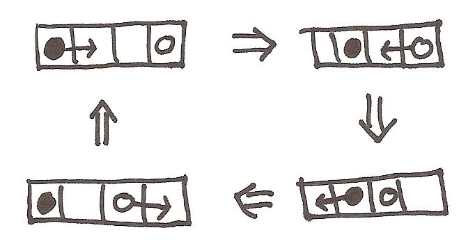
Figure 7.2: Loops can occur in Northcott’s Game.

Consequently, there is no guarantee that the game will ever come to an end, and draws are possible. We assume that each player prefers victory to a draw and a draw to defeat. Because of this extra possibility, it is conceivable that in some positions, neither player would have a winning strategy, but both players would have a strategy guaranteeing a drwa.

Suppose that we changed the rules, so that a player could only move his pieces forward, towards his opponent’s. Then the game would become loopfree, and in fact, it becomes nothing but Nim in disguise! Given a position of Northcott’s Game, one simply counts the number of empty squares between the two pieces in each row, and creates a Nim-heap of the same size:

Figure 7.3: Converting the position of Figure 7.1 into a Nim position.

The resulting Nim position is equivalent: taking $n$ counters from a Nim pile corresponds to moving your piece in the corresponding row $n$ squares forward. This works as long as we forbid backwards moves.

However, it turns out that this prohibition has no strategic effect. Whichever player has a winning strategy in the no-backwards-move variant can use the same strategy in the full game. If her opponent ever moves a piece backwards by $x$ squares, she moves her own piece forwards by $x$ squares, cancelling her opponent’s move. This strategy guarantees that the game actually ends, because the pieces of the player using the strategy are always moving forwards, which cannot go on indefinitely. So Northcott’s Game is still nothing but Nim in disguise. The moral of the story is that loopy games can sometimes be analyzed using partizan theory (Sprague-Grundy theory in this case).

We now consider two case studies of real-life games that can be partially analyzed using the standard partizan theory, even though they technically aren’t partizan games themselves.

7.2 Dots-and-Boxes

Unlike Northcott’s Game, Dots-and-Boxes (also known as Squares) is a game that people actually play. This is a pencil and paper game, played on a square grid of dots. Players take turns drawing line segments between orthogonally adjacent dots. Whenever you complete the fourth side of a box, you claim the box by writing your initials in it, and get another move. It is possible to chain together these extra moves, and take many boxes in a single turn:

Figure 7.4: Alice takes three boxes in one turn.

Eventually the board fills up, and the game ends. The player with the most boxes claimed wins. Victory is not decided by the normal play rule, making the standard theory of partizan games inapplicable.

Most people play Dots-and-Boxes by making random moves until all remaining moves create a three-sided box. Then the players take turn giving each other larger and larger chains.

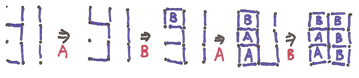
Figure 7.5: Alice gives Bob a box. Bob takes it and gives Alice two boxes. Alice takes them and gives Bob three boxes.

Oddly enough, there is a simple and little-known trick which easily beats the naïve strategy. When an opponent gives you three or more boxes, it is always possible to take all but two of them, and give two to your opponent. Your opponent takes the two boxes, and is then usually forced to give you another long chain of boxes.

For instance, in the following position,

the naïve strategy is to move to something like

which then gives your opponent more boxes than you obtained your self. The better move is the following:

From this position, your opponent might as well take the two boxes, but is then forced to give you the other long chain:

This trick is tied to a general phenomenon, of loony positions. Rather than giving a formal definition, we give an example.

Let $P_{1}$ be the following complicated position:

Surprisingly, we can show that this position is a win for the first player, without even exhibiting a specific strategy. To see this, let $P_{2}$ be the following position, in which Alice has the two squares in the bottom left corner:

Let $k$ be the final score for Alice if she moves first in $P_{2}$ and both players play optimally.

Since there are an odd number of boxes on the board, $k$ cannot be zero. Now break into cases according to the sign of $k$.

• If $k>0$, then the first player can win $P_{1}$ by taking the two boxes as well as the name “Alice.”

• If $k<0$, then the first player can win $P_{1}$ by naming her opponent “Alice” and declining the two boxes, as follows:

  

  Now “Alice” might as well take the two boxes, resulting in position $P_{2}$. Then because $k<0$, Alice’s opponent can guarantee a win. If “Alice” doesn’t take the two boxes, her opponent can just take them on her next turn, with no adverse effect.

So either way, the first player has a winning strategy in $P_{1}$. Actually applying this strategy is made difficult by the fact that we have to completely evaluate $P_{2}$ to tell which move to make in $P_{1}$.

In general, a loony position is one containing two adjacent boxes, such that

• There is no wall between the two boxes

• One of the two boxes has three walls around it.

• The other box has exactly two walls around it.

• The two boxes are not part of one of the following configurations:

  

The general fact about loony positions is that the first player is always able to win a weak majority of the remaining pieces on the board. This follows by essentially the same argument used to analyze the complicated position above. In the case where there are an odd number of boxes on the board, and neither player has already taken any boxes, it follows that a loony position is a win for the first player. Here are some examples of loony positions:

The red asterisks indicate why each position is loony. Here are some examples of non-loony positions:

It can be shown that whenever some squares are available to be taken, and the position is not loony, then you might as well take them.

A loony move is one that creates a loony position. Note that giving away a long chain (three or more boxes) or a loop is always a loony move. When giving away two boxes, it is always possible to do so in a non-loony way:

In the vast majority of Dots-and-Boxes games, somebody eventually gives a way a long chain. Usually, few boxes have been claimed when this first happens (or both players have claimed about the same amount, because they have been trading chains of length one and two), so the player who gives away the first long chain loses under perfect play.

Interestingly, the player who first makes a loony move can be predicted in terms of the parity of the number of long chains on the board. As the game proceeds towards its end, chains begin to form and the number of long chains begins to crystallize. Between experts, Dots-and-Boxes turns into a fight to control this number. For more information, I refer the interested reader to Elwyn Berlekamp’s The Dots and Boxes Game.

To connect Dots-and-Boxes to the standard theory of partizan games (in fact, to Sprague-Grundy theory), consider the variant game of Nimdots. This is played exactly the same as Dots-and-Boxes except that the player who makes the last move loses. A few comments are in order:

• Despite appearances to the contrary, Nimdots is actually played by the normal play rule, not the misère rule. The reason is that the normal rule precisely says that you lose when it’s your turn but you can’t move. In Nimdots, the player who makes the last move always completes a box. He then gets a bonus turn, which he is unable to complete, because the game is over!

• Who claims each box is completely irrelevant, since the final outcome isn’t decided by score. This makes Nimdots be impartial.

• As in Dots-and-Boxes, a loony move is generally bad. In fact, in Nimdots, a loony move is always a losing move, by the same arguments as above. In fact, since we are using the normal play rule, we might as well make loony moves illegal, and consider no loony positions.

• If you give away some boxes without making a non-loony move, your opponent might as well take them. But there is no score, so it doesn’t matter who takes the boxes, and we could simply have the boxes get magically eaten up after any move which gives away boxes.

With these rule modifications, there are no more entailed moves, and Nimdots becomes a bona fide impartial game, so we can apply Sprague-Grundy theory. For example, here is a table showing the Sprague-Grundy numbers of some small Nimdots positions (taken from page 559 of Winning Ways).

This sort of analysis is actually useful because positions in Nimdots and Dots-and-Boxes can often decompose as sums of smaller positions. And oddly enough, in some cases, a Nimdots positions replicate impartial games like Kayles (see chapter 16 of Winning Ways for examples).

The connection between Dots-and-Boxes and Nimdots comes by seeing Nimdots as an approximation to Dots-and-Boxes. In Dots-and-Boxes, the first player to make a loony move usually loses. in Nimdots, the first player to make a loony move always loses. So even though the winner is determined by completely different means in the two games, they tend to have similar outcomes, at least early in the game.

This gives an (imperfect and incomplete) “mathematical” strategy for Dots-and-Boxes: pretend that the position is a Nimdots position, and use this to make sure that your opponent ends up making the first loony move. In order for the loony-move fight to even be worthwhile, you also need to ensure that there are long enough chains. In the process of using this strategy, one might actually sacrifice some boxes to your opponent, for a better final score. For instance, in Figure 7.6, the only winning move is to prematurely sacrifice two boxes.

Figure 7.6: The only winning move is (a), which sacrifices two boxes. The alternative move at (b) sacrifices zero boxes, but ultimately loses.

The mathematical strategy is imperfect, so some people have advocated alternative strategies. On his now-defunct Geocities page, Ilan Vardi suggested a strategy based on

(a)

Making lots of shorter chains, and loops, which tend to decrease the value of winning the Nimdots fight.

(b)

“Nibbling,” allowing your opponent to win the Nimdots/loony-move fight, but at a cost.

(c)

“Pre-emptive sacrifices,” in which you make a loony-move in a long chain before the chain gets especially long. This breaks up chains early, helping to accomplish (a). Such moves can only work if you are already ahead score-wise, via (b).

As Ilan Vardi notes, there are some cases in Dots-and-Boxes in which the only winning move is loony:

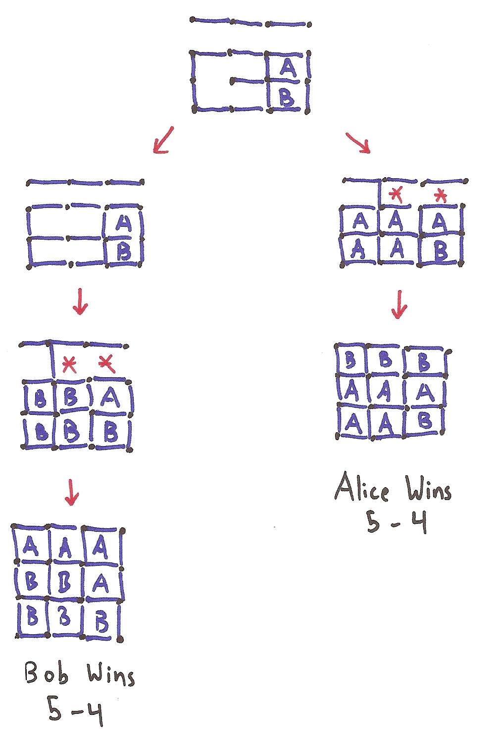
Figure 7.7: In the top position, with Alice to move, the move at the left is the only non-loony move. However, it ultimately loses, giving Bob most of the boxes. On the other hand, the move on the right is technically loony, but gives Alice the win, with 5 of the 9 boxes already.

According to Vardi, some of the analyses of specific positions in Berlekamp’s The Dots and Boxes Game are incorrect because of the false assumption that loony moves are always bad.

Unlike many of the games we have considered so far, there is little hope of giving a general analysis of Dots-and-Boxes, since determining the outcome of a Dots-and-Boxes position is NP-hard, as shown by Elwyn Berlekamp in the last chapter of his book.

7.3 Go

Go (also known as Baduk and Weiqi) is an ancient boardgame that is popular in China, Japan, the United States, and New Zealand, among other places. It is frequently considered to have the most strategic depth of any boardgame commonly played, more than Chess.

In Go, two players, Black and White, alternatively place stones on a $19\times 19$ board. Unlike Chess or Checkers, pieces are played on the corners of the squares, as in Figure 7.8. A group of stones is a set of stones of one color that is connected (by means of direct orthogonal connections). So in the following position, Black has 4 groups and White has 1 group:

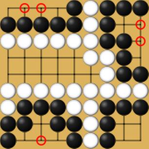
Figure 7.8: Image taken from the Wikipedia article Life and Death on June 6, 2011.

The liberties of a group are the number of empty squares. Once a group has no liberties, its pieces are captured and removed from the board, and given to the opposing player. There are some additional prohibitions against suicidal moves and moves which exactly reverse the previous move or return the board to a prior state. Some of these rules vary between different rulesets.

Players are also allowed to pass, and the game ends when both players pass. The rules for scoring are actually very complicated and vary by ruleset, but roughly speaking you get a point for each captured opponent stone, and a point for each empty space that is surrounded by pieces of your own color.

In the following position, if there were no stones captured, then Black would win by four points:

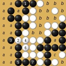
Figure 7.9: Black has 17 points of territory (the a’s) and White has 13 (the b’s). Image taken from the Wikipedia article Rules of Go on June 6, 2011.

(The scoring rule mentioned above is the one used in Japan and the United States. In China, you also get points for your own pieces on the board, but not for prisoners, which tends to make the final score difference almost identical to the result of Japanese scoring.)

There is a great deal of terminology and literature related to this game, so we can barely scratch the surface. One thing worth pointing out is that it is sometimes possible for a group of stones to be indestructible. This is called life. Here is an example:

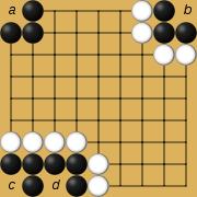
Figure 7.10: The black group in the bottom left corner has two eyes, so it is alive. There is no way for White to capture it, since White would need to move in positions $c$ and $d$ simultaneously. The other black groups do not have two eyes, and could be taken. For example, if White moves at $b$, the top right black group would be captured. (Image taken from the Wikipedia article Life and Death on June 6, 2011.)

This example shows the general principle that two “eyes” ensures life.

Another strategic concept is seki, which refers to positions in which neither player wants to move, like the following:

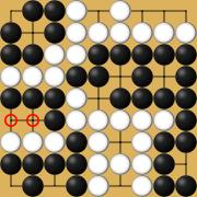
Figure 7.11: If either player moves in one of the red circled positions, his opponent will move in the other and take one of his groups. So neither player will play in those positions, and they will remain empty. (Image taken from the Wikipedia article Go (game) on June 6, 2011.)

Because neither player has an obligation to move, both players will simply ignore this area until the end of the game, and the spaces in this position will count towards neither player.

Like Dots-and-Boxes, Go is not played by the normal play rule, but uses scores instead. However, there is a naïve way to turn a Go position into a partizan game position that actually works fairly well, and is employed by Berlekamp and Wolfe in their book Mathematical Go: Chilling Gets the Last Point. Basically, each final position in which no moves remain is replaced by its score, interpreted as a surreal number.

For instance, we have

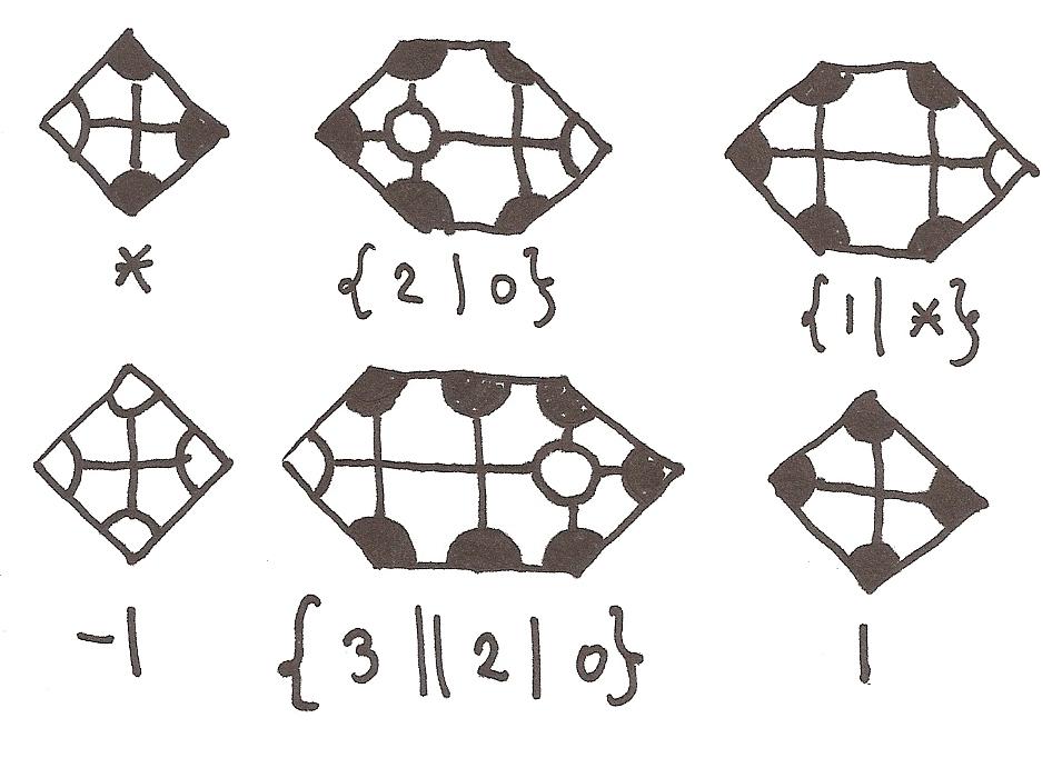
Figure 7.12: Small positions in Go, taken from Berlekamp and Wolfe. The pieces along the boundary are assumed to be alive.

This approach works because of number avoidance. Converting Go endgames into surreal numbers adds extra options, but we can assume that the players never use these extra options, because of number avoidance. For this to work, we need the fact that a non-endgame Go position isn’t a number. Unfortunately, some are, like the following:

However, something slightly stronger than number-avoidance is actually true:

Theorem 7.3.1.

Let $A,B,C,\ldots,D,E,F,\ldots$ be short partizan games, such that

$$\max(R(A),R(B),\ldots)\geq\min(L(D),L(E),\ldots),$$

and let $x$ be a number. Then

$$\{A,B,C,\ldots|D,E,F,\ldots\}+x=\{A+x,B+x,\ldots|D+x,E+x,\ldots\}.$$

Proof.

If $\{A,B,C,\ldots|D,E,F,\ldots\}$ is not a number, then this follows by number avoidance. It also follows by number avoidance if $\{A+x,B+x,\ldots|D+x,E+X,\ldots\}$ is not a number. Otherwise, there is some number $y$, equal to $\{A,B,\ldots|D,E,\ldots\}$ such that $A,B,C,\ldots\lhd y\lhd D,E,F,\ldots$. But by definition of $L(\cdot)$ and $R(\cdot)$, it follows that

$$\max(R(A),R(B),\ldots)\leq y\leq\min(L(D),L(E),\ldots),$$

since it is a general fact that $y\lhd G$ implies that $y\leq L(G)$ and similarly $G\lhd y\Rightarrow R(G)\leq y$. So it must be the case that $\max(R(A),R(B),\ldots)=y=\min(L(A),L(B),\ldots)$. Thus

$$\{A,B,C,\ldots|D,E,F,\ldots\}=\max(R(A),R(B),\ldots).$$

By the same token,

$$\{A+x,B+x,\ldots|D+x,E+x,\ldots\}=\max(R(A+x),R(B+x),\ldots)$$

$$=\max(R(A)+x,R(B)+x,\ldots)=\{A,B,\ldots|D,E,\ldots\}+x.$$

∎

Now Go positions always have the property that $\max_{G^{L}}(R(G^{L}))\geq\min_{G^{R}}(L(G^{R}))$, because players are not under compulsion to pass. There is no way to create a position like $\{0|4\}$ in Go (which would asymmetrically be given the value $1$ by our translation), because in such a position, neither player wants to move, and the position will be a seki endgame position that should have been directly turned into a number.

Interestingly enough, many simple Go positions end up taking values that are Even or Odd, in the sense of Section 6.1. This comes about because we can assign a parity to each Go position, counting the number of prisoners and emtpy spaces on the board, and the parity is reversed after each move. And an endgame will have an odd score iff its positional parity is odd (unless there are dame).

Then because most of the values that arise are even and odd, we can describe them as Norton multiples of $1*$. Replacing the position $X.(1*)$ with $X$ creates a simpler description of the same position. This operation is the “chilling” operation referenced in the title of Wolfe and Berlekamp’s books. It is an instance of the cooling operation of “thermography,” which is closely related to the mean value theory.

A lot of research has gone into studying ko situations like the following:

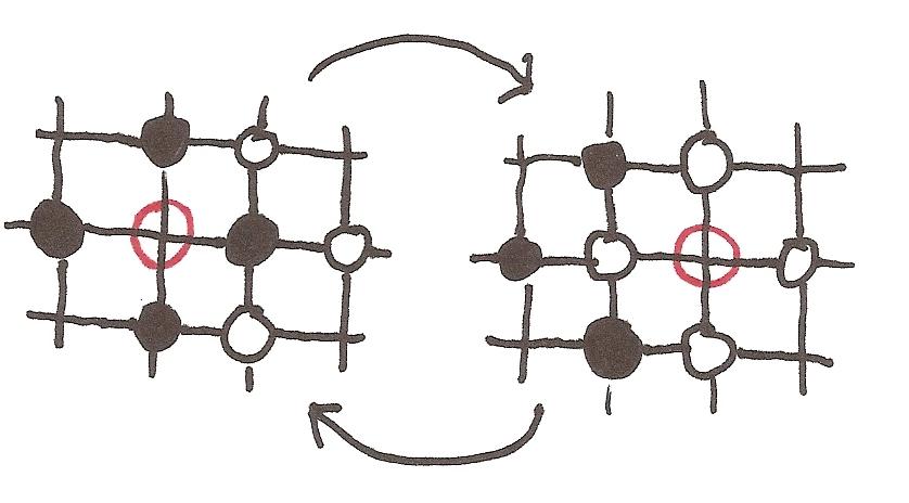
Figure 7.13: From the position on the left, White can move to the position on the right by playing in the circled position. But from the position on the right, Black can move directly back to the position on the right, by playing in the circled position.

The rules of Go include a proviso that forbids directly undoing a previous move. However, nothing prevents White from making a threat somewhere else, which Black must respond to - and then after Black responds elsewhere, White can move back in the ko. This can go back and forth several rounds, in what is known as a kofight. While some players of Go see kofights as mere randomness (a player once told me it was like shooting craps), many combinatorial game theorists have mathematically examined ko positions, using extensions of mean value theory and “thermography” for loopy games.

7.4 Changing the theory

In some cases, we need a different theory from the standard one discussed so far. The examples in this section are not games people play, but show how alternative theories can arise in constructed games.

Consider first the following game, One of the King’s Horses: a number of chess knights sit on a square board, and players take turns moving them towards the top left corner. The pieces move like knights in chess, except only in the four northwestern directions:

Each turn, you move one piece, but multiple pieces are allowed to occupy the same square. You lose when you cannot move.

Clearly, this is an impartial game with the normal play rule, and each piece is moving completely independently of all the others, so the game decomposes as a sum. Consequently we can “solve” the game by figuring out the Sprague-Grundy value of each position on the board. Here is a table showing the values in the top left corner of the board:

0	0	1	1	0	0	1	1	0	0	1	1	0	0	1	1
0	0	2	1	0	0	1	1	0	0	1	1	0	0	1	1
1	2	2	2	③	2	2	2	3	2	2	2	3	2	2	2
1	1	2	1	4	③	2	3	3	3	2	3	3	3	2	3
0	0	3	④	0	0	1	1	0	0	1	1	0	0	1	1
0	0	②	③	0	0	2	1	0	0	1	1	0	0	1	1
1	1	2	2	1	2	2	2	3	2	2	2	3	2	2	2
1	1	2	3	1	1	2	1	4	3	2	3	3	3	2	3
0	0	3	3	0	0	3	4	0	0	1	1	0	0	1	1
0	0	2	3	0	0	2	3	0	0	2	1	0	0	1	1
1	1	2	2	1	1	2	2	1	2	2	2	3	2	2	2
1	1	2	3	1	1	2	3	1	1	2	1	4	3	2	3
0	0	3	3	0	0	3	3	0	0	3	4	0	0	1	1
0	0	2	3	0	0	2	3	0	0	2	3	0	0	2	1
1	1	2	2	1	1	2	2	1	1	2	2	1	2	2	2
1	1	2	3	1	1	2	3	1	1	2	3	1	1	2	1

So for instance, if there are pieces on the circled positions, the combined value is

$$3+_{2}3+_{2}2+_{2}3+_{2}4=5$$

Since $5\neq 0$, this position is a first-player win. The table shown above has a fairly simple and repetitive pattern, which gives the general strategy for One of the King’s Horses.

Now consider the variant All of the King’s Horses, in which you move every piece on your turn, rather than selecting one. Note that once one of the pieces reaches the top left corner of the board, the game is over, since you are required to move all the pieces on your turn, and this becomes impossible once one of the pieces reaches the home corner.

This game no longer corresponds to a sum, but instead to what Winning Ways calls a join. Whereas a sum is recursively defined as

$$G+H=\{G^{L}+H,G+H^{L}|G^{R}+H,G+H^{R}\},$$

a join is defined recursively as

$$G\wedge H=\{G^{L}\wedge H^{L}|G^{R}\wedge H^{R}\},$$

where $G^{*}$ and $H^{*}$ range over the options of $G$ and $H$. In a join of two games, you must move in both components on each turn.

Just as sums of impartial games are governed by Sprague-Grundy numbers, joins of impartial games are governed by remoteness. If $G$ is an impartial game, its remoteness $r(G)$ is defined recursively as follows:

• If $G$ has no options, then $r(G)$ is zero.

• If some option of $G$ has even remoteness, then $r(G)$ is one more than the minimum $r(G^{\prime})$ where $G^{\prime}$ ranges over options of $G$ such that $r(G^{\prime})$ is even.

• Otherwise, $r(G)$ is one more than the maximum $r(G^{\prime})$ for $G^{\prime}$ an option of $r(G)$.

Note that $r(G)$ is odd if and only if some option of $G$ has even remoteness. Consequently, a game is a second-player win if its remoteness number is even, and a first-player win otherwise. The remoteness of a Nim heap with $n$ counters is $0$ if $n=0$, and $1$ otherwise, since every Nim-heap after the zeroth one has the zeroth one as an option.

The remoteness is roughly a measure of how quickly the winning player can bring the game to an end, assuming that the losing player is trying to draw out the game as long as possible.

Remoteness governs the outcome of joins of impartial games in the same way that Sprague-Grundy numbers govern the outcome of sums:

Theorem 7.4.1.

If $G_{1},\ldots,G_{n}$ are impartial games, then the join $G_{1}\wedge\cdots\wedge G_{n}$ is a second-player win if $\min(r(G_{1}),\ldots,r(G_{n}))$ is even, and a first-player win otherwise.

Proof.

First of all note that if $G$ is any nonzero impartial game, then $r(G)=r(G^{\prime})-1$ for some option $G^{\prime}$ of $G$. Also, if $r(G)$ is odd then some option of $G$ has even remoteness.

To prove the theorem, first consider the case where one of the $G_{i}$ has no options, so $r(G_{i})=0$. Then neither does the $G_{1}\wedge\cdots\wedge G_{n}$. A game with no options is a second-player win (because whoever goes first immediately loses). And as expected, and $\min(r(G_{1}),\ldots,r(G_{n}))=0$ which is even.

Now suppose that every $G_{i}$ has an option. First consider the case where $\min(r(G_{1}),\ldots,r(G_{n}))$ is odd. Then for every $i$ we can find an option $G_{i}^{\prime}$ of $G_{i}$, such that $r(G_{i})=r(G_{i}^{\prime})+1$. In particular then,

$$\min(r(G_{1}^{\prime}),\ldots,r(G_{n}^{\prime}))=\min(r(G_{1}),\ldots,r(G_{n}))\text{ is even,},$$

so by induction $G_{1}^{\prime}\wedge\cdots\wedge G_{n}^{\prime}$ is a second-player win. Therefore $G_{1}\wedge\cdots\wedge G_{n}$ is a first-player win, as desired.

On the other hand, suppose that $\min(r(G_{1}),\ldots,r(G_{n}))$ is even. Let $r(G_{i})=\min(r(G_{1}),\ldots,r(G_{n}))$. Suppose for the sake of contradiction that there is some option $G_{1}^{\prime}\wedge\cdots\wedge G_{n}^{\prime}$ of $G_{1}\wedge\cdots\wedge G_{n}$ such that $\min(r(G_{1}^{\prime}),\ldots,r(G_{n}^{\prime}))$ is also even. Let $r(G_{j}^{\prime})=\min(r(G_{1}^{\prime}),\ldots,r(G_{n}^{\prime}))$. Since $r(G_{j}^{\prime})$ is even, it follows that $r(G_{j})$ is odd and at most $r(G_{j}^{\prime})+1$. Then

$$r(G_{i})=\min(r(G_{1}),\ldots,r(G_{n}))\leq r(G_{j})\leq r(G_{j}^{\prime})+1,$$ (7.1)

On the other hand, since $r(G_{i})$ is even, every option of $G_{i}$ has odd remoteness, and in particular $r(G_{i}^{\prime})$ is odd and at most $r(G_{i})-1$. Then

$$r(G_{j}^{\prime})=\min(r(G_{1}^{\prime}),\ldots,r(G_{n}^{\prime}))\leq r(G_{i}^{\prime})\leq r(G_{i})-1.$$

Combining with (7.1), it follows that $r(G_{j}^{\prime})=r(G_{i})-1$, contradicting the fact that $r(G_{i})$ and $r(G_{j}^{\prime})$ are both even. ∎

In fact, from this we can determine the remoteness of a join of two games:

Corollary 7.4.2.

Let $G$ and $H$ be impartial games. Then $r(G\wedge H)=\min(r(G),r(H))$.

Proof.

Let $a_{0}=\{|\}$, and $a_{n}=\{a_{n-1}|a_{n-1}\}$ for $n>0$. Then $r(a_{n})=n$. Now if $K$ is any impartial game, then $r(K)$ is uniquely determined by the outcomes of $K\wedge a_{n}$ for every $n$. To see this, suppose that $K_{1}$ and $K_{2}$ have differing remotenesses, specifically $n=r(K_{1})<r(K_{2})$. Then $\min(r(K_{1}),r(a_{n+1}))=\min(n,n+1)=n$, while $r(K_{2})\geq n+1$, so that $\min(r(K_{2}),r(a_{n+1}))=n+1$. Since $n$ and $n+1$ have different parities, it follows by the theorem that $K_{1}\wedge a_{n+1}$ and $K_{2}\wedge a_{n+1}$ have different outcomes.

Now let $G$ and $H$ be impartial games, and let $n=\min(r(G),r(H))$. Then for every $k$,

$$\min(r(G),r(H),r(a_{k}))=\min(r(a_{n}),r(a_{k})),$$

so that $G\wedge H\wedge a_{k}$ has the same outcome as $a_{n}\wedge a_{k}$ for all $k$. But then since $G\wedge H\wedge a_{k}=(G\wedge H)\wedge a_{k}$, it follows by the previous paragraph that $(G\wedge H)$ and $a_{n}$ must have the same remoteness. But since the remoteness of $a_{n}$ is $n$, $r(G\wedge H)$ must also be $n=\min(r(G),r(H))$. ∎

Using these rules, we can evaluate a position of All the King’s Horses using the following table showing the remoteness of each location:

0	0	1	1	2	2	3	3	4	4	5	5	6	6	7	7
0	0	1	1	2	2	3	3	4	4	5	5	6	6	7	7
1	1	1	1	③	3	3	3	5	5	5	5	7	7	7	7
1	1	1	3	3	③	3	5	5	5	5	7	7	7	7	9
2	②	3	3	4	4	5	5	⑥	6	7	7	8	8	9	9
2	2	3	3	4	4	5	5	6	6	7	7	8	8	9	9
3	3	3	3	5	5	5	5	7	7	7	7	9	9	9	9
3	3	3	5	5	5	5	7	7	7	7	9	9	9	9	11
4	4	5	5	6	6	7	7	8	8	9	9	10	10	11	11
4	4	5	5	6	6	7	7	8	8	9	9	10	10	11	11
5	5	5	5	7	7	7	7	9	9	9	9	11	11	11	11
5	5	5	7	7	7	7	9	9	9	9	11	11	11	11	13
6	6	7	7	8	8	9	9	10	10	11	11	12	12	13	13
6	6	7	7	8	8	9	9	10	10	11	11	12	12	13	13
7	7	7	7	9	9	9	9	11	11	11	11	13	13	13	13
7	7	7	9	9	9	9	11	11	11	11	13	13	13	13	15

So for instance, if there are pieces on the circled positions, then the combined remoteness is

$$\min(3,3,2,6)=2,$$

and $2$ is even, so the combined position is a win for the second-player.

The full partizan theory of joins isn’t much more complicated than the impartial theory, because of the fact that play necessarily alternates in each component (unlike in the theory of sums, where a player might make two moves in a component without an intervening move by the opponent).

A third operation, analogous to sums and joins, is the union, defined recursively as

$$G\vee H=\{G^{L}\vee H,G^{L}\vee H^{L},G\vee H^{L}|G^{R}\vee H,G^{R}\vee H^{R},G\vee H^{R}\}$$

In a union of two games, you can move in one or both components. More generally, in a union of $n$ games, you can on your turn move in any (nonempty) set of components. The corresponding variant of All the King’s Horses is Some of the King’s Horses, in which you can move any positive number of the horses, on each turn.

For impartial games, the theory of unions turns out to be trivial: a union of two games is a second-player win if and only if both are second-player wins themselves. If $G$ and $H$ are both second-player wins, then any move in $G$, $H$, or both, will result in at least one of $G$ and $H$ being replaced with a first-player win - and by induction such a union is itself a first player win. On the other hand, if at least one of $G$ and $H$ is a first-player win, then the first player to move in $G\vee H$ can just move in whichever components are not second-player wins, creating a position whose every component is a second-player win.

So to analyze Some of the King’s Horses, we only need to mark whether each position is a first-player win or a second-player win:

2	2	1	1	2	2	1	1
2	2	1	1	2	2	1	1
1	1	1	1	1	1	1	1
1	1	1	1	1	1	1	1
2	2	1	1	2	2	1	1
2	2	1	1	2	2	1	1
1	1	1	1	1	1	1	1
1	1	1	1	1	1	1	1

7.5 Highlights from Winning Ways Part 2

The entire second volume of Winning Ways is an exposition of alternate theories to the standard partizan theory.

7.5.1 Unions of partizan games

In the partizan case, unions are much more interesting. Without proofs, here is a summary of what happens, taken from Chapter 10 of Winning Ways:

• To each game, we associate an expression of the form $x_{n}y_{m}$ where $x$ and $y$ are dyadic rationals and $n$ and $m$ are nonnegative integers. The $x_{n}$ part is the “left tally” consisting of a “toll” of $x$ and a “timer” $n$, and similarly $y_{m}$ is the “right tally.” The expression $x$ is short for $x_{0}x_{0}$.

• These expressions are added as follows:

  $$x_{n}y_{m}+w_{i}z_{j}=(x+w)_{\max(n,i)}(y+z)_{\max(m,j)}.$$

• In a position with value $x_{n}y_{m}$, if Left goes first then she wins iff $x>0$ or $x=0$ and $n$ is odd. If Right goes first then he wins iff $y<0$ or $y=0$ and $m$ is odd.

Given a game $G=\{G^{L}|G^{R}\}$, the tallies can be found by the following complicated procedure, copied verbatim out of page 308 of Winning Ways:

To find the tallies from options:

Shortlist all the $G^{L}$ with the GREATEST RIGHT toll, and all the $G^{R}$ with the LEAST LEFT toll. Then on each side select the tally with the LARGEST EVEN timer if there is one, and otherwise the LEAST ODD timer, obtaining the form

$$G=\{\ldots x_{a}|y_{b}\ldots\}.$$

• If $x>y$ (HOT), the tallies are $x_{a+1}y_{b+1}$.

• If $x<y$ (COLD), $G$ is the simplest number between $x$ and $y$, including $x$ as a possibility just if $a$ is odd, $y$ just if $b$ is odd.

• If $x=y$ (TEPID), try $x_{a+1}y_{b+1}$. But if just one of $a+1$ and $b+1$ is an even number, increase the other (if necessary) by just enough to make it a larger odd number. If both are even, replace each of them by 0.

Here they are identifying a number $z$ with tallies $z_{0}z_{0}$. If I understand Winning Ways correctly, the cases where there are no left options or no right options fall under the COLD case.

7.5.2 Loopy games

Another part of Winning Ways Volume 2 considers loopy games, which have no guarantee of ever ending. The situation where play continues indefinitely are draws, are ties by default. However, we actually allow games to specify the winner of every infinite sequence of plays. Given a game $\gamma$, the variants $\gamma^{+}$ and $\gamma^{-}$ are the games formed by resolving all ties in favor of Left and Right, respectively.

Sums of infinite games are defined in the usual way, though to specify the winner, the following rules are used:

• If the sum of the games comes to an end, the winner is decided by the normal rule, as usual.

• Otherwise, if Left or Right wins every component in which play never came to an end, then Left or Right wins the sum.

• Otherwise the game is a tie.

Given sums, we define equivalence by $G=H$ if $G+K$ and $H+K$ have the same outcome under perfect play for every loopy game $K$.

A stopper is a game which is guaranteed to end when played in isolation, because it has no infinite alternating sequences of play, like

$$G\to G^{L}\to G^{LR}\to G^{LRL}\to G^{LRLR}\to\cdots$$

Finite stoppers have canonical forms in the same way that loopfree partizan games do.

For most (but not all) loopy games $\gamma$, there exist stoppers $s$ and $t$ such that

$$\gamma^{+}=s^{+}\text{ and }\gamma^{-}=t^{-}.$$

These games are called the onside and offside of $\gamma$ respectively, and we write $\gamma=s\&t$ to indicate this relationship. These stoppers can be found by the operation of “sidling” described on pages 338-342 of Winning Ways. It is always the case that $s\geq t$. When $\gamma$ is already a stopper, $s$ and $t$ can be taken to be $\gamma$.

Given two games $s\&t$ and $x\&y$, the sum $(s\&t)+(x\&y)$ is $u\&v$ where $u$ is the upsum of $s$ and $x$, while $v$ is the downsum of $t$ and $y$. The upsum of two games is the onside of their sum, and the downsum is the offside of their sum.

7.5.3 Misère games

Winning ways Chapter 13 “Survival in the Lost World” and On Numbers and Games Chapter 12 “How to Lose when you Must” both consider the theory of impartial misère games. These are exactly like normal impartial games, except that we play by a different rule, the misère rule in which the last player able to move loses. The theory turns out to be far more complicated and lest satisfactory than the Sprague-Grundy theory for normal impartial games. For games $G$ and $H$, Conway says that $G$ is like $H$ if $G+K$ and $H+K$ have the same misère outcome for all $K$, and then goes on to show that every game $G$ has a canonical simplest form, modulo this relation. However, the reductions allowed are not very effective, in the sense that the number of misère impartial games born on day $n$ grows astronomically, like the sequence

$$\left\lceil\gamma_{0}\right\rceil,\left\lceil 2^{\gamma_{0}}\right\rceil,\left\lceil 2^{2^{\gamma_{0}}}\right\rceil,\left\lceil 2^{2^{2^{\gamma_{0}}}}\right\rceil,\ldots$$

for $\gamma_{0}\approx 0.149027$ (see page 152 of ONAG). Conway is able to give more complete analyses of certain “tame” games which behave similar to mis‘ere Nim positions, and Winning Ways contains additional comments about games that are almost tame but in general, the theory is very spotty. For example, these results do not provide a complete analysis of Misère Kayles.

7.6 Misère Indistinguishability Quotients

However, a solution of Misère Kayles was obtained through other means by William Sibert. Sibert found a complete description of the Kayles positions for which misère outcome differs from normal outcome. His solution can be found on page 446-451 of Winning Ways.

Let $\mathcal{K}$ be the set of all Kayles positions. We say that $G$ and $H\in\mathcal{K}$ are indistinguishable if $G+X$ and $H+X$ have the same misère outcome for every $X$ in $\mathcal{K}$. If we let $X$ range over all impartial games, this would be the same as Conway’s relation $G$ “is like” $H$. By limiting $X$ to range over only positions that occur in Kayles, the equivalence relation becomes coarser, and the quotient space becomes smaller. In fact, using Sibert’s solution, one can show that the quotient space has size 48. An alternate way of describing Sibert’s solution is to give a description of this monoid, a table showing which equivalence classes have which outcomes, and a table showing which element of the monoid corresponds to a Kayles row of each possible length.

This sort of analysis has been extended to many other misère games by Plambeck, Siegel, and others. For a given class of misère games, let $\mathcal{G}$ be the closure of this class under addition. Then for $X,Y\in\mathcal{G}$, we say that $X$ and $Y$ are indistinguishable if $X+Z$ and $Y+Z$ have the same misère outcome for all $z\in\mathcal{G}$. We then let the indistinguishability quotient be $\mathcal{G}$ modulo indistinguishability. The point of this construction is that

• The indistinguishablity quotient is a monoid, and there is a natural surjective monoid homomorphism (the “pretending function”) from $\mathcal{G}$ (as a monoid with addition) to the indistinguishability quotient.

• There is a map from the indistinguishability quotient to the set of outcomes, whose composition with the pretending function yields the map from games to their outcomes.

Using these two maps, we can then analyze any sum of games in $\mathcal{G}$, assuming the structure of the indistinguishability quotient is manageable.

For many cases, like Kayles, the indistinguishability quotient is finite. In fact Aaron Siegel has written software to calculate the indistinguishability quotient when it is finite, for a large class of games. This seems to be the best way to solve or analyze misère games so far.

7.7 Indistinguishability in General

The general setup of (additive) combinatorial game theory could be described as follows: we have a collection of games, each of which has an outcome. Additionally, we have various operations - ways of combining games. We want to characterize each game with a simpler object, a value, satisfying two conditions. First of all, the outcome of a game must be determined by the value, and second, the value of a combination of games must be determined by the values of the games being combined. The the value of a game contains all the information about the game that we care about, and two games having the same value can be considered equivalent.

Our goal is to make the set of values as simple and small as possible. We first throw out values that correspond to no games, making the map from games to values a surjection. Then the set of values becomes the quotient space of games modulo equivalence. This quotient space will be smallest when the equivalence relation is coarsest.

However, there are two requirements on the equivalence relation. First of all, it needs to respect outcomes: if two games are equivalent, then they must have the same outcome. And second, it must be compatible with the operations on games, so that the operations are well-defined on the quotient space.

Indistinguishability is the uniqe coarsest equivalence relation satisfying these properties, and the indistinguishability quotient of games modulo indistinguishability is thus the smallest set of values that are usable. It thus provides a canonical and optimal solution to the construction of the set of “values.”

The basic idea of indistinguishability is that two games should be indistinguishable if they are fully interchangeable, meaning that they can be exchanged in any context within a larger combination of games, without changing the outcome of the entire combination. For example if $G$ and $H$ are two indistinguishable partizan games, then

• $G$ and $H$ must have the same outcome.

• $23+G+\downarrow$ and $23+H+\downarrow$ must have the same outcome.

• $\{17*|G,6-G\}$ and $\{17*|H,6-H\}$ must have the same outcome

• And so on…

Conversely, if $G$ and $H$ are not indistinguishable, then there must be some context in which they cannot be interchanged.

The notion of indistinguishability is a relative one, that depends on the class of games being considered, the map from games to outcomes, and the set of operations being considered. Restricting the class of games makes indistinguishability coarser, which is how misère indistinguishability quotients are able to solve games like Misère Kayles, even when we cannot classify positions of Misère Kayles up to indistinguishability in the broader context of all misère impartial games.

Similarly, adding new operations into the mix makes indistinguishability finer. In the case of partizan games, by a lucky coincidence indistinguishability for the operation of addition alone is already compatible with negation and game-construction, so adding in these other two operations does not change indistinguishability. In other contexts this might not always work.

While never defined formally, the notion of indistinguishability is implicit in every chapter of the second volume of Winning Ways. For example, one can show that if our class of games is partizan games and our operation is unions, then two games $G$ and $H$ are indistinguishable if and only if they have the same tally. Similarly, if we are working with impartial games and joins, then two games $G$ and $H$ are indistinguishable if and only if they have the same remoteness (this follows by Theorem 7.7.3 below and what was shown in the first paragraph of the proof of Corollary 7.4.2 above). For misère impartial games, our indistinguishability agrees with the usual definition used by Siegel and Plambeck, because of Theorem 7.7.3 below. And for the standard theory of sums of partizan games, indistinguishability will just be the standard notion of equality that we have used so far.

To formally define indistinguishability, we need some notation. Let $S$ be a set of “games,” $O$ a set of “outcomes,” and $\operatorname{o^{\#}}:S\to O$ a map which assigns an outcome to each game. Let $f_{1},\ldots,f_{k}$ be “operations” $f_{i}:S^{n_{i}}\to S$ on the set of games.

Theorem 7.7.1.

There is a unique largest equivalence relation $\sim$ on $S$ having the following properties:

(a)

If $x\sim y$ then $\operatorname{o^{\#}}(x)=\operatorname{o^{\#}}(y)$.

(b)

If $1\leq i\leq k$, and if $x_{1},\ldots,x_{n_{i}},y_{1},\ldots,y_{n_{i}}$ are games in $S$ for which $x_{j}\sim y_{j}$ for every $1\leq j\leq n_{i}$, then $f_{i}(x_{1},\ldots,x_{n_{i}})\sim f_{i}(y_{1},\ldots,y_{n_{i}})$.

So if we have just one operation, say $\oplus$, then $\sim$ is the largest equivalence relation such that

$$x_{1}\sim y_{1}\text{ and }x_{2}\sim y_{2}\implies x_{1}\oplus x_{2}\sim y_{1}\oplus y_{2},$$

and such that $x\sim y$ implies that $x$ and $y$ have the same outcome. These conditions are equivalent to the claim that $\oplus$ and $\operatorname{o^{\#}}(\cdot)$ are well-defined on the quotient space of $\sim$.

Proof.

For notational simplicity, we assume that there is only one $f$, and that its arity is 2: $f:S^{2}\to S$. The proof works the same for more general situations.

Note that as long as $\sim$ is an equivalence relation, (b) is logically equivalent to the following assumptions

(c1)

If $x\sim x^{\prime}$, then $f(x,y)\sim f(x^{\prime},y)$.

(c2)

If $y\sim y^{\prime}$, then $f(x,y)\sim f(x,y^{\prime})$.

For if (b) is satisfied, then (c1) and (c2) both follow by reflexitivity of $\sim$. On the other hand, given (c1) and (c2), $x_{1}\sim y_{1}$ and $x_{2}\sim y_{2}$ imply that

$$f(x_{1},y_{1})\sim f(x_{2},y_{1})\sim f(x_{2},y_{2}),$$

using (c1) and (c2) for the first and second $\sim$, so that by transitivity $f(x_{1},y_{1})\sim f(x_{2},y_{2})$. These proofs easily generalize to the case where there is more than one $f$ or higher arities, though we need to replace (c1) and (c2) with $n_{1}+n_{2}+\cdots+n_{k}$ separate conditions, one for each parameter of each function.

We show that there is a unique largest relation satisfying (a), (c1) and (c2), and that it is an equivalence relation. This clearly implies our desired result.

Let $\mathcal{T}$ be the class of all relations $R$ satisfying

(A)

If $\operatorname{o^{\#}}(x)\neq\operatorname{o^{\#}}(y)$, then $x~{}R~{}y$.

(C1)

If $f(x,a)~{}R~{}f(y,a)$, then $x~{}R~{}y$.

(C2)

If $f(a,x)~{}R~{}f(a,y)$, then $x~{}R~{}y$.

It’s clear that $R$ satisfies (A), (C1), and (C2) if an only if the complement of $R$ satisfies (a), (c1), and (c2). Moreover, there is a unique smallest element $\not\sim$ of $\mathcal{T}$, the intersection of all relations in $\mathcal{T}$, and its complement is the unique largest relation satisfying (a), (c1), and (c2). We need to show that the complement $\sim$ of this minimal relation $\not\sim$ is an equivalence relation.

First of all, the relation $\neq$ also satisfies (A), (C1), (C2). By minimality of $\not\sim$, it follows that $x\not\sim y\implies x\neq y$, i.e., $x=y\implies x\sim y$. So $\sim$ is reflexive.

Second of all, if $R$ is any relation in $\mathcal{T}$, then the transpose relation $R^{\prime}$ given by $x~{}R^{\prime}~{}y\iff y~{}R~{}x$ also satisfies (A), (C1), and (C2). Thus $\not\sim$ must lie inside its transpose: $x\not\sim y\implies y\not\sim x$, and therefore $\sim$ is symmetric.

Finally, to see that $\not\sim$ is transitive, let $R$ be the relation given by

$$x~{}R~{}z\iff\forall y\in S:~{}x\not\sim y\vee y\not\sim z$$

where $\vee$ here means logical “or.” I claim that $R\in\mathcal{T}$. Indeed

$$\operatorname{o^{\#}}(x)\neq\operatorname{o^{\#}}(z)\implies\forall y\in S:~{}\operatorname{o^{\#}}(x)\neq\operatorname{o^{\#}}(y)\vee\operatorname{o^{\#}}(y)\neq\operatorname{o^{\#}}(z)$$

$$\implies\forall y\in S:~{}x\not\sim y\vee y\not\sim z\implies x~{}R~{}z$$

so (A) is satisfied. Similarly, for (C1):

$$f(x,a)~{}R~{}f(z,a)\implies\forall y\in S:~{}f(x,a)\not\sim y\vee y\not\sim f(z,a)$$

$$\implies\forall y\in S:~{}f(x,a)\not\sim f(y,a)\vee f(y,a)\not\sim f(z,a)\implies$$

$$\forall y\in S:~{}x\not\sim y\vee y\not\sim z\implies x~{}R~{}z,$$

using the fact that $\not\sim$ satisfies (C1). A similar argument shows that $R$ satisfies (C2). Then by minimality of $\not\sim$, we see that $x\not\sim y\implies x~{}R~{}y$, i.e.,

$$x\not\sim z\implies\forall y\in S:~{}x\not\sim y\vee y\not\sim z$$

which simply means that $\sim$ is transitive. ∎

Definition 7.7.2.

Given a class of games and a list of operations on games, we define indistinguishability (with respect to the given operations) to be the equivalence relation from the previous theorem, and denote it as $\approx_{f_{1},f_{2},\ldots,f_{k}}$. The quotient space of $S$ is the indistinguishability quotient.

In the case where there is a single binary operation, turning the class of games into a commutative monoid, indistinguishability has a simple definition:

Theorem 7.7.3.

Suppose that $\otimes:G\times G\to G$ is commutative and associative and has an identity $e$. Then $G,H\in S$ are indistinguishable (with respect to $\otimes$) if and only if $\operatorname{o^{\#}}(G\otimes X)=\operatorname{o^{\#}}(G\otimes X)$ for every $X\in S$.

Proof.

Let $\rho$ be the relation $G\,\rho\,H$ iff $\operatorname{o^{\#}}(G\otimes X)=\operatorname{o^{\#}}(H\otimes X)$ for every $X\in S$. I first claim that $\rho$ satisfies conditions (a) and (b) of Theorem 7.7.1. For (a), note that

$$G\,\rho\,H\Rightarrow\operatorname{o^{\#}}(G\otimes e)=\operatorname{o^{\#}}(H\otimes e).$$

But $G\otimes e=G$ and $H\otimes e=H$, so $G\,\rho\,H\Rightarrow\operatorname{o^{\#}}(G)=\operatorname{o^{\#}}(H)$. For (b), suppose that $G\,\rho\,G^{\prime}$ and $H\,\rho,H^{\prime}$. Then $G\otimes H\,\rho\,G^{\prime}\otimes H^{\prime}$, because for any $X\in S$,

$$\operatorname{o^{\#}}((G\otimes H)\otimes X)=\operatorname{o^{\#}}(G\otimes(H\otimes X))=\operatorname{o^{\#}}(G^{\prime}\otimes(H\otimes X))=$$

$$\operatorname{o^{\#}}(H\otimes(G^{\prime}\otimes X))=\operatorname{o^{\#}}(H^{\prime}\otimes(G^{\prime}\otimes X))=\operatorname{o^{\#}}((G^{\prime}\otimes H^{\prime})\otimes X).$$

It then follows that if $\sim$ is true indisinguishability, then $\sim$ must be coarser than $\rho$, i.e., $\rho\subseteq(\sim)$. On the other hand, suppose that $G$ and $H$ are indistinguishable, $G\sim H$. Then for any $X\in S$ we must have

$$G\otimes X\sim H\otimes X,$$

so that $\operatorname{o^{\#}}(G\otimes X)=\operatorname{o^{\#}}(H\otimes X)$. Thus $(\sim)\subseteq\rho$, and so $\rho$ is true indistinguishability and we are done. ∎

For the standard theory of sums of normal play partizan games, indistinguishability is just equality:

Theorem 7.7.4.

In the class of partizan games with normal outcomes, indistinguishability with respect to addition is equality.

Proof.

By the previous theorem, $G$ and $H$ are indistinguishable if and only if $G+X$ and $H+X$ have the same outcome for all $X$. Taking $X\equiv-G$, we see that $G+(-G)$ is a second player win (a zero game), and therefore $H+(-G)$ must also be a second player win. But this is the definition of equality, so $G=H$.

Conversely, if $G=H$, then $G+X$ and $H+X$ are equal, and so have the same outcome, for any $X$. ∎

Note that this is indistinguishability for the operation of addition. We could also throw the operations of negation and game-building ($\{\cdots|\cdots\}$) into the mix, but they would not change indistinguishability, because they are already compatible with equality, by Theorem 3.3.6.

In the case where there is a poset structure on the class of outcomes $O$, the indistinguishability quotient inherits a partial order, by the following theorem:

Theorem 7.7.5.

Suppose $O$ has a partially ordered structure. Then there is a maximum reflexive and transitive relation $\lesssim$ on the set of games $S$ such that

• If $G\lesssim H$ then $\operatorname{o^{\#}}(G)\leq\operatorname{o^{\#}}(H)$.

• For every $i$, if $G_{1},\ldots,G_{n_{i}}$ and $H_{1},\ldots,H_{n_{i}}$ are such that $G_{j}\lesssim H_{j}$ for every $j$, then $f_{i}(G_{1},\ldots,G_{n_{i}})\lesssim f_{i}(H_{1},\ldots,H_{n_{i}})$.

Moreover, $G\lesssim H$ and $H\lesssim G$ if and only if $G$ and $H$ are indistinguishable.

For example, in the case of partizan games, the four outcomes are arranged into a poset as in Figure 7.14, and this partial order gives rise to the $\leq$ order on the class of games modulo equivalence.

Figure 7.14: From Left’s point of view, $L$ is best, $R$ is worst, and $1$ and $2$ are inbetween, and incomparable with each other. Here $L$ denotes a win for Left, $R$ denotes a win for Right, $1$ denotes a win for the first player, and $2$ denotes a win for the second player.

Proof.

The proof is left as an exercise to the reader, though it seems like it is probably completely analogous to the proof of Theorem 7.7.1. To show that $\lesssim\cap\gtrsim$ is $\sim$, use the fact that $\lesssim\cap\gtrsim$ satisfies (a) and (b) of Theorem 7.7.1, while $\sim$ satisfies (a) and (b) of this theorem. ∎

In the case where we have a single commutative and associative operation with identity, we have the following analog of Theorem 7.7.3:

Theorem 7.7.6.

With the setup of the previous theorem, if $\otimes$ is the sole operation, and $\otimes$ has an identity, then $G\lesssim H$ if and only if $\operatorname{o^{\#}}(G\otimes X)\leq\operatorname{o^{\#}}(H\otimes X)$ for all $X$.

The proof is left as an exercise to the reader.

Part II Well-tempered Scoring Games

Chapter 8 Introduction

8.1 Boolean games

The combinatorial game theory discussed so far doesn’t seem very relevant to the game To Knot or Not to Knot. The winner of TKONTK is decided by neither the normal rule or the misère rule, but is instead specified explicitly by the game. On one hand, TKONTK feels impartial, because at each position, both players have identical options, but on the other hand, the positions are clearly not symmetric between the two players - a position can be a win for Ursula no matter who goes first, unlike any impartial game. Moreover, our way of combining games is asymmetric, favoring King Lear in the case where each player won a different component.

By the philosophy of indistinguishability, we should consider the class of all positions in TKONTK, and the operation of connected sum, and should determine the indistinguishability quotient. This enterprise is very complicated, so we instead consider a larger class of games, with a combinatorial definition, and apply the same methodology to them.

Definition 8.1.1.

A Boolean game born on day $n$ is

• One of the values True or False if $n=0$.

• A pair $(L,R)$ of two finite sets $L$ and $R$ of Boolean games born on day $n-1$, if $n>0$. The elements of $L$ and $R$ are called the left options and right options of $(L,R)$.

We consider a game born on day $0$ to have no options of either sort.

The sum $G\vee H$ of two Boolean games $G$ and $H$ born on days $n$ and $m$ is the logical OR of $G$ and $H$ when $n=m=0$, and is otherwise recursively defined as

$$G\vee H=(\{G^{L}\vee H,G\vee H^{L}\},\{G^{R}\vee H,G\vee H^{R}\}),$$

where $G^{L}$ ranges over the left options of $G$, and so on.

The left outcome of a Boolean game $G$ is True if $G=$True, or some right option of $G$ has right outcome True. Otherwise, the left outcome of $G$ is False.

Similarly, the right outcome of a Boolean game $G$ is False if $G=$False, or some left option of $G$ has left outcome False. Otherwise, the left outcome of $G$ is True.

In other words, a Boolean game is a game between two players that ends with either Left = True winning, or Right = False winning. But we require that all sequences of play have a prescribed length. In other words, if we make a gametree, every leaf must be at the same depth:

This includes the case of TKONTK, because the length of a game of TKONTK is a fixed number, namely the number of unresolved crossings initially present.

The indistinguishability-quotient program can be carried out for Boolean games, by brute force means. When I first tried to analyze these games, this was the approach that I took. It turns out that there are exactly 37 types of Boolean games, modulo indistinguishability. Since addition of Boolean games is commutative and associative, the quotient space (of size 37) has a monoid structure, and here is part of it, in my original notation:

	$00$	$01^{-}$	$01^{+}$	$11$	$02$	$12^{-}$	$12^{+}$	$22$
$00$	$00$	$01^{-}$	$01^{+}$	$11$	$02$	$12^{-}$	$12^{+}$	$22$
$01^{-}$	$01^{-}$	$02$	$12^{-}$	$12^{-}$	$12^{+}$	$12^{+}$	$22$	$22$
$01^{+}$	$01^{+}$	$12^{-}$	$12^{+}$	$12^{+}$	$12^{+}$	$22$	$22$	$22$
$11$	$11$	$12^{-}$	$12^{+}$	$22$	$12^{+}$	$22$	$22$	$22$
$02$	$02$	$12^{+}$	$12^{+}$	$12^{+}$	$22$	$22$	$22$	$22$
$12^{-}$	$12^{-}$	$12^{+}$	$22$	$22$	$22$	$22$	$22$	$22$
$12^{+}$	$12^{+}$	$22$	$22$	$22$	$22$	$22$	$22$	$22$
$22$	$22$	$22$	$22$	$22$	$22$	$22$	$22$	$22$

Figure 8.1: There is no clear rule governing this table, which is mostly verified by a long case-by-case analysis. But compare with Figure 12.1 below!

Subsequently, I found a better way of describing Boolean games, by viewing them as part of a larger class of well-tempered scoring games. While the end result takes longer to prove, it seems like it gives better insight into what is actually happening. For instance, it helped me relate the analysis of Boolean games to the standard theory of partizan games. We will return to Boolean games in Chapter 12, and give a much cleaner explanation of the mysterious 37 element monoid mentioned above.

8.2 Games with scores

A scoring game is one in which the winner is determined by a final score rather than by the normal play rule or the misère rule. In a loose sense this includes games like Go and Dots-and-Boxes. Such games can be added in the usual way, by playing two in parallel. The final score of a sum is obtained by adding the scores of the two summands. This is loosely how independent positions in Go and Dots-and-Boxes are added together.

Scoring games were first studied by John Milnor in a 1953 paper “Sums of Positional Games” in Contributions to the Theory of Games, which was one of the earliest papers in unimpartial combinatorial game theory. Milnor’s paper was followed in 1957 by Olof Hanner’s paper “Mean Play of Sums of Positional Games,” which studied the mean values of games, well before the later work of Conway, Guy, and Berlekamp.

The outcome of a scoring game is the final score under perfect play (Left trying to maximize the score, Right trying to minimize the score). There are actually two outcomes, the left outcome and the right outcome, depending on which player goes first. Milnor and Hanner only considered games in which there was a non-negative incentive to move, in the sense that the left outcome was always as great as the right outcome - so each player would prefer to move rather than pass. This class of games forms a group modulo indistinguishability, and is closely connected to the later theory of partizan games.

Many years later, in the 1990’s, J. Mark Ettinger studied the broader class of all scoring games, and tried to show that scoring games formed a cancellative monoid. Ettinger refers to scoring games as “positional games,” following Milnor and Hanner’s terminology. However, the term “positional game” is now a standard synonym for maker-breaker games, like Tic-Tac-Toe or Hex. Another name might be “Milnor game,” but Ettinger uses this to refer to the restricted class of games studied by Milnor and Hanner, in which there is a nonnegative incentive to move. So I will instead call the general class of games “scoring games,” following Richard Nowakowski’s terminology in his History of Combinatorial Game Theory.

To notationally separate scoring games from Conway’s partizan games, we will use angle brackets rather than curly brackets to construct games. For example

$$X=\langle 0|4\rangle$$

is a game in which Left can move to $0$ and Right can move to $4$, with either move ending the game. Similarly, $Y=\langle X,4|X,0\rangle$ is a game in which Left can move to $4$ and Right can move to $0$ (with either move ending the game), but either player can also move to $X$. To play $X$ and $Y$ together, we add the final scores, resulting in

$$X+Y=\langle 0+Y,X+X,X+4\,|\,4+Y,X+X,X+0\rangle=$$

$$\langle Y,\langle X\,|\,4+X\rangle,4+X\,|\,4+Y,\langle X\,|\,4+X\rangle,X\rangle,$$

where $4+X=\langle 4\,|\,8\rangle$ and $4+Y=\langle 4+X,8\,|\,4+X,4\rangle$.

Unlike the case of partizan games, we rule out games like

$$\langle 3\,|\,\rangle,$$

in which one player has options but the other does not. Without this prohibition, we would need an ad hoc rule for deciding the final outcome of $\langle 3\,|\,\rangle$ in the case where Right goes first: perhaps Right passes and lets Left move to 3, or perhaps Right gets a score of $0$ or $-\infty$. Rather than making an arbitrary rule, we follow Milnor, Hanner, and Ettinger and exclude this possibility.

8.3 Fixed-length Scoring Games

Unfortunately I have no idea how to deal with scoring games in general. However, a nice theory falls out if we restrict to fixed-length scoring games - those in which the duration of the game from start to finish is the same under all lines of play. The Boolean games defined in the previous section are examples, if we identify False with 0, and True with 1. So in particular, To Knot or Not to Knot is an example. But because its structure is opaque and unplayable, we present a couple alternative examples, that also demonstrate a wider range of final scores.

Mercenary Clobber is a variant of Clobber (see Section 2.2) in which players have two types of moves allowed. First, they can make the usual clobbering move, moving one of their own pieces onto one of their opponent’s pieces. But second, they can collect any piece which is part of an isolated group of pieces - a connected group of pieces of a single color which is not connected to any opposing pieces. Such isolated groups are no longer accessible to the basic clobbering rule. So in the following position:

the circled pieces are available for collection. Note that you can collect your own pieces or your opponent’s. You get one point for each of your opponent’s pieces you collect, and zero points for each of your own pieces. Which player makes the last move is immaterial. Your goal is to maximize your score (minus your opponent’s).

Each move in Mercenary Clobber reduces the number of pieces on the board by one. Moreover, the game does not end until every piece has been removed: as long as at least one piece remains on the board, there is either an available clobbering move, or at least one isolated piece. Thus Mercenary Clobber is an example of a fixed-length scoring game.

Scored Brussel Sprouts is a variant of the joke game Brussel Sprouts, which is itself a variant of the pen-and-paper game Sprouts. A game of Brussel Sprouts begins with a number of crosses:

Players take turns drawing lines which connect to of the loose ends. Every time you draw a line, you make an additional cross in the middle of the line:

Play continues in alternation until there are no available moves. The first player unable to move loses.

The “joke” aspect of Brussel Sprouts is that the number of moves that the game will last is completely predictable in advance, and therefore so is the winner. In particular, the winner is not determined in any way by the actual decisions of the players. If a position starts with $n$ crosses, it will last exactly $5n-2$ moves. To see this, note first of all that the total number of loose ends is invariant. Second, each move either creates a new “region” or decreases the number of connected components by one (but not both). In particular, $regions-components$ increases by exactly one on each turn. Moreover, it is impossible to make a region which has no loose ends inside of it, so in the final position, each region must have exactly one loose end:

or else there would be more moves possible. Also, there must be exactly one connected component, or else there would be a move connecting two of them:

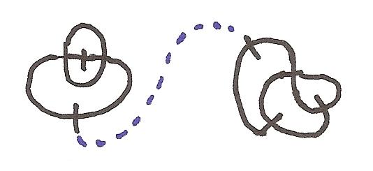
Figure 8.2: If two connected components remain, each will have a loose end on its outside, so a move remains that can connect the two. A similar argument works in the case where one connected component lies inside another.

So in the final position, $regions-components=4n-1$ because there are $4n$ loose ends. But initially, there is only one region and $n$ components, so $regions-components=1-n$. Therefore the total number of moves is $(4n-1)-(1-n)=5n-2$. So in particular, if $n$ is odd, then $5n-2$ is odd, so the first player to move will win, while if $n$ is even, then $5n-2$ is even, and so the second player will win.

To make Brussel Sprouts more interesting, we assign a final score based on the regions that arise. We give Left one point for every triangLe, and Right one point for every squaRe. We are counting a region as a “triangle” or a “square” if it has 3 or 4 corners (not counting the ones by the loose end).

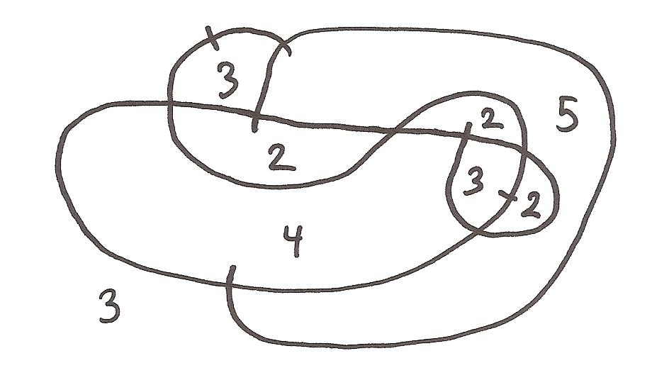
Figure 8.3: The number of “sides” of each region. Note that the outside counts as a region, in this case a triangle.

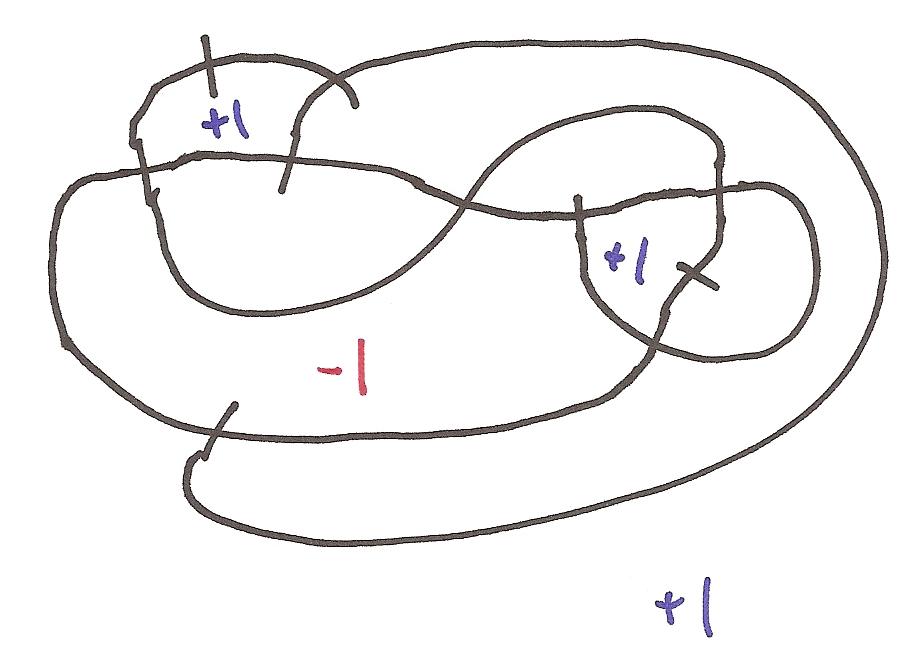
Figure 8.4: A scored version of Figure 8.3. There is one square and four triangles, so Left wins by three points.

We call this variant Scored Brussel Sprouts. Note that the game is no longer impartial, because we have introduced an asymmetry between the two players in the scoring.

Both Mercenary Clobber and Scored Brussel Sprouts have a tendency to decompose into independent positions whose scores are combined by addition:

Figure 8.5: Each circled region is an independent subgame.

In Scored Brussel Sprouts, something more drastic happens: each individual region becomes its own subgame. This makes the gamut of indecomposable positions smaller and more amenable to analysis.

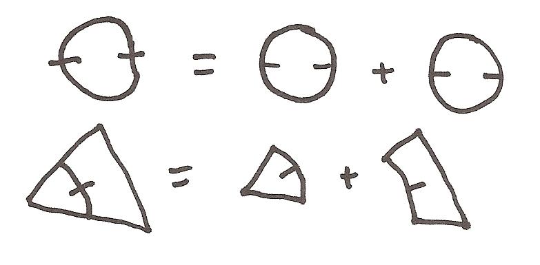
Figure 8.6: A Scored Brussel Sprouts position is the sum of its individual cells.

Because both Mercenary Clobber and Scored Brussel Sprouts decompose into independent subpositions, they will be directly amenable to the theory we develop. In contrast, To Knot or Not to Knot does not add scores, but instead combines them by a maximum, or a Boolean OR. We will see in Chapter 12 why it can still be analyzed by the theory of fixed-length scoring games and addition.

For technical reasons we will actually consider a slightly larger class of games than fixed-length games. We will study fixed-parity or well-tempered games, in which the parity of the game’s length is predetermined, rather than its exact length. In other words, these are the games where we can say at the outset which player will make the last move. While this class of games is much larger, we will see below (Corollary 9.3.6) that every fixed-parity game is equivalent to a fixed-length game, so that the resulting indistinguishability quotients are identical. I cannot think of any natural examples of games which are fixed-parity but not fixed-length, since it seems difficult to arrange for the game’s length to vary but not its parity.

By restricting to well-tempered games, we are excluding strategic concerns of getting the last move, and thus one might expect that the resulting theory would be orthogonal to the standard theory of partizan games. However, it actually turns out to closely duplicate it, as we will see in Chapter 11.

There is one more technical restriction we make: we will only consider games taking values in the integers. Milnor, Hanner, and Ettinger all considered games taking values in the full real numbers, but we will only allow integers, mainly so that Chapter 11 works out. Most of the results we prove will be equally valid for real-valued well-tempered games, and the full indistinguishability quotient of real-valued well-tempered games can be described in terms of integer-valued games using the results of Chapter 10. We leave these generalizations as an exercise to the motivated reader.

Chapter 9 Well-tempered Scoring Games

9.1 Definitions

We will focus on the following class of games:

Definition 9.1.1.

Let $\mathcal{S}\subseteq\mathbb{Z}$. Then an even-tempered $\mathcal{S}$-valued game is either an element of $\mathcal{S}$ or a pair $\langle L\,|\,R\rangle$ where $L$ and $R$ are finite nonempty sets of odd-tempered $\mathcal{S}$-valued games. An odd-tempered $\mathcal{S}$-valued game is a pair $\langle L\,|\,R\rangle$ where $L$ and $R$ are finite nonempty sets of even-tempered $\mathcal{S}$-valued games. A well-tempered $\mathcal{S}$-valued game is an even-tempered $\mathcal{S}$-valued game or an odd-tempered $\mathcal{S}$-valued game. The set of well-tempered $\mathcal{S}$-valued games is denoted $\mathcal{W}_{\mathcal{S}}$. The subsets of even-tempered and odd-tempered games are denoted $\mathcal{W}_{\mathcal{S}}^{0}$ and $\mathcal{W}_{\mathcal{S}}^{1}$, respectively. If $G=\langle L\,|\,R\rangle$, then the elements of $L$ are called the left options of $G$, and the elements of $R$ are called the right options. If $G=n$ for some $n\in\mathcal{S}$, then we say that $G$ has no left or right options. In this case, we call $G$ a number.

As usual, we omit the curly braces in $\langle\{L_{1},L_{2},\ldots\}\,|\,\{R_{1},R_{2},\ldots\}\rangle$, writing it as $\langle L_{1},L_{2},\ldots\,|\,R_{1},R_{2},\ldots\rangle$ instead. We also adopt some of the same notational conventions from partizan theory, like letting $\langle x||y|z\rangle$ denote $\langle x|\langle y|z\rangle\rangle$. We also use $*$ and $x*$ to denote $\langle 0|0\rangle$ and $\langle x|x\rangle$.

We will generally refer to well-tempered scoring games simply as “games” or “$\mathbb{Z}$-valued games” in what follows, and refer to the games of Conway’s partizan game theory as “partizan games” when we need them.

We next define outcomes.

Definition 9.1.2.

For $G\in\mathcal{W}_{\mathcal{S}}$ we define $\operatorname{L}(G)=\operatorname{R}(G)=n$ if $G=n\in\mathcal{S}$, and otherwise, if $G=\langle L_{1},L_{2},\ldots\,|\,R_{1},R_{2},\ldots\rangle$, then we define

$$\operatorname{L}(G)=\max\{\operatorname{R}(L_{1}),\operatorname{R}(L_{2}),\ldots\}$$

$$\operatorname{R}(G)=\min\{\operatorname{L}(R_{1}),\operatorname{L}(R_{2}),\ldots\}.$$

For any $G\in\mathcal{W}_{\mathcal{S}}$, $\operatorname{L}(G)$ is called the left outcome of $G$, $\operatorname{R}(G)$ is called the right outcome of $G$, and the ordered pair $(\operatorname{L}(G),\operatorname{R}(G))$ is called the (full) outcome of $G$, denoted $\operatorname{o^{\#}}(G)$.

The outcomes of a game $G$ are just the final scores of the game when Left and Right play first, and both players play perfectly. It is clear from the definition that if $G\in\mathcal{W}_{\mathcal{S}}$, then $\operatorname{o^{\#}}(G)\in\mathcal{S}\times\mathcal{S}$. We compare outcomes of games using the obvious partial order on $\mathcal{S}\times\mathcal{S}$. So for example $\operatorname{o^{\#}}(G_{1})\leq\operatorname{o^{\#}}(G_{2})$ iff $\operatorname{R}(G_{1})\leq\operatorname{R}(G_{2})$ and $\operatorname{L}(G_{1})\leq\operatorname{L}(G_{2})$. In what follows, we will use bounds like

$$\operatorname{L}(G^{R})\geq\operatorname{R}(G)\text{ for all $G^{R}$}$$

without explanation.

We next define operations on games. For $\mathcal{S},\mathcal{T}\subseteq\mathbb{Z}$, we let $\mathcal{S}+\mathcal{T}$ denote $\{s+t\,:\,s\in\mathcal{S},\,t\in\mathcal{T}\}$, and $-\mathcal{S}$ denote $\{-s\,:\,s\in\mathcal{S}\}$.

Definition 9.1.3.

If $G$ is an $\mathcal{S}$-valued game, then its negative $-G$ is the $(-\mathcal{S})$-valued game defined recursively as $-n$ if $G=n\in\mathcal{S}$, and as

$$-G=\langle-R_{1},-R_{2},\ldots\,|\,-L_{1},-L_{2},\ldots\rangle$$

if $G=\langle L_{1},L_{2},\ldots\,|\,R_{1},R_{2},\ldots\rangle$.

Negation preserves parity: the negation of an even-tempered or odd-tempered game is an even-tempered or odd-tempered game. Moreover, $-(-G)=G$ for any game $G$. It is also easy to check that $\operatorname{L}(-G)=-\operatorname{R}(G)$ and $\operatorname{R}(-G)=-\operatorname{L}(G)$.

We next define the sum of two games, in which we play the two games in parallel (like a sum of partizan games), and add together the final scores at the end.

Definition 9.1.4.

If $G$ is an $\mathcal{S}$-valued game and $H$ is a $\mathcal{T}$-valued game, then the sum $G+H$ is defined in the usual way if $G$ and $H$ are both numbers, and otherwise defined recursively as

$$G+H=\langle G+H^{L},\,G^{L}+H\,|\,G+H^{R},\,G^{R}+H\rangle$$ (9.1)

where $G^{L}$ and $G^{R}$ range over all left and right options of $G$, and $H^{L}$ and $H^{R}$ range over all left and right options of $H$.

Note that (9.1) is used even when one of $G$ and $H$ is a number but the other isn’t. For instance,

$$2+\langle 3|4\rangle=\langle 5|6\rangle.$$

In this sense, number avoidance is somehow built in to our theory.

It is easy to verify that $0+G=G=G+0$ for any $\mathbb{Z}$-valued game $G$, and that addition is associative and commutative. Moreover, the sum of two even-tempered games or two odd-tempered games is even-tempered, while the sum of an even-tempered and an odd-tempered game is odd-tempered. Another important fact which we’ll need later is the following:

Proposition 9.1.5.

If $G$ is a $\mathbb{Z}$-valued game and $n$ is a number, then

$$\operatorname{L}(G+n)=\operatorname{L}(G)+n$$

and

$$\operatorname{R}(G+n)=\operatorname{R}(G)+n.$$

Proof.

Easily seen inductively from the definition. If $G$ is a number, this is obvious, and otherwise, if $G=\langle L_{1},L_{2},\ldots\,|\,R_{1},R_{2},\ldots\rangle$, then $n$ has no options, so

$$G+n=\langle L_{1}+n,L_{2}+n,\ldots\,|\,R_{1}+n,R_{2}+n,\ldots\rangle.$$

Thus by induction

$$\operatorname{L}(G+n)=\max\{\operatorname{R}(L_{1}+n),\operatorname{R}(L_{2}+n),\ldots\}=\max\{\operatorname{R}(L_{1})+n,\operatorname{R}(L_{2})+n,\ldots\}=\operatorname{L}(G)+n,$$

and similarly $\operatorname{R}(G+n)=\operatorname{R}(G)+n$. ∎

We also define $G-H$ in the usual way, as $G+(-H)$.

9.2 Outcomes and Addition

In the theory of normal partizan games, $G\geq 0$ and $H\geq 0$ implied that $G+H\geq 0$, because Left could combine her strategies in the two games to win in their sum. Similarly, for $\mathbb{Z}$-valued games, we have the following:

Claim 9.2.1.

If $G$ and $H$ are even-tempered $\mathbb{Z}$-valued games, and $\operatorname{R}(G)\geq 0$ and $\operatorname{R}(H)\geq 0$, then $\operatorname{R}(G+H)\geq 0$.

Left combines her strategies in $G$ and $H$. Whenever Right moves in either component, Left responds in the same component, playing responsively. Similarly, just as $G\rhd 0$ and $H\geq 0$ implied $G+H\rhd 0$ for partizan games, we have

Claim 9.2.2.

If $G,H$ are $\mathbb{Z}$-valued games, with $G$ odd-tempered and $H$ even-tempered, and $\operatorname{L}(G)\geq 0$ and $\operatorname{R}(H)\geq 0$, then $\operatorname{L}(G+H)\geq 0$.

Since $G$ is odd-tempered (thus not a number) and $\operatorname{L}(G)\geq 0$, there must be some left option $G^{L}$ with $\operatorname{R}(G^{L})\geq 0$. Then by the previous claim, $\operatorname{R}(G^{L}+H)\geq 0$. So moving first, Left can ensure a final score of at least zero, by moving to $G^{L}+H$.

Of course there is nothing special about the score 0. More generally, we have

• If $G$ and $H$ are even-tempered, $\operatorname{R}(G)\geq m$ and $\operatorname{R}(H)\geq n$, then $\operatorname{R}(G+H)\geq m+n$. In other words, $\operatorname{R}(G+H)\geq\operatorname{R}(G)+\operatorname{R}(H)$.

• If $G$ is odd-tempered, $H$ is even-tempered, $\operatorname{L}(G)\geq m$, and $\operatorname{R}(H)\geq n$, then $\operatorname{L}(G+H)\geq m+n$. In other words, $\operatorname{L}(G+H)\geq\operatorname{L}(G)+\operatorname{R}(H)$.

We state these results in a theorem, and give formal inductive proofs:

Theorem 9.2.3.

Let $G$ and $H$ be $\mathbb{Z}$-valued games. If $G$ and $H$ are both even-tempered, then

$$\operatorname{R}(G+H)\geq\operatorname{R}(G)+\operatorname{R}(H)$$ (9.2)

Likewise, if $G$ is odd-tempered and $H$ is even-tempered, then

$$\operatorname{L}(G+H)\geq\operatorname{L}(G)+\operatorname{R}(H)$$ (9.3)

Proof.

Proceed by induction on the complexity of $G$ and $H$. If $G$ and $H$ are both even-tempered, then (9.2) follows from Proposition 9.1.5 whenever $G$ or $H$ is a number, so suppose both are not numbers. Then every right-option of $G+H$ is either of the form $G^{R}+H$ or $G+H^{R}$. Since $G^{R}$ is odd-tempered, by induction (9.3) tells us that $\operatorname{L}(G^{R}+H)\geq\operatorname{L}(G^{R})+\operatorname{R}(H)$. Clearly $\operatorname{L}(G^{R})+\operatorname{R}(H)\geq\operatorname{R}(G)+\operatorname{R}(H)$, because $\operatorname{R}(G)$ is the minimum value of $\operatorname{L}(G^{R})$. So $\operatorname{L}(G^{R}+H)$ is always at least $\operatorname{R}(G)+\operatorname{R}(H)$. Similarly, $\operatorname{L}(G+H^{R})$ is always at least $\operatorname{R}(G)+\operatorname{R}(H)$. So every right option of $G+H$ has left-outcome at least $\operatorname{R}(G)+\operatorname{R}(H)$, and so the best right can do with $G+H$ is $\operatorname{R}(G)+\operatorname{R}(H)$, proving (9.2).

If $G$ is odd-tempered and $H$ is even-tempered, then $G$ is not a number so there is some left option $G^{L}$ with $\operatorname{L}(G)=\operatorname{R}(G^{R})$. Then by induction, (9.2) gives

$$\operatorname{R}(G^{R}+H)\geq\operatorname{R}(G^{R})+\operatorname{R}(H)=\operatorname{L}(G)+\operatorname{R}(H).$$

But clearly $\operatorname{L}(G+H)\geq\operatorname{R}(G^{R}+H)$, so we are done. ∎

Similarly we have

Theorem 9.2.4.

Let $G$ and $H$ be $\mathbb{Z}$-valued games. If $G$ and $H$ are both even-tempered, then

$$\operatorname{L}(G+H)\leq\operatorname{L}(G)+\operatorname{L}(H)$$ (9.4)

Likewise, if $G$ is odd-tempered and $H$ is even-tempered, then

$$\operatorname{R}(G+H)\leq\operatorname{R}(G)+\operatorname{L}(H)$$ (9.5)

Another key fact in the case of partizan games was that $G+(-G)\geq 0$. Here we have the analogous fact that

Theorem 9.2.5.

If $G$ is a $\mathbb{Z}$-valued game (of either parity), then

$$\operatorname{R}(G+(-G))\geq 0$$ (9.6)

$$\operatorname{L}(G+(-G))\leq 0$$ (9.7)

Proof.

Consider the game $G+(-G)$. When Right goes first, Left has an obvious Tweedledum and Tweedledee Strategy mirroring moves in the two components, which guarantees a score of exactly zero. This play may not be optimal, but it at least shows that $\operatorname{R}(G+(-G))\geq 0$. The other case is similar. ∎

Unfortunately, some of the results above are contingent on parity. Without the conditions on parity, equations (9.2-9.5) would fail. For example, if $G$ is the even-tempered game $\langle-1|-1||1|1\rangle=\langle\langle-1|-1\rangle|\langle 1|1\rangle\rangle$ and $H$ is the odd-tempered game $\langle G\,|\,G\rangle$, then the reader can easily check that $\operatorname{R}(G)=1$, $\operatorname{R}(H)=-1$, but $\operatorname{R}(G+H)=-2$ (Right moves from $H$ to $G$), and $-2\not\geq 1+(-1)$, so that (9.2) fails. The problem here is that since $H$ is odd-tempered, Right can end up making the last move in $H$, and then Left is forced to move in $G$, breaking her strategy of only playing responsively.

To amend this situation, we consider a restricted class of games, in which being forced to unexpectedly move is not harmful.

Definition 9.2.6.

An i-game is a $\mathbb{Z}$-valued game $G$ which has the property that every option is an i-game, and if $G$ is even-tempered, then $\operatorname{L}(G)\geq\operatorname{R}(G)$.

So for instance, numbers are always i-games, $*$ and $1*$ and even $\langle-1|1\rangle$ are i-games, but the game $G=\langle-1+*\,|\,1+*\rangle$ mentioned above is not, because it is even-tempered and $\operatorname{L}(G)=-1<1=\operatorname{R}(G)$. It may seem arbitrary that we only require $\operatorname{L}(G)\geq\operatorname{R}(G)$ when $G$ is even-tempered, but later we will see that this definition is more natural than it might first appear.

Now we can extend Claim 9.2.1 to the following:

Claim 9.2.7.

If $G$ and $H$ are $\mathbb{Z}$-valued games, $G$ is even-tempered and an i-game, $H$ is odd-tempered, and $\operatorname{R}(G)\geq 0$ and $\operatorname{R}(H)\geq 0$, then $\operatorname{R}(G+H)\geq 0$.

In this case, Left is again able to play responsively in each component, but in the situation where Right makes the final move in the second component, Left is able to leverage the fact that the first component’s left-outcome is at least its right-outcome, because the first component will be an even-tempered i-game. And similarly, we also have

Claim 9.2.8.

If $G$ and $H$ are odd-tempered $\mathbb{Z}$-valued games, $G$ is an i-game, $\operatorname{L}(G)\geq 0$ and $\operatorname{R}(H)\geq 0$, then $\operatorname{L}(G+H)\geq 0$. If $G$ and $H$ are even-tempered $\mathbb{Z}$-valued games, $G$ is an i-game, $\operatorname{R}(G)\geq 0$ and $\operatorname{L}(H)\geq 0$, then $\operatorname{L}(G+H)\geq 0$.

As before, these results can be generalized to the following:

Theorem 9.2.9.

Let $G$ and $H$ be $\mathbb{Z}$-valued games, and $G$ an i-game.

• If $G$ is even-tempered and $H$ is odd-tempered, then

  $$\operatorname{R}(G+H)\geq\operatorname{R}(G)+\operatorname{R}(H)$$ (9.8)

• If $G$ and $H$ are both odd-tempered, then

  $$\operatorname{L}(G+H)\geq\operatorname{L}(G)+\operatorname{R}(H)$$ (9.9)

• If $G$ and $H$ are both even-tempered, then

  $$\operatorname{L}(G+H)\geq\operatorname{R}(G)+\operatorname{L}(H)$$ (9.10)

Proof.

We proceed by induction on $G$ and $H$. If $G$ or $H$ is a number, then every equation follows from Proposition 9.1.5 and the stipulation that $\operatorname{L}(G)\geq\operatorname{R}(G)$ if $G$ is even-tempered. So suppose that $G$ and $H$ are both not numbers.

To see (9.8), note that every right option of $G+H$ is either of the form $G^{R}+H$ or $G+H^{R}$. Since $\operatorname{L}(G^{R})\geq\operatorname{R}(G)$ and $G^{R}$ is an odd-tempered i-game, (9.9) tells us inductively that

$$\operatorname{L}(G^{R}+H)\geq\operatorname{L}(G^{R})+\operatorname{R}(H)\geq\operatorname{R}(G)+\operatorname{R}(H).$$

And likewise since $\operatorname{L}(H^{R})\geq\operatorname{R}(H)$ and $H^{R}$ is even-tempered, (9.10) tells us inductively that

$$\operatorname{L}(G+H^{R})\geq\operatorname{R}(G)+\operatorname{L}(H^{R})\geq\operatorname{R}(G)+\operatorname{R}(H).$$

So no matter how Right moves in $G+H$, he produces a position with left-outcome at least $\operatorname{R}(G)+\operatorname{R}(H)$. This establishes (9.8).

Equations (9.9 - 9.10) can easily be seen by having Left make an optimal move in $G$ or $H$, respectively, and using (9.8) inductively. I leave the details to the reader. ∎

Similarly we have

Theorem 9.2.10.

Let $G$ and $H$ be $\mathbb{Z}$-valued games, and $G$ an i-game.

• If $G$ is even-tempered and $H$ is odd-tempered, then

  $$\operatorname{L}(G+H)\leq\operatorname{L}(G)+\operatorname{L}(H)$$ (9.11)

• If $G$ and $H$ are both odd-tempered, then

  $$\operatorname{R}(G+H)\leq\operatorname{R}(G)+\operatorname{L}(H)$$ (9.12)

• If $G$ and $H$ are both even-tempered, then

  $$\operatorname{R}(G+H)\leq\operatorname{L}(G)+\operatorname{R}(H)$$ (9.13)

As an application of this pile of inequalities, we prove some useful results about i-games.

Theorem 9.2.11.

If $G$ and $H$ are i-games, then $-G$ and $G+H$ are i-games.

Proof.

Negation is easy, and left to the reader as an exercise. We show $G+H$ is an i-game inductively. For the base case, $G$ and $H$ are both numbers, so $G+H$ is one too, and is therefore an i-game. Otherwise, by induction, every option of $G+H$ is an i-game, so it remains to show that $\operatorname{L}(G+H)\geq\operatorname{R}(G+H)$ if $G+H$ is even-tempered. In this case $G$ and $H$ have the same parity. If both are even-tempered, then by equations (9.10) and (9.13), we have

$$\operatorname{R}(G+H)\leq\operatorname{L}(G)+\operatorname{R}(H)\leq\operatorname{L}(G+H),$$

and if both are odd-tempered the same follows by equations (9.9) and (9.12) instead. ∎

Theorem 9.2.12.

If $G$ is an i-game, then $G+(-G)$ is an i-game and

$$\operatorname{L}(G+(-G))=\operatorname{R}(G+(-G))=0.$$

Proof.

We know in general, by equations (9.6-9.7), that

$$\operatorname{L}(G+(-G))\leq 0\leq\operatorname{R}(G+(-G)).$$

By the previous theorem we know that $G+(-G)$ is an i-game, and it is clearly even-tempered, so

$$\operatorname{L}(G+(-G))\geq\operatorname{R}(G+(-G))$$

and we are done. ∎

Theorem 9.2.13.

If $G$ is an even-tempered i-game, and $\operatorname{R}(G)\geq 0$, then for any $X\in\mathcal{W}_{\mathbb{Z}}$, we have $\operatorname{o^{\#}}(G+X)\geq\operatorname{o^{\#}}(X)$.

Proof.

If $X$ is even-tempered, then by Equation (9.2),

$$\operatorname{R}(X)\leq\operatorname{R}(G)+\operatorname{R}(X)\leq\operatorname{R}(G+X),$$

and by Equation (9.10) we have

$$\operatorname{L}(X)\leq\operatorname{R}(G)+\operatorname{L}(X)\leq\operatorname{L}(G+X).$$

If $X$ is odd-tempered, then by Equation (9.8),

$$\operatorname{R}(X)\leq\operatorname{R}(G)+\operatorname{R}(X)\leq\operatorname{R}(G+X),$$

and by Equation (9.3) we have

$$\operatorname{L}(X)\leq\operatorname{R}(G)+\operatorname{L}(X)\leq\operatorname{L}(G+X).$$

∎

Theorem 9.2.14.

If $G$ is an even-tempered i-game, and $\operatorname{L}(G)\leq 0$, the for any $X\in\mathcal{W}_{\mathbb{Z}}$, we have $\operatorname{o^{\#}}(G+X)\leq\operatorname{o^{\#}}(X)$.

Proof.

Analogous to Theorem 9.2.13. ∎

Theorem 9.2.15.

If $G$ is an even-tempered i-game, and $\operatorname{L}(G)=\operatorname{R}(G)=0$, then for any $X\in\mathcal{W}_{\mathbb{Z}}$, we have $\operatorname{o^{\#}}(G+X)=\operatorname{o^{\#}}(X)$.

Proof.

Combine Theorems 9.2.13 and 9.2.14. ∎

This last result suggests that if $G$ is an even-tempered i-game with vanishing outcomes, then $G$ behaves very much like $0$. Let us investigate this indistinguishability further…

9.3 Partial orders on integer-valued games

Definition 9.3.1.

If $G_{1},G_{2}\in\mathcal{W}_{\mathbb{Z}}$, then we say that $G_{1}$ and $G_{2}$ are equivalent, denoted $G_{1}\approx G_{2}$, iff $\operatorname{o^{\#}}(G_{1}+X)=\operatorname{o^{\#}}(G_{2}+X)$ for all $X\in\mathcal{W}_{\mathbb{Z}}$. We also define a preorder on $\mathcal{W}_{\mathbb{Z}}$ by $G_{1}\lesssim G_{2}$ iff $\operatorname{o^{\#}}(G_{1}+X)\leq\operatorname{o^{\#}}(G_{2}+X)$ for all $X\in\mathcal{W}_{\mathbb{Z}}$.

So in particular, $G_{1}\approx G_{2}$ iff $G_{1}\gtrsim G_{2}$ and $G_{1}\lesssim G_{2}$. Taking $X=0$ in the definitions, we see that $G_{1}\approx G_{2}$ implies $\operatorname{o^{\#}}(G_{1})=\operatorname{o^{\#}}(G_{2})$, and similarly, $G_{1}\gtrsim G_{2}$ implies that $\operatorname{o^{\#}}(G_{1})\geq\operatorname{o^{\#}}(G_{2})$. It is straightforward to see that $\approx$ is indeed an equivalence relation, and a congruence with respect to addition and negation, so that the quotient space $\mathcal{W}_{\mathbb{Z}}/\approx$ retains its commutative monoid structure. If two games $G_{1}$ and $G_{2}$ are equivalent, then they are interchangeable in all context involving addition. Later we’ll see that they’re interchangeable in all contexts made of weakly-order preserving functions. Our main goal is to understand the quotient space $\mathcal{W}_{\mathbb{Z}}/\approx$.

We restate the results at the end of last section in terms of $\approx$ and its quotient space:

Corollary 9.3.2.

If $G$ is an even-tempered i-game, then $G\lesssim 0$ iff $\operatorname{L}(G)\leq 0$, $G\gtrsim 0$ iff $\operatorname{R}(G)\geq 0$, and $G\approx 0$ iff $\operatorname{L}(G)=\operatorname{R}(G)=0$. Also, if $G$ is any i-game, then $G+(-G)\approx 0$, so every i-game is invertible modulo $\approx$ with inverse given by negation.

Proof.

Theorems 9.2.13, 9.2.14, and 9.2.15 give the implications in the direction $\Leftarrow$. For the reverse directions, note that if $G\lesssim 0$, then by definition $\operatorname{L}(G+0)\leq\operatorname{L}(0+0)=0$. And similarly $G\gtrsim 0$ implies $\operatorname{R}(G)\geq 0$, and $G\approx 0$ implies $\operatorname{o^{\#}}(G)=\operatorname{o^{\#}}(0)$. For the last claim, note that by Theorem 9.2.12, $G+(-G)$ has vanishing outcomes, so by what has just been shown $G+(-G)\approx 0$. ∎

Note that this gives us a test for $\approx$ and $\lesssim$ between i-games: $G\lesssim H$ iff $G+(-H)\lesssim H+(-H)\approx 0$, iff $\operatorname{L}(G+(-H))\leq 0$. Here we have used the fact that $G\lesssim H$ implies $G+X\lesssim H+X$, which is easy to see from the definition. And if $X$ is invertible, then the implication holds in the other direction.

Also, by combining Corollary 9.3.2, and Theorem 9.2.11, we see that i-games modulo $\approx$ are an abelian group, partially ordered by $\lesssim$.

We next show that even-tempered and odd-tempered games are never comparable.

Theorem 9.3.3.

If $G_{1},G_{2}\in\mathcal{W}_{\mathbb{Z}}$ but $G_{1}$ is odd-tempered and $G_{2}$ is even-tempered, then $G_{1}$ and $G_{2}$ are incomparable with respect to the $\gtrsim$ preorder. Thus no two games of differing parity are equivalent.

Proof.

Since we are only considering finite games, there is some $N\in\mathbb{Z}$ such that $N$ is greater in magnitude than all numbers occuring within $G_{1}$ and $G_{2}$. Since $\langle-N|N\rangle\in\mathcal{W}_{\mathbb{Z}}$, it suffices to show that $\operatorname{L}(G_{1}+\langle-N|N\rangle)$ is positive while $\operatorname{L}(G_{2}+\langle-N|N\rangle)$ is negative. In both sums, $G_{1}+\langle-N\,|\,N\rangle$ and $G_{2}+\langle-N\,|\,N\rangle$, $N$ is so large that no player will move in $\langle-N\,|\,N\rangle$ unless they have no other alternative. Moreover, the final score will be positive iff Right had to move in this component, and negative iff Left had to move in this component, because $N$ is so large that it dwarves the score of the other component. Consequently, we can assume that the last move of the game will be in the $\langle-N\,|\,N\rangle$ component. Since $G_{1}+\langle-N|N\rangle$ is even-tempered, Right will make the final move if Left goes first, so $\operatorname{L}(G_{1}+\langle-N\,|\,N\rangle)>0$. But on the other hand, $G_{2}+\langle-N|N\rangle$ is odd-tempered, so Left will make the final move if Left goes first, and therefore $\operatorname{L}(G_{2}+\langle-N\,|\,N\rangle)<0$, so we are done. ∎

Thus $\mathcal{W}_{\mathbb{Z}}/\approx$ is naturally the disjoint union of its even-tempered and odd-tempered components: $\mathcal{W}_{\mathbb{Z}}^{0}/\approx$ and $\mathcal{W}_{\mathbb{Z}}^{1}/\approx$.

Although they are incomparable with each other, $\mathcal{W}_{\mathbb{Z}}^{0}$ and $\mathcal{W}_{\mathbb{Z}}^{1}$ are very closely related, as the next results show:

Theorem 9.3.4.

Let $*$ be $\langle 0|0\rangle$. If $G\in\mathcal{W}_{\mathbb{Z}}$, then $G+*+*\approx G$. The map $G\to G+*$ establishes an involution on $\mathcal{W}_{\mathbb{Z}}/\approx$ interchanging $\mathcal{W}_{\mathbb{Z}}^{0}/\approx$ and $\mathcal{W}_{\mathbb{Z}}^{1}/\approx$. In fact, as a commutative monoid, $\mathcal{W}_{\mathbb{Z}}$ is isomorphic to the direct product of the cyclic group $\mathbb{Z}_{2}$ and the submonoid $\mathcal{W}_{\mathbb{Z}}^{0}/\approx$.

Proof.

It’s clear that $*$ is an i-game, and it is its own negative, so that $*+*\approx 0$. Therefore $G+*+*\approx G$ for any $G$. Because $\approx$ is a congruence with respect to addition, $G\to G+*$ is a well-defined map on $\mathcal{W}_{\mathbb{Z}}/\approx$. Because $*$ is odd-tempered, this map will certainly interchange even-tempered and odd-tempered games. It is an involution by the first claim. Then, since every $\overline{G}\in\mathcal{W}_{\mathbb{Z}}/\approx$ is of the form $\overline{H}$ or $\overline{H}+\overline{*}$, and since $\overline{*}+\overline{*}=\overline{0+*+*}=\overline{0}$, the desired direct sum decomposition follows. ∎

As a corollary, we see that every fixed-parity (well-tempered) game is equivalent to a fixed-length game:

Definition 9.3.5.

Let $G$ be a well-tempered scoring game. Then $G$ has length 0 if $G$ is a number, and has length $n+1$ if every option of $G$ has length 0. A well-tempered game is fixed-length if it has length $n$ for any $n$.

It is easy to see by induction that if $G$ and $H$ have lengths $n$ and $m$, then $G+H$ has length $n+m$.

Corollary 9.3.6.

Every well-tempered game $G$ is equivalent ($\approx$) to a fixed-length game.

Proof.

We prove the following claims by induction on $G$:

• If $G$ is even-tempered, then for all large enough even $n$, $G\approx H$ for some game $H$ of length $n$.

• If $G$ is odd-tempered, then for all large enough odd $n$, $G\approx H$ for some game $H$ of length $n$.

If $G$ is a number, then $G$ is even-tempered. By definition, $G$ already has length 0. On the other hand, $*$ has length 1, so $G+*+*$ has length 2, $G+*+*+*+*$ has length 4, and so on. By Theorem 9.3.4, these games are all equivalent to $G$. This establishes the base case.

For the inductive step, suppose that $G=\langle A,B,C,\ldots|D,E,F,\ldots\rangle$. If $G$ is even-tempered, then $A,B,C,\ldots,D,E,F,\ldots$ are all odd-tempered. By induction, we can find length $n-1$ games $A^{\prime},B^{\prime},\ldots$ with

$$A\approx A^{\prime},$$

$$B\approx B^{\prime},$$

and so on, for all large enough even $n$. By Theorem 9.4.4 below, we then have

$$G=\langle A,B,C,\ldots|D,E,F,\ldots\rangle\approx\langle A^{\prime},B^{\prime},C^{\prime},\ldots|D^{\prime},E^{\prime},F^{\prime},\ldots\rangle,$$

where $H=\langle A^{\prime},B^{\prime},C^{\prime},\ldots|D^{\prime},E^{\prime},F^{\prime},\ldots\rangle$ has length $n$. So $G$ is equivalent to a game of length $n$, for large enough even $n$. The case where $G$ is odd-tempered is handled in a completely analogous way. ∎

Because of this corollary, the indistinguishability quotient of well-tempered games is the same as the indistinguishability quotient of fixed-length games.

Unfortunately our definition of $\approx$ is difficult to use in practice, between non-i-games, since we have to check all $X\in\mathcal{W}_{\mathbb{Z}}$. Perhaps we can come up with a better equivalent definition?

9.4 Who goes last?

The outcome of a partizan game or a $\mathbb{Z}$-valued game depends on which player goes first. However, since our $\mathbb{Z}$-valued games are fixed-parity games, saying who goes first is the same as saying who goes last. We might as well consider the following:

Definition 9.4.1.

The left-final outcome $\operatorname{Lf}(G)$ of a $\mathcal{S}$-valued game $G$ is the outcome of $G$ when Left makes the final move, and the right-final outcome $\operatorname{Rf}(G)$ is the outcome when Right makes the final move. In other words, if $G$ is odd-tempered (whoever goes first also goes last), then

$$\operatorname{Lf}(G)=\operatorname{L}(G)$$

$$\operatorname{Rf}(G)=\operatorname{R}(G)$$

while if $G$ is even-tempered, then

$$\operatorname{Lf}(G)=\operatorname{R}(G)$$

$$\operatorname{Rf}(G)=\operatorname{L}(G).$$

This may seem arbitrary, but it turns out to be the key to understanding well-tempered scoring games. We will see in Section 9.5 that a $\mathbb{Z}$-valued game is schizophrenic in nature, acting as one of two different i-games depending on which player will make the final move. With this in mind, we make the following definitions:

Definition 9.4.2.

(Left’s partial order) If $G$ and $H$ are two $\mathbb{Z}$-valued games of the same parity, we define $G\lesssim_{+}H$ if $\operatorname{Lf}(G+X)\leq\operatorname{Lf}(H+X)$ for all $X\in\mathcal{W}_{\mathbb{Z}}$, and $G\approx_{+}H$ if $\operatorname{Lf}(G+X)=\operatorname{Lf}(H+X)$ for all $X\in\mathcal{W}_{\mathbb{Z}}$.

Definition 9.4.3.

(Right’s partial order) If $G$ and $H$ are two $\mathbb{Z}$-valued games of the same parity, we define $G\lesssim_{-}H$ if $\operatorname{Rf}(G+X)\leq\operatorname{Rf}(H+X)$ for all $X\in\mathcal{W}_{\mathbb{Z}}$, and $G\approx_{-}H$ if $\operatorname{Rf}(G+X)=\operatorname{Rf}(H+X)$ for all $X\in\mathcal{W}_{\mathbb{Z}}$.

It is clear that $\lesssim_{\pm}$ are preorders and $\approx_{\pm}$ are equivalence relations, and that $G\lesssim H$ iff $G\lesssim_{+}H$ and $G\lesssim_{-}H$, and that $G\approx H$ iff $G\approx_{+}H$ and $G\approx_{-}H$, in light of Theorem 9.3.3. Also, $\approx_{\pm}$ are still congruences with respect to addition (though not negation), i.e., if $G\approx_{+}G^{\prime}$ and $H\approx_{+}H^{\prime}$, then $G+H\approx_{+}G^{\prime}+H^{\prime}$.

All three equivalence relations are also congruences with respect to the operation of game formation. In fact, we have

Theorem 9.4.4.

Let $\Box$ be one of $\approx$, $\approx_{+}$, $\approx_{-}$, $\lesssim$, $\lesssim_{+}$, $\lesssim_{-}$, $\gtrsim$, $\gtrsim_{-}$, or $\gtrsim_{+}$. Suppose that $L_{1}\ \Box\ L_{1}^{\prime}$, $L_{2}\ \Box\ L_{2}^{\prime}$, …, $R_{1}\ \Box\ R_{1}^{\prime}$, $R_{2}\ \Box R_{2}^{\prime}$, …. Then

$$\langle L_{1},L_{2},\ldots\ |\ R_{1},R_{2},\ldots\rangle\ \Box\ \langle L_{1}^{\prime},L_{2}^{\prime},\ldots\ |\ R_{1}^{\prime},R_{2}^{\prime},\ldots\rangle.$$

Proof.

All have obvious inductive proofs. For example, suppose $\Box$ is $\lesssim_{-}$. Let $G=\langle L_{1},L_{2},\ldots\ |\ R_{1},R_{2},\ldots\rangle$ and $H=\langle L_{1}^{\prime},L_{2}^{\prime},\ldots\ |\ R_{1}^{\prime},R_{2}^{\prime},\ldots\rangle$. Then for any $X\in\mathcal{W}_{\mathbb{Z}}$, if $G+X$ is even-tempered then

$$\operatorname{Lf}(G+X)=\min\{\operatorname{Lf}(G^{R}+X),\operatorname{Lf}(G+X^{R})\}\leq\min\{\operatorname{Lf}(H^{R}+X),\operatorname{Lf}(H+X^{R})\},$$

where the inequality follows by induction, and if $G+X$ is odd-tempered, then

$$\operatorname{Lf}(G+X)=\max\{\operatorname{Lf}(G^{L}+X),\operatorname{Lf}(G+X^{L})\}\leq\max\{\operatorname{Lf}(H^{L}+X),\operatorname{Lf}(H+X^{L})\}.$$

Note that the induction is on $G$, $H$, and $X$ all together. ∎

The next four lemmas are key:

Lemma 9.4.5.

If $G,H\in\mathcal{W}_{\mathbb{Z}}$ and $H$ is an i-game, then $G\lesssim H\iff G\lesssim_{+}H$.

Proof.

The direction $\Rightarrow$ is obvious. So suppose that $G\lesssim_{+}H$. Since $H$ is invertible modulo $\approx$ and therefore $\approx_{+}$, assume without loss of generality that $H$ is zero. In this case, we are given that $G$ is even-tempered and $\operatorname{Lf}(G+X)\leq\operatorname{Lf}(X)$ for every $X\in\mathcal{W}_{\mathbb{Z}}$, and we want to show $\operatorname{Rf}(G+X)\leq\operatorname{Rf}(X)$ for every $X\in\mathcal{W}_{\mathbb{Z}}$. Taking $X=-G$, we see by Equation (9.6) above that

$$0\leq\operatorname{R}(G+(-G))=\operatorname{Lf}(G+X)\leq\operatorname{Lf}(-G)=-\operatorname{Rf}(G)=-\operatorname{L}(G),$$

so that

$$\operatorname{L}(G)\leq 0.$$

Now let $X$ be arbitrary. If $X$ is even-tempered, then by Equation (9.4)

$$\operatorname{Rf}(G+X)=\operatorname{L}(G+X)\leq\operatorname{L}(G)+\operatorname{L}(X)\leq\operatorname{L}(X)=\operatorname{Rf}(X).$$

Otherwise, by Equation (9.5)

$$\operatorname{Rf}(G+X)=\operatorname{R}(G+X)\leq\operatorname{L}(G)+\operatorname{R}(X)\leq\operatorname{R}(X)=\operatorname{Rf}(X).$$

∎

Lemma 9.4.6.

If $G,H\in\mathcal{W}_{\mathbb{Z}}$ and $G$ is an i-game, then $G\lesssim H\iff G\lesssim_{-}H$.

Proof.

Analogous to the previous lemma. ∎

Proposition 9.4.7.

If $G$ and $H$ are i-games, then $G\lesssim H\iff G\lesssim_{-}H\iff G\lesssim_{+}H$.

Proof.

Follows directly from the preceding two lemmas. ∎

With Corollary 9.3.2, this gives us a way of testing $\lesssim_{\pm}$ between i-games, but it doesn’t seem to help us compute $\lesssim$ for arbitrary games!

Lemma 9.4.8.

If $G$ is an even-tempered $\mathbb{Z}$-valued game, and $n$ is an integer, then $G\lesssim_{-}n$ iff $\operatorname{L}(G)\leq n$. Similarly, $n\lesssim_{+}G$ iff $\operatorname{R}(G)\geq n$.

Proof.

First, note that if $G\lesssim_{-}n$, then certainly $\operatorname{L}(G)=\operatorname{Rf}(G+0)\leq\operatorname{Rf}(n+0)=n$. Conversely, suppose that $\operatorname{L}(G)\leq n$. Let $X$ be arbitrary. If $X$ is even-tempered then by Proposition 9.1.5 and Equation (9.4),

$$\operatorname{Rf}(G+X)=\operatorname{L}(G+X)\leq\operatorname{L}(G)+\operatorname{L}(X)\leq n+\operatorname{L}(X)=\operatorname{Rf}(n+X).$$

If $X$ is odd-tempered, we use Equation (9.5) instead:

$$\operatorname{Rf}(G+X)=\operatorname{R}(G+X)\leq\operatorname{L}(G)+\operatorname{R}(X)\leq n+\operatorname{R}(X)=\operatorname{Rf}(n+X).$$

So for every $X$, $\operatorname{Rf}(G+X)\leq\operatorname{Rf}(n+X)$ and we have shown the first sentence. The second is proven analogously. ∎

Lemma 9.4.9.

Let $G$ be an even-tempered game, whose options are all i-games. If $\operatorname{L}(G)\leq\operatorname{R}(G)$, then $G\approx_{-}\operatorname{L}(G)$ and $G\approx_{+}\operatorname{R}(G)$.

Proof.

We show $G\approx_{-}\operatorname{L}(G)$, because the other result follows by symmetry. Let $n=\operatorname{L}(G)$. Now since $\operatorname{L}(G)\leq n$, we have $G\lesssim_{-}n$ by the preceding lemma, so it remains to show that $n=\lesssim_{-}G$. If $G$ is a number, it must be $n$, and we are done. Otherwise, by definition of $\operatorname{L}$, it must be the case that every $G^{L}$ satisfies $\operatorname{R}(G^{L})\leq n$.

Let $X$ be an arbitrary game. We show by induction on $X$ that $n+\operatorname{Rf}(X)\leq\operatorname{Rf}(G+X)$. (This suffices because $n+\operatorname{Rf}(X)=\operatorname{Rf}(n+X)$.) If $X$ is even-tempered, then we need to show

$$n+\operatorname{L}(X)\leq\operatorname{L}(G+X).$$

This is obvious if $X$ is a number (since then $\operatorname{L}(G+X)=\operatorname{L}(G)+\operatorname{L}(X)$), so suppose $X$ is not a number. Then there is some left option $X^{L}$ of $X$ with $\operatorname{L}(X)=\operatorname{R}(X^{L})$, and by the inductive hypothesis applied to $X^{L}$,

$$n+\operatorname{L}(X)=n+\operatorname{R}(X^{L})\leq\operatorname{R}(G+X^{L})\leq\operatorname{L}(G+X),$$

where the last inequality follows because $G+X^{L}$ is a left option in $G+X$.

Alternatively, if $X$ is odd-tempered, we need to show that

$$n+\operatorname{R}(X)\leq\operatorname{R}(G+X).$$

We show that every right option of $G+X$ has left outcome at least $n+\operatorname{R}(X)$. The first kind of right option is of the form $G^{R}+X$. By assumption, $\operatorname{L}(G^{R})\geq\operatorname{R}(G)\geq\operatorname{L}(G)=n$, and $G^{R}$ is an odd-tempered i-game, so by Equation (9.9)

$$\operatorname{L}(G^{R}+X)\geq\operatorname{L}(G^{R})+\operatorname{R}(X)\geq n+\operatorname{R}(X).$$

The second kind of right option is of the form $G+X^{R}$. By induction we know that

$$n+\operatorname{R}(X)\leq n+\operatorname{L}(X^{R})\leq\operatorname{L}(G+X^{R}),$$

So every right option of $G+X$ has left outcome at least $n+R(X)$, and we are done. ∎

9.5 Sides

We now put everything together.

Theorem 9.5.1.

If $G$ is any $\mathbb{Z}$-valued game, then there exist i-games $G^{-}$ and $G^{+}$ such that $G\approx_{-}G^{-}$ and $G\approx_{+}G^{+}$, These games are unique, modulo $\approx$.

Proof.

We prove that $G^{+}$ exists, by induction on $G$. If $G$ is a number, this is obvious, taking $G^{+}=G$. Otherwise, let $G=\langle L_{1},L_{2},\ldots\,|\,R_{1},R_{2},\ldots\rangle$. By induction, $L_{i}^{+}$ and $R_{i}^{+}$ exist. Consider the game

$$H=\langle L_{1}^{+},L_{2}^{+},\ldots\,|\,R_{1}^{+},R_{2}^{+},\ldots\rangle.$$

By the inductive assumptions and Theorem 9.4.4, we clearly have $H\approx_{+}G$. However, $H$ might not be an i-game. This can only happen if $G$ and $H$ are even-tempered, and $\operatorname{L}(H)<\operatorname{R}(H)$. In this case, by Lemma 9.4.9, $\operatorname{R}(H)\approx_{+}H\approx_{+}G$, and $\operatorname{R}(H)$ is a number, so take $G^{+}=\operatorname{R}(H)$.

A similar argument shows that $G^{-}$ exists. Uniqueness follows by Proposition 9.4.7. ∎

The games $G^{+}$ and $G^{-}$ in the theorem are called the upside and downside of $G$, respectively, because they have formal similarities with the “onside” and “offside” of loopy partizan game theory. An algorithm for producing the upside and downside can be extracted from the proof of the theorem.

Here are the key facts about these games

Theorem 9.5.2.

   

(a)

If $G$ and $H$ are $\mathbb{Z}$-valued games, then $G\lesssim_{-}H$ iff $G^{-}\lesssim H^{-}$, and $G\lesssim_{+}H$ iff $G^{+}\lesssim H^{+}$.

(b)

If $G$ is an i-game, then $G^{+}\approx G^{-}\approx G$.

(c)

If $G$ is a $\mathbb{Z}$-valued game, then $(-G)^{-}\approx-(G^{+})$ and $(-G)^{+}\approx-(G^{-})$.

(d)

If $G$ and $H$ are $\mathbb{Z}$-valued games,then $(G+H)^{+}\approx G^{+}+H^{+}$ and $(G+H)^{-}\approx G^{-}+H^{-}$.

(e)

For any $G$, $G^{-}\lesssim G\lesssim G^{+}$.

(f)

For any $G$, $G$ is invertible modulo $\approx$ iff it is equivalent to an i-game, iff $G^{+}\approx G^{-}$. When $G$ has an inverse, it is given by $-G$.

(g)

If $\mathcal{S}\subset\mathbb{Z}$ and $G$ is an $\mathcal{S}$-valued game, then $G^{+}$ and $G^{-}$ can be taken to be $\mathcal{S}$-valued games too.

(h)

If $G$ is even-tempered, then $\operatorname{L}(G)=\operatorname{L}(G^{-})$, and this is the smallest $n$ such that $G^{-}\lesssim n$. Similarly, $\operatorname{R}(G)=\operatorname{R}(G^{+})$, and this is the biggest $n$ such that $n\lesssim G^{+}$.

(i)

If $G$ is odd-tempered, then $\operatorname{L}(G)=\operatorname{L}(G^{+})$ and $\operatorname{R}(G)=\operatorname{R}(G^{-})$.

Proof.

   

(a)

Since $G^{-}\approx_{-}G$ and $H^{-}\approx_{-}H$, it’s clear that $G^{-}\lesssim_{-}H^{-}$ iff $G\lesssim_{-}H$. But by Proposition 9.4.7, $G^{-}\lesssim_{-}H^{-}\iff G^{-}\lesssim H^{-}$, because $G^{-}$ and $H^{-}$ are i-games. The other case is handled similarly.

(b)

By definition, $G^{-}\approx_{-}G$. But since both are i-games, Proposition 9.4.7 implies that $G^{-}\approx G$. The other case is handled similarly.

(c)

Obvious by symmetry. This can be proven by noting that $A\approx_{-}B$ iff $(-A)\approx_{+}(-B)$.

(d)

Note that since $\approx_{+}$ is a congruence with respect to addition, we have

$$(G+H)^{+}\approx_{+}(G+H)\approx_{+}G^{+}+H^{+}.$$

But since i-games are closed under addition (Theorem 9.2.11), $G^{+}+H^{+}$ is an i-game, and since $(G+H)^{+}$ is too, Proposition 9.4.7 shows that $(G+H)^{+}\approx G^{+}+H^{+}$. The other case is handled similarly.

(e)

By definition $G\approx_{+}G^{+}$, so $G\lesssim_{+}G^{+}$. But $G^{+}$ is an i-game, so by Lemma 9.4.5, $G\lesssim G^{+}$. The other case is handled similarly.

(f)

We already showed in part (b) that if $G$ is an i-game, then $G^{+}\approx G^{-}$. Conversely, if $G^{+}\approx G^{-}$, then $G\approx_{+}G^{+}$ and $G\approx_{-}G^{-}\approx G^{+}$, so $G\approx_{\pm}G^{+}$, so $G$ is equivalent to the i-game $G^{+}$. Moreover, we showed in Corollary 9.3.2 that i-games are invertible. Conversely, suppose that $G$ is invertible. Define the deficit $\operatorname{def}(G)$ to be the i-game $G^{+}-G^{-}$. This is an even-tempered i-game. By part (e), $\operatorname{def}(G)\gtrsim 0$, and by part (d), $\operatorname{def}(G+H)\approx\operatorname{def}(G)+\operatorname{def}(H)$. By part (b), $\operatorname{def}(G)\approx 0$ when $G$ is an i-game. Now suppose that $G$ is invertible, and $G+H\approx 0$. Then $\operatorname{def}(G+H)\approx\operatorname{def}(G)+\operatorname{def}(H)\approx 0$. Since i-games are a partially ordered abelian group, it follows that $0\lesssim\operatorname{def}(G)\approx-\operatorname{def}(H)\lesssim 0$, so that $\operatorname{def}(G)\approx 0$, or in other words, $G^{+}\approx G^{-}$. This then implies that $G$ is equivalent to an i-game.

If $G$ has an inverse, then $G$ is equivalent to an i-game, so the inverse of $G$ is $-G$, by Corollary 9.3.2.

(g)

This is clear from the construction of $G^{+}$ and $G^{-}$ given in Theorem 9.5.1. At some points, we replace a game by one of its outcomes. However, the outcome of an $\mathcal{S}$-valued game is always in $\mathcal{S}$, so this doesn’t create any new outcomes.

(h)

Since $G^{-}\approx_{-}G$, it follows that $\operatorname{L}(G^{-})=\operatorname{Rf}(G^{-})=\operatorname{Rf}(G)=\operatorname{L}(G)$. Then by Lemma 9.4.8, $\operatorname{L}(G)$ is the smallest $n$ such that $G\lesssim_{-}n$, which by part (a) is the smallest $n$ such that $G^{-}\lesssim n$. The other case is handled similarly.

(i)

Since $G^{+}\approx_{+}G$, it follows that $\operatorname{L}(G^{+})=\operatorname{Lf}(G^{+})=\operatorname{Lf}(G)=\operatorname{L}(G)$. The other case is handled similarly.

∎

Borrowing notation from loopy partizan theory, we use $A\&B$ to denote a well-tempered game that has $A$ as its upside and $B$ as its downside. By Theorem 9.5.2(a), $A\&B$ is well-defined modulo $\approx$, as long as it exists: if $G^{+}\approx H^{+}$ and $G^{-}\approx H^{-}$, then $G\approx_{+}H$ and $G\approx_{-}H$, so $G\approx H$. So the elements of $\mathcal{W}_{\mathbb{Z}}/\approx$ correspond to certain pairs $A\&B$ of i-games, with $A\gtrsim B$. In fact, all such pairs $A\&B$ with $A\gtrsim B$ occur.

Theorem 9.5.3.

If $A\gtrsim B$ are i-games, then there is some game $G$ with $G^{+}\approx A$ and $G^{-}\approx B$. Moreover, if $A$ and $B$ are both $\mathcal{S}$-valued games for some $\mathcal{S}\subset\mathbb{Z}$, then $G$ can also be taken to be $\mathcal{S}$-valued.

This will be proven below, in Chapter 10 Theorem 10.3.5.

A generic well-tempered game $G$ acts like its upside $G^{+}$ when Left is going to move last, and like its downside $G^{-}$ when Right is going to move last. The two sides act fairly independently. For example, we have

$$A\&B+C\&D\approx(A+C)\&(B+D)$$

by Theorem 9.5.2(d), and

$$\langle A\&B,C\&D,\ldots|E\&F,\ldots\rangle=\langle A,C,\ldots|E,\ldots\rangle\&\langle B,D,\ldots|F,\ldots\rangle$$

by Theorem 9.4.4 (applied to $\approx_{\pm}$).

9.6 A summary of results so far

Let’s review what we’ve done so far.

For every set of integers $S$, we constructed a class $\mathcal{W}_{S}$ of (well-tempered) $S$-valued games. We then focused on $\mathbb{Z}$-valued games, and considered the operations of addition and negation. We defined $\approx$ to be the appropriate indistinguishability relation to deal with addition and negation, and then considered the structure of the quotient monoid $M=\mathcal{W}_{\mathbb{Z}}/\approx$. The monoid $M$ is a partially ordered commutative monoid, and has an additional order-reversing map of negation, which does not necessarily correspond to the inverse of addition. We showed that parity was well defined modulo $\approx$, so that $M$ can be partitioned into even-tempered games $M_{0}$ and odd-tempered games $M_{1}$, and that even-tempered and odd-tempered games are incomparable with respect to the partial order, and that $M_{0}$ is a submonoid, and in fact $M\cong\mathbb{Z}_{2}\times M_{0}$.

Moreover, letting $\mathcal{I}$ denote the invertible elements of $M$, we showed that $M$ is in bijective correspondence with the set of all ordered pairs $(a,b)\in\mathcal{I}$ such that $a\geq b$. Moreover, addition is pairwise, so that $(a,b)+(c,d)=(a+c,b+d)$, and negation is pairwise with a flip: $-(a,b)=(-b,-a)$. The elements of $\mathcal{I}$ themselves are in correspondence with the pairs $(a,a)$. The maps $(a,b)\to(a,a)$ and $(a,b)\to(b,b)$ are monoid homomorphisms. The set $\mathcal{I}$ forms a partially ordered abelian group. The even-tempered i-games form an index two subgroup $\mathcal{J}$ containing a copy of the integers, and in fact every even-tempered i-game is $\leq$ some integers (the least of which is the left outcome), and is $\geq$ some integers (the greatest of which is the right outcome). Moreover, the left outcome of an arbitrary even-tempered game $(a,b)$ is the left outcome of $b$, and the right outcome is the right outcome of $a$.

Chapter 10 Distortions

10.1 Order-preserving operations on Games

So far, we have been playing the sum of two games $G$ and $H$ by playing them in parallel, and combining the final scores by addition. Nothing stops us from using another operation, however. In fact, we can take a function with any number of arguments.

Definition 10.1.1.

Let $S_{1},S_{2},\ldots,S_{k},T\subseteq\mathbb{Z}$, and let $f$ be a function $f:S_{1}\times\cdots\times S_{k}\to T$. Then the extension of $f$ to games is a function

$$\tilde{f}:\mathcal{W}_{S_{1}}\times\cdots\times\mathcal{W}_{S_{k}}\to\mathcal{W}_{T}$$

defined recursively by

$$\tilde{f}(G_{1},G_{2},\ldots,G_{k})=f(G_{1},G_{2},\ldots,G_{k})$$

when $G_{1},\ldots,G_{k}$ are all numbers, and otherwise,

$$\tilde{f}(G_{1},G_{2},\ldots,G_{k})=$$

$$\langle\tilde{f}(G_{1}^{L},G_{2},\ldots,G_{k}),\tilde{f}(G_{1},G_{2}^{L},G_{3},\ldots,G_{k}),\ldots\tilde{f}(G_{1},\ldots,G_{k-1},G_{k}^{L})|$$

$$\tilde{f}(G_{1}^{R},G_{2},\ldots,G_{k}),f(G_{1},G_{2}^{R},G_{3},\ldots,G_{k}),\ldots\tilde{f}(G_{1},\ldots,G_{k-1},G_{k}^{R})\rangle$$

So for example, if $f:\mathbb{Z}\times\mathbb{Z}\to\mathbb{Z}$ is ordinary addition of integers, then $\tilde{f}$ is the addition of games that we’ve been studying so far. In general, $\tilde{f}(G_{1},G_{2},\ldots,G_{k})$ is a composite game in which the players play $G_{1},G_{2},\ldots,$ and $G_{k}$ in parallel, and then combine the final score of each game using $f$. Structurally, $\tilde{f}(G_{1},G_{2},\ldots,G_{k})$ is just like $G_{1}+\cdots+G_{k}$, except with different final scores. In particular, the parity of $\tilde{f}(G_{1},G_{2},\ldots,G_{k})$ is the same as the parity of $G_{1}+\cdots+G_{k}$.

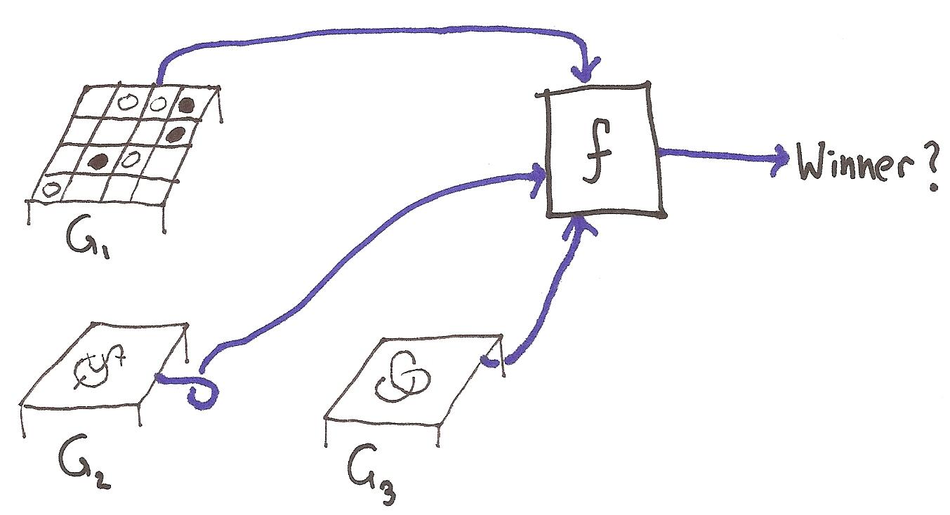
Figure 10.1: Schematically, we are playing several games in parallel and using $f$ to combine their final scores.

Algebraic properties of $f$ often lift to algebraic properties of $\tilde{f}$. For example, since addition of integers is associative and commutative, so is addition of games. Or if $f,g$, and $h$ are functions from $\mathbb{Z}$ to $\mathbb{Z}$, then $f\circ g=h\implies\tilde{f}\circ\tilde{g}=\tilde{h}$. Similar results hold for compositions of functions of higher arities. We will use these facts without comment in what follows.

Exercise 10.1.2.

Show than an algebraic identity will be maintained as long as each variable occurs exactly once on each side. So associativity and commutativity are maintained.

On the other hand, properties like idempotence and distributivity are not preserved, because even structurally, $\tilde{f}(G,G)$ is very different than $G$, having many more positions. In fact if $G$ is odd-tempered, then $\tilde{f}(G,G)$ will be even-tempered and so cannot equal or even be equivalent to $G$.

We are mainly interested in cases where $f$ has the following property:

Definition 10.1.3.

We say that $f~{}S_{1}\times\cdots\times S_{k}\to T$ is (weakly) order-preserving if whenever $(a_{1},\ldots,a_{n})\in S_{1}\times\cdots\times S_{k}$ and $(b_{1},\ldots,b_{n})\in S_{1}\times\cdots\times S_{k}$ satisfy $a_{i}\leq b_{i}$ for every $1\leq i\leq k$, then $f(a_{1},\ldots,a_{n})\leq f(b_{1},\ldots,b_{n})$.

Order-preserving operations are closed under composition. Moreover, unary order-preserving functions have the following nice property, which will be used later:

Lemma 10.1.4.

If $S,T$ are subsets of $\mathbb{Z}$, and $f:S\to T$ is order-preserving, then for any $G\in\mathcal{W}_{S}$,

$$\operatorname{R}(\tilde{f}(G))=f(\operatorname{R}(G)),$$

and

$$\operatorname{L}(\tilde{f}(G))=f(\operatorname{L}(G))$$

Proof.

Easy by induction; left as an exercise to the reader. ∎

We also have

Lemma 10.1.5.

Let $f$ and $g$ be two functions from $S_{1}\times\cdots\times S_{k}\to T$, such that $f(x_{1},\ldots,x_{k})\leq g(x_{1},\ldots,x_{k})$ for every $(x_{1},\ldots,x_{k})\in S_{1}\times\cdots\times S_{k}$. Then for every $(G_{1},\ldots,G_{k})\in\mathcal{W}_{S_{1}}\times\cdots\times\mathcal{W}_{S_{k}}$,

$$\tilde{f}(G_{1},\ldots,G_{k})\lesssim\tilde{g}(G_{1},\ldots,G_{k})$$

and in particular

$$\operatorname{o^{\#}}(\tilde{f}(G_{1},\ldots,G_{k}))\leq\operatorname{o^{\#}}(\tilde{g}(G_{1},\ldots,G_{k}))$$

Proof.

An obvious inductive proof using Theorem 9.4.4. ∎

Another easy fact is the following:

Lemma 10.1.6.

Let $f:S_{1}\times\cdots\times S_{k}\to T$ be a function. Then for any games $(G_{1},G_{2},\ldots,G_{k})\in\mathcal{W}_{S_{1}}\times\cdots\times\mathcal{W}_{S_{k}}$, we have

$$f(G_{1}+*,G_{2},\ldots,G_{k})=f(G_{1},G_{2}+*,\ldots,G_{k})=\cdots=$$

$$f(G_{1},G_{2},\ldots,G_{k}+*)=f(G_{1},\ldots,G_{k})+*,$$ (10.1)

where $*$ is $\langle 0|0\rangle$ as usual.

Proof.

Note that for $(x_{1},\ldots,x_{k},y)\in S_{1}\times\cdots\times S_{k}\times\{0\}$,

$$f(x_{1}+y,x_{2},\ldots,x_{k})=f(x_{1},x_{2}+y,\ldots,x_{k})=\cdots=$$

$$f(x_{1},x_{2},\ldots,x_{k}+y)=f(x_{1},\ldots,x_{k})+y.$$

It follows that (10.1) is true more generally if we replace $*$ by any $\{0\}$-valued game. ∎

10.2 Compatibility with Equivalence

We defined $\approx$ to be indistinguishability for the operation of addition. By adding new operations into the mix, indistinguishability could conceivably become a finer relation. In this section, we’ll see that this does not occur when our operations are extensions of order-preserving functions. In other words, the $\approx$ equivalence relation is already compatible with extensions of order-preserving functions.

Theorem 10.2.1.

Let $S_{1},\ldots,S_{k},T$ be subsets of $\mathbb{Z}$, $f:S_{1}\times\cdots\times S_{k}\to T$ be order-preserving, and $\tilde{f}$ be its extension to $\mathcal{W}_{S_{1}}\times\cdots\times\mathcal{W}_{S_{k}}\to\mathcal{W}_{T}$. Let $\Box$ be one of $\lesssim$, $\gtrsim$, $\lesssim_{\pm}$, $\gtrsim_{\pm}$, $\approx$, or $\approx_{\pm}$. If $(G_{1},\ldots,G_{k})$ and $(H_{1},\ldots,H_{k})$ are elements of $\mathcal{W}_{S_{1}}\times\cdots\mathcal{W}_{S_{k}}$, such that $G_{i}\Box H_{i}$ as integer-valued games, then

$$\tilde{f}(G_{1},\ldots,G_{k})\Box\tilde{f}(H_{1},\ldots,H_{k}).$$

This theorem says that extensions of order-preserving maps are compatible with equivalence and all our other relations. In particular, order-preserving extensions are well-defined on the quotient spaces of $\approx$ and $\approx_{\pm}$.

To prove Theorem 10.2.1, we reduce to the case where $G_{i}=H_{i}$ for all but one $i$, by the usual means. By symmetry, we only need to show that $\tilde{f}(G,G_{2},\ldots,G_{k})\lesssim_{-}\tilde{f}(H,G_{2},\ldots,G_{k})$, when $G\lesssim_{-}H$. We also reduce to the case where the codomain $T$ is $\{0,1\}$. This makes $T^{S_{1}}$, the set of order-preserving functions from $S_{1}$ to $T$ be itself finite and linearly ordered. We then view $f(\cdot,G_{2},\ldots,G_{k})$, the context into which $G$ and $H$ are placed, as a $T^{S_{1}}$-valued game whose score is combined with the final score of $G$ or $H$. (See Figure 10.2).

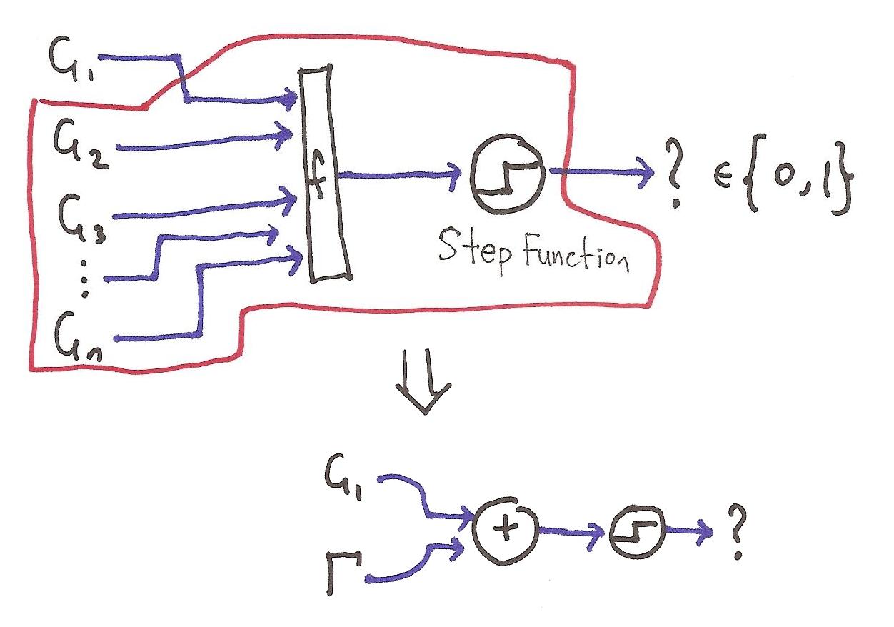
Figure 10.2: Schematically, we are taking all the component games other than $G$, as well as the function $f$, and bundling them up into a “context” $\Gamma$. In order to pull this off, we have to run the output of the game through a step function. By varying the cutoff of the step function, the true outcome of $\tilde{f}(G_{1},\ldots,G_{n})$ is recoverable, so this is no great loss.

As a finite total order, $T^{S_{1}}$ can then be identified with a set of integers slightly larger than $S_{1}$, and applying this identification to $f(\cdot,G_{2},\ldots,G_{k})$, we make an integer-valued game $A$ such that

$$\operatorname{o^{\#}}(G+A)\leq\operatorname{o^{\#}}(H+A)\implies\operatorname{o^{\#}}(G,G_{2},\ldots,G_{k})\leq\operatorname{o^{\#}}(H,G_{2},\ldots,G_{k}).$$

Many of these steps will not be spelled out explicitly in what follows.

Lemma 10.2.2.

Let $S,S_{2},\ldots,S_{k+1}$ be subsets of the integers, with $S$ finite, and let $f^{\prime}:S\times S_{2}\times\cdots\times S_{k+1}\to\mathbb{Z}$ be order-preserving. Then for any $n\in\mathbb{Z}$, there is a function $g_{n}:S_{2}\times\cdots\times S_{k+1}\to\mathbb{Z}$, such that for any $(x_{1},\ldots,x_{k+1})\in S\times S_{2}\times\ldots S_{k+1}$,

$$x_{1}+g_{n}(x_{2},x_{3},\ldots,x_{k+1})>0\iff f^{\prime}(x_{1},x_{2},\ldots,x_{k+1})>n.$$ (10.2)

(Note that there is no stipulation that $g_{n}$ be order-preserving.)

Proof.

Fix $x_{2},x_{3},\ldots,x_{k+1}$. Partition $S$ as $A\cup B$, where

$$A=\{x\in S~{}:~{}f^{\prime}(x,x_{2},\ldots,x_{k+1})>n\}$$

$$B=\{x\in S~{}:~{}f^{\prime}(x,x_{2},\ldots,x_{k+1})\leq n\}$$

Then because $f^{\prime}$ is order-preserving, every element of $A$ is greater than every element of $B$. Since $S$ is finite, this implies that there is some integer $m$ such that $A=\{x\in S:x>m\}$ and $B=\{x\in S:x\leq m\}$. Let $g_{n}(x_{2},\ldots,x_{k+1})=-m$. Then clearly (10.2) will hold. ∎

Lemma 10.2.3.

With the setup of the previous lemma, if $G$ is an $S$-valued game, and $G_{i}$ is a $S_{i}$-valued game for $2\leq i\leq k+1$, then

$$\operatorname{L}(G+\tilde{g}(G_{2},\ldots,G_{k+1}))>0\iff\operatorname{L}(\tilde{f^{\prime}}(G,G_{2},\ldots,G_{k+1}))>n$$

and similarly

$$\operatorname{R}(G+\tilde{g}(G_{2},\ldots,G_{k+1}))>0\iff\operatorname{R}(\tilde{f^{\prime}}(G,G_{2},\ldots,G_{k+1}))>n$$

Proof.

For any integer $m$, let $\delta_{m}~{}:~{}\mathbb{Z}\to\{0,1\}$ be the function $\delta_{m}(x)=1$ if $x>m$ and $\delta_{m}(x)=0$ if $x\leq m$. Then using Lemma 10.1.4, we have

$$\operatorname{L}(G+\tilde{g_{n}}(G_{2},\ldots,G_{k+1}))>0\iff\operatorname{L}(\tilde{\delta_{0}}(G+\tilde{g_{n}}(G_{2},\ldots,G_{k+1})))=1,$$ (10.3)

and similarly,

$$\operatorname{L}(\tilde{f^{\prime}}(G,G_{2},\ldots,G_{k+1}))>n\iff\operatorname{L}(\tilde{\delta_{n}}(\tilde{f^{\prime}}(G,G_{2},\ldots,G_{k+1})))=1.$$ (10.4)

Now by the previous lemma, we know that for any $(x_{1},\ldots,x_{k+1})\in S\times S_{2}\times\cdots\times S_{k+1}$, we have

$$\delta_{0}(x_{1}+g_{n}(x_{2},x_{3},\ldots,x_{k}))=\delta_{n}(x_{1},x_{2},\ldots,x_{k})$$

But then this equation continues to be true when we extend everything to games, so that

$$\tilde{\delta_{0}}(G+\tilde{g_{n}}(G_{2},\ldots,G_{k+1}))=\tilde{\delta_{n}}(\tilde{f^{\prime}}(G,G_{2},\ldots,G_{k+1}))$$

and then we are done, after combining with (10.3) and (10.4) above. ∎

Now since $G+\tilde{g_{n}}(G_{2},\ldots,G_{k})$ has the same parity as $\tilde{f}(G,G_{2},\ldots,G_{k})$, the two equations in Lemma 10.2.3 are equivalent to the following two:

$$\operatorname{Lf}(G+\tilde{g_{n}}(G_{2},\ldots,G_{k}))>0\iff\operatorname{Lf}(\tilde{f}(G,G_{2},\ldots,G_{k}))>n$$ (10.5)

$$\operatorname{Rf}(G+\tilde{g_{n}}(G_{2},\ldots,G_{k}))>0\iff\operatorname{Rf}(\tilde{f}(G,G_{2},\ldots,G_{k}))>n$$ (10.6)

Lemma 10.2.4.

If $(G_{1},\ldots,G_{k})$ and $(H_{1},\ldots,H_{k})$ are in $\mathcal{W}_{S_{1}}\times\mathcal{W}_{S_{2}}\times\cdots\times\mathcal{W}_{S_{k}}$, and $G_{i}\lesssim_{-}H_{i}$ for every $i$, and $G_{i}=H_{i}$ for all but one $i$, then

$$\tilde{f}(G_{1},\ldots,G_{k})\lesssim_{-}\tilde{f}(H_{1},\ldots,H_{k}).$$

Also, the same holds if we replace $\lesssim_{-}$ with $\lesssim_{+}$.

Proof.

Without loss of generality, $G_{i}=H_{i}$ for all $i\neq 1$. We only need to consider the case where $G_{1}\lesssim_{-}H_{1}$, as the $G_{1}\lesssim_{+}H_{1}$ case follows by symmetry.

We want to show that

$$\tilde{f}(G,G_{2},\ldots,G_{k})\lesssim_{-}\tilde{f}(H,G_{2},\ldots,G_{k})$$

given that $G\lesssim_{-}H$ are $S_{1}$-valued games. In particular, we need to show that for every game $K$,

$$\operatorname{Lf}(\tilde{f}(G,G_{2},\ldots,G_{k})+K)\leq\operatorname{Lf}(\tilde{f}(H,G_{2},\ldots,G_{k})+K).$$ (10.7)

Suppose for the sake of contradiction that there is some $K$ for which (10.7) doesn’t hold. Then there is some integer $n$ such that

$$\operatorname{Lf}(\tilde{f}(H,G_{2},\ldots,G_{k})+K)\not>n$$

but

$$\operatorname{Lf}(\tilde{f}(G,G_{2},\ldots,G_{k})+K)>n.$$

Let $S_{k+1}$ be $\mathbb{Z}$, so that $K$ is an $S_{k+1}$-valued game. Since all our games are finite, only finitely many values occur within each of $G$ and $H$. Thus there is some finite subset $S$ of $S_{1}$ so that $G$ and $H$ are both $S$-valued games. Let $f^{\prime}~{}:~{}S\times S_{1}\times\cdots\times S_{k}\times S_{k+1}$ be the function

$$f^{\prime}(x_{1},\ldots,x_{k+1})=f(x_{1},\ldots,x_{k})+x_{k+1},$$

which is still order-preserving. Then $\tilde{f^{\prime}}(G_{1},\ldots,G_{k+1})=\tilde{f}(G_{1},\ldots,G_{k})+G_{k+1}$ for any appropriate $G_{1},\ldots,G_{k+1}$. In particular, then, we have that

$$\operatorname{Lf}(\tilde{f^{\prime}}(H,G_{2},\ldots,G_{k},K))\not>n$$

and

$$\operatorname{Lf}(\tilde{f^{\prime}}(G,G_{2},\ldots,G_{k},K))>n$$

Let $g_{n}$ be the function from Lemma 10.2.3. Then by (10.5), it follows that

$$\operatorname{Lf}(H+\tilde{g_{n}}(G_{2},\ldots,G_{k},K))\not>0$$

and

$$\operatorname{Lf}(G+\tilde{g_{n}}(G_{2},\ldots,G_{k},K))>0.$$

Thus, if $J=\tilde{g_{n}}(G_{2},\ldots,G_{k},K)$, we have $\operatorname{Lf}(G+J)\not\leq\operatorname{Lf}(H+J)$, contradicting the fact that $G\lesssim_{-}H$.

The other case, in which $G\lesssim_{+}H$, follows by symmetry. ∎

Proof (of Theorem 10.2.1).

With the setup of Theorem 10.2.1, first consider the case where $\Box$ is $\lesssim_{-}$. So $G_{i}\lesssim_{-}H_{i}$ for every $i$. Then by Lemma 10.2.4,

$$\tilde{f}(G_{1},\ldots,G_{k})\lesssim_{-}\tilde{f}(H_{1},G_{2}\ldots,G_{k})\lesssim_{-}\tilde{f}(H_{1},H_{2},G_{3},\ldots,G_{k})$$

$$\lesssim_{-}\cdots\lesssim_{-}\tilde{f}(H_{1},\ldots,H_{k-1},G_{k})\lesssim_{-}\tilde{f}(H_{1},\ldots,H_{k}).$$

So $\tilde{f}(G_{1},\ldots,G_{k})\lesssim_{-}\tilde{f}(H_{1},\ldots,H_{k})$ by transitivity of $\lesssim_{-}$. This establishes Theorem 10.2.1 when $\Box$ is $\lesssim_{-}$.

The cases where $\Box$ is one of $\lesssim_{+}$, $\gtrsim_{+}$ or $\gtrsim_{-}$ follow immediately. All the other remaining possibilities for $\Box$ can be written as intersections of $\lesssim_{\pm}$ and $\gtrsim_{\pm}$, so the remaining cases follow easily. For example, if $G_{i}\approx_{+}H_{i}$ for all $i$, then we have $G_{i}\lesssim_{+}H_{i}$ and $G_{i}\gtrsim_{+}H_{i}$ for all $i$, so that

$$\tilde{f}(G_{1},\ldots,G_{k})\lesssim_{+}\tilde{f}(H_{1},\ldots,H_{k})$$

and

$$\tilde{f}(G_{1},\ldots,G_{k})\gtrsim_{+}\tilde{f}(H_{1},\ldots,H_{k})$$

by the cases where $\Box$ is $\lesssim_{+}$ or $\gtrsim_{+}$. Thus

$$\tilde{f}(G_{1},\ldots,G_{k})\approx_{+}\tilde{f}(H_{1},\ldots,H_{k}).$$

∎

As a corollary of Theorem 10.2.1, we see that the action of an order-preserving extension on $S$-valued games is determined by its action on even-tempered i-games.

Corollary 10.2.5.

Let $S_{1},S_{2},\ldots,S_{k},T$ be subsets of $\mathbb{Z}$, and $f:S_{1}\times\cdots\times S_{k}\to T$ be order-preserving. For $1\leq i\leq k$, let $G_{i}$ be an $S_{i}$-valued game. Let $e_{i}$ be $0$ or $*$, so that $e_{i}$ has the same parity as $G_{i}$. For each $G_{i}$, choose an upside and downside $G_{i}^{+}$ and $G_{i}^{-}$ which are $S_{i}$-valued, possible by Theorem 9.5.2(g). Then for every $i$, $G_{i}^{+}+e_{i}$ and $G_{i}^{-}+e_{i}$ are even-tempered $S_{i}$-valued i-games, and

$$\tilde{f}(G_{1},\ldots,G_{k})\approx A\&B+(e_{1}+\cdots+e_{k}),$$

where

$$A\approx\tilde{f}(G_{1}^{+}+e_{1},G_{2}^{+}+e_{2},\ldots,G_{k}^{+}+e_{k})^{+}$$

$$B\approx\tilde{f}(G_{1}^{-}+e_{2},G_{2}^{-}+e_{2},\ldots,G_{k}^{-}+e_{k})^{-}$$

are even-tempered i-games.

Proof.

First consider the case where every $G_{i}$ is even-tempered, so that all the $e_{i}$ vanish. Then we need to show that

$$\tilde{f}(G_{1},\ldots,G_{k})^{+}\approx A$$

$$\tilde{f}(G_{1},\ldots,G_{k})^{-}\approx B$$

or equivalently,

$$\tilde{f}(G_{1},\ldots,G_{k})\approx_{+}\tilde{f}(G_{1}^{+},G_{2}^{+},\ldots,G_{k}^{+})$$

$$\tilde{f}(G_{1},\ldots,G_{k})\approx_{-}\tilde{f}(G_{1}^{-},G_{2}^{-},\ldots,G_{k}^{-}).$$

But these follow directly from Theorem 10.2.1 in the case where $\Box$ is $\approx_{\pm}$, since $G_{i}\approx_{\pm}G_{i}^{\pm}$ for all $i$.

Now suppose that some of the $G_{i}$ are odd-tempered. Since $*$ is an i-game, every $G_{i}^{\pm}+e_{i}$ is an i-game too, and is $S_{i}$-valued because $G_{i}^{\pm}$ is $S_{i}$-valued and $e_{i}$ is $\{0\}$-valued. Now $G_{i}$, $G_{i}^{\pm}$, and $e_{i}$ all have the same parity, so $G_{i}^{\pm}+e_{i}$ will be even-tempered $S_{i}$-valued i-games.

Letting $H_{i}=G_{i}+e_{i}$, we see that $H_{i}$ is an even-tempered $S_{i}$-valued game for every $i$, and that $H_{i}^{\pm}\approx G_{i}^{\pm}+e_{i}$ because $e_{i}$ is an i-game. Now $0+0=0$, and $*+*\approx 0$ (as $*$ equals its own negative), so $G_{i}\approx H_{i}+e_{i}$ for every $i$. Then by Theorem 10.2.1 and repeated applications of Lemma 10.1.6, we see that

$$\tilde{f}(G_{1},\ldots,G_{k})\approx\tilde{f}(H_{1}+e_{1},\ldots,H_{k}+e_{k})=\tilde{f}(H_{1},\ldots,H_{k})+(e_{1}+\cdots+e_{k}).$$

But by the even-tempered case that we just proved,

$$\tilde{f}(H_{1},\ldots,H_{k})\approx A\&B.$$

∎

10.3 Preservation of i-games

By Corollary 10.2.5, any order-preserving extension $\tilde{f}$ is determined by two maps on even-tempered i-games, one that sends

$$(G_{1},\ldots,G_{k})\to\tilde{f}(G_{1},\ldots,G_{k})^{+}$$

and one that sends

$$(G_{1},\ldots,G_{k})\to\tilde{f}(G_{1},\ldots,G_{k})^{-}.$$

In this section we show that in fact $\tilde{f}(G_{1},\ldots,G_{k})$ will always be an i-game itself, so that these two maps in fact agree. Thus every order-preserving map $f$ induces a single map on equivalence classes of even-tempered i-games, and this map determines the action of $f$ on all games.

We first prove that i-games are preserved for the case where $f$ is unary, and use it to answer a question from a previous chapter: for which $A\gtrsim B$ does $A\&B$ exist?

Lemma 10.3.1.

Let $S$ be a set of integers, and $f:S\to\mathbb{Z}$ be weakly order-preserving. Then for any $S$-valued i-game $G$, $\tilde{f}(G)$ is an i-game.

Proof.

By induction, we only need to show that if $G$ is even-tempered, then

$$\operatorname{L}(\tilde{f}(G))\geq\operatorname{R}(\tilde{f}(G)),$$

which follows by Lemma 10.1.4 and the fact that $\operatorname{L}(G)\geq\operatorname{R}(G)$. ∎

Lemma 10.3.2.

If $G$ is an $S$-valued game and $f:S\to\mathbb{Z}$ is order-preserving, then

$$\tilde{f}(G)^{+}\approx\tilde{f}(G^{+})$$

$$\tilde{f}(G)^{-}\approx\tilde{f}(G^{-})$$

where we take $G^{\pm}$ to be $S$-valued.

Proof.

We have $G^{\pm}\approx_{\pm}G$, so by Theorem 10.2.1,

$$\tilde{f}(G)\approx_{\pm}\tilde{f}(G^{\pm}).$$

But by Lemma 10.3.1, $\tilde{f}(G^{\pm})$ is an i-game because $G^{\pm}$ is. So the desired result follows. ∎

We now complete the description of $\mathcal{W}_{\mathbb{Z}}$ in terms of i-games:

Lemma 10.3.3.

If $A$ is an i-game (necessarily even-tempered) with $A\gtrsim 0$, then there is some $\mathbb{Z}$-valued game $H$ with $H^{-}\approx 0$ and $H^{+}\approx A$.

Proof.

For any integers $n\leq m$, let $D_{n,m}$ denote the even-tempered game $\langle n+*\,|\,m+*\rangle$. The reader can verify from the definitions that $D_{n,m}^{+}=m$ and $D_{n,m}^{-}=n$, so that $D_{n,m}$ acts like either $n$ or $m$ depending on its context.

We create $H$ from $A$ by substituting $D_{0,n}$ for every positive number $n$ occurring within $A$. As $D_{0,n}^{+}=n$, it follows by an inductive argument using the $\approx_{+}$ case of Theorem 9.4.4 that $A$ is still the upside of $H$.

It is also clear by the $\approx_{-}$ case of Theorem 9.4.4 that the downside of $H$ is the downside of the game obtained by replacing every positive number in $A$ with $0$. Letting $f(n)=\min(n,0)$, this game is just $\tilde{f}(A)$. So $H^{-}\approx f(A)^{-}$. But $A\approx_{-}A^{-}$, so by Theorem 10.2.1 $f(A)\approx_{-}f(A^{-})$. Then by Lemma 10.3.1, $f(A^{-})$ is an i-game, so $f(A)^{-}\approx f(A^{-})$. Thus

$$H^{-}\approx f(A)^{-}\approx f(A^{-})\approx f(A).$$

Moreover, since $A\gtrsim 0$, Corollary 9.3.2 implies that $\operatorname{R}(A)\geq 0$. As an even-tempered i-game, $\operatorname{L}(A)\geq\operatorname{R}(A)\geq 0$. Therefore $f(\operatorname{L}(A))=f(\operatorname{R}(A))=0$. By Lemma 10.1.4, it then follows that $\operatorname{L}(f(A))=\operatorname{R}(f(A))=0$. Then by Corollary 9.3.2, $f(A)\approx 0$, so $H^{-}\approx 0$ and we are done. ∎

Using this, we see that all possible pairs $A\&B$ occur:

Theorem 10.3.4.

If $A$, $B$ are i-games with $A\gtrsim B$, then there is some $\mathbb{Z}$-valued game $G$ with $G^{+}\approx A$ and $G^{-}\approx B$.

Proof.

Since $A-B\gtrsim 0$, we can produce a game $H$ with $H^{+}\approx A-B$ and $H^{-}\approx 0$ by the lemma. Then letting $G=H+B$, we have

$$G^{+}\approx H^{+}+B^{+}\approx A-B+B\approx A,$$

$$G^{-}\approx H^{-}+B^{-}\approx 0+B=B.$$

∎

Moreover, we can refine this slightly:

Theorem 10.3.5.

Let $\mathcal{S}\subseteq\mathbb{Z}$ and let $A$ and $B$ be $\mathcal{S}$-valued i-games with $A\gtrsim B$. Then there is some $\mathcal{S}$-valued game $G$ with $G^{+}\approx A$ and $G^{-}\approx B$.

Proof.

By the previous theorem, we can construct a game $G_{0}$ with $G_{0}^{+}\approx A$ and $G_{0}^{-}\approx B$. Let $f\,:\,\mathbb{Z}\to\mathbb{Z}$ be a weakly order-preserving function that projects $\mathbb{Z}$ onto $\mathcal{S}$. That is, $f\circ f=f$, and $f(\mathbb{Z})=\mathcal{S}$. We can construct such an $f$ by sending every integer to the closest element of $\mathcal{S}$, breaking ties arbitrarily. (Note that by existence of $A$ and $B$, $\mathcal{S}$ cannot be empty.) Then by Lemma 10.3.2 and Theorem 10.2.1,

$$f(G_{0})^{+}\approx f(G_{0}^{+})\approx f(A)=A$$

and

$$f(G_{0})^{-}\approx f(G_{0}^{-})\approx f(B)=B,$$

so taking $G=f(G_{0})$, we have $G\in\mathcal{W}_{\mathcal{S}}$, and $G^{+}\approx A$ and $G^{-}\approx B$. ∎

So for any $\mathcal{S}\subseteq\mathbb{Z}$, the $\mathcal{S}$-valued games modulo $\approx$ are in one-to-one correspondence with the pairs $(a,b)\in\mathcal{I}_{\mathcal{S}}\times\mathcal{I}_{\mathcal{S}}$ for which $a\gtrsim b$, where $\mathcal{I}_{\mathcal{S}}$ is the $\mathcal{S}$-valued i-games modulo $\approx$. In particular, $A\&B$ exists and can be $S$-valued whenever $A$ and $B$ are $S$-valued i-games with $A\gtrsim B$.

We now return to proving that order-preserving extensions preserve i-games:

Theorem 10.3.6.

Let $S_{1},\ldots,S_{k},T$ be subsets of $\mathbb{Z}$, $f:S_{1}\times\cdots\times S_{k}\to T$ be order-preserving, and $\tilde{f}$ be the extension of $f$ to $\mathcal{W}_{S_{1}}\times\cdots\times\mathcal{W}_{S_{k}}\to\mathcal{W}_{T}$. If $G_{1},\ldots,G_{k}$ are i-games, with $G_{i}\in\mathcal{W}_{S_{i}}$, then $\tilde{f}(G_{1},\ldots,G_{k})$ is also an i-game. Moreover, if $H_{1},\ldots,H_{k}$ are general games, with $H_{i}\in\mathcal{W}_{S_{i}}$, then

$$(\tilde{f}(H_{1},\ldots,H_{k}))^{+}\approx\tilde{f}(H_{1}^{+},H_{2}^{+},\ldots,H_{k}^{+})$$

and

$$(\tilde{f}(H_{1},\ldots,H_{k}))^{-}\approx\tilde{f}(H_{1}^{-},H_{2}^{-},\ldots,H_{k}^{-}).$$

In other words, $f$ preserves i-games, and interacts nicely with upsides and downsides.

Proof.

The first claim is the more difficult to show. It generalizes Theorem 9.2.11 and Lemma 10.3.1. We first prove a slightly weaker form:

Lemma 10.3.7.

If $(G_{1},\ldots,G_{k})\in\mathcal{W}_{S_{1}}\times\cdots\times\mathcal{W}_{S_{k}}$ are all i-games, then $\tilde{f}(G_{1},\ldots,G_{k})\approx H$ for some i-game $H\in\mathcal{W}_{\mathbb{Z}}$.

Proof.

Since each $G_{i}$ is finite, it has only finitely many elements of $S_{i}$ as subpositions - so we can take finite subsets $S^{\prime}_{i}\subseteq S_{i}$ such that $G_{i}\in\mathcal{W}_{S_{i}^{\prime}}$ for every $i$. Restricting $f$ from $S_{i}$ to $S^{\prime}_{i}$, we can assume without loss of generality that $S_{i}=S_{i}^{\prime}$ is finite. Then there is some positive integer $M$ so that

$$|f(x_{1},\ldots,x_{k})|<\frac{M}{2}$$

for every $(x_{1},\ldots,x_{k})\in S_{1}\times\cdots\times S_{k}$.

For each $i$, let $Z_{i}=\{-s\,:\,s\in S\}$ and let $g:~{}Z_{1}\times\cdots\times Z_{k}\to\mathbb{Z}$ be the order preserving function

$$g(x_{1},\ldots,x_{k})=-f(-x_{1},\ldots,-x_{k}).$$

I claim that

$$\tilde{f}(G_{1},\ldots,G_{k})+\tilde{g}(-G_{1},-G_{2},\ldots,-G_{k})\approx 0$$ (10.8)

so that $\tilde{f}(G_{1},\ldots,G_{k})\approx$ an i-game by Theorem 9.5.2(f). To show (10.8) we need to show that for any integer-valued game $K$,

$$\operatorname{o^{\#}}(\tilde{f}(G_{1},\ldots,G_{k})+\tilde{g}(-G_{1},\ldots,-G_{k})+K)=\operatorname{o^{\#}}(K).$$ (10.9)

We show that the left hand side is $\geq$ than the right hand side by essentially showing that Left can play the sum $G_{1}+\cdots+G_{k}+(-G_{1})+\cdots+(-G_{k})+K$ in such a way that her score in each $G_{i}$ component outweighs the score in the corresponding $-G_{i}$ component. The other direction of the inequality follows by symmetry.

First of all, notice that since the $G_{i}$ are i-games by assumption, $G_{i}-G_{i}\approx 0$ for every $i$ and so

$$\operatorname{o^{\#}}((G_{1}-G_{1})+\cdots+(G_{k}-G_{k})+K)=\operatorname{o^{\#}}(K).$$

Now we distort this sum by putting exorbitant penalties on Left for failing to ensure that the final score of any of the $G_{i}-G_{i}$ components is $\geq 0$. Specifically, let $\delta:~{}\mathbb{Z}\to\mathbb{Z}$ be the function given by $\delta(x)=0$ if $x\geq 0$, and $\delta(x)=-M$ if $x<0$. Then by Lemma 10.3.1 $\delta(G_{i}-G_{i})$ is an i-game because $G_{i}-G_{i}$ is. Moreover, $\delta(G_{i}-G_{i})$ must have outcomes $(\delta(0),\delta(0))=(0,0)$, so that by Lemma 9.4.8 $\delta(G_{i}-G_{i})\approx 0$. Therefore,

$$\operatorname{o^{\#}}(\delta(G_{1}-G_{1})+\cdots+\delta(G_{k}-G_{k})+K)=\operatorname{o^{\#}}(K).$$ (10.10)

Now let $h_{1}$ and $h_{2}$ be functions $S_{1}\times\cdots\times S_{k}\times Z_{1}\times\cdots\times Z_{k}\times\mathbb{Z}\to\mathbb{Z}$ given by

$$h_{1}(x_{1},\ldots,x_{k},y_{1},\ldots,y_{k},z)=\delta(x_{1}+y_{1})+\delta(x_{2}+y_{2})+\cdots+\delta(x_{k}+y_{k})+z$$

and

$$h_{2}(x_{1},\ldots,x_{k},y_{1},\ldots,y_{k},z)=f(x_{1},\ldots,x_{k})+g(y_{1},\ldots,y_{k})+z$$

Then we can write (10.10) as

$$\operatorname{o^{\#}}(\tilde{h_{1}}(G_{1},\ldots,G_{k},-G_{1},\ldots,-G_{k},K))=\operatorname{o^{\#}}(K).$$

Suppose we know that $h_{1}\leq h_{2}$ for all possible inputs. Then Lemma 10.1.5 implies that

$$\operatorname{o^{\#}}(\tilde{h_{2}}(G_{1},\ldots,G_{k},-G_{1},\ldots,-G_{k},K))\geq\operatorname{o^{\#}}(K)$$

which is just the $\geq$ direction of (10.9). By symmetry the $\leq$ direction of (10.9) also follows and we are done. So it remains to show that $h_{1}\leq h_{2}$, i.e.,

$$\delta(x_{1}+y_{1})+\cdots+\delta(x_{k}+y_{k})\leq f(x_{1},\ldots,x_{k})+g(y_{1},\ldots,y_{k})$$ (10.11)

for all $(x_{1},\ldots,x_{k},y_{1},\ldots,y_{k})\in S_{1}\times\cdots\times S_{k}\times Z_{1}\times\cdots\times Z_{k}$.

Suppose first that $x_{i}+y_{i}\geq 0$ for all $i$. Then $\delta(x_{i}+y_{i})=0$ for all $i$ so the left hand side of (10.11) is zero. On the other hand, since $-y_{i}\leq x_{i}$ for every $i$, and $f$ is order preserving,

$$-g(y_{1},\ldots,y_{k})=f(-y_{1},\ldots,-y_{k})\leq f(x_{1},\ldots,x_{k}),$$

so (10.11) holds. Otherwise, $x_{i}+y_{i}<0$ for some $i$, and so the left hand side of (10.11) is $\leq-M$. On the other hand, the right hand side is at least $-M$, by choice of $M$ (and the fact that the range of $g$ is also bounded between $-M$ and $M$). Therefore (10.11) again holds, and we are done. ∎

Now the Lemma shows that $\tilde{f}(G_{1},\ldots,G_{k})$ is equivalent to an i-game. We can easily use this to show that it is in fact an i-game. Note that every subposition of $\tilde{f}(G_{1},\ldots,G_{k})$ is of the form $\tilde{f}(G_{1}^{\prime},\ldots,G_{k}^{\prime})$ where $G_{i}^{\prime}$ is a subposition of $G_{i}$ for every $i$. By definition of i-game, the $G_{i}^{\prime}$ will also be equivalent to i-games, and so by the previous lemma every subposition of $\tilde{f}(G_{1},\ldots,G_{k})$ is equivalent to an i-game. So by the following lemma, $\tilde{f}(G_{1},\ldots,G_{k})$ is itself an i-game:

Lemma 10.3.8.

If $G$ is an integer-valued game, and every subposition of $G$ is equivalent ($\approx$) to an i-game, then $G$ is an i-game.

Proof.

$G$ is an i-game as long as every even-tempered subposition $G^{\prime}$ satisfies $\operatorname{L}(G^{\prime})\geq\operatorname{R}(G^{\prime})$. But if $G^{\prime}$ is an even-tempered subposition of $G$, then $G$ equals an i-game $H$ by assumption, and $H$ is even-tempered by Theorem 9.3.3. So $\operatorname{L}(H)\geq\operatorname{R}(H)$. But $G^{\prime}\approx H$ implies that $\operatorname{o^{\#}}(G^{\prime})=\operatorname{o^{\#}}(H)$. ∎

For the last claim of Theorem 10.3.6, let $H_{1},\ldots,H_{k}$ be general games with $H_{i}\in\mathcal{W}_{S_{i}}$. Then $H_{i}\lesssim_{+}H_{i}^{+}$ and $H_{i}^{+}\lesssim H_{i}$ for every $i$, so by Theorem 10.2.1,

$$\tilde{f}(H_{1},\ldots,H_{k})\lesssim_{+}\tilde{f}(H_{1}^{+},\ldots,H_{k}+)$$

and

$$\tilde{f}(H_{1}^{+},\ldots,H_{k}^{+})\lesssim_{+}\tilde{f}(H_{1},\ldots,H_{k})$$

so

$$\tilde{f}(H_{1},\ldots,H_{k})\approx_{+}\tilde{f}(H_{1}^{+},\ldots,H_{k}^{+}).$$

But we just showed that $\tilde{f}(H_{1}^{+},\ldots,H_{k}^{+})$ is equivalent to an i-game, so therefore

$$\tilde{f}(H_{1},\ldots,H_{k})^{+}\approx\tilde{f}(H_{1}^{+},\ldots,H_{k}^{+}).$$

The proof of the claim for downsides is completely analogous. This completes the proof of Theorem 10.3.6. ∎

Chapter 11 Reduction to Partizan theory

11.1 Cooling and Heating

The following definition is an imitation of the standard cooling and heating operators for partizan games, defined and discussed on pages 102-108 of ONAG and Chapter 6 of Winning Ways.

Theorem 11.1.1.

If $G$ is a $\mathbb{Z}$-valued game and $n$ is an integer (possibly negative), we define $G$ cooled by $n$, $G_{n}$, to be $G$ is $G$ is a number, and otherwise $\langle(G^{L})_{n}-n\,|\,(G^{R})_{n}+n\rangle$, where $G^{L}$ and $G^{R}$ range over the left and right options of $G$. We define $G$ heated by $n$ to be $G_{-n}$, $G$ cooled by $-n$.

The following results are easily verified from the definition:

Theorem 11.1.2.

Let $G$ and $H$ be games, and $n$ and $m$ be integers.

(a)

$(-G)_{n}=-(G_{n})$.

(b)

$(G+H)_{n}=G_{n}+H_{n}$.

(c)

If $G$ is even-tempered, then $\operatorname{L}(G_{n})=\operatorname{L}(G)$ and $\operatorname{R}(G_{n})=\operatorname{R}(G)$.

(d)

If $G$ is odd-tempered, then $\operatorname{L}(G_{n})=\operatorname{L}(G)-n$ and $\operatorname{R}(G_{n})=\operatorname{R}(G)+n$.

(e)

$(G_{n})_{m}=G_{n+m}$.

(f)

$G$ is an i-game iff $G_{n}$ is an i-game.

Note that there are no references to $\approx$.

Proof.

We proceed with inductive proofs in the style of ONAG. We mark the inductive step with $\stackrel{{\scriptstyle!}}{{=}}$.

$$(-G)_{n}=\langle(-G^{R})_{n}-n\,|\,(-G^{L})_{n}+n\rangle\stackrel{{\scriptstyle!}}{{=}}$$

$$\langle-(G^{R}_{n})-n|-(G^{L}_{n})+n\rangle=-\langle(G^{L})_{n}-n|(G^{R})_{n}+n\rangle=-(G_{n}),$$

unless $G$ is a number, in which case (a) is obvious.

$$(G+H)_{n}=\langle(G+H)^{L}_{n}-n|(G+H)^{R}_{n}+n\rangle=$$

$$\langle(G^{L}+H)_{n}-n,\,(G+H^{L})_{n}-n\,|\,(G^{R}+H)_{n}+n,\,(G+H^{R})_{n}+n\rangle\stackrel{{\scriptstyle!}}{{=}}$$

$$\langle G^{L}_{n}+H_{n}-n,\,G_{n}+H^{L}_{n}-n\,|\,G^{R}_{n}+H_{n}+n,\,G_{n}+H^{R}_{n}+n\rangle=G_{n}+H_{n},$$

unless $G$ and $H$ are both numbers, in which case (b) is obvious. If $G$ is even-tempered, then

$$\operatorname{L}(G_{n})=\max\{\operatorname{R}(G^{L}_{n}-n)\}\stackrel{{\scriptstyle!}}{{=}}\max\{\operatorname{R}(G^{L})+n-n\}=\max\{\operatorname{R}(G^{L})\}=\operatorname{L}(G),$$

unless $G$ is a number, in which case $\operatorname{L}(G_{n})=\operatorname{L}(G)$ is obvious. And similarly, $\operatorname{R}(G_{n})=\operatorname{R}(G)$. If $G$ is odd-tempered, then

$$\operatorname{L}(G_{n})=\max\{\operatorname{R}(G^{L}_{n}-n)\}\stackrel{{\scriptstyle!}}{{=}}\max\{\operatorname{R}(G^{L})-n\}=\operatorname{L}(G)-n,$$

and similarly $\operatorname{R}(G_{n})=\operatorname{R}(G)+n$.

$$(G_{n})_{m}=\langle(G_{n})^{L}_{m}-m\,|\,(G_{n})^{R}_{m}+m\rangle=\langle(G^{L}_{n}-n)_{m}-m\,|\,(G^{R}_{n}+n)_{m}+m\rangle\stackrel{{\scriptstyle*}}{{=}}$$

$$\langle(G^{L}_{n})_{m}-(n+m)\,|\,(G^{R}_{n})_{m}+(n+m)\rangle\stackrel{{\scriptstyle!}}{{=}}\langle G^{L}_{n+m}-(n+m)\,|\,G^{R}_{n+m}+(n+m)\rangle=G_{n+m},$$

unless $G$ is a number, in which case (e) is obvious. Here the $\stackrel{{\scriptstyle*}}{{=}}$ follows by part (b).

Finally, part (f) follows by an easy induction using part (c). ∎

Using these, we show that heating and cooling are meaningful modulo $\approx$ and $\approx_{\pm}$:

Theorem 11.1.3.

If $G$ and $H$ are games, $n\in\mathbb{Z}$, and $\Box$ is one of $\approx$, $\approx_{\pm}$, $\lesssim$, $\lesssim_{\pm}$, etc., then $G\ \Box\ H\iff G_{n}\ \Box\ H_{n}$.

Proof.

It’s enough to consider $\lesssim_{-}$ and $\lesssim_{+}$. By symmetry, we only consider $\lesssim_{-}$. By part (e) of the preceding theorem, cooling by $-n$ is exactly the inverse of cooling by $n$, so we only show that $G\lesssim_{-}H\Rightarrow G_{n}\lesssim_{-}H_{n}$. Let $G\lesssim_{-}H$. Then $G$ and $H$ have the same parity. Let $X$ be arbitrary. Note that $G_{n}+X$ and $H_{n}+X$ are just $(G+X_{-n})_{n}$ and $(H+X_{-n})$. By assumption, $\operatorname{Rf}(G+X_{-n})\leq\operatorname{Rf}(H+X_{-n})$, so by part (c) or (d) of the previous theorem (depending on the parities of $G,H,$ and $X$) we see that

$$\operatorname{Rf}(G_{n}+X)=\operatorname{Rf}((G+X_{-n})_{n})\leq\operatorname{Rf}((H+X_{-n})_{n})=\operatorname{Rf}(H_{n}+X).$$

Then since $X$ was arbitrary, we are done. ∎

So heating and cooling induce automorphisms of the commutative monoid $\mathcal{W}_{\mathbb{Z}}/\approx$ that we are interested in.

Definition 11.1.4.

For $n\in\mathbb{Z}$, let $I_{n}$ be recursively defined set of $\mathbb{Z}$-valued games such that $G\in I_{n}$ iff every option of $G$ is in $I_{n}$, and

• If $G$ is even-tempered, then $\operatorname{L}(G)\geq\operatorname{R}(G)$.

• If $G$ is odd-tempered, then $\operatorname{L}(G)-\operatorname{R}(G)\geq n$.

It’s clear that $I_{n}\subseteq I_{m}$ when $n>m$, and that the i-games are precisely the elements of $I=\bigcup_{n\in\mathbb{Z}}I_{n}$. Also, the elements of $\cap_{n\in\mathbb{Z}}I_{n}$ are nothing but the numbers, since any odd-tempered game fails to be in $I_{n}$ for some $n$.

The class $I_{0}$ consists of the games in which being unexpectedly forced to move is harmless. Just as looking at i-games allowed us to extends Equations (9.2-9.3) to other parities, the same thing happens here: if $G$ and $H$ are two games in $I_{0}$ with $\operatorname{R}(G)\geq 0$ and $\operatorname{R}(H)\geq 0$, then $\operatorname{R}(G+H)\geq 0$, regardless of parity. We have already seen this if $G$ and $H$ are even-tempered (Equation (9.2)) or if one of $G$ is odd-tempered (Equation (9.8)), and the final case, where both games are odd-tempered, comes from the following results:

Theorem 11.1.5.

Let $G$ and $H$ be $\mathbb{Z}$-valued games in $I_{n}$ for some $n$.

• If $G$ is odd-tempered and $H$ is odd-tempered, then

  $$\operatorname{R}(G+H)\geq\operatorname{R}(G)+\operatorname{R}(H)+n$$ (11.1)

• If $G$ is even-tempered and $H$ is odd-tempered, then

  $$\operatorname{L}(G+H)\geq\operatorname{L}(G)+\operatorname{R}(H)+n$$ (11.2)

Proof.

We proceed by induction as usual. To see (11.1), note that $G+H$ is not a number, and every right option of $G+H$ is of the form $G^{R}+H$ or $G+H^{R}$. By induction, Equation (11.2) tells us that $\operatorname{L}(G^{R}+H)\geq\operatorname{L}(G^{R})+\operatorname{R}(H)+n\geq\operatorname{R}(G)+\operatorname{R}(H)+n$. Similarly, every option of the form $G+H^{R}$ also has left-outcome at least $\operatorname{R}(G)+\operatorname{R}(H)+n$, establishing (11.1). Likewise, to see (11.2), note that if $G$ is a number, this follows from Proposition 9.1.5 and the definition of $I_{n}$, and otherwise, letting $G^{L}$ be a left option of $G$ such that $\operatorname{R}(G^{L})=\operatorname{L}(G)$, we have by induction

$$\operatorname{L}(G+H)\geq\operatorname{R}(G^{L}+H)\geq\operatorname{R}(G^{L})+\operatorname{R}(H)+n=\operatorname{L}(G)+\operatorname{R}(H)+n.$$

∎

Similarly we have

Theorem 11.1.6.

Let $G$ and $H$ be $\mathbb{Z}$-valued games in $I_{n}$ for some $n$.

• If $G$ and $H$ are both odd-tempered, then

  $$\operatorname{L}(G+H)\leq\operatorname{L}(G)+\operatorname{L}(H)-n$$ (11.3)

• If $G$ is even-tempered and $H$ is odd-tempered, then

  $$\operatorname{R}(G+H)\leq\operatorname{R}(G)+\operatorname{L}(H)-n$$ (11.4)

Mimicking the proof that i-games are closed under negation and addition, we also have

Theorem 11.1.7.

The class of games $I_{n}$ is closed under negation and addition.

Proof.

Negation is easy. We show closure under addition. Let $G,H\in I_{n}$. By induction, every option of $G+H$ is in $I_{n}$. It remains to show that $\operatorname{L}(G+H)-\operatorname{R}(G+H)$ is appropriately bounded. If $G+H$ is even-tempered, we already handled this case in Theorem 9.2.11, which guarantees that $G+H$ is an i-game so that $\operatorname{L}(G+H)\geq\operatorname{R}(G+H)$. So assume $G+H$ is odd-tempered. Without loss of generality, $G$ is odd-tempered and $H$ is even-tempered. Then by Equation (11.2)

$$\operatorname{L}(G+H)\geq\operatorname{R}(G)+\operatorname{L}(H)+n$$

while by Equation (9.5),

$$\operatorname{R}(G+H)\leq\operatorname{R}(G)+\operatorname{L}(H).$$

Therefore

$$\operatorname{L}(G+H)-\operatorname{R}(G+H)\geq n.$$

∎

Next we relate the $I_{n}$ to cooling and heating:

Theorem 11.1.8.

For any $G$, $G\in I_{n}$ iff $G_{m}\in I_{n-2m}$.

Proof.

By Theorem 11.1.2(d), we know that whenever $H$ is an odd-tempered game, $\operatorname{L}(H)-\operatorname{R}(H)\geq n$ iff $\operatorname{L}(H_{m})-\operatorname{R}(H_{m})=(\operatorname{L}(H)-m)-(\operatorname{R}(H)+m)\geq n-2m$, while if $H$ is even-tempered, then $\operatorname{L}(H)-\operatorname{R}(H)\geq 0$ iff $\operatorname{L}(H_{m})-\operatorname{R}(H_{m})\geq 0$, by Theorem 11.1.2(c). ∎

So heating by 1 unit establishes a bijection from $I_{n}$ to $I_{n+2}$ for all $n$. Also, note that $G$ is an i-game iff $G_{-n}\in I_{0}$ for some $n\geq 0$.

Let $\mathcal{I}$ denote the invertible elements of $\mathcal{W}_{\mathbb{Z}}/\approx$, i.e., the equivalence classes containing i-games. Also, let $\mathcal{I}_{n}$ be the equivalence classes containing games in $I_{n}$. By Theorem 11.1.7 each $\mathcal{I}_{n}$ is a subgroup of $\mathcal{I}$. And we have a filtration:

$$\cdots\subseteq\mathcal{I}_{2}\subseteq\mathcal{I}_{1}\subseteq\mathcal{I}_{0}\subseteq\mathcal{I}_{-1}\subseteq\cdots\subseteq\mathcal{I}.$$

Furthermore, heating by $m$ provides an isomorphism of partially ordered abelian groups from $\mathcal{I}_{n}$ to $\mathcal{I}_{n+2m}$. Because $\mathcal{I}$ is the union $\bigcup_{k\in\mathbb{Z}}\mathcal{I}_{2k}$, it follows that as a partially-ordered abelian group, $\mathcal{I}$ is just the direct limit (colimit) of

$$\cdots\hookrightarrow\mathcal{I}_{-2}\hookrightarrow\mathcal{I}_{-2}\hookrightarrow\mathcal{I}_{-2}\hookrightarrow\cdots$$

where each arrow is heating by 1. In the next two sections we will show that the even-tempered component of $\mathcal{I}_{-2}$ is isomorphic to $\mathcal{G}$, the group of (short) partizan games, and that the action of heating by 1 is equivalent to the Norton multiplication by $\{1*|\}$, which is the same as overheating from $1$ to $1*$.

11.2 The faithful representation

We construct a map $\psi$ from $I_{-2}$ to $\mathcal{G}$, the abelian group of short partizan games. This map does the most obvious thing possible:

Definition 11.2.1.

If $G$ is in $I_{-2}$, then the representation of $G$, denoted $\psi(G)$, is defined recursively by $\psi(n)=n$ (as a surreal number) if $n\in\mathbb{Z}$, and by

$$\psi(G)=\{\psi(G^{L})|\psi(G^{R})\}$$

if $G=\langle G^{L}|G^{R}\rangle$ is not a number.

So for instance, we have

$$\psi(2)=2,$$

$$\psi(\langle 3|4\rangle)=\{3|4\}=3.5$$

$$\psi(\langle 2|2||1|3\rangle)=\{2|2||1|3\}=\{2*|2\}=2+\downarrow.$$

Usually, turning angle brackets into curly brackets causes chaos to ensue: for example $\langle 0\,|\,3\rangle+\langle 0\,|\,3\rangle\approx 3$ but $\{0\,|\,3\}+\{0\,|\,3\}=2$. But $\langle 0\,|\,3\rangle$ isn’t in $I_{-2}$.

It is clearly the case that $\psi(-G)=-\psi(G)$. But how does $\psi$ interact with other operations?

The next two results are very straightforward:

Theorem 11.2.2.

If $G$ is odd-tempered, then $\psi(G)\geq 0$ iff $\operatorname{R}(G)>0$, and $\psi(G)\leq 0$ iff $\operatorname{L}(G)<0$.

Proof.

By definition $\psi(G)\geq 0$ iff $\psi(G)$ is a win for Left when Right goes first. If Right goes first, then Right goes last, so a move to 0 is a loss for Left. Thus Left needs the final score of $G$ to be at least 1. The other case is handled similarly. ∎

Similarly,

Theorem 11.2.3.

If $G$ is even-tempered, then $\psi(G)\geq 0$ iff $\operatorname{R}(G)\geq 0$, and $\psi(G)\leq 0$ iff $\operatorname{L}(G)\leq 0$.

Proof.

The same as before, except now when Right makes the first move, Left makes the last move, so a final score of zero is a win for Left. ∎

But since we are working with $I_{-2}$ games, we can strengthen these a bit:

Theorem 11.2.4.

If $G$ is an even-tempered $I_{-2}$ game, and $n$ is an integer, then $\psi(G)\geq n$ iff $\operatorname{R}(G)\geq n$, and $\psi(G)\leq n$ iff $\operatorname{L}(G)\leq n$. If $G$ is an odd-tempered $I_{-2}$ game instead, then $\psi(G)\geq n$ iff $\operatorname{R}(G)>n$, and $\psi(G)\leq n$ iff $\operatorname{L}(G)<n$.

Proof.

We proceed by induction on $G$ and $n$ (interpreting $n$ as a partizan game). If $G$ is a number, the result is obvious.

Next, suppose $G$ is not a number, but is even-tempered. If $n\leq\psi(G)$, then $\psi(G^{R})\not\leq n$ for any $G^{R}$. By induction, this means that $\operatorname{L}(G^{R})\not<n$ for every $G^{R}$, i.e., $\operatorname{L}(G^{R})\geq n$ for every $G^{R}$. This is the same as $\operatorname{R}(G)\geq n$. Conversely, suppose that $\operatorname{R}(G)\geq n$. Then reversing our steps, every $G^{R}$ has $\operatorname{L}(G^{R})\geq n$, so by induction $\psi(G^{R})\not\leq n$ for any $G^{R}$. Then the only way that $n\leq\psi(G)$ can fail to be true is if $\psi(G)\leq n^{\prime}$ for some $n^{\prime}$ that is less than $n$ and simpler than $n$. By induction, this implies that $\operatorname{L}(G)\leq n^{\prime}<n\leq\operatorname{R}(G)$, contradicting the definition of $I_{n}$. So we have shown that $n\leq\psi(G)\iff n\leq\operatorname{R}(G)$. The proof that $n\geq\psi(G)\iff n\geq\operatorname{R}(G)$ is similar.

Next, suppose that $G$ is odd-tempered. If $n\leq\psi(G)$, then $\psi(G^{R})\not\leq n$ for any $G^{R}$. By induction, this means that $\operatorname{L}(G^{R})\not\leq n$ for every $G^{R}$, i.e., $\operatorname{L}(G^{R})>n$ for every $G^{R}$. This is the same as $n<\operatorname{R}(G)$. Conversely, suppose that $n<\operatorname{R}(G)$. Reversing our steps, every $G^{R}$ has $\operatorname{L}(G^{R})>n$, so by induction $\psi(G^{R})\not\leq n$ for every $G^{R}$. Then the only way that $n\leq\psi(G)$ can fail to be true is if $\psi(G)\leq n^{\prime}$ for some $n^{\prime}<n$, $n^{\prime}$ simpler than $n$. But then by induction, this implies that $\operatorname{L}(G)<n^{\prime}<n<\operatorname{R}(G)$, so that $\operatorname{R}(G)-\operatorname{L}(G)\geq 3$, contradicting the definition of $I_{-2}$. ∎

The gist of this proof is that the $I_{-2}$ condition prevents the left and right stopping values of $\psi(G)$ from being too spread out.

Next we show

Theorem 11.2.5.

If $G$ and $H$ are in $I_{-2}$, then $\psi(G+H)=\psi(G)+\psi(H)$.

Proof.

We proceed inductively. If $G$ and $H$ are both numbers, this is obvious. If both are not numbers, this is again straightforward:

$$\psi(G+H)=\{\psi(G^{L}+H),\psi(G+H^{L})\,|\,\psi(G^{R}+H),\psi(G+H^{R})\}$$

$$\stackrel{{\scriptstyle!}}{{=}}\{\psi(G^{L})+\psi(H),\psi(G)+\psi(H^{L})\,|\,\psi(G^{R})+\psi(H),\psi(G)+\psi(H^{R})\}=\psi(G)+\psi(H),$$

where the middle equality follows by induction on subgames. The one remaining case is when exactly one of $G$ and $H$ is a number. Consider $G+n$, where $n$ is a number and $G$ is not. If $\psi(G)$ is not an integer, then by integer avoidance,

$$\psi(G)+n=\{\psi(G^{L})+n\,|\,\psi(G^{R})+n\}=\{\psi(G^{L}+n)\,|\,\psi(G^{R}+n)\}=\psi(G+n),$$

where the middle step is by induction.

So suppose that $\psi(G)$ is an integer $m$. Thus $m\leq\psi(G)\leq m$. If $G$ is even-tempered, then by Theorem 11.2.4, $\operatorname{L}(G)\leq m\leq\operatorname{R}(G)$. Then by Proposition 9.1.5, $\operatorname{L}(G+n)\leq m+n\leq\operatorname{R}(G+n)$, so by Theorem 11.2.4 again, $m+n\leq\psi(G+n)\leq m+n$. Therefore $\psi(G+n)=m+n=\psi(G)+n$. Similarly, if $G$ is odd-tempered, then by Theorem 11.2.4, $\operatorname{L}(G)<m<\operatorname{R}(G)$. So by Proposition 9.1.5, $\operatorname{L}(G+n)<m+n<\operatorname{R}(G+n)$, which by Theorem 11.2.4 implies that $m+n\leq\psi(G+n)\leq m+n$, so that again, $\psi(G+n)=m+n=\psi(G)+n$. ∎

As in the previous section, let $\mathcal{I}_{-2}$ denote the quotient space of $I_{-2}$ modulo $\approx$. Putting everything together,

Theorem 11.2.6.

If $G,H\in I_{-2}$ have the same parity, then $\psi(G)\leq\psi(H)$ if and only if $G\lesssim H$. In fact $\psi$ induces a weakly-order preserving homomorphism from $\mathcal{I}_{-2}$ to $\mathcal{G}$ (the group of short partizan games). Restricted to even-tempered games in $\mathcal{I}_{-2}$, this map is strictly order-preserving. For $G\in I_{-2}$, $\psi(G)=0$ if and only if $G\approx 0$ or $G\approx\langle-1|1\rangle$. The kernel of the homomorphism from $\mathcal{I}_{-2}$ has two elements.

Proof.

First of all, suppose that $G,H\in I_{-2}$ have the same parity. Then $G-H$ is an even-tempered game in $I_{-2}$. So by Theorem 11.2.4 and Corollary 9.3.2

$$\psi(G-H)\leq 0\iff\operatorname{L}(G-H)\leq 0\iff G-H\lesssim 0.$$

Since i-games are invertible, $G-H\lesssim 0\iff G\lesssim H$. And by Theorem 11.2.5 and the remarks before Theorem 11.2.2, $\psi(G-H)=\psi(G)-\psi(H)$. Thus

$$\psi(G)\leq\psi(H)\iff\psi(G)-\psi(H)\leq 0\iff G\lesssim H.$$

It then follows that if $G\approx H$, then $\psi(G)=\psi(H)$, so $\psi$ is well-defined on the quotient space $\mathcal{I}_{-2}$. And if $G\gtrsim H$, then $G$ and $H$ have the same parity, so by what was just shown $\psi(G)\geq\psi(H)$. Thus $\psi$ is weakly order-preserving. It is a homomorphism by Theorem 11.2.5.

When $G$ and $H$ are both even-tempered, then $G$ and $H$ have the same parity, so $\psi(G)\leq\psi(H)\iff G\lesssim H$. Thus, restricted to even-tempered games, $\psi$ is strictly order preserving on the quotient space.

Suppose that $\psi(G)=0$. Then $G$ has the same parity as either $0$ which is even-tempered, or $\langle-1|1\rangle$, which is odd-tempered. Both $0$ and $\langle-1|1\rangle$ are in $I_{-2}$. Now

$$0=\psi(0)=\psi(G)=\psi(\langle-1|1\rangle),$$

so by what has just been shown, either $G\approx 0$ or $G\approx\langle-1|1\rangle$.

Then considering games modulo $\approx$, the kernel of $\psi$ has two elements, because $0\not\approx\langle-1|1\rangle$. ∎

Thus the even-tempered part of $\mathcal{I}_{-2}$ is isomorphic to a subgroup of $\mathcal{G}$. In fact, it’s isomorphic to all of $\mathcal{G}$:

Theorem 11.2.7.

The map $\psi$ is surjective. In fact, for any $X\in\mathcal{G}$, there is some even-tempered $H$ in $I_{-2}$ with $\psi(H)=X$. In fact, if $X$ is not an integer, then we can choose $H$ such that the left options of $\psi(H)$ are equal to the left options of $X$ and the right options of $\psi(H)$ are equal to the right options of $X$.

Proof.

We proceed by induction on $X$. If $X$ equals an integer, the result is obvious. If not, let $X=\{L_{1},L_{2},\ldots\,|\,R_{1},R_{2},\ldots\}$. By induction, we can produce even-tempered $I_{-2}$ games $\lambda_{1},\lambda_{2},\ldots,\rho_{1},\rho_{2},\ldots\in I_{2}$ with $\psi(\lambda_{i})=L_{i}$ and $\psi(\rho_{i})=R_{i}$. Replacing $\lambda_{i}$ and $\rho_{i}$ by $\lambda_{i}+\langle-1|1\rangle$ and $\rho_{i}+\langle-1|1\rangle$, we can instead take the $\lambda_{i}$ and $\rho_{i}$ to be odd-tempered.

Then consider the even-tempered game

$$H=\langle\lambda_{1},\lambda_{2},\ldots\,|\,\rho_{1},\rho_{2},\ldots\rangle.$$

As long as $H\in I_{-2}$, then $H$ will have all the desired properties. So suppose that $H$ is not in $I_{-2}$. As $H$ is even-tempered, and all of its options are in $I_{-2}$, this implies that $\operatorname{L}(H)<\operatorname{R}(H)$. Let $n=\operatorname{L}(H)$. Then we have

$$\operatorname{R}(\lambda_{i})\leq n$$

for every $i$, which by Theorem 11.2.4 is the same as $L_{i}=\psi(\lambda_{i})\not\geq n$ for every $i$. Similarly, we have

$$n<\operatorname{R}(H)\leq\operatorname{L}(\rho_{i})$$

for every $i$, so by Theorem 11.2.4 again, $R_{i}=\psi(\rho_{i})\not\leq n$ for every $i$. Therefore, every left option of $X$ is less than or fuzzy with $n$, and every right option of $X$ is greater than or fuzzy with $n$. So $X$ is $n$, or something simpler. But nothing is simpler than an integer, so $X$ is an integer, contradicting our assumption that it wasn’t. ∎

Therefore, the even-tempered subgroup of $\mathcal{I}_{-2}$ is isomorphic to $\mathcal{G}$. This subgroup has as a complement the two-element kernel of $\psi$, so therefore we have the isomorphism

$$\mathcal{I}_{-2}\cong\mathbb{Z}_{2}\oplus\mathcal{G}.$$

11.3 Describing everything in terms of $\mathcal{G}$

As noted above, $\mathcal{I}$ as a whole is the direct limit of

$$\cdots\hookrightarrow\mathcal{I}_{-2}\hookrightarrow\mathcal{I}_{-2}\hookrightarrow\mathcal{I}_{-2}\hookrightarrow\cdots$$

where each arrow is the injection $G\to G_{-1}$. What is the corresponding injection in $\mathcal{G}$? It turns out to be Norton multiplication by $\{1*|\}$.

Let $E$ be the partizan game form $\{1*|\}$. Note that $E=1$, and $E+(E^{L}-E)=E^{L}=1*$. Thus

$$n.E=n$$

for $n$ an integer, and

$$G.E=\langle G^{L}.E+1*|G^{R}.E-1*\rangle$$

when $G$ is not an integer. So Norton multiplication by $\{1*|\}$ is the same as overheating from $1$ to $1*$:

$$G.E=\int_{1}^{1*}G$$

(On the other hand, in Sections 6.2 and 6.3 we considered overheating from $1*$ to $1$!)

Theorem 11.3.1.

If $G$ is an even-tempered game in $I_{-2}$, then

$$\psi(G_{-1})=\psi(G).E$$ (11.5)

and if $G$ is odd-tempered and in $I_{-2}$, then

$$\psi(G_{-1})=*+\psi(G).E.$$ (11.6)

Proof.

Let $O=\langle-1|1\rangle$. Then $O$ is an odd-tempered game in $I_{-2}$ with $\psi(O)=0$, so $O+O\approx 0$ and the map $G\to G+O$ is an involution on $\mathcal{I}_{-2}$ interchanging odd-tempered and even-tempered games, and leaving $\psi(G)$ fixed. Also, $O_{-1}=\langle 0|0\rangle$, so $\psi(O_{-1})=*$.

Let $H=\psi(G)$. We need to show that $\psi(G_{-1})=H.E$ if $G$ is even-tempered and $\psi(G_{-1})=*+H.E$ if $G$ is odd-tempered. We proceed by induction on $H$, rather than $G$.

We first reduce the case where $G$ is odd-tempered to the case where $G$ is even-tempered (without changing $H$). If $G$ is odd-tempered, then $G\approx G^{\prime}+O$, where $G^{\prime}=G+O$ is even-tempered. Then

$$H=\psi(G)=\psi(G^{\prime}+O)=\psi(G^{\prime})+\psi(O)=\psi(G^{\prime}).$$

If we can show the claim for $H$ when $G$ is even-tempered, then $\psi(G^{\prime}_{-1})=\psi(G^{\prime}).E=H.E$. But in this case,

$$\psi(G_{-1})=\psi((G^{\prime}+O)_{-1})=\psi(G^{\prime}_{-1})+\psi(O_{-1})=H.E+*,$$

establishing (11.6).

So it remains to show that if $G$ is even-tempered, and $\psi(G)=H$, then $\psi(G_{-1})=H.E$. For the base case, if $H$ equals an integer $n$, then $\psi(G)=H=n=\psi(n)$, and $G$ and $n$ are both even-tempered, so $G\approx n$. Therefore $G_{-1}\approx n_{-1}=n$, and so $\psi(G_{-1})=\psi(n)=n=n.E=H.E$ and we are done.

So suppose that $H$ does not equal any integer. By Theorem 11.2.7 there exists an even-tempered game $K\in\mathcal{I}_{-2}$ for which $\psi(K)=H$, and the $H^{L}$ and $H^{R}$ are exactly the $\psi(K^{L})$ and $\psi(K^{R})$. Then by faithfulness, $\psi(G)=H=\psi(K)$, so $G\approx K$. Moreover,

$$\psi(K_{-1})=\psi(\langle K^{L}_{-1}+1|K^{R}_{-1}-1\rangle)=\{\psi(K^{L}_{-1})+1|\psi(K^{R}_{-1})-1\}.$$

Now every $\psi(K^{L})$ or $\psi(K^{R})$ is an $H^{L}$ or $H^{R}$, so by induction,

$$\psi(K^{L}_{-1})=\psi(K^{L}).E+*$$

$$\psi(K^{R}_{-1})=\psi(K^{R}).E+*$$

since $K^{L}$ and $K^{R}$ are odd-tempered. Thus

$$\psi(K_{-1})=\{\psi(K^{L}).E+*+1|\psi(K^{R}).E+*-1\}=$$

$$\{\psi(K)^{L}.E+1*|\psi(K)^{R}.E-1*\}=\psi(K).E,$$

where the last step follows because $\psi(K)=H$ equals no integer. But then since $G\approx K$, $G_{-1}\approx K_{-1}$ and so $\psi(G_{-1})=\psi(K_{-1})=\psi(K).E=H.E$. ∎

In light of all this, the even-tempered component of $\mathcal{I}$ is isomorphic to the direct limit of

$$\cdots\stackrel{{\scriptstyle(-).E}}{{\longrightarrow}}\mathcal{G}\stackrel{{\scriptstyle(-).E}}{{\longrightarrow}}\mathcal{G}\stackrel{{\scriptstyle(-).E}}{{\longrightarrow}}\cdots$$

where each map is $x\to x.E$. Together with the comments of Section 9.6, this gives a complete description of $\mathcal{W}_{\mathbb{Z}}$ in terms of $\mathcal{G}$. The map assigning outcomes to $\mathbb{Z}$-valued games can be recovered using Theorem 11.2.4 and Theorem 11.1.2(c,d) - we leave this as an exercise to the reader.

The reduction of $\mathcal{W}_{\mathbb{Z}}$ to $\mathcal{G}$ has a number of implications, because much of the theory of partizan games carries over. For example, every even-tempered $\mathbb{Z}$-valued game is divisible by two:

Theorem 11.3.2.

If $G$ is an even-tempered $\mathbb{Z}$-valued game, then there exists an even-tempered $\mathbb{Z}$-valued game $H$ such that $H+H=G$.

Proof.

Choose $n$ big enough that $(G^{+})_{-n}$ and $(G^{-})_{-n}$ are in $I_{-2}$. Then $(G^{+})_{-n}$ is an i-game, by Theorem 11.1.2(f), and

$$(G^{+})_{-n}\approx_{+}G_{-n}$$

by Theorem 11.1.3, so therefore $(G^{+})_{-n}\approx(G_{-n})^{+}$. Similarly $(G^{-})_{-n}\approx(G_{-n})^{-}$. So both the upside and downside of $G_{-n}$ are in $I_{-2}$.

Let $K=G_{-n}$. Then $\psi(K^{+})\geq\psi(K^{-})$, so by Corollary 6.2.5 we can find partizan games $H_{1}$ and $H_{2}$ with

$$H_{1}+H_{1}=\psi(K^{-})$$

$$H_{2}+H_{2}=\psi(K^{+})-\psi(K^{-})$$

$$H_{2}\geq 0.$$

Then by Theorem 11.2.7 there are i-games $X_{1}$ and $X_{2}$ in $I_{-2}$ with

$$\psi(X_{1})=H_{1}$$

$$\psi(X_{2})=H_{2}$$

Adding $\langle-1|1\rangle$ to $X_{1}$ or $X_{2}$, we can assume $X_{1}$ and $X_{2}$ are even-tempered. Then $\psi(X_{2})=H_{2}\geq 0$, so $X_{2}\gtrsim 0$. Thus $X_{1}+X_{2}\gtrsim X_{1}$, so by Theorem 10.3.4 there is a $\mathbb{Z}$-valued game $J\approx(X_{1}+X_{2})\&X_{1}$. Then

$$\psi((J+J)^{+})=\psi(J^{+}+J^{+})=\psi(J^{+})+\psi(J^{+})=\psi(X_{1}+X_{2})+\psi(X_{1}+X_{2})=$$

$$\psi(X_{1})+\psi(X_{2})+\psi(X_{1})+\psi(X_{2})=H_{1}+H_{1}+H_{2}+H_{2}=$$

$$\psi(K^{-})+\psi(K^{+})-\psi(K^{-})=\psi(K^{+})$$

and

$$\psi((J+J)^{-})=\psi(J^{-}+J^{-})=\psi(J^{-})+\psi(J^{-})=$$

$$\psi(X_{1})+\psi(X_{1})=H_{1}+H_{1}=\psi(K^{-}).$$

Then $J+J\approx\pm K$ by Theorem 11.2.6, so $J+J\approx K$. Then taking $H=J_{n}$, we have

$$H+H=J_{n}+J_{n}=(J+J)_{n}\approx K_{n}=(G_{-n})_{n}=G.$$

∎

As another example, a theorem of Simon Norton (proven on page 207-209 of On Numbers and Games) says that no short partizan game has odd order. For instance, if $G+G+G=0$, then $G=0$. By our results, one can easily show that the same thing is true in $\mathcal{W}_{\mathbb{Z}}$. Or for another corollary, the problem of determining the outcome of a sum of $\mathbb{Z}$-valued games, given in extensive form, is PSPACE-complete, because the same problem is PSPACE-complete for partizan games, as shown by Morris and Yedwab (according to David Wolfe’s “Go Endgames are PSPACE-Hard” in More Games of No Chance).

It also seems likely that i-games have canonical simplest forms, just like partizan games, and that this can be shown using the map $\psi$. Moreover, the mean-value theorem carries over for i-games, though for non-invertible games, the two sides can have different mean values. In this case, $\operatorname{Lf}(n.G)$ and $\operatorname{Rf}(n.G)$ will gradually drift apart as $n$ goes to $\infty$ - but at approximately linear rates. We leave such explorations to the reader.

Chapter 12 Boolean and n-valued games

12.1 Games taking only a few values

For any positive integer $n$, we follow the convention for von Neumann Ordinals and identify $n$ with the set $\{0,1,\ldots,n-1\}$. In this chapter, we examine the structure of $n$-valued games. For $n=2$, this gives us Boolean games, the theory we need to analyze To Knot or Not to Knot.

When considering one of these restricted classes of games, we can no longer let addition and negation be our main operations, because $\{0,1,\ldots,n-1\}$ is not closed under either operation. Instead, we will use order-preserving operations like those of Chapter 10. These alternative sets of games and operations can yield different indistinguishability relations from $\approx$.

We will examine four order-preserving binary operations on $n=\{0,\ldots,n-1\}$:

• $x\wedge y=\min(x,y)$.

• $x\vee y=\max(x,y)$.

• $x\oplus_{n}y=\min(x+y,n-1)$.

• $x\odot_{n}y=\max(0,x+y-(n-1))$.

All four of these operations are commutative and associative, and each has an identity when restricted to $n$. The operation $\oplus_{n}$ corresponds to adding and rounding down in case of an overflow, and $\odot$ is a dual operation going in the other direction. Here are tables showing what these fuctions look like for $n=3$:

$\oplus_{3}$ 0 1 2 0 0 1 2 1 1 2 2 2 2 2 2	$\odot_{3}$ 0 1 2 0 0 0 0 1 0 0 1 2 0 1 2
$\wedge$ 0 1 2 0 0 0 0 1 0 1 1 2 0 1 2	$\wedge$ 0 1 2 0 0 1 2 1 1 1 2 2 2 2 2

Definition 12.1.1.

If $G$ and $H$ are $n$-valued games, we define $G\wedge H$, $G\vee H$, $G\oplus_{n}H$ and $G\odot_{n}H$ by extending these four operations to $n$-valued games, in the sense of Definition 10.1.1.

Clearly $G\wedge H$ and $G\vee H$ don’t depend on $n$, justifying the notational lack of an $n$. For $n=2$, $\wedge$ is the same as $\odot_{2}$ and $\vee$ is the same as $\oplus_{2}$. It is this case, specifically the operation of $\vee=\oplus_{2}$, that is needed to analyze sums of positions in To Knot or Not to Knot.

Our goal is to understand the indistinguishability quotients of $n$-valued games for various combinations of these operations. The first main result, which follows directly from Theorem 10.2.1, is that indistinguishability is always as coarse as the standard $\approx$ relation.

Theorem 12.1.2.

Let $f_{1},f_{2},\ldots,f_{k}$ be order-preserving operations $f_{i}:~{}(n)^{i}\to n$, and $\sim$ be indistinguishability on $n$-valued games with respect to $\tilde{f}_{1},\tilde{f}_{2},\ldots,\tilde{f}_{k}$. Then $\sim$ is as coarse as $\approx$.

Proof.

If $A\approx B$, then $\operatorname{o^{\#}}(A)=\operatorname{o^{\#}}(B)$, so $\approx$ satisfies condition (a) of Theorem 7.7.1. Part (b) of Theorem 7.7.1 follows from Theorem 10.2.1. ∎

So at this point, we know that $\approx$ does a good enough job of classifying $n$-valued games, and much of the theory for addition and negation carries over to this case. However we can possibly do better, in specific cases, by considering the coarser relation of indistinguishability.

12.2 The faithful representation revisited: n = 2 or 3

Before examining the indistinguishability quotient in the cases of $\wedge$, $\vee$, $\oplus_{n}$ and $\odot_{n}$, we return to the map $\psi:I_{-2}\to\mathcal{G}$.

Theorem 12.2.1.

If $G$ is an $n$-valued i-game, then $G\in I_{-n+1}$.

Proof.

In other words, whenever $G$ is an $n$-valued odd-tempered i-game, $\operatorname{L}(G)-\operatorname{R}(G)\geq-n+1$. This follows from the fact that $\operatorname{L}(G)$ and $\operatorname{R}(G)$ must both lie in the range $n=\{0,1,\ldots,n-1\}$. ∎

So in particular, if $n=2$ or 3, then $G$ is in $I_{-2}$, the domain of $\psi$, so we can apply the map $\psi$ to $G$. Thus if $G$ and $H$ are two $2$- or $3$-valued i-games, then $G\approx H$ if and only if

$$\psi(G)=\psi(H)\text{ and $G$ and $H$ have the same parity.}$$

In fact, in these specific cases we can do better, and work with non-i-games, taking sides and representing them in $\mathcal{G}$ in one fell swoop:

Definition 12.2.2.

If $G$ is a $3$-valued game, then we recursively define $\psi^{+}(G)$ to be

$$\psi^{+}(n)=n$$

when $n=0,1,2$, and otherwise

$$\psi^{+}(G)=\text{``}\{\psi^{+}(G^{L})|\psi^{+}(G^{R})\}\text{''},$$

where “$\{H^{L}|H^{R}\}$” is $\{H^{L}|H^{R}\}$ unless there is more than one integer $x$ satisfying $H^{L}\lhd x\lhd H^{R}$ for every $H^{L}$ and $H^{R}$, in which case we take the largest such $x$.

Similarly, we define $\psi^{-}(G)$ to be

$$\psi^{-}(n)=n$$

when $n=0,1,2$, and otherwise

$$\psi^{-}(G)=\text{,,}\{\psi^{-}(G^{L})|\psi^{-}(G^{R})\}\text{,,},$$

where ,,$\{H^{L}|H^{R}\}$,, is $\{H^{L}|H^{R}\}$ unless there is more than one integer $x$ satisfying $H^{L}\lhd x\lhd H^{R}$ for every $H^{L}$ and $H^{R}$, in which case we take the smallest such $x$.

As an example of funny brackets,

$$\text{``}\{*|2*\}\text{''}=2\neq 0=\{*|2*\}$$

The point of these functions $\psi^{\pm}$ is the following:

Theorem 12.2.3.

If $G$ is a $3$-valued game, then $\psi^{+}(G)=\psi(G^{+})$ and $\psi^{-}(G)=\psi(G^{-})$, where we take $G^{+}$ and $G^{-}$ to be $3$-valued games, as made possible by Theorem 9.5.2(g).

Proof.

We prove $\psi^{+}(G)=\psi(G^{+})$; the other equation follows similarly. Proceed by induction. If $G$ is one of $0,1,2$, this is obvious. Otherwise, let $G=\langle G^{L}|G^{R}\rangle$ and let $H=\langle H^{L}|H^{R}\rangle$ be a game whose options are $H^{L}\approx(G^{L})^{+}$ and $H^{R}\approx(G^{R})^{+}$, similar to the proof of Theorem 9.5.1. By Theorem 9.5.2(g), we can assume that $H^{L},H^{R},H$ are $3$-valued games, because $G$ is. Then $G\approx_{+}H$, and in fact $G^{+}\approx H$ as long as $H$ is an i-game. We break into two cases:

(Case 1) $H$ is an i-game. Then $G^{+}\approx H$, so we want to show that $\psi^{+}(G)=\psi(H)$. By induction, $\psi^{+}(G^{L})=\psi(H^{L})$ and $\psi^{+}(G^{R})=\psi(H^{R})$. Then we want to show the equality of

$$\psi(H)=\{\psi(H^{L})|\psi(H^{R})\}$$

and

$$\psi^{+}(G)=\text{``}\{\psi^{+}(G^{L})|\psi^{+}(G^{R})\}\text{''}=\text{``}\{\psi(H^{L})|\psi(H^{R})\text{''}.$$

So, in light of the simplicity rule, it suffices to show that there is a most one integer $n$ with $\psi(H^{L})\lhd n\lhd\psi(H^{R})$ for all $H^{L}$ and $H^{R}$. Suppose for the sake of contradiction that

$$\psi(H^{L})\lhd n\leq n+1\lhd\psi(H^{R})$$ (12.1)

for all $H^{L}$ and $H^{R}$.

Now if $H$ is even-tempered, then by Theorem 11.2.4 this indicates that $\operatorname{R}(H^{L})\leq n$ and $n+1\leq\operatorname{L}(H^{R})$ for every $H^{L}$ and $H^{R}$. Thus $\operatorname{L}(H)\leq n<n+1\leq\operatorname{R}(H)$ contradicting the assumption that $H$ is an i-game. Similarly, if $H$ is odd-tempered, then Theorem 11.2.4 translates (12.1) into $\operatorname{R}(H^{L})<n<n+1<\operatorname{L}(H^{R})$ for every $H^{L}$ and $H^{R}$ so that $\operatorname{L}(H)<n$ and $\operatorname{R}(H)>n+1$. Thus $\operatorname{L}(H)-\operatorname{R}(H)\leq 3$, which is impossible since $H$ is a $3$-valued game.

(Case 2) $H$ is not an i-game. Then $H$ is even-tempered (and thus $G$ is also) and $\operatorname{L}(H)-\operatorname{R}(H)<0$. Then by Lemma 9.4.9, $G\approx_{+}H\approx_{+}\operatorname{R}(H)$. Since $\operatorname{R}(H)$ is a number, it is an i-game and $G^{+}\approx\operatorname{R}(H)$.

Since $H^{R}$ is odd-tempered, if $n$ is an integer then $n\lhd\psi(H^{R})\iff n\leq\operatorname{L}(H^{R})$, by Theorem 11.2.4. Similarly, $\psi(H^{L})\lhd n\iff\operatorname{R}(H^{L})\leq n$. So an integer $n$ satisfies

$$\psi(H^{L})\lhd n\lhd\psi(H^{R})$$

for every $H^{L}$ and $H^{R}$ iff $\operatorname{R}(H^{L})\leq n\leq\operatorname{L}(H^{R})$ for every $H^{L}$ and $H^{R}$, which is the same as saying that $\operatorname{L}(H)\leq n\leq\operatorname{R}(H)$. Since $\operatorname{L}(H)-\operatorname{R}(H)<0$, it follows that

$$\psi^{+}(G)=\text{``}\{\psi^{+}(G^{L})|\psi^{+}(G^{R})\}\text{''}=\text{``}\{\psi(H^{L})|\psi(H^{R})\text{''}=\operatorname{R}(H)=\psi(\operatorname{R}(H)).$$

Since $G^{+}\approx\operatorname{R}(H)$, $\psi(G^{+})=\psi(\operatorname{R}(H))$ and we are done. ∎

It then follows that a $3$-valued game $G$ is determined up to $\approx$ by its parity, $\psi^{+}(G)$, and $\psi^{-}(G)$.

Also, we see that $\psi^{-}(G)$ could have been defined using ordinary $\{\cdot|\cdot\}$ brackets rather than funny ,,$\{\cdot|\cdot\}$,, brackets, since by the simplicity rule, a difference could only arise if $\psi^{-}(G)$ equaled an integer $n<0$, in which case $\psi(G^{-})=\psi^{-}(G)=n$, so that $G^{-}\approx n$ or $G^{-}\approx\langle n-1|n+1\rangle=n+\langle-1|1\rangle$. But neither $n$ nor $\langle n-1|n+1\rangle$ could equal a $3$-valued game, because both games have negative left outcome, and the left outcome of a $3$-valued game should be 0, 1, or 2. Then taking $G^{-}$ to be a 3-valued game, we would get a contradiction.

12.3 Two-valued games

If we restrict to $2$-valued games, something nice happens: there are only finitely many equivalence classes, modulo $\approx$.

Theorem 12.3.1.

Let $G$ be a $2$-valued game. If $G$ is even-tempered, then $\psi^{-}(G)$ is one of the following eight values:

$$0,~{}a=\{\frac{1}{2}|*\},~{}b=\{\{1|\frac{1}{2}*\}|*\},~{}c=\frac{1}{2}*,$$

$$d=\{1*|*\},~{}e=\{1*|\{\frac{1}{2}*|0\}\},~{}f=\{1*|\frac{1}{2}\},~{}1$$

Similarly, if $G$ is odd-tempered, then $\psi^{-}(G)$ is one of the following eight values:

$$*,~{}a*=\{\frac{1}{2}*|0\},~{}b*=\{\{1*|\frac{1}{2}\}|0\},~{}c*=\frac{1}{2},$$

$$d*=\{1|0\},~{}e*=\{1|\{\frac{1}{2}|*\}\},~{}f*=\{1|\frac{1}{2}*\},~{}1*$$

Proof.

Let $S=\{0,a,b,c,d,e,f,1\}$ and $T=\{*,a*,b*,c*,d*,e*,f*,1*\}$. Because of the recursive definition of $\psi^{-}$, it suffices to show that

1. $0,1\in S$.

2. If $A,B$ are nonempty subsets of $S$, then $\{A|B\}\in T$.

3. If $A,B$ are nonempty subsets of $T$, then $\{A|B\}\in S$.

Because $S$ and $T$ are finite, all of these can be checked by inspection: (1) is obvious, but (2) and (3) require a little more work. To make life easier, we can assume that $A$ and $B$ have no dominated moves, i.e., that $A$ and $B$ are antichains. Now as posets $S$ and $T$ look like:

and it is clear that these posets have very few antichains. In particular, each of $S$ and $T$ has only nine nonempty antichains.

Using David Wolfe’s gamesman’s toolkit, I produced the following tables. In each table, Left’s options are along the left side and Right’s options are along the top. For even-tempered games:

A$~{}\setminus~{}$B	0	a	b	c,d	c	d	e	f	1
0	*	c*	c*	c*	c*	c*	c*	c*	c*
a	*	c*	c*	c*	c*	c*	c*	c*	c*
b	*	c*	c*	c*	c*	c*	c*	c*	c*
d	*	c*	c*	c*	c*	c*	c*	c*	c*
c	a*	c*	c*	c*	c*	c*	c*	c*	c*
c,d	a*	c*	c*	c*	c*	c*	c*	c*	c*
e	a*	c*	c*	c*	c*	c*	c*	c*	c*
f	b*	c*	c*	c*	c*	c*	c*	c*	c*
1	d*	e*	f*	f*	f*	1*	1*	1*	1*

and for odd-tempered games:

A$~{}\setminus~{}$B	*	a*	b*	c*,d*	c*	d*	e*	f*	1*
*	0	0	0	0	0	0	0	0	0
a*	0	0	0	0	0	0	0	0	0
b*	0	0	0	0	0	0	0	0	0
d*	0	0	0	0	0	0	0	0	0
c*	a	c	c	c	c	1	1	1	1
c*,d*	a	c	c	c	c	1	1	1	1
e*	a	c	c	c	c	1	1	1	1
f*	b	c	c	c	c	1	1	1	1
1*	d	e	f	f	f	1	1	1	1

In fact, by monotonicity, only the bold entries need to be checked. ∎

Corollary 12.3.2.

If $G$ is an even-tempered $2$-valued game, then $\psi^{+}(G)$ and $\psi^{-}(G)$ are among $S=\{0,a,b,c,d,e,f,1\}$, and if $G$ is an odd-tempered $2$-valued game, then $\psi^{+}(G)$ and $\psi^{-}(G)$ are among $T=\{*,a*,b*,c*,d*,e*,f*,1*\}$. Moreover, all these values can occur: if $x,y\in S$ or $x,y\in T$ have $x\leq y$ then there is a game $G$ with $\psi^{-}(G)=x$ and $\psi^{+}(G)=y$. Modulo $\approx$, there are exactly sixteen $2$-valued i-games and seventy $2$-valued games.

Proof.

All eight values of $\psi^{-}$ actually occur, because they are (by inspection) built up in a parity-respecting way from $0$, $1$, $\frac{1}{2}=\{0|1\}$, and $*=\{0|0\}$. Now if $G$ is an i-game, then $\psi(G)=\psi(G^{-})=\psi^{-}(G)\in S\cup T$, and so if $H$ is any two-valued game, then $\psi^{+}(H)=\psi(H^{+})=\psi^{-}(H^{+})\in S\cup T$. Moreover, $\psi(G)$ and $\psi^{+}(H)$ will clearly be in $S$ if $G$ or $H$ is even-tempered, and $T$ if odd-tempered. All pairs of values occur because of Theorem 10.3.5. Since $S$ and $T$ have eight elements, and an i-game is determined by its image under $\psi$, it follows that there are exactly eight even-tempered i-games and eight odd-tempered i-games, making sixteen total. Similarly, by inspecting $S$ and $T$ as posets, we can see that there are exactly 35 pairs $(x,y)\in S\times S$ with $x\leq y$. So there are exactly 35 even-tempered games and similarly 35 odd-tempered games, making 70 in total. ∎

A couple of things should be noted about the values in $S$ and in $T$. First of all, $S\cap T=\emptyset$. It follows that a $2$-valued game $G$ is determined modulo $\approx$ by $\psi^{+}(G)$ and $\psi^{-}(G)$, since they in turn determine the parity of $G$. Second and more importantly, by direct calculation one can verify that the values of $S$ are actually all obtained by Norton multiplication with $\mathbf{1}\equiv\{\frac{1}{2}|\}$:

$$0=0.\mathbf{1},\quad a=\frac{1}{4}.\mathbf{1},\quad b=\frac{3}{8}.\mathbf{1},\quad c=\frac{1}{2}.\mathbf{1}$$

$$d=\frac{1}{2}*.\mathbf{1},\quad e=\frac{5}{8}.\mathbf{1},\quad f=\frac{3}{4}.\mathbf{1},\quad 1=1.\mathbf{1}$$

So the poset structure of $S$ comes directly from the poset structure of

$$U=\{0,\frac{1}{4},\frac{3}{8},\frac{1}{2},\frac{1}{2}*,\frac{5}{8},\frac{3}{4},1\}.$$

Similarly, $T$ is just $\{s+*\,:\,s\in S\}$, so $T$ gets its structure in the same way.

Understanding these values through Norton multiplication makes the structure of $2$-valued games more transparent.

Lemma 12.3.3.

For $G\in\mathcal{G}$, $G.\mathbf{1}\geq*\iff G\geq 1/2$ and similarly $G.\mathbf{1}\leq*\iff G\leq-1/2$.

Proof.

We prove the first claim, noting that the other follows by symmetry. If $G$ is an integer, then $G.\mathbf{1}=G$, so $G\geq*\iff G>0\iff G\geq\frac{1}{2}$. Otherwise, by definition of Norton multiplication,

$$G.\mathbf{1}=\{G^{L}.\mathbf{1}+\frac{1}{2}|G^{R}.\mathbf{1}-\frac{1}{2}\}.$$

So $*\leq G.\mathbf{1}$ unless and only unless $G.\mathbf{1}\leq 0$ or some $G^{R}.\mathbf{1}-\frac{1}{2}\leq*$. But $\frac{1}{2}*=\frac{1}{2}.\mathbf{1}$, so $*\leq G.\mathbf{1}$ unless and only unless

$$G.\mathbf{1}\leq 0\text{ or some }G^{R}.\mathbf{1}\leq\frac{1}{2}*=\frac{1}{2}.\mathbf{1}.$$

By basic properties of Norton multiplication, these happen if and only if

$$G\leq 0\text{ or some }G^{R}\leq\frac{1}{2},$$

which happen if and only if $\frac{1}{2}=\{0|1\}\not\leq G$, by Theorem 3.3.7. So $*\not\leq G\iff\frac{1}{2}\not\leq G$. ∎

Using this we can determine the outcome of every $2$-valued game:

Theorem 12.3.4.

Let $G$ be a $2$-valued game, and let

$$U=\{0,\frac{1}{4},\frac{3}{8},\frac{1}{2},\frac{1}{2}*,\frac{5}{8},\frac{3}{4},1\}$$

as above. If $G$ is even-tempered, let $\psi^{+}(G)=u^{+}.\mathbf{1}$ and $\psi^{-}(G)=u^{-}.\mathbf{1}$, where $u^{+},u^{-}\in U$. Then $\operatorname{R}(G)$ is the greatest integer $\leq u^{+}$ and $\operatorname{L}(G)$ is the least integer $\geq u^{-}$. Similarly, if $G$ is odd-tempered, and $\psi^{\pm}(G)=u^{\pm}.\mathbf{1}+*$, where $u^{+},u^{-}\in U$, then $\operatorname{R}(G)$ is the greatest integer $\leq u^{-}+1/2$ and $\operatorname{L}(G)$ is the least integer $\geq u^{+}-1/2$.

Proof.

When $G$ is even-tempered, Theorem 9.5.2(h) tells us that $\operatorname{L}(G)=\operatorname{L}(G^{-})$ and $\operatorname{R}(G)=\operatorname{R}(G^{+})$. So by Theorem 11.2.4,

$$n\leq\operatorname{R}(G)\iff n\leq\operatorname{R}(G^{+})\iff n\leq\psi(G^{+}).$$

But by Theorem 12.2.3, $\psi(G^{+})=\psi^{+}(G)=u^{+}.\mathbf{1}$. So since $n.\mathbf{1}=n$,

$$n\leq\operatorname{R}(G)\iff n\leq u^{+}.\mathbf{1}\iff(n-u^{+}).\mathbf{1}\leq 0\iff n\leq u^{+}.$$

So $\operatorname{R}(G)$ is as stated. The case of $\operatorname{L}(G)$ is similar.

When $G$ is odd-tempered, Theorem 9.5.2(i) tells us that $\operatorname{L}(G)=\operatorname{L}(G^{+})$ and $\operatorname{R}(G)=\operatorname{R}(G^{-})$. So by Theorem 11.2.4,

$$n<\operatorname{R}(G)\iff n<\operatorname{R}(G^{-})\iff n\leq\psi(G^{-}).$$

But by Theorem 12.2.3, $\psi(G^{-})=\psi^{-}(G)=u^{-}.\mathbf{1}+*$. So since $n.\mathbf{1}=n$,

$$n<\operatorname{R}(G)\iff n\leq u^{-}.\mathbf{1}+*\iff(n-u^{-}).\mathbf{1}\leq*\iff n\leq u^{-}-\frac{1}{2}$$

using Lemma 12.3.3. Letting $m=n+1$ and using the fact that $\operatorname{R}(G)$ is an integer, we see that

$$m\leq\operatorname{R}(G)\iff n\leq\operatorname{R}(G)-1\iff n<\operatorname{R}(G)\iff m\leq u^{-}+\frac{1}{2}.$$

So $\operatorname{R}(G)$ is as stated. The case of $\operatorname{L}(G)$ is similar. ∎

In particular then, if $G$ is even-tempered then $\operatorname{L}(G)=1$ unless $u^{-}=0$ and $\operatorname{R}(G)=0$ unless $u^{+}=1$. When $G$ is odd-tempered, $\operatorname{L}(G)=0$ iff $u^{+}\leq 1/2$, and $\operatorname{R}(G)=1$ iff $u^{-}\geq 1/2$.

Next, we show how $\wedge$ and $\vee$ act on 2-valued games.

Lemma 12.3.5.

If $x,y\in U$, then there is a maximum element $z\in U$ such that $z\leq x+y$.

Proof.

The set $U$ is almost totally ordered, with $1/2$ and $1/2*$ its only pair of incomparable elements. So the only possible problem would occur if $1/2$ and $1/2*$ are both $\leq x+y$, but $5/8$ is not. However, every number of the form $x+y$ must be of the form $n.\frac{1}{8}$ or $n.\frac{1}{8}+*$ for some integer $n$. Then $n.\frac{1}{8}\geq 1/2*$ implies that $n>4$, so that $5/8$ is indeed $\leq n.\frac{1}{8}$. Similarly, $n.\frac{1}{8}+*\geq 1/2$ implies that $n>4$, so again $5/8\leq n.\frac{1}{8}$. ∎

Theorem 12.3.6.

If $G_{1}$ and $G_{2}$ are even-tempered $2$-valued i-games, with $\psi(G_{i})=u_{i}.\mathbf{1}$, then $\psi(G_{1}\vee G_{2})=v.\mathbf{1}$, where $v$ is the greatest element of $U$ that is less than or equal to $u_{1}+u_{2}$.

In other words, to $\vee$ two games together, we add their $u$ values and round down.

Proof.

By Theorem 10.3.6, $G_{1}\vee G_{2}$ is another i-game, clearly even-tempered. So $\psi(G_{1}\vee G_{2})=u_{3}.\mathbf{1}$ for some $u_{3}\in U$. Let $H$ be an even-tempered $2$-valued i-game with $\psi(H)=v.\mathbf{1}$, with $v$ as in the theorem statement. Then clearly

$$\psi(G_{1}+G_{2})=\psi(G_{1})+\psi(G_{2})=(u_{1}+u_{2}).\mathbf{1}\geq v.\mathbf{1}=\psi(H),$$

so that $H\lesssim G_{1}+G_{2}$.

Now let $\mu~{}:~{}\mathbb{Z}\to\mathbb{Z}$ be the function $n\to\min(n,1)$. Then $\tilde{\mu}(G_{1}+G_{2})=G_{1}\vee G_{2}$. So by Theorem 10.2.1

$$H=\tilde{\mu}(H)\lesssim\tilde{\mu}(G_{1}+G_{2})=G_{1}\vee G_{2},$$

so that $H\lesssim G_{1}\vee G_{2}$. Therefore

$$v.\mathbf{1}=\psi(H)\leq\psi(G_{1}\vee G_{2})=u_{3}.\mathbf{1},$$

so $v\leq u_{3}$.

On the other hand, $G_{1}\vee G_{2}\lesssim G_{1}+G_{2}$ by Lemma 10.1.5, so

$$u_{3}.\mathbf{1}=\psi(G_{1}\vee G_{2})\leq\psi(G_{1}+G_{2})=(u_{1}+u_{2}).\mathbf{1}$$

and thus $u_{3}\leq u_{1}+u_{2}$. By choice of $v$, it follows that $u_{3}\leq v$, so $u_{3}=v$, and $\psi(G_{1}\vee G_{2})=u_{3}.\mathbf{1}=v.\mathbf{1}$. ∎

So we can describe the general structure of $2$-valued games under $\vee$ as follows:

Definition 12.3.7.

If $G$ is a $2$-valued game, let $u^{+}(G)$ and $u^{-}(G)$ be the values $u^{+}$ and $u^{-}$ such that

$$\psi^{+}(G)=u^{+}.\mathbf{1}\text{ and }\psi^{-}(G)=u^{-}.\mathbf{1}$$

if $G$ is even-tempered, and

$$\psi^{+}(G)=u^{+}.\mathbf{1}+*\text{ and }\psi^{-}(G)=u^{-}.\mathbf{1}+*$$

if $G$ is odd-tempered.

If $x,y$ are elements of $U$, we let $x\cup y$ be the greatest element of $U$ that is less than or equal to $x+y$, and we let $x\cap y$ be the least element of $U$ that is greater than or equal to $x+y-1$ (which exists by symmetry).

If $x$ is an element of $\mathcal{G}$, we let $\lceil x\rceil$ be the least integer $n$ with $n\geq x$ and $\lfloor x\rfloor$ be the greatest integer $n$ with $n\leq x$.

We now summarize our results for two-valued games, mixing in the results of Section 10.3.

Corollary 12.3.8.

If $G$ and $H$ are $2$-valued games, then $G\approx H$ iff $u^{+}(G)=u^{+}(H)$, $u^{-}(G)=u^{-}(H)$, and $G$ and $H$ have the same parity. For any $G$, $u^{-}(G)\leq u^{+}(G)$, and all such pairs $(u_{1},u_{2})\in U^{2}$ with $u_{1}\leq u_{2}$ occur, in both parities.

When $G$ is even-tempered, $\operatorname{L}(G)=\lceil u^{-}(G)\rceil$ and $\operatorname{R}(G)=\lfloor u^{+}(G)\rfloor$. Similarly, if $G$ is odd-tempered, then

$$\operatorname{L}(G)=\left\lceil u^{+}(G)-\frac{1}{2}\right\rceil$$

$$\operatorname{R}(G)=\left\lfloor u^{-}(G)+\frac{1}{2}\right\rfloor.$$

Moreover,

$$u^{+}(G\vee H)=u^{+}(G)\cup u^{+}(H)$$

$$u^{-}(G\vee H)=u^{-}(G)\cup u^{-}(H)$$

$$u^{+}(G\wedge H)=u^{+}(G)\cap u^{+}(H)$$

$$u^{-}(G\wedge H)=u^{-}(G)\cap u^{-}(H).$$

$\cup$	0	1/4	3/8	1/2	$1/2*$	5/8	3/4	1
0	0	1/4	3/8	1/2	$1/2*$	5/8	3/4	1
1/4	1/4	1/2	5/8	3/4	5/8	3/4	1	1
3/8	3/8	5/8	3/4	3/4	3/4	1	1	1
1/2	1/2	3/4	3/4	1	3/4	1	1	1
$1/2*$	$1/2*$	5/8	3/4	3/4	1	1	1	1
5/8	5/8	3/4	1	1	1	1	1	1
3/4	3/4	1	1	1	1	1	1	1
1	1	1	1	1	1	1	1	1

 

 

$\cap$	0	1/4	3/8	1/2	$1/2*$	5/8	3/4	1
0	0	0	0	0	0	0	0	0
1/4	0	0	0	0	0	0	0	1/4
3/8	0	0	0	0	0	0	1/4	3/8
1/2	0	0	0	0	1/4	1/4	1/4	1/2
$1/2*$	0	0	0	1/4	0	1/4	3/8	$1/2*$
5/8	0	0	0	1/4	1/4	1/4	3/8	5/8
3/4	0	0	1/4	1/4	3/8	3/8	1/2	3/4
1	0	1/4	3/8	1/2	$1/2*$	5/8	3/4	1

Figure 12.1: the $\cup$ and $\cap$ operations. Compare the table for $\cup$ with Figure 8.1

12.4 Three-valued games

Unlike two-valued games, there are infinitely many $3$-valued games, modulo $\approx$. In fact, there is a complete copy of $\mathcal{G}$ in $\mathcal{W}_{3}$ modulo $\approx$.

Lemma 12.4.1.

If $\epsilon$ is an all-small partizan game, then $1+\epsilon=\psi(G)$ for some $3$-valued i-game $G$.

Proof.

By Theorem 12.2.3 and part (g) of Theorem 9.5.2, it suffices to show that there is some $3$-valued game $G$ with $\psi^{-}(G)=1+\epsilon$. In fact we show that $G$ can be taken to be both odd-tempered or even-tempered, by induction on $\epsilon$. We take $\epsilon$ to be all-small in form, meaning that every one of its positions $\epsilon^{\prime}$ has options for both players or for neither.

If $\epsilon=0$, then we can take $G$ to be either the even-tempered game $1$ or the odd-tempered game $\langle 0|2\rangle$, since $\psi^{-}(1)=1$ and

$$\psi^{-}(\langle 0|2\rangle)=\{0|2\}=1.$$

Otherwise, $\epsilon=\{\epsilon^{L}|\epsilon^{R}\}$ and at least one $\epsilon^{L}$ and at least one $\epsilon^{R}$ exist. By number avoidance, $1+\epsilon=\{1+\epsilon^{L}|1+\epsilon^{R}\}$. By induction, there are odd-tempered $3$-valued games $G^{L}$ and $G^{R}$ with $\psi^{-}(G^{L})=1+\epsilon^{L}$ and $\psi^{-}(G^{R})=1+\epsilon^{R}$. So $G=\langle G^{L}|G^{R}\rangle$ is an even-tempered $3$-valued game, and has

$$\psi^{-}(G)=\{\psi^{-}(G^{L})|\psi^{-}(G^{R})\}=\{1+\epsilon^{L}|1+\epsilon^{R}\}=\epsilon.$$

Similarly, there are even-tempered $3$-valued games $H^{L}$ and $H^{R}$ with $\psi^{-}(H^{L})=1+\epsilon^{L}$ and $\psi^{-}(H^{R})=1+\epsilon^{R}$. So $H=\langle H^{L}|H^{R}\rangle$ is an odd-tempered $3$-valued game, and has

$$\psi^{-}(H)=\{\psi^{-}(H^{L})|\psi^{-}(H^{R})\}=\{1+\epsilon^{L}|1+\epsilon^{R}\}=1+\epsilon.$$

∎

By Corollary 6.2.3, $G.\uparrow$ is an all-small game for every $G\in\mathcal{G}$, so the following definition makes sense:

Definition 12.4.2.

For every $G\in\mathcal{G}$, let $\phi(G)$ be a $3$-valued even-tempered i-game $H$ satisfying $\psi(H)=1+G.\uparrow$.

Note that $\phi(G)$ is only defined up to $\approx$.

The following result shows how much more complicated $3$-valued games are than $2$-valued games.

Theorem 12.4.3.

For any $G\in\mathcal{G}$,

$$\operatorname{R}(\phi(G))\geq 1\iff G\geq 0$$

and

$$\operatorname{L}(\phi(G))\leq 1\iff G\leq 0.$$

Moreover, if $G$ and $H$ are in $\mathcal{G}$, then

$$\phi(G+H)\approx\phi(G)+\phi(H)-1.$$ (12.2)

Let $\star~{}:~{}\mathcal{W}_{3}\times\mathcal{W}_{3}\to\mathcal{W}_{3}$ be the extension of the operation $(x,y)\to\max(0,\min(2,x+y-1))$ (see Figure 12.2). Then we also have

$$\phi(G+H)\approx\phi(G)\star\phi(H)$$ (12.3)

This shows that if we look at $\mathcal{W}_{3}$ modulo $\star$-indistinguishability, it contains a complete copy of $\mathcal{G}$.

Proof.

Since $\phi(G)$ is even-tempered, Theorem 11.2.4 implies that

$$1\leq\operatorname{R}(\phi(G))\iff 1\leq\psi(\phi(G))=1+G.\uparrow\iff G\geq 0$$

and similarly,

$$1\geq\operatorname{L}(\phi(G))\iff 1\geq\psi(\phi(G))=1+G.\uparrow\iff G\leq 0,$$

where in both cases we use the fact that $G.\uparrow$ has the same sign as $G$.

To see (12.2), note that

$$\psi(\phi(G+H))=1+(G+H).\uparrow=1+G.\uparrow+1+H.\uparrow-1=$$

$$\psi(\phi(G))+\psi(\phi(H))+\psi(-1)=\psi(\phi(G)+\phi(H)-1),$$

so

$$\phi(G+H)\approx\phi(G)+\phi(H)-1$$

because both sides are even-tempered. Finally, to see (12.3), let $q:\mathbb{Z}\to\{0,1,2\}$ be the map $n\to\max(0,\min(2,n))$. Then by Theorem 10.2.1,

$$\phi(G)\star\phi(H)=\tilde{q}(\phi(G)+\phi(H)-1)\approx\tilde{q}(\phi(G+H)).$$

But since $q$ acts as the identity on $\{0,1,2\}$ and $\phi(G+H)\in\mathcal{W}_{3}$, $\tilde{q}(\phi(G+H))=\phi(G+H)$, establishing (12.3). ∎

$\oplus_{3}$	0	1	2
0	0	0	1
1	0	1	2
2	1	2	2

Figure 12.2: The operation $\star$ of Theorem 12.4.3.

Since we can embed $3$-valued games in $n$-valued games in an obvious way, these results also show that $n$-valued games modulo $\approx$ are complicated.

12.5 Indistinguishability for rounded sums

In this section and the next, we examine the structure of $n$-valued games modulo certain types of indistinguishability. We specifically consider the following kinds of indistinguishability:

• $\{\oplus_{n},\odot_{n}\}$-indistinguishability, which we show is merely $\approx$.

• $\{\oplus_{n}\}$-indistinguishability (and similarly $\{\odot_{n}\}$ indistinguishability) which turns out to be slightly coarser.

• $\{\wedge,\vee\}$- and $\{\vee\}$-indistinguishability, which turn out to have only finitely many equivalence classes for every $n$, coming from the finitely many classes of $2$-valued games.

In a previous section we showed that for all these operations, indistinguishability is as coarse as $\approx$, in the sense that whenever $G\approx H$, then $G$ and $H$ are indistinguishable with respect to all these operations. We begin by showing that for $\{\oplus_{n},\odot_{n}\}$, indistinguishability is $\approx$ exactly.

Theorem 12.5.1.

Suppose $n>1$. Let $G$ and $H$ be $n$-valued games, and $G\not\approx H$. Then there is some $n$-valued game $X$ such that $\operatorname{o^{\#}}(G\odot_{n}X)\neq\operatorname{o^{\#}}(H\odot_{n}X)$ or $\operatorname{o^{\#}}(G\oplus_{n}X)\neq\operatorname{o^{\#}}(H\oplus_{n}X)$.

Proof.

We break into cases according to whether $G$ and $H$ have the same or opposite parity. First of all suppose that $G$ and $H$ have opposite parity. Say $G$ is odd-tempered and $H$ is even-tempered. Let $\mu$ be the map $\mu(x)=\min(x,n-1)$ and $\nu(x)=\max(x-(n-1),0)$, and let $Q$ be the even-tempered $n$-valued game $\langle*|(n-1)*\rangle$, which has $Q^{+}\approx n-1$ and $Q^{-}\approx 0$. Then using Theorem 9.5.2(h-i) and Lemma 10.1.4, we have

$$\operatorname{L}(G+Q)=\operatorname{L}(G^{+}+Q^{+})=\operatorname{L}(G^{+}+(n-1))=\operatorname{L}(G)+(n-1)\geq n-1.$$

Thus

$$\operatorname{L}(G\oplus_{n}Q)=\operatorname{L}(\tilde{\mu}(G+Q))=\mu(\operatorname{L}(G+Q))=n-1,$$

and

$$\operatorname{L}(G\odot_{n}Q)=\operatorname{L}(\tilde{\nu}(G+Q))=\nu(\operatorname{L}(G+Q))=\operatorname{L}(G)+(n-1)-(n-1)=\operatorname{L}(G).$$

Similarly,

$$\operatorname{L}(H+Q)=\operatorname{L}(H^{-}+Q^{-})=\operatorname{L}(H^{-})=\operatorname{L}(H)\leq n-1,$$

so that

$$\operatorname{L}(H\oplus_{n}Q)=\operatorname{L}(\tilde{\mu}(H+Q))=\mu(\operatorname{L}(H+Q))=\operatorname{L}(H),$$

and

$$\operatorname{L}(H\odot_{n}Q)=\operatorname{L}(\tilde{\nu}(H+Q))=\nu(\operatorname{L}(H+Q))=0.$$

Then taking $X=Q$, we are done unless

$$\operatorname{L}(H)=\operatorname{L}(H\oplus_{n}Q)=\operatorname{L}(G\oplus_{n}Q)=n-1$$

$$\operatorname{L}(G)=\operatorname{L}(G\odot_{n}Q)=\operatorname{L}(H\odot_{n}Q)=0.$$

But then,

$$\operatorname{L}(H\oplus_{n}0)=\operatorname{L}(H)\neq\operatorname{L}(G)=\operatorname{L}(G\oplus_{n}0),$$

so we can take $X=0$ and be done.

Now suppose that $G$ and $H$ have the same parity. Since $G\not\approx H$, it must be the case that $G^{-}\not\approx H^{-}$ or $G^{+}\not\approx H^{+}$. Suppose that $G^{-}\not\approx H^{-}$. Without loss of generality, $G^{-}\not\lesssim H^{-}$. By Theorem 9.5.2(g) we can assume that $G^{-}$ and $H^{-}$ are also $n$-valued games. Because they are i-games, it follows from Corollary 9.3.2 that $\operatorname{L}(G^{-}-H^{-})>0$. Then by Theorem 9.5.2(h),

$$\operatorname{L}(G-H^{-})=\operatorname{L}((G-H^{-})^{-})=\operatorname{L}(G^{-}-H^{-})>0,$$

since $G$, $H$, $G^{-}$, and $H^{-}$ all have the same parity. (Note that $(H^{-})^{+}\approx H^{-}$.) On the other hand,

$$\operatorname{L}(H-H^{-})=\operatorname{L}((H-H^{-})^{-})=\operatorname{L}(H^{-}-H^{-})=\operatorname{L}(0)=0.$$

Now let $X$ be the game $n-1-H^{-}$. It follows that $\operatorname{L}(G+X)>n-1$ and $\operatorname{L}(H+X)=n-1$. Letting $\delta$ be the map $x\to\max(x-(n-1),0)$, we see that

$$\operatorname{L}(G\odot_{n}X)=\operatorname{L}(\tilde{\delta}(G+X))=\delta(\operatorname{L}(G+X))=\operatorname{L}(G+X)-(n-1)>0,$$

while

$$\operatorname{L}(H\odot_{n}X)=\operatorname{L}(\tilde{\delta}(H+X))=\delta(\operatorname{L}(H+X))=\delta(n-1)=0.$$

So $\operatorname{o^{\#}}(G\odot_{n}X)\neq\operatorname{o^{\#}}(H\odot_{n}X)$.

If we had $G^{+}\not\approx H^{+}$ instead, a similar argument would produce $X$ such that $\operatorname{o^{\#}}(G\oplus_{n}X)\neq\operatorname{o^{\#}}(H\oplus_{n}X)$. ∎

Corollary 12.5.2.

Indistinguishability with respect to $\{\oplus_{n},\odot_{n}\}$ is exactly $\approx$.

Proof.

Let $\sim$ be $\{\oplus_{n},\odot_{n}\}$-indistinguishability. Then we already know that $G\approx H\implies G\sim H$. Conversely, suppose $G\sim H$. Then by definition of indistinguishability,

$$G\odot_{n}X\sim H\odot_{n}X\text{ and so }\operatorname{o^{\#}}(G\odot_{n}X)=\operatorname{o^{\#}}(H\odot_{n}X)$$

$$G\oplus_{n}X\sim H\oplus_{n}X\text{ and so }\operatorname{o^{\#}}(G\oplus_{n}X)=\operatorname{o^{\#}}(H\oplus_{n}X)$$

so that by the theorem, $G\approx H$. ∎

So if we look at $2$-valued games modulo $\{\oplus_{2},\odot_{2}\}$-indistinguishability, there are exactly 70 of them, but if we looked at $3$-valued games instead, there are infinitely many, in a complicated structure.

The situation for $\{\oplus_{n}\}$-indistinguishability of $n$-valued games is a little bit more complicated than $\{\oplus_{n},\odot_{n}\}$-indistinguishability, because indistinguishability turns out to be a little coarser. But at least we have a simpler criterion:

Lemma 12.5.3.

If $G$ and $H$ are $n$-valued games, and $\sim$ denotes $\{\oplus_{n}\}$-indistinguishability, then $G\sim H$ iff $\forall X\in\mathcal{W}_{n}:\operatorname{o^{\#}}(G\oplus_{n}X)=\operatorname{o^{\#}}(H\oplus_{n}X)$.

Proof.

This was Theorem 7.7.3.∎

The same proof works if we replaced $\oplus_{n}$ with any commutative and associative operation with an identity. We’ll use this same fact later for $\wedge$ and $\vee$.

To determine $\{\oplus_{n}\}$-indistinguishability, we’ll need a few more lemmas:

Lemma 12.5.4.

Let $\mathbb{N}$ denote the nonnegative integers. Then for any $\mathbb{N}$-valued even-tempered game $G$,

$$m\leq\operatorname{L}(G)\iff\langle\langle 0|m\rangle|*\rangle\lesssim G.$$

Proof.

One direction is obvious: if $\langle\langle 0|m\rangle|*\rangle\lesssim G$, then

$$m=\operatorname{L}(\langle\langle 0|m\rangle|*\rangle)\leq\operatorname{L}(G).$$

Conversely, suppose that $m\leq\operatorname{L}(G)=\operatorname{L}(G^{-})$, where we can take $G^{-}$ to be $\mathbb{N}$-valued. I claim that

$$\operatorname{R}(\langle*|\langle-m|0\rangle\rangle+G^{-})\geq 0.$$

Since we took $G^{-}$ to be $\mathbb{N}$-valued, the only way that the outcome can fail to be $\geq 0$ is if the outcome of the $\langle*|\langle-m|0\rangle\rangle$ component is $-m$. So in the sum $\langle*|\langle-m|0\rangle\rangle+G^{-}$, with Right moving first, Left can move to $*$ at the first available moment and guarantee an outcome of at least 0, unless Right moves to $\langle-m|0\rangle$ on his first turn. But if Right moves to $\langle-m|0\rangle$ on the first move, then Left can use her first-player strategy in $G^{-}$ to ensure that the final outcome of $G^{-}$ is at least $m$, guaranteeing a final score for the sum of at least $0$. This works as long as Right doesn’t ever move in the $\langle-m|0\rangle$ component to $0$. But if he did that, then the final score would automatically be at least $0$, because $G^{-}$ is $\mathbb{N}$-valued.

So $\operatorname{R}(\langle*|\langle-m|0\rangle\rangle+G^{-})\geq 0$. But note that $Q=\langle\langle m|0\rangle|*\rangle$ is an even-tempered i-game, and we just showed that $\operatorname{R}(-Q+G^{-})\geq 0$. By Theorem 9.5.2, it follows that

$$0\lesssim-Q+G^{-},$$

so that $Q\lesssim G^{-}$, because i-games are invertible. But then $Q\lesssim G^{-}\lesssim G$, so we are done. ∎

Similarly, we have

Lemma 12.5.5.

For any $\mathbb{N}$-valued odd-tempered game $G$,

$$m\leq\operatorname{R}(G)\iff\langle 0|m\rangle\lesssim G.$$

Proof.

Again, one direction is easy: if $\langle 0|m\rangle\lesssim G$, then

$$m=\operatorname{R}(\langle 0|m\rangle)\lesssim\operatorname{R}(G).$$

Conversely, suppose that $m\leq\operatorname{R}(G)=\operatorname{R}(G^{-})$. Take a $G^{-}$ which is $\mathbb{N}$-valued (possible by Theorem 9.5.2(g)). I claim that

$$\operatorname{R}(G^{-}+\langle-m|0\rangle)\geq 0$$

By the same argument as in the previous lemma, Left can use her strategy in $G^{-}$ to ensure that the final score of $G^{-}$ is at least $m$, unless Right moves prematurely in $\langle-m|0\rangle$ to $0$, in which case Left automatically gets a final score of at least 0, becaues $G^{-}$ is $\mathbb{N}$-valued.

Again, if $Q=\langle 0|m\rangle$, then $Q$ is an odd-tempered i-game and we just showed that $\operatorname{R}(G^{-}-Q)\geq 0$. So using Theorem 9.5.2, and the fact that $G^{-}-Q$ is an even-tempered i-game,

$$0\lesssim G^{-}-Q,$$

so that

$$Q\lesssim G^{-}\lesssim G.$$

∎

Lemma 12.5.6.

For $m>0$, let $Q_{m}=\langle\langle 0|m\rangle|*\rangle$. Then

$$Q_{m}+Q_{m}\approx\langle\langle 0|m\rangle|\langle 0|m\rangle\rangle\approx\langle 0|m\rangle+*$$

$$Q_{m}+Q_{m}+Q_{m}\approx\langle m*|\langle 0|m\rangle\rangle$$

$$Q_{m}+Q_{m}+Q_{m}+Q_{m}\approx m$$

Proof.

If $m=1$, all these results follow by direct computation, using the map $\psi$ and basic properties of Norton multiplication

$$\psi(\langle\langle 0|1\rangle|*\rangle)=\{\{0|1\}|*\}=\{\frac{1}{2}|*\}=\frac{1}{4}.\{\frac{1}{2}|\}$$

$$\psi(\langle\langle 0|1\rangle|\langle 0|1\rangle\rangle)=\{\{0|1\}|\{0|1\}\}=\{\frac{1}{2}|\frac{1}{2}\}=\frac{1}{2}*=\frac{1}{2}.\{\frac{1}{2}|\}$$

$$\psi(\langle 0|1\rangle+*)=\psi(\langle 0|1\rangle)+\psi(*)=\{0|1\}+*=\frac{1}{2}*=\frac{1}{2}.\{\frac{1}{2}|\}$$

$$\psi(\langle 1*|\langle 0|1\rangle\rangle)=\{1*|\{0|1\}\}=\{1*|\frac{1}{2}\}=\frac{3}{4}.\{\frac{1}{2}|\}$$

$$\psi(1)=1=\frac{4}{4}.\{\frac{1}{2}|\}$$

For $m>1$, let $\mu$ be the order-preserving map of multiplication by $m$. Then $Q_{m}=\tilde{\mu}(Q_{1})$, and the fact that $\mu(x+y)=\mu(x)+\mu(y)$ for $x,y\in\mathbb{Z}$ implies that $\tilde{\mu}(G+H)=\tilde{\mu}(G)+\tilde{\mu}(H)$ for $\mathbb{Z}$-valued games $G$ and $H$. So

$$Q_{m}+Q_{m}=\tilde{\mu}(Q_{1})+\tilde{\mu}(Q_{1})=\tilde{\mu}(Q_{1}+Q_{1})\approx\tilde{\mu}(\langle\langle 0|1\rangle|\langle 0|1\rangle\rangle)=\langle\langle 0|m\rangle|\langle 0|m\rangle\rangle$$

and

$$\tilde{\mu}(\langle\langle 0|1\rangle|\langle 0|1\rangle\rangle)\approx\tilde{\mu}(\langle 0|1\rangle+*)=\tilde{\mu}(\langle 0|1\rangle)+\tilde{\mu}(*)=\langle 0|m\rangle+*.$$

The other cases are handled analogously. ∎

Lemma 12.5.7.

Let $\mu\,:\,\mathbb{Z}\to\mathbb{N}$ be the map $\mu(x)=\max(0,x)$. Then for any $\mathbb{Z}$-valued game $X$ and any $\mathbb{N}$-valued game $Y$,

$$X\lesssim Y\iff\tilde{\mu}(X)\lesssim Y.$$

Proof.

By Lemma 10.1.5 (applied to the fact that $x\leq\mu(x)$ for all $x$), $X\lesssim\tilde{\mu}(X)$, so the $\Leftarrow$ direction is obvious. Conversely, suppose that $X\lesssim Y$. Then by Theorem 10.2.1,

$$\tilde{\mu}(X)\lesssim\tilde{\mu}(Y)=Y.$$

∎

Lemma 12.5.8.

If $G$ is an $n$-valued even-tempered game, then $0\lesssim G$.

Proof.

By Theorem 9.5.2, we can take $G^{+}$ and $G^{-}$ to be $n$-valued games. Then $\operatorname{R}(G+),\operatorname{R}(G^{-})\in n=\{0,\ldots,n-1\}$, so that $0\leq\operatorname{R}(G^{+})$ and $0\leq\operatorname{R}(G^{-})$. By another part of Theorem 9.5.2, it follows that $0\lesssim G^{+}$ and $0\lesssim G^{-}$, so therefore $0\lesssim G$. ∎

Theorem 12.5.9.

Let $G$ and $H$ be $n$-valued games of the same parity. Let $Q=\langle\langle 0|n-1\rangle|*\rangle$, and let $\mu$ be the map $\mu(x)=\max(0,x)$ from Lemma 12.5.7. Then the following statements are equivalent:

(a)

For every $n$-valued game $X$,

$$\operatorname{Rf}(G\oplus_{n}X)\leq\operatorname{Rf}(H\oplus_{n}X)$$

(b)

For every $n$-valued game $X$,

$$\operatorname{Rf}(G+X)\geq n-1\implies\operatorname{Rf}(H+X)\geq n-1.$$

(c)

For every $n$-valued i-game $Y$, if $G+Y$ is even-tempered then

$$\operatorname{L}(G^{-}+Y)\geq n-1\implies\operatorname{L}(H^{-}+Y)\geq n-1,$$

and if $G+Y$ is odd-tempered, then

$$\operatorname{R}(G^{-}+Y)\geq n-1\implies\operatorname{R}(H^{-}+Y)\geq n-1.$$

(d)

For every $n$-valued i-game $Y$,

$$\langle 0|n-1\rangle\lesssim G^{-}+Y\implies\langle 0|n-1\rangle\lesssim H^{-}+Y$$

and

$$Q\lesssim G^{-}+Y\implies Q\lesssim H^{-}+Y.$$

(e)

$$\tilde{\mu}(\langle 0|n-1\rangle-H^{-})\lesssim\tilde{\mu}(\langle 0|n-1\rangle-G^{-})$$

and

$$\tilde{\mu}(Q-H^{-})\lesssim\tilde{\mu}(Q-G^{-}).$$

(f)

$G^{-}\oplus_{n}\langle 0|n-1\rangle\lesssim H^{-}\oplus_{n}\langle 0|n-1\rangle$.

Proof.

Let $\nu$ be the order-preserving map $\nu(x)=\min(x,n-1)$.

(a) $\Rightarrow$ (b)

Suppose that $(a)$ is true, and $\operatorname{Rf}(G+X)\geq n-1$. Then $G\oplus_{n}X=\tilde{\nu}(G+X)$, so that by Lemma 10.1.4,

$$\operatorname{Rf}(G\oplus_{n}X)=\nu(\operatorname{Rf}(G+X))=n-1.$$

Then by truth of (a), it follows that $\operatorname{Rf}(H\oplus_{n}X)\geq\operatorname{Rf}(G\oplus_{n}X)=n-1$. So since

$$n-1\leq\operatorname{Rf}(H\oplus_{n}X)=\nu(\operatorname{Rf}(H+X))=\min(\operatorname{Rf}(H+X),n-1),$$

it must be the case that $\operatorname{Rf}(H+X)\geq n-1$ too.

(b) $\Rightarrow$ (a)

Suppose that (a) is false, so that

$$\operatorname{Rf}(G\oplus_{n}Y)>\operatorname{Rf}(H\oplus_{n}Y)$$

for some $Y$. Let $k=(n-1)-\operatorname{Rf}(G\oplus_{n}Y)$, so that

$$\operatorname{Rf}(G\oplus_{n}Y)+k=n-1$$

$$\operatorname{Rf}(H\oplus_{n}Y)+k<n-1.$$

Since $G\oplus_{n}Y$ is an $n$-valued game, $k\geq 0$. Then

$$\operatorname{Rf}(G\oplus_{n}Y\oplus_{n}k)=\min(\operatorname{Rf}(G\oplus_{n}Y)+k,n-1)=\min(n-1,n-1)=n-1,$$

while

$$\operatorname{Rf}(H\oplus_{n}Y\oplus_{n}k)=\min(\operatorname{Rf}(H\oplus_{n}Y)+k,n-1)=\operatorname{Rf}(H\oplus_{n}Y)+k<n-1.$$

So letting $X=Y\oplus_{n}k$, we have

$$\min(\operatorname{Rf}(G+X),n-1)=\operatorname{Rf}(G\oplus_{n}X)=n-1>$$

$$\operatorname{Rf}(H\oplus_{n}X)=\min(\operatorname{Rf}(H+X),n-1),$$

implying that $\operatorname{Rf}(G+X)\geq n-1$ and $\operatorname{Rf}(H+X)<n-1$, so that (b) is false.

(b) $\Leftrightarrow$ (c)

An easy exercise using Theorem 9.5.2(b,d,g,h,i). Apply part (b) to $Y$, part (g) to see that $Y$ ranges over the same things as $X^{-}$, and parts (d,h,i) to see that

$$\operatorname{Rf}(G+X)=\operatorname{L}(G^{-}+X^{-})$$

when $G+X$ is even-tempered and

$$\operatorname{Rf}(G+X)=\operatorname{R}(G^{-}+X^{-})$$

when $G+X$ is odd-tempered. And similarly for $\operatorname{Rf}(H+X)$.

(c) $\Leftrightarrow$ (d)

An easy exercise using Lemma 12.5.4, Lemma 12.5.5, and Theorem 9.3.3.

(d) $\Leftrightarrow$ (e)

For any $n$-valued game $Y$, by Lemma 12.5.7 we have

$$Q\lesssim G^{-}+Y\iff Q-G^{-}\lesssim Y\iff\tilde{\mu}(Q-G^{-})\lesssim Y,$$

and similarly

$$Q\lesssim H^{-}+Y\iff\tilde{\mu}(Q-G^{-})\lesssim Y$$

$$\langle 0|n-1\rangle\lesssim G^{-}+Y\iff\tilde{\mu}(\langle 0|n-1\rangle-G^{-})\lesssim Y$$

$$\langle 0|n-1\rangle\lesssim H^{-}+Y\iff\tilde{\mu}(\langle 0|n-1\rangle-H^{-})\lesssim Y.$$

Using these, (d) is equivalent to the claim that for every $n$-valued i-game $Y$,

$$\tilde{\mu}(Q-G^{-})\lesssim Y\Rightarrow\tilde{\mu}(Q-H^{-})\lesssim Y$$ (12.4)

and

$$\tilde{\mu}(\langle 0|n-1\rangle-G^{-})\lesssim Y\Rightarrow\tilde{\mu}(\langle 0|n-1\rangle-H^{-})\lesssim Y.$$ (12.5)

Then (e) $\Rightarrow$ (d) is obvious. For the converse, let $Z_{1}=\tilde{\mu}(Q-G^{-})$ and $Z_{2}=\tilde{\mu}(\langle 0|n-1\rangle-G^{-})$. Then $Z_{1}$ and $Z_{2}$ are i-games, by Theorem 10.3.6 and the fact that $Q$, $G^{-}$, and $\langle 0|n-1\rangle$ are i-games. Additionally, $Z_{1}$ and $Z_{2}$ are $n$-valued games because $\mu(x-y)\in n$ whenever $x,y\in n$, and all of $Q$, $G^{-}$, and $\langle 0|n-1\rangle$ are $n$-valued games. So if (d) is true, we can substitute $Z_{1}$ into (12.4) and $Z_{2}$ into (12.5), yielding (e).

(e) $\Leftrightarrow$ (f)

It is easy to verify that

$$(n-1)-\mu(i-j)=\nu((n-1-i)+j)=(n-1-i)\oplus_{n}j$$

for $i,j\in n$. Consequently

$$(n-1)-\tilde{\mu}(Q-H^{-})=\tilde{\nu}((n-1-Q)+H^{-})=(n-1-Q)\oplus_{n}H^{-}$$

and similarly

$$(n-1)-\tilde{\mu}(Q-G^{-})=\tilde{\nu}((n-1-Q)+G^{-})=(n-1-Q)\oplus_{n}G^{-}$$

$$(n-1)-\tilde{\mu}(\langle 0|n-1\rangle-H^{-})=(n-1-\langle 0|n-1\rangle)\oplus_{n}H^{-}$$

$$(n-1)-\tilde{\mu}(\langle 0|n-1\rangle-G^{-})=(n-1-\langle 0|n-1\rangle)\oplus_{n}G^{-}.$$

So (e) is equivalent to

$$G^{-}\oplus_{n}(n-1-Q)\lesssim H^{-}\oplus_{n}(n-1-Q)$$

and

$$G^{-}\oplus_{n}(n-1-\langle 0|n-1\rangle)\lesssim H^{-}\oplus_{n}(n-1-\langle 0|n-1\rangle).$$

But by Lemma 12.5.6

$$n-1-\langle 0|n-1\rangle=\langle 0|n-1\rangle,$$

and

$$n-1-Q=\langle n*|\langle 0|n\rangle\rangle\approx Q+\langle 0|n-1\rangle.$$

So then

$$n-1-Q=\tilde{\nu}(n-1-Q)\approx\tilde{\nu}(Q+\langle 0|n-1\rangle)=Q\oplus_{n}\langle 0|n-1\rangle.$$

So (e) is even equivalent to

$$G^{-}\oplus_{n}\langle 0|n-1\rangle\lesssim H^{-}\oplus_{n}\langle 0|n-1\rangle$$ (12.6)

and

$$G^{-}\oplus_{n}\langle 0|n-1\rangle\oplus_{n}Q\lesssim H^{-}\oplus_{n}\langle 0|n-1\rangle\oplus_{n}Q.$$ (12.7)

However (12.7) obviously follows from (12.6), so (e) is equivalent to (12.6), which is (f).

∎

On a simpler note, we can reuse the proof of the same-parity case of Theorem 12.5.1 to prove the following:

Theorem 12.5.10.

If $G$ and $H$ are $n$-valued games with the same parity, then $G^{+}\lesssim H^{+}$ if and only if

$$\operatorname{Lf}(G\oplus_{n}X)\leq\operatorname{Lf}(H\oplus_{n}X)$$

for all $n$-valued games $X$.

Proof.

Clearly if $G^{+}\lesssim H^{+}$, then $G^{+}+X^{+}\lesssim H^{+}+X^{+}$, so that

$$\operatorname{Lf}(G+X)=\operatorname{Lf}(G^{+}+X^{+})\leq\operatorname{Lf}(H^{+}+X^{+})=\operatorname{Lf}(H+X),$$

using the fact from Theorem 9.5.2 that $\operatorname{Lf}(K)=\operatorname{Lf}(K^{+})$ for any game $K$. But then

$$\operatorname{Lf}(G\oplus_{n}X)=\min(\operatorname{Lf}(G+X),n-1)\leq\min(\operatorname{Lf}(H+X),n-1)=\operatorname{Lf}(H\oplus_{n}X).$$

Conversely, suppose that $G^{+}\not\lesssim H^{+}$. By Theorem 9.5.2(g) we can assume that $G^{+}$ and $H^{+}$ are $n$-valued games too. Because they are i-games, it follows from Corollary 9.3.2 that $\operatorname{R}(H^{+}-G^{+})<0$. Then by Theorem 9.5.2(h),

$$\operatorname{R}(H-G^{+})=\operatorname{R}((H-G^{+})^{+})=\operatorname{R}(H^{+}-G^{+})<0,$$

since $G,H,G^{+}$, and $H^{+}$ all have the same parity. On the other hand,

$$\operatorname{R}(G-G^{+})=\operatorname{R}(G^{+}-G^{+})=\operatorname{R}(0)=0.$$

Now let $X$ be the game $n-1-G^{+}$, so that $\operatorname{R}(H+X)<n-1$ and $\operatorname{R}(G+X)=n-1$. Let $\nu$ be the map $\nu(x)=\min(x,n-1)$. Then

$$\operatorname{R}(H\oplus_{n}X)=\operatorname{R}(\tilde{\nu}(H+X))=\nu(\operatorname{R}(H+X))<n-1,$$

while

$$\operatorname{R}(G\oplus_{n}X)=\nu(\operatorname{R}(G+X))=\nu(n-1)=n-1.$$

So then

$$\operatorname{Lf}(G\oplus_{n}X)=\operatorname{R}(G\oplus_{n}X)=n-1>\operatorname{R}(H\oplus_{n}X)=\operatorname{Lf}(H\oplus_{n}X),$$

where $\operatorname{Lf}$ is $\operatorname{R}$ because $X$ has the same parity as $G$ and $H$. Then we are done, because $X$ is clearly an $n$-valued game. ∎

Finally, in the case where $G$ and $H$ have different parities, it is actually possible for $G$ and $H$ to be $\{\oplus_{n}\}$-indistinguishable, surprisingly:

Theorem 12.5.11.

If $G$ and $H$ are $n$-valued games of different parities, then $G$ and $H$ are $\oplus_{n}$ indistinguishable if and only if

$$\operatorname{o^{\#}}(G)=\operatorname{o^{\#}}(G+*)=\operatorname{o^{\#}}(H)=\operatorname{o^{\#}}(H+*)=(n-1,n-1).$$ (12.8)

Proof.

First of all, suppose that (12.8) is true. I claim that for every game $X$,

$$\operatorname{o^{\#}}(G\oplus_{n}X)=\operatorname{o^{\#}}(H\oplus_{n}X)=(n-1,n-1).$$

If $X$ is even-tempered, then $0\lesssim X$ by Lemma 12.5.8, so that

$$G\lesssim G\oplus_{n}X\text{ and }H\lesssim H\oplus_{n}X,$$

and therefore $\operatorname{o^{\#}}(G\oplus_{n}X)$ and $\operatorname{o^{\#}}(H\oplus_{n}X)$ must be at least as high as $\operatorname{o^{\#}}(G)$ and $\operatorname{o^{\#}}(H)$. But $\operatorname{o^{\#}}(G)$ and $\operatorname{o^{\#}}(H)$ are already the maximum values, so $\operatorname{o^{\#}}(G\oplus_{n}X)$ and $\operatorname{o^{\#}}(H\oplus_{n}X)$ must also be $(n-1,n-1)$.

On the other hand, if $X$ is odd-tempered, then $X\oplus_{n}*=X+*$ is even-tempered, and the same argument applied to $X+*$, $G+*$, and $H+*$ shows that

$$\operatorname{o^{\#}}(G\oplus_{n}X)=\operatorname{o^{\#}}((G+*)\oplus_{n}(X+*))=(n-1,n-1)$$

and

$$\operatorname{o^{\#}}(H\oplus_{n}X)=\operatorname{o^{\#}}((H+*)\oplus_{n}(X+*))=(n-1,n-1).$$

(Note that for any $n$-valued game $K$, $K\oplus_{n}*=K+*$, by Lemma 10.1.6.)

Now for the converse, suppose that $G$ and $H$ are indistinguishable. Without loss of generality, $G$ is odd-tempered and $H$ is even-tempered. Let $Q=\langle*|(n-1)*\rangle$, so that $Q^{-}\approx 0$, $Q^{+}\approx n-1$, and $Q$ is even-tempered. Then

$$n-1=\operatorname{L}(G^{+}\oplus_{n}(n-1))=\operatorname{L}(G^{+}\oplus_{n}Q^{+})=\operatorname{L}((G\oplus_{n}Q)^{+})=$$

$$\operatorname{L}(G\oplus_{n}Q)=\operatorname{L}(H\oplus_{n}Q)=\operatorname{L}((H\oplus_{n}Q)^{-})=\operatorname{L}(H^{-}\oplus_{n}Q^{-})=$$

$$\operatorname{L}(H^{-}\oplus_{n}0)=\operatorname{L}(H^{-})=\operatorname{L}(H)$$

and

$$\operatorname{R}(G)=\operatorname{R}(G^{-})=\operatorname{R}(G^{-}\oplus_{n}0)=\operatorname{R}(G^{-}\oplus_{n}Q^{-})=$$

$$\operatorname{R}((G\oplus_{n}Q)^{-})=\operatorname{R}(G\oplus_{n}Q)=\operatorname{R}(H\oplus_{n}Q)=\operatorname{R}((H\oplus_{n}Q)^{+})=$$

$$\operatorname{R}(H^{+}\oplus_{n}Q^{+})=\operatorname{R}(H^{+}\oplus_{n}(n-1))=n-1.$$

So

$$\operatorname{L}(H)=n-1=\operatorname{R}(G).$$

But if $G$ and $H$ are indistinguishable, then

$$\operatorname{o^{\#}}(G)=\operatorname{o^{\#}}(G\oplus_{n}0)=\operatorname{o^{\#}}(H\oplus_{n}0)=\operatorname{o^{\#}}(H),$$

so it must be the case that

$$\operatorname{L}(G)=\operatorname{L}(H)=n-1$$

and

$$\operatorname{R}(H)=\operatorname{R}(G)=n-1.$$

So every outcome of $G$ or $H$ is $n-1$. And by the same token, $G+*$ and $H+*$ are also indistinguishable $n$-valued games of opposite parity, so every outcome of $G+*$ and of $H+*$ must also be $n-1$. ∎

Combining Theorems 12.5.9, 12.5.10, and 12.5.11, we get a more explicit description of $\{\oplus_{n}\}$-indistinguishability:

Theorem 12.5.12.

Let $\sim$ be $\{\oplus_{n}\}$-indistinguishability on $n$-valued games. Then when $G$ and $H$ have the same parity, $G\sim H$ iff $G^{+}\approx H^{+}$ and

$$G^{-}\oplus_{n}\langle 0|n-1\rangle\approx H^{-}\oplus_{n}\langle 0|n-1\rangle.$$ (12.9)

When $G$ is odd-tempered and $H$ is even-tempered, $G\sim H$ if and only if

$$G^{+}\approx G^{-}\oplus_{n}\langle 0|n-1\rangle\approx n-1$$ (12.10)

and

$$H^{+}\approx H^{-}\oplus_{n}\langle 0|n-1\rangle\approx(n-1)*$$ (12.11)

Proof.

By Lemma 12.5.3, $G\sim H$ if and only if

$$\forall X\in\mathcal{W}_{n}:\operatorname{o^{\#}}(G\oplus_{n}X)=\operatorname{o^{\#}}(H\oplus_{n}X).$$

If $G$ and $H$ have the same parity, then this is equivalent to

$$\operatorname{Rf}(G\oplus_{n}X)=\operatorname{Rf}(H\oplus_{n}X)$$

and

$$\operatorname{Lf}(G\oplus_{n}X)=\operatorname{Lf}(H\oplus_{n}X)$$

for all $n$-valued games $X$. By Theorems 12.5.9 and 12.5.10, respectively, these are equivalent to $G^{+}\sim H^{+}$ and to (12.9) above. This handles the case when $G$ and $H$ have the same parity.

Let $\mathcal{A}$ be the set of all even-tempered $n$-valued games $X$ with $\operatorname{o^{\#}}(X)=\operatorname{o^{\#}}(X+*)=(n-1,n-1)$, and $\mathcal{B}$ be the set of all odd-tempered $n$-valued games with the same property. Then Theorem 12.5.11 says that when $G$ is odd-tempered and $H$ is even-tempered, $G\sim H$ iff $G\in\mathcal{A}$ and $H\in\mathcal{B}$. Now both $\mathcal{A}$ and $\mathcal{B}$ are nonempty, since $(n-1)\in\mathcal{A}$ and $(n-1)*\in\mathcal{B}$, easily. So by transitivity, $\mathcal{A}$ must be an equivalence class, specifically the equivalence class of $(n-1)$, and similarly $\mathcal{B}$ must be the equivalence class of $(n-1)*$. Then (12.10) and (12.11) are just the conditions we just determined for comparing games of the same parity, because of the easily-checked facts that

$$(n-1)\oplus_{n}\langle 0|n\rangle=(n-1)*$$

$$(n-1)*\oplus_{n}\langle 0|n\rangle=(n-1)+*+*\approx(n-1).$$

∎

So as far as $\{\oplus_{n}\}$ indistinguishability is concerned, a game $G$ is determined by $G^{+}$, $G^{-}\oplus_{n}\langle 0|n-1\rangle$, and its parity - except that in one case one of the even-tempered equivalence classes gets merged with one of the odd-tempered equivalence classes.

In the case that $n=2$, $\langle 0|1\rangle=\frac{1}{2}.\{\frac{1}{2}|\}+*$, so the thirty five possible pairs of $(u^{-},u^{+})$ give rise to the following nineteen pairs of $(u^{-}\cup\frac{1}{2},u^{+})$:

$$\left(\frac{1}{2},0\right),\left(\frac{1}{2},\frac{1}{4}\right),\left(\frac{1}{2},\frac{3}{8}\right),\left(\frac{1}{2},\frac{1}{2}\right),$$

$$\left(\frac{1}{2},\frac{1}{2}*\right),\left(\frac{1}{2},\frac{5}{8}\right),\left(\frac{1}{2},\frac{3}{4}\right),\left(\frac{1}{2},1\right),$$

$$\left(\frac{3}{4},\frac{1}{4}\right),\left(\frac{3}{4},\frac{3}{8}\right),\left(\frac{3}{4},\frac{1}{2}\right),\left(\frac{3}{4},\frac{1}{2}*\right),$$

$$\left(\frac{3}{4},\frac{5}{8}\right),\left(\frac{3}{4},\frac{3}{4}\right),\left(\frac{3}{4},1\right),\left(1,\frac{1}{2}\right),$$

$$\left(1,\frac{5}{8}\right),\left(1,\frac{3}{4}\right),\left(1,1\right)$$

So there are $2\cdot 19-1=37$ equivalence classes of $2$-valued games, modulo $\{\oplus_{2}\}$ indistinguishability.

We leave as an exercise to the reader the analogue of Theorem 12.5.12 for $\{\odot_{n}\}$-indistinguishability.

12.6 Indistinguishability for min and max

Unlike the case of $\{\oplus_{n},\odot_{n}\}$- and $\{\oplus_{n}\}$- indistinguishability, $\{\wedge,\vee\}$- and $\{\vee\}$- indinstinguishability are much simpler to understand, because they reduce in a simple way to the $n=2$ case (where $\oplus_{2}=\vee$ and $\odot_{2}=\wedge$). In particular, there will be only finitely many equivalence classes of $n$-valued games modulo $\{\wedge,\vee\}$-indistinguishability (and therefore modulo $\{\vee\}$-indistinguishability too, because $\{\vee\}$-indistinguishability is a coarser relation). The biggest issue will be showing that all the expected equivalence classes are nonempty.

For any $n$, let $\delta_{n}\,:\,\mathbb{Z}\to\{0,1\}$ be given by $\delta_{n}(x)=0$ if $x<n$, and $\delta_{n}(x)=1$ if $x\geq n$. Then for $m=1,2,\ldots,n-1$, $\tilde{\delta_{m}}$ produces a map from $n$-valued games to $2$-valued games. By Lemma 10.1.5, $\tilde{\delta_{m}}(G)\leq\tilde{\delta_{m^{\prime}}}(G)$ when $m\geq m^{\prime}$. We will see that a game is determined up to $\{\wedge,\vee\}$-indistinguishability by the sequence $(\tilde{\delta_{1}}(G),\tilde{\delta_{2}}(G),\ldots,\tilde{\delta}_{n-1}(G))$.

Theorem 12.6.1.

If $G$ is an $n$-valued game, then $\operatorname{L}(G)$ is the maximum $m$ between $1$ and $n-1$ such that $\operatorname{L}(\tilde{\delta_{m}}(G))=1$, or 0 if no such $m$ exists. Similarly, $\operatorname{R}(G)$ is the maximum $m$ between $1$ and $n-1$ such that $\operatorname{R}(\tilde{\delta_{m}}(G))=1$, or 0 if no such $m$ exists.

In particular, then, the outcome of a game is determined by the values of $\tilde{\delta_{m}}(G)$, so that if $\tilde{\delta_{m}}(G)\approx\tilde{\delta_{m}}(H)$ for every $m$ for some game $H$, then $\operatorname{o^{\#}}(G)=\operatorname{o^{\#}}(H)$.

Proof.

Note that by Lemma 10.1.4,

$$\delta_{m}(\operatorname{L}(G))=\operatorname{L}(\tilde{\delta_{m}}(G))\text{ and }\delta_{m}(\operatorname{R}(G))=\operatorname{R}(\tilde{\delta_{m}}(G)).$$

Then by definition of $\delta_{m}$, we see that $\operatorname{L}(\tilde{\delta_{m}}(G))=1$ iff $m\leq\operatorname{L}(G)$, and similarly for $\operatorname{R}(\tilde{\delta_{m}}(G))$ and $\operatorname{R}(G)$. So since $\operatorname{L}(G)$ and $\operatorname{R}(G)$ are integers between $0$ and $n-1$, the desired result follows. ∎

Theorem 12.6.2.

If $G$ and $H$ are $n$-valued games, then

$$\tilde{\delta_{m}}(G\wedge H)=\tilde{\delta_{m}}(G)\wedge\tilde{\delta_{m}}(H)=\tilde{\delta_{m}}(G)\odot_{2}\tilde{\delta_{m}}(H)$$

and

$$\tilde{\delta_{m}}(G\vee H)=\tilde{\delta_{m}}(G)\vee\tilde{\delta_{m}}(H)=\tilde{\delta_{m}}(G)\oplus_{2}\tilde{\delta_{m}}(H).$$

Proof.

This follows immediately from the fact that when restricted to $2$-valued games, $\wedge=\odot_{2}$ and $\vee=\oplus_{2}$, together with the obvious equations

$$\delta_{m}(\min(x,y))=\min(\delta_{m}(x),\delta_{m}(y))\text{ and }\delta_{m}(\max(x,y))=\max(\delta_{m}(x),\delta_{m}(y))$$

∎

Let $\sim$ be the equivalence relation on $n$-valued games given by

$$G\sim H\iff\forall 1\leq m\leq n-1:\tilde{\delta_{m}}(G)\approx\tilde{\delta_{m}}(H)$$

Then Theorem 12.6.1 implies that $\operatorname{o^{\#}}(G)=\operatorname{o^{\#}}(H)$ when $G\sim H$, and Theorem 12.6.2 implies that $G\wedge H\sim G^{\prime}\wedge H^{\prime}$ and $G\vee H\sim G^{\prime}\vee H^{\prime}$, when $G\sim G^{\prime}$ and $H\sim H^{\prime}$. So by definition of indistinguishability, $G\sim H$ implies that $G$ and $H$ are $\{\wedge,\vee\}$-indistinguishable (and $\{\vee\}$-indistinguishable too, of course).

Theorem 12.6.3.

If $G$ and $H$ are $\{\wedge,\vee\}$-indistinguishable, then $G\sim H$. In particular then, $\sim$ is $\{\wedge,\vee\}$-indistinguishability.

Proof.

Suppose that $G\not\sim H$, so that $\tilde{\delta_{m}}(G)\not\approx\tilde{\delta_{m}}(H)$ for some $1\leq m\leq n-1$. Then by Theorem 12.5.1, there is a two-valued game $Y$ such that

$$\operatorname{o^{\#}}(\tilde{\delta_{m}}(G)\odot_{2}Y)\neq\operatorname{o^{\#}}(\tilde{\delta_{m}}(H)\odot_{2}Y)\text{ or }\operatorname{o^{\#}}(\tilde{\delta_{m}}(G)\oplus_{2}Y)\neq\operatorname{o^{\#}}(\tilde{\delta_{m}}(H)\oplus_{2}Y).$$ (12.12)

Let $X=(m-1)+Y$, which will be a $n$-valued game because $1\leq m\leq n-1$ and $Y$ is $\{0,1\}$-valued. Then since $\delta_{m}((m-1)+y)=y$ for $y\in\{0,1\}$, it follows that $\tilde{\delta_{m}}(X)=Y$. So by Theorem 12.6.2,

$$\tilde{\delta_{m}}(G\wedge X)\approx\tilde{\delta_{m}}(G)\odot_{2}Y$$

$$\tilde{\delta_{m}}(H\wedge X)\approx\tilde{\delta_{m}}(H)\odot_{2}Y$$

$$\tilde{\delta_{m}}(G\vee X)\approx\tilde{\delta_{m}}(G)\oplus_{2}Y$$

$$\tilde{\delta_{m}}(G\vee Y)\approx\tilde{\delta_{m}}(H)\oplus_{2}Y$$

Combining this with (12.12), we see that

$$\operatorname{o^{\#}}(\tilde{\delta_{m}}(G\wedge X))\neq\operatorname{o^{\#}}(\tilde{\delta_{m}}(H\wedge X))\text{ or }\operatorname{o^{\#}}(\tilde{\delta_{m}}(G\vee X))\neq\operatorname{o^{\#}}(\tilde{\delta_{m}}(H\vee X)).$$

By Lemma 10.1.4, this implies that either

$$\operatorname{o^{\#}}(G\wedge X)\neq\operatorname{o^{\#}}(H\wedge X)\text{ or }\operatorname{o^{\#}}(G\vee X)\neq\operatorname{o^{\#}}(H\vee X),$$

so that $G$ and $H$ are not indistinguishable.

The converse direction, that $G\sim H$ implies that $G$ and $H$ are $\{\wedge,\vee\}$-indistinguishable, follows by the remarks before this theorem. ∎

By a completely analogous argument we see that

Theorem 12.6.4.

If $G$ and $H$ are $n$-valued games, then $G$ and $H$ are $\{\vee\}$-indistinguishable if and only if $\tilde{\delta_{m}}(G)$ and $\tilde{\delta_{m}}(H)$ are $\{\oplus_{2}\}$-indistinguishable for all $1\leq m\leq n-1$.

Now since there are only finitely many classes of $2$-valued games modulo $\approx$, it follows that there are only finitely many $n$-valued games modulo $\{\wedge,\vee\}$-indistinguishability, and a game’s class is determined entirely by its parity and the values of $u^{+}(\tilde{\delta_{m}}(G))$ and $u^{-}(\tilde{\delta_{m}}(G))$ for $1\leq m\leq n-1$. We can see that these sequences are weakly decreasing, by Lemma 10.1.5, and it is also clear that $u^{-}(\tilde{\delta_{m}}(G))\leq u^{+}(\tilde{\delta_{m}}(G))$, but are there any other restrictions?

It turns out that there are none: given any weakly decreasing sequence of $2$-valued games modulo $\approx$, some $n$-valued game has them as its sequence. Unfortunately the proof is fairly complicated. We begin with a technical lemma.

Lemma 12.6.5.

Let $A$ be the subgroup of $\mathcal{G}$ generated by short numbers and $*$, and let $B$ be the group of $\mathbb{Z}$-valued even-tempered i-games $G$ in $I_{-2}$ such that $\psi(G)\in A$, modulo $\approx$. Let $P$ be either $A$ or $B$. Suppose we have sequences $a_{1},\ldots,a_{n}$ and $b_{1},\ldots,b_{n}$ of elements of $P$ such that $a_{i}\geq b_{i},a_{i}\geq a_{i+1}$, and $b_{i}\geq b_{i+1}$ for all appropriate $i$. Then for $0\leq j\leq i\leq n$, we can choose $c_{ij}\in P$, such that $c_{ij}\geq 0$ for $(i,j)\neq(n,n)$, and

$$a_{k}=\sum_{0\leq j\leq i\leq n,\,k\leq i}c_{ij}$$ (12.13)

and

$$b_{k}=\sum_{0\leq j\leq i\leq n,\,k\leq j}c_{ij}$$ (12.14)

for all $1\leq k\leq n$.

So for instance, in the $n=2$ case, this is saying that if the rows and columns of

$$\begin{pmatrix}a_{1}&a_{2}\\ b_{1}&b_{2}\end{pmatrix}$$

are weakly decreasing, then we can find $c_{ij}\in P$ such that

$$\begin{pmatrix}a_{1}&a_{2}\\ b_{1}&b_{2}\end{pmatrix}=\begin{pmatrix}c_{10}&0\\ 0&0\end{pmatrix}+\begin{pmatrix}c_{11}&0\\ c_{11}&0\end{pmatrix}+\begin{pmatrix}c_{20}&c_{20}\\ 0&0\end{pmatrix}+\begin{pmatrix}c_{21}&c_{21}\\ c_{21}&0\end{pmatrix}+\begin{pmatrix}c_{22}&c_{22}\\ c_{22}&c_{22}\end{pmatrix},$$

where $c_{10},$ $c_{11}$, $c_{20}$, and $c_{21}\geq 0$. This is not trivial - if $P$ was instead the group of partizan games generated by the integers and $*$, then no such $c_{ij}\in P$ could be found for the following matrix:

$$\begin{pmatrix}2&1*\\ 1&0\end{pmatrix}.$$

Proof (of Lemma 12.6.5).

Since $A$ and $B$ are isomorphic as partially-ordered abelian groups (by Theorem 11.2.7), we only consider the $P=A$ case. The elements of $A$ are all of the form $x$ or $x*$, for $x$ a dyadic rational, and are compared as follows:

$$x*\geq y*\iff x\geq y$$

$$x*\geq y\iff x\geq y*\iff x>y$$

We specify an algorithm for finding the $c_{ij}$ as follows. First, take $c_{nn}=b_{n}$, because $c_{nn}$ is always the only $c_{ij}$ that appears in the sum (12.14) for $b_{n}$. Then subtract off $c_{nn}$ from every $a_{k}$ and $b_{k}$. This clear the bottom right corner of the matrix

$$\begin{pmatrix}a_{1}&a_{2}&\cdots&a_{n}\\ b_{1}&b_{2}&\cdots&b_{n}\end{pmatrix}$$

and preserves the weakly-decreasing property of rows and columns, leaving every element $\geq 0$.

Now, we find ways to clear more and more entries of this matrix by subtracting off matrices of the form

$$\begin{pmatrix}x&x&\cdots&x&x&\cdots&x&0&\cdots&0\\ x&x&\cdots&x&0&\cdots&0&0&\cdots&0\end{pmatrix}$$

or

$$\begin{pmatrix}x&\cdots&x&0&\cdots&0\\ x&\cdots&x&0&\cdots&0\end{pmatrix}$$

for $x\in P,x\geq 0$. Once the matrix is cleared, we are done. At every step, the rows and columns of the matrix will be weakly decreasing and there will be a zero in the bottom right corner. Each step increases the number of vanishing entries, so the algorithm eventually terminates.

Let the current state of the matrix be

$$\begin{pmatrix}a^{\prime}_{1}&\cdots&a^{\prime}_{n-1}&a^{\prime}_{n}\\ b^{\prime}_{1}&\cdots&b^{\prime}_{n-1}&0\end{pmatrix},$$ (12.15)

and find the biggest $i$ and $j$ such that $a^{\prime}_{i}$ and $b^{\prime}_{j}$ are nonzero. Since the rows and columns are weakly decreasing, $j\leq i$. Also $a^{\prime}_{i}$ and $b^{\prime}_{j}$ are both $>0$, so they must each be of the form $x$ or $x*$ for some number $x>0$.

First of all suppose that $a^{\prime}_{i}$ and $b^{\prime}_{j}$ are comparable. Let $k$ be $\min(a^{\prime}_{i},b^{\prime}_{j})$. Then every nonzero element of the matrix (12.15) is at least $k$, so subtracting off a matrix of type $c_{ij}$ having value $k$ in the appropriate places, we clear either $a^{\prime}_{i}$ or $b^{\prime}_{j}$ (or both) and do not break the weakly-decreasing rows and columns requirement.

Otherwise, $a^{\prime}_{i}$ and $b^{\prime}_{j}$ are incomparable. I claim that we can subtract a small $\epsilon>0$ from all the entries which are $\geq a^{\prime}_{i}$ and preserve the weakly-decreasing rows and columns condition. For this to work, we need

$$a^{\prime}_{k}-a^{\prime}_{k+1}\geq\epsilon$$ (12.16)

whenever $a^{\prime}_{k+1}\not\geq a^{\prime}_{i}$ but $a^{\prime}_{k}\geq a^{\prime}_{i}$,

$$b^{\prime}_{k}-b^{\prime}_{k+1}\geq\epsilon$$ (12.17)

whenever $b^{\prime}_{k+1}\not\geq a^{\prime}_{i}$ but $b^{\prime}_{k}\geq a^{\prime}_{i}$, and

$$a^{\prime}_{k}-b^{\prime}_{k}\geq\epsilon$$ (12.18)

whenever $b^{\prime}_{k}\not\geq a^{\prime}_{i}$ but $a^{\prime}_{k}\geq a^{\prime}_{i}$. Now there are only finitely many positions in the matrix, the dyadic rational numbers are dense, and $*$ is infinitesimal. Consequently, it suffices to show that all of the upper bounds (12.16-12.18) on $\epsilon$ are greater than zero. In other words,

$$a^{\prime}_{k}>a^{\prime}_{k+1}$$

whenever $a^{\prime}_{k+1}\not\geq a^{\prime}_{i}$ but $a^{\prime}_{k}\geq a^{\prime}_{i}$,

$$b^{\prime}_{k}>b^{\prime}_{k+1}$$

whenever $b^{\prime}_{k+1}\not\geq a^{\prime}_{i}$ but $b^{\prime}_{k}\geq a^{\prime}_{i}$, and

$$a^{\prime}_{k}>b^{\prime}_{k}$$

whenever $b^{\prime}_{k}\not\geq a^{\prime}_{i}$ but $a^{\prime}_{k}\geq a^{\prime}_{i}$. But all of these follow from the obvious fact that if $x,y\in P$, $x\geq y$, $y\not\geq a^{\prime}_{i}$, and $x\geq a^{\prime}_{i}$, then $x>y$.

So such an $\epsilon>0$ exists. Because rows and columns are weakly decreasing, the set of positions in the matrix whose values are $\geq a^{\prime}_{i}$ is the set of nonzero positions in a $c_{ij}$ matrix for some $i,j$. So we are allowed to subtract off $\epsilon$ from each of those entries. After doing so, $a^{\prime}_{i}-\epsilon$ is no longer incomparable with $b^{\prime}_{i}$, so we can clear one or the other in the manner described above. ∎

To prove that all possible sequences $u^{+}$ and $u^{-}$ values occur, we use some specific functions, in a proof that generalizes the technique of Theorems 10.3.4 and 10.3.5. Fix $n$, the number of values that the $n$-valued games can take. Here are the functions we will use:

• $\delta_{m}(x)$, as above, will be 1 if $x\geq m$ and 0 otherwise.

• $\mu(x)$ will be $\min(0,x)$.

• For $1\leq k\leq n-1$, $f_{k}\,:\,\mathbb{Z}^{n(n+1)/2-1}\to\mathbb{Z}$ will be

  $$f_{k}(x_{10},x_{11},x_{20},x_{21},x_{22},x_{30},\ldots)=$$

  $$\sum_{0\leq j\leq i\leq n-1,k\leq i}x_{ij}+\sum_{0\leq j\leq i\leq n-1,k>i}\mu(x_{ij}).$$

  In other words, $f_{k}$ is the sum of all its arguments except for its positive arguments $x_{ij}$ where $i\geq k$.

• For $1\leq k\leq n-1$, $g_{k}\,:\,\mathbb{Z}^{n(n+1)/2-1}\to\mathbb{Z}$ will be

  $$g_{k}(x_{10},x_{11},x_{20},x_{21},x_{22},x_{30},\ldots)=$$

  $$\sum_{0\leq j\leq i\leq n-1,k\leq j}x_{ij}+\sum_{0\leq j\leq i\leq n-1,k>j}\mu(x_{ij}).$$

  In other words, $g_{k}$ is the sum of all its arguments except for its positive arguments $x_{ij}$ where $j\geq k$.

• $h^{+}\,:\,\mathbb{Z}^{n(n+1)/2-1}\to\{0,1\}$ will be given by

  $$h^{+}(x_{10},x_{11},x_{20},\ldots)=a,$$

  where $a$ is the unique number in $n=\{0,1,\ldots,n-1\}$ such that

  $$\delta_{m}(a)=\delta_{1}(f_{m}(x_{10},\ldots))$$

  for every $1\leq m\leq n-1$. Such a number exists because $f_{m}(x_{10},\ldots)$ is decreasing as a function of $m$.

• $h^{-}(x_{10},x_{11},x_{20},\ldots)$ will be the unique $a$ such that

  $$\delta_{m}(a)=\delta_{1}(g_{m}(x_{10},\ldots))$$

  for every $1\leq m\leq n-1$.

It is not difficult to show that all of these functions are order-preserving, and that $f_{m}\geq g_{m}$ for every $m$. Note that $h^{+}$ and $h^{-}$ can alternatively be described as

$$\sum_{m=1}^{n-1}\delta_{1}(f_{m}(x_{10},\ldots))\text{ and }\sum_{m=1}^{n-1}\delta_{1}(g_{m}(x_{10},\ldots)),$$

respectively. So they are order-preserving, and $h^{-}\leq h^{+}$.

Repeating an argument we used in Theorem 10.3.5, we have

Lemma 12.6.6.

Let $G$ be an $\mathbb{Z}$-valued i-game $G\gtrsim 0$. Then $\tilde{\mu}(G)\approx 0$.

Similarly, for $0\leq j\leq i\leq n-1$, let $G_{ij}$ be $\mathbb{Z}$-valued i-games $G_{ij}\gtrsim 0$. Then for $1\leq k\leq n-1$,

$$\tilde{f_{k}}(G_{10},G_{11},G_{20},\ldots)\approx\sum_{0\leq j\leq i\leq n-1,k\leq i}G_{ij}$$

and

$$\tilde{g_{k}}(G_{10},G_{11},G_{20},\ldots)\approx\sum_{0\leq j\leq i\leq n-1,k\leq j}G_{ij}$$

Proof.

For the first claim, notice that $G\gtrsim 0$ implies that $\operatorname{L}(G)\geq 0$ and $\operatorname{R}(G)\geq 0$. Thus $\operatorname{L}(\tilde{\mu}(G))=0=\operatorname{R}(\tilde{\mu}(G))$. But since $\tilde{\mu}(G)$ is an i-game (by Lemma 10.3.1 or Theorem 10.3.6), it follows from Corollary 9.3.2 that $\tilde{\mu}(G)\approx 0$.

For the second claim, the definition of $f_{k}$ implies that

$$\tilde{f_{k}}(G_{10},\ldots)=\sum_{0\leq j\leq i\leq n-1,k\leq i}G_{ij}+\sum_{0\leq j\leq i\leq n-1,k>i}\tilde{\mu}(G_{ij})\approx\sum_{0\leq j\leq i\leq n-1,k\leq i}G_{ij},$$

and $g_{k}$ is handled similarly. ∎

Using these we can find all the equivalence classes of $n$-valued games modulo $\{\wedge,\vee\}$-indistinguishability.

Theorem 12.6.7.

Let

$$U=\{0,1/4,3/8,1/2,1/2*,5/8,3/4,1\}.$$

Let $a_{1},\ldots,a_{n-1}$ and $b_{1},\ldots,b_{n-1}$ be sequences of elements of $U$ such that $a_{j}\geq a_{k}$ and $b_{j}\geq b_{k}$ for $j\leq k$, and $a_{i}\geq b_{i}$ for all $i$. Then there is at least one even-tempered $n$-valued game $G$ such that

$$u^{+}(\tilde{\delta_{i}}(G))=a_{i}\text{ and }u^{-}(\tilde{\delta_{i}}(G))=b_{i}$$

for all $1\leq i\leq n-1$.

Proof.

Let $A_{i}$ and $B_{i}$ be $2$-valued even-tempered i-games with $u^{+}(A_{i})=a_{i}$ and $u^{+}(B_{i})=b_{i}$ (note that if $A$ is a $2$-valued i-game, then $u^{+}(A)=u^{-}(A)$). By Lemma 12.6.5 (taking $P$ to be the group of $\mathbb{Z}$-valued even-tempered i-games in the domain of $\psi$ generated by numbers and $*$), we can find $\mathbb{Z}$-valued even-tempered i-games $G_{ij}$ for $0\leq j\leq i\leq n-1$ such that $G_{ij}\gtrsim 0$ for $(i,j)\neq(n-1,n-1)$, and

$$A_{k}=\sum_{0\leq j\leq i\leq n-1,k\leq i}G_{ij}$$

and

$$B_{k}=\sum_{0\leq j\leq i\leq n-1,k\leq j}G_{ij}.$$

But then since $B_{n-1}=G_{(n-1)(n-1)}$, and all $2$-valued even-tempered games are $\gtrsim 0$ (by Theorem 9.5.2(g,h,i)), it follows that even $G_{(n-1)(n-1)}$ is $\gtrsim 0$.

Then by Lemma 12.6.6, we have

$$\tilde{f_{k}}(G_{10},G_{11},\ldots)\approx A_{k}$$

and

$$\tilde{g_{k}}(G_{10},G_{11},\ldots)\approx B_{k}$$

for all $k$. Now by definition above, the functions $h^{+}$ and $h^{-}$ have the property that

$$\delta_{m}(h^{+}(x_{10},\ldots))=\delta_{1}(f_{m}(x_{10},\ldots))$$

and

$$\delta_{m}(h^{-}(x_{10},\ldots))=\delta_{1}(g_{m}(x_{10},\ldots))$$

for all $m$. It then follows that letting

$$H_{\pm}=\tilde{h^{\pm}}(G_{10},\ldots),$$

we have

$$\tilde{\delta_{m}}(H_{+})=\tilde{\delta_{1}}(\tilde{f_{m}}(G_{10},\ldots))\approx\tilde{\delta_{1}}(A_{m})=A_{m}$$

and

$$\tilde{\delta_{m}}(H_{-})=\tilde{\delta_{1}}(\tilde{g_{m}}(G_{10},\ldots))\approx\tilde{\delta_{1}}(B_{m})=B_{m}$$

for all $m$. Moreover, $H_{-}\lesssim H_{+}$ because of Lemma 10.1.5 and the fact that $h^{-}\leq h^{+}$. Also, $H_{\pm}$ are both $n$-valued games because they are in the image of $\tilde{h^{\pm}}$. So by Theorem 10.3.5, there is a $n$-valued game $G$ for which $G^{\pm}=H_{\pm}$. Thus

$$\tilde{\delta_{m}}(G)^{+}\approx\tilde{\delta_{m}}(G^{+})\approx A_{m}$$

and

$$\tilde{\delta_{m}}(G)^{-}\approx\tilde{\delta_{m}}(G^{-})\approx B_{m}$$

for all $m$, so that $u^{+}(\tilde{\delta_{m}}(G))=a_{m}$ and $u^{-}(\tilde{\delta_{m}}(G))=b_{m}$ for all $m$. ∎

Corollary 12.6.8.

The class of $n$-valued games modulo $\{\wedge,\vee\}$-indistinguishability is in one-to-one correspondence with weakly-decreasing length-$(n-1)$ sequences of $2$-valued games modulo $\approx$.

As an exercise, it is also easy to show the following

Corollary 12.6.9.

The class of $n$-valued games modulo $\{\vee\}$-indistinguishability is in one-to-one correspondence with weakly-decreasing length-$(n-1)$ sequences of $2$-valued games modulo $\{\vee\}$-indistinguishability.

The only trick here is to let $u^{-}$ be $0$, $1/4$, or $1/2$, when $u^{-}\cup 1/2$ needs to be $1/2$, $3/4$, or $1$, respectively.

Since there are only finitely many $2$-valued games modulo $\approx$ or modulo $\{\vee\}$-indistinguishability, one could in principle write down a formula for the number of $n$-valued games modulo $\{\wedge,\vee\}$-indistinguishability or $\{\vee\}$-indistinguishability, but we do not pursue the matter further here.

Part III Knots

Chapter 13 To Knot or Not to Knot

In Chapter 1 we defined the game To Knot or Not to Knot, in which two players, King Lear, and Ursula take turns resolving crossings in a knot pseudodiagram, until all crossings are resolved and a genuine knot diagram is determined. Then Ursula wins if the knot is equivalent to the unknot, and King Lear wins if it is knotted. We will identify King Lear with Left, and Ursula with Right, and view TKONTK as a Boolean (2-valued) well-tempered scoring game.

For instance, the following pseudodiagram has the value $*=\langle 0|0\rangle$, because the game lasts for exactly one move, and Ursula wins no matter how the crossing is resolved.

Similarly, the following position is $1*=\langle 1|1\rangle$, because it lasts one move, but King Lear is guaranteed to win:

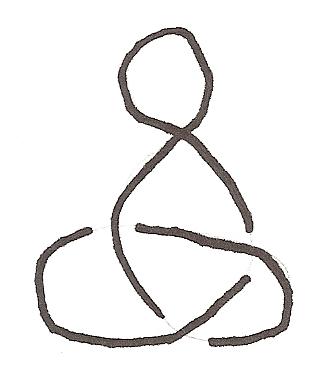
Figure 13.1: One move remains, but King Lear has already won.

On the other hand,

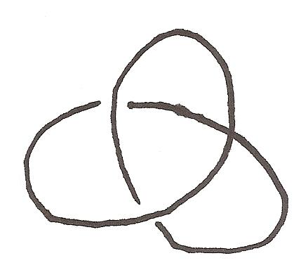
Figure 13.2: The next move decides and ends the game.

is $\langle 0,1|0,1\rangle\approx\langle 1|0\rangle$, because the remaining crossing decides whether the resulting knot will be a knotted trefoil or an unknot.

The natural way to add TKONTK positions is the $\oplus_{2}=\vee$ operation of Section 12.5. For example, when we add Figures 13.1 and 13.2 ,

we get a position with value $\{1|0\}\vee 1*\approx\{1|1\}+*\approx 1.$ So the resulting position is equivalent to, say

13.1 Phony Reidemeister Moves

Definition 13.1.1.

A pseudodiagram $S$ is obtained by a phony Reidemeister I move from a pseudodiagram $T$ if $S$ is obtained from $T$ by removing a loop with an unresolved crossing from $T$, as in Figure 13.3. We denote this $T\stackrel{{\scriptstyle 1}}{{\rightarrow}}S$.

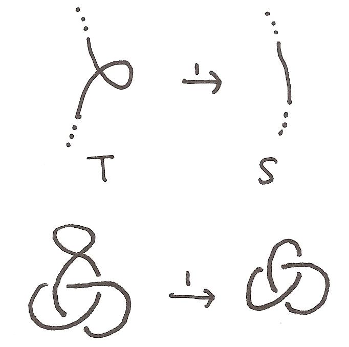
Figure 13.3: Phony Reidemeister I move

Definition 13.1.2.

A pseudodiagram $S$ is obtained by a phony Reidemeister II move from a pseudodiagram $T$ if $S$ is obtained from $T$ by uncrossing two overlapped strings, as in Figure 13.4, where the two crossings eliminated are unresolved. We denote this $T\stackrel{{\scriptstyle 2}}{{\rightarrow}}S$.

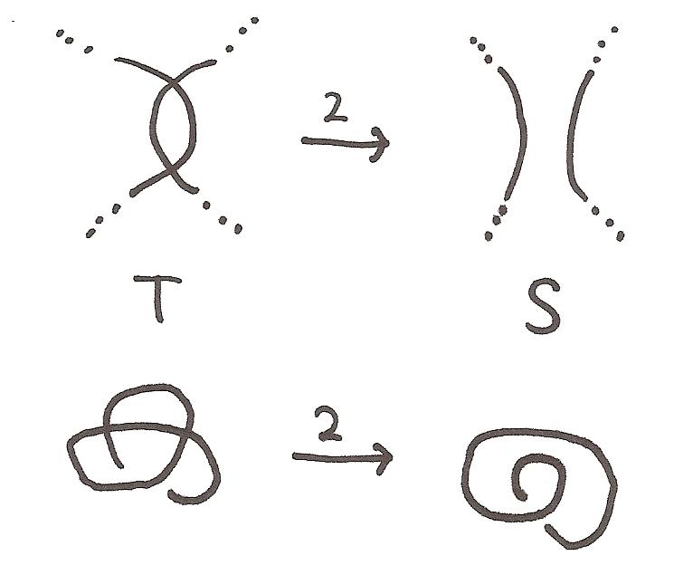
Figure 13.4: Phony Reidemeister II move

Note that we only use these operations in one direction: $T\stackrel{{\scriptstyle i}}{{\rightarrow}}S$ doesn’t imply $S\stackrel{{\scriptstyle i}}{{\rightarrow}}T$. We also use the notation $T\stackrel{{\scriptstyle i}}{{\Rightarrow}}S$ to indicate that $S$ is obtained from $T$ by a sequence of zero or more type $i$ moves, and $T\stackrel{{\scriptstyle*}}{{\Rightarrow}}S$ to indicate that $S$ is obtained by zero or more moves of either type.

If $T$ is a knot pseudodiagram, we let $\operatorname{val}(T)$ be the value of $T$ as a game of TKONTK, and we abuse notation and write $u^{+}(T)$ and $u^{-}(T)$ for $u^{+}(\operatorname{val}(T))$ and $u^{-}(\operatorname{val}(T))$.

The importance of the phony Reidemeister moves is the following:

Theorem 13.1.3.

If $T\stackrel{{\scriptstyle 1}}{{\rightarrow}}S$ then $\operatorname{val}(T)=\operatorname{val}(S)+*$, so $u^{+}(T)=u^{+}(S)$ and $u^{-}(T)=u^{-}(S)$.

If $T\stackrel{{\scriptstyle 2}}{{\rightarrow}}S$, then $\operatorname{val}(T)\gtrsim_{+}\operatorname{val}(S)$ and $\operatorname{val}(T)\lesssim_{-}\operatorname{val}(S)$. So $u^{+}(T)\geq u^{+}(S)$ and $u^{-}(T)\leq u^{-}(S)$.

Proof.

If $S$ is obtained from $T$ by a phony Reidemeister I move, then $T$ is obtained from $S$ by adding an extra loop (with an unresolved crossing). In other words $T$ is $S\#K$ where $K$ is the following pseudodiagram:

As noted above, $\operatorname{val}(K)=*$, so

$$\operatorname{val}(T)=\operatorname{val}(S)\oplus_{2}*=\operatorname{val}(S)\oplus_{2}(0+*)=(\operatorname{val}(S)+*)\oplus_{2}=\operatorname{val}(S)+*,$$

using Lemma 10.1.6 and the fact that $0$ is the identity element for $\oplus_{2}$.

For the second claim, we need to show that undoing a phony Reidemeister II move does not hurt whichever player moves last, even if the pseudodiagram is being added to an arbitrary integer-valued game. To see this, suppose that $T\stackrel{{\scriptstyle 2}}{{\rightarrow}}S$ and that Alice have a strategy guaranteeing a certain score in $\operatorname{val}(S)+G$ for some $G\in\mathcal{W}_{\mathbb{Z}}$, when Alice is the player who will make the last move. Then Alice can use this same strategy in $\operatorname{val}(T)+G$, except that she applies a pairing strategy to manage the two new crossings. If her opponent moves in one, then she moves in the other, in a way that produces one of the following configurations:

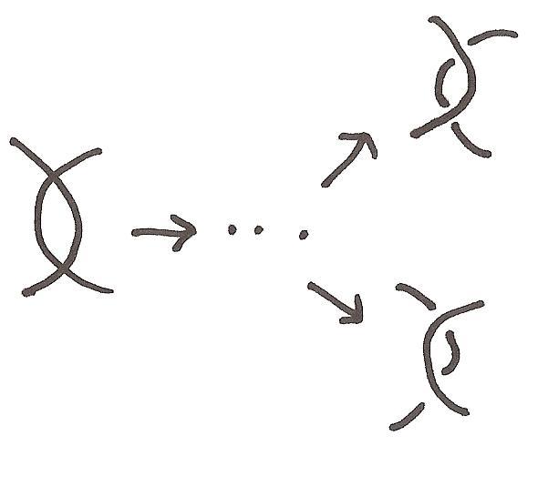
Figure 13.5: After the first move, it is always possible to reply with a move to one of the configurations on the right.

Otherwise, she does not move in either of the two new crossings, and pretends that she is in fact playing $\operatorname{val}(S)+G$. Since she is the player who will make the last move in the game, she is never forced to move in one of the two crossings before her opponent does, so this pairing strategy always works. And if the two crossings end up in one of the configurations on the right side of Figure 13.5, then they can be undone by a standard Reidemeister II move, yielding a position identical to the one that Alice pretends she has reached, in $\operatorname{val}(S)+G$. Since Alice had a certain guaranteed score in $\operatorname{val}(S)+G$, she can ensure the same score in $\operatorname{val}(T)+G$. This works whether Alice is Left or Right, so we are done. ∎

13.2 Rational Pseudodiagrams and Shadows

We use $[]$ to denote the rational tangle

and $[a_{1},\ldots,a_{n}]$ to denote the rational tangle obtained from $[a_{1},\ldots,a_{n-1}]$ by reflection over a 45 degree axis and adding $a_{n}$ twists to the right. We also generalize this notation, letting $[a_{1}(b_{1}),\ldots,a_{n}(b_{n})]$ denote a tangle-like pseudodiagram in which there are $a_{1}$ legitimate crossings and $b_{1}$ unresolved crossings at each step. See Figure 13.6 for examples.

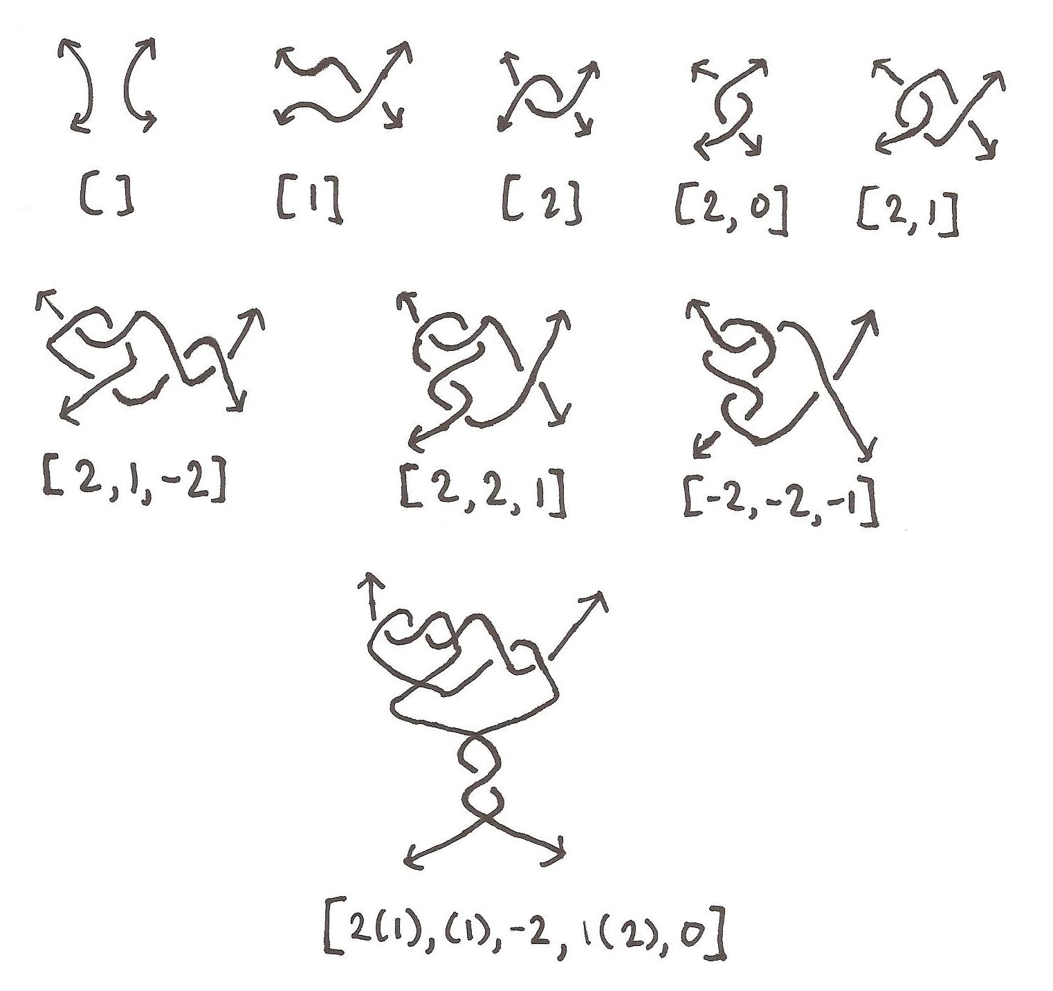
Figure 13.6: Examples of our notation.

So the $a_{i}\in\mathbb{Z}$ and the $b_{i}\in\mathbb{N}$, where $\mathbb{N}$ are the nonnegative integers. If $a_{i}=0$, we write $(b_{i})$ instead of $a_{i}(b_{i})$, and similarly if $b_{i}=0$, we write $a_{i}$ instead of $a_{i}(b_{i})$. A shadow is a pseudodiagram in which all crossings are unresolved, so a rational shadow tangle would be of the form $[(b_{1}),\ldots,(b_{n})]$.

We abuse notation, and use the same $[a_{1}(b_{1}),\ldots,a_{n}(b_{n})]$ notation for the pseudodiagram obtained by connecting the top two strands of the tangle and the bottom two strands:

Note that this can sometimes yield a link, rather than a knot:

We list some fundamental facts about rational tangles:

Theorem 13.2.1.

If $[a_{1},\ldots,a_{m}]$ and $[b_{1},\ldots,b_{n}]$ are rational tangles, then they are equivalent if and only if

$$a_{m}+\frac{1}{a_{m-1}+\frac{1}{\ddots+\frac{1}{a_{1}}}}=b_{n}+\frac{1}{b_{n-1}+\frac{1}{\ddots+\frac{1}{b_{1}}}}.$$

The knot or link $[a_{1},\ldots,a_{m}]$ is a knot (as opposed to a link) if and only if

$$a_{m}+\frac{1}{a_{m-1}+\frac{1}{\ddots+\frac{1}{a_{1}}}}=\frac{p}{q},$$

where $p,q\in\mathbb{Z}$ and $p$ is odd. Finally, $[a_{1},\ldots,a_{m}]$ is the unknot if and only if $q/p$ is an integer.

Note that $[a_{1}(b_{1}),\ldots,a_{n}(b_{n})]$ is a knot pseudodiagram (as opposed to a link pseudodiagram) if and only if $[a_{1}+b_{1},\ldots,a_{n}+b_{n}]$ is a knot (as opposed to a link), since the number of components in the diagram does not depend on how crossings are resolved.

The proofs of the following lemmas are left as an exercise to the reader. They are easily seen by drawing pictures, but difficult to prove rigorously without many irrelevant details.

Lemma 13.2.2.

The following pairs of rational shadows are topologically equivalent (i.e., equivalent up to planar isotopy):

$$\left[(1),(a_{1}),\ldots,(a_{n})\right]=\left[(a_{1}+1),(a_{2})\ldots,(a_{n})\right]$$ (13.1)

$$\left[(a_{1}),\ldots,(a_{n}),(1)\right]=\left[(a_{1}),\ldots,(a_{n-1}),(a_{n}+1)\right]$$ (13.2)

$$\left[(0),(0),(a_{1}),\ldots,(a_{n})\right]=\left[(a_{1}),\ldots,(a_{n})\right]$$ (13.3)

$$\left[(a_{1}),\ldots,(a_{i}),(0),(a_{i+1}),\ldots,(a_{n})\right]=\left[(a_{1}),\ldots,(a_{i}+a_{i+1}),\ldots,(a_{n})\right]$$ (13.4)

$$\left[(a_{1}),\ldots,(a_{n}),0,0\right]=\left[(a_{1}),\ldots,(a_{n})\right]$$ (13.5)

$$\left[(a_{1}),(a_{2}),\ldots,(a_{n})\right]=\left[(a_{n}),\ldots,(a_{2}),(a_{1})\right]$$ (13.6)

Only (13.6) is non-obvious. The equivalence here follows by turning everything inside out, as in Figure 13.7.

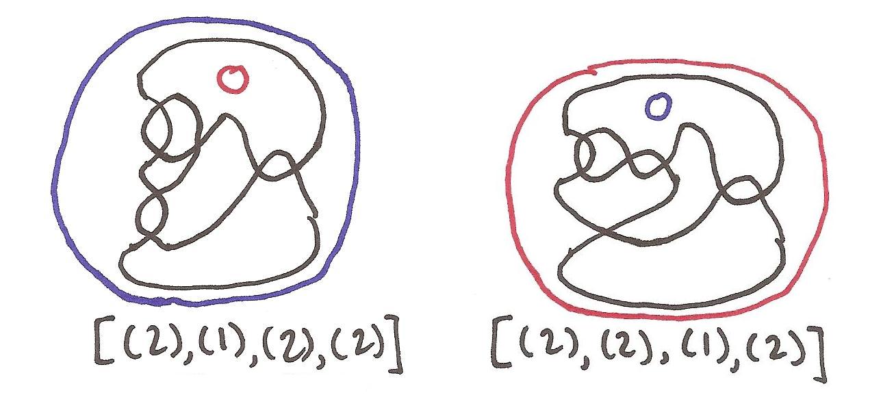
Figure 13.7: These two knot shadows are essentially equivalent. One is obtained from the the other by turning the diagram inside out, exchanging the red circle on the inside and the blue circle on the outside.

This works because the diagram can be thought of as living on the sphere, mainly because the following operation has no effect on a knot:

Figure 13.8: Moving a loop from one side of the knot to the other has no effect on the knot. So we might as well think of knot diagrams as living on the sphere.

Similarly, we also have

Lemma 13.2.3.

$$\left[(0),(a_{1}+1),(a_{2}),\ldots,(a_{n})\right]\stackrel{{\scriptstyle 1}}{{\rightarrow}}\left[(0),(a_{1}),(a_{2}),\ldots,(a_{n})\right]$$ (13.7)

$$\left[(a_{1}),\ldots,(a_{n-1}),(a_{n}+1),0\right]\stackrel{{\scriptstyle 1}}{{\rightarrow}}\left[(a_{1}),\ldots,(a_{n-1}),(a_{n}),0\right]$$ (13.8)

$$\left[\ldots,(a_{i}+2),\ldots\right]\stackrel{{\scriptstyle 2}}{{\rightarrow}}\left[\ldots,(a_{i}),\ldots\right]$$ (13.9)

Note that $[]$ is the unknot.

Lemma 13.2.4.

If $T$ is a rational shadow, that resolves to be a knot (not a link), then $T\stackrel{{\scriptstyle*}}{{\Rightarrow}}[]$.

Proof.

Let $T=\left[(a_{1}),\ldots,(a_{n})\right]$ be a minimal counterexample. Then $T$ cannot be reduced by any of the rules specified above. Since any $a_{i}\geq 2$ can be reduced by (13.9), all $a_{i}<2$. If $n=0$, then $T=\left[\right]$ which turns out to be the unknot. If $a_{0}=0$ and $n>1$, then either $a_{1}$ can be decreased by $1$ using (13.7), or $a_{0}$ and $a_{1}$ can be stripped off via (13.3). On the other hand, if $a_{0}=0$ and $n=1$, then $T=\left[(0)\right]$, which is easily seen to be a link (not a knot). So $a_{0}=1$. If $n>1$, then $T$ reduces to $\left[(a_{2}+1),\ldots,(a_{n})\right]$ by (13.1). So $n=1$, and $T$ is $\left[(1)\right]$ which clearly reduces to the unknot via a phony Reidemeister I move:

∎

Because of this, we see that every rational shadow has downside $0$ or $*$, viewed as a TKONTK position:

Theorem 13.2.5.

Let $T$ be a rational knot shadow (not a link). Then $\operatorname{val}(T)\approx_{-}0$ or $\operatorname{val}(T)\approx_{-}*$.

Proof.

By the lemma, $T\stackrel{{\scriptstyle*}}{{\Rightarrow}}[]$. But then by Theorem 13.1.3, $u^{-}(T)\leq u^{-}([])=0$, since $\operatorname{val}([])=0$ and $u^{-}(0)=0$. But the only possible values for $u^{-}(T)$ are $0,\frac{1}{4},\frac{3}{8},\ldots$, so $u^{-}(T)\leq 0$ implies that $u^{-}(T)=0$. Then $\operatorname{val}(T)$ is equivalent to either $0$ or $*$. ∎

Now $\lceil 0\rceil=0$ and $\lfloor 0+\frac{1}{2}\rfloor=0$, so by Corollary 12.3.8, we see that if $T$ is a rational shadow with an even number of crossings, then $\operatorname{L}(\operatorname{val}(T))=0$, and if $T$ has an odd number of crossings, then $\operatorname{R}(\operatorname{val}(T))=0$. So in particular, there are no rational shadows for which King Lear can win as both first and second player. And since games with $u^{-}(G)=0$ are closed under $\oplus_{2}$, the same is true for any position which is a connected sum of rational knot shadows.

Rational pseudodiagrams, on the other hand, can be guaranteed wins for King Lear. For example, in $[0,(1),3]$, King Lear can already declare victory:

13.3 Odd-Even Shadows

Definition 13.3.1.

An odd-even shadow is a shadow of the form

$$\left[(a_{1}),(a_{2}),\ldots,(a_{n})\right],$$

where all $a_{i}\geq 1$, exactly one of $a_{1}$ and $a_{n}$ is odd, and all other $a_{i}$ are even.

Note that these all have an odd number of crossings (so they yield odd-tempered games). It is straightforward to verify from (13.1-13.9) that every odd-even shadow reduces by phony Reidemeister moves to the unknot. In particular, by repeated applications of (13.9), we reduce to either $[(0),\ldots,(0),(1)]$ or $[(1),(0),\ldots,(0)]$. Then by applying (13.3) or (13.5), we reach one of the following:

$$[(1)],[(0),(1)],[(1),(0)].$$

Then all of these are equivalent to $[(1)]$ by (13.1) or (13.2). So since every odd-even shadow reduces to the unknot, ever odd-even shadow is an actual knot shadow, not a link shadow. Thus any odd-even shadow can be used as a game of TKONTK.

Theorem 13.3.2.

If $T$ is an odd-even shadow, then $u^{+}(T)=0$.

Proof.

Suppose that $\operatorname{L}(\operatorname{val}(T)\oplus_{2}\langle 0|1\rangle\oplus_{2}*)=0$. Then by Corollary 12.3.8,

$$\left\lceil(u^{+}(T)\cup u^{+}(\langle 0|1\rangle)\cup u^{+}(*))-\frac{1}{2}\right\rceil=0,$$

since $\operatorname{val}(T)\oplus_{2}\langle 0|1\rangle\oplus_{2}*$ is odd-tempered. But $u^{+}(*)=0$, $u^{+}(\langle 0|1\rangle)=\frac{1}{2}$, and $\frac{1}{2}\cup 0=\frac{1}{2}$. And $\lceil x\rceil\leq 0$ if and only if $x\leq 0$. So

$$u^{+}(T)\cup\frac{1}{2}\leq\frac{1}{2}.$$

But if $u^{+}(T)\neq 0$, then $u^{+}(T)\geq\frac{1}{4}$, so that $u^{+}(T)\cup\frac{1}{2}\geq\frac{1}{4}\cup\frac{1}{2}=\frac{3}{4}\not\leq\frac{1}{2}$, a contradiction. So it suffices to show that

$$\operatorname{L}(\operatorname{val}(T)\oplus_{2}\langle 0|1\rangle\oplus_{2}*)=0,$$

i.e., that Ursula has a winning strategy as the second player in

$$\operatorname{val}(T)\oplus_{2}G$$ (13.10)

where $G=\langle 0|1\rangle\oplus_{2}*=\langle 0|1\rangle+*$.

Let $T=[(a_{1}),\ldots,(a_{n})]$. Suppose first that $a_{1}$ is odd and the other $a_{i}$ are even. Then Ursula’s strategy in (13.10) is to always move to a position of one of the following forms:

(A)

$\operatorname{val}([(b_{1}),\ldots,(b_{m})])\oplus_{2}G^{\prime}$, where $b_{1}$ is odd and the other $b_{i}$ are even, and $G^{\prime}$ is $G$ or $0$.

(B)

$\operatorname{val}([1(b_{1}),\ldots,(b_{m})])\oplus_{2}G^{\prime}$, where the $b_{i}$ are all even and $G^{\prime}$ is an odd-tempered subposition of $G$.

Note that the initial position is of the first form, with $b_{i}=a_{i}$ and $G^{\prime}=G$. To show that this is an actual strategy, we need to show that Ursula can always move to a position of one of the two forms.

• In a position of type (A), if Lear moves in one of the $b_{i}$, from $(b_{i})$ to $\pm 1(b_{i}-1)$, then Ursula can reply with a move to $(b_{i}-2)$, as in Figure 13.9, unless $b_{i}=1$.

  

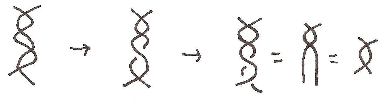
  Figure 13.9: Ursula responds to a twisting move by King Lear with a cancelling twist in the opposite direction.

  But if $b_{i}=1$, then King Lear has just moved to

  $$\operatorname{val}([\pm 1,(b_{2}),\ldots,(b_{n})])\oplus_{2}G^{\prime}=\operatorname{val}([\pm 1(b_{2}),\ldots,(b_{n})])\oplus_{2}G^{\prime},$$

  using the fact that $[\pm 1,(b_{2}),\ldots,(b_{n})]=[\pm 1(b_{2}),(b_{3}),\ldots,(b_{n})]$ (obvious from a picture). So now Ursula can reply using $b_{2}$ instead of $b_{1}$, and move back to a position of type $A$, unless King Lear has just moved to

  $$\operatorname{val}([\pm 1])\oplus_{2}G^{\prime}.$$

  But $[\pm 1]$ are unknots, so $\operatorname{val}([\pm 1])=0$, and $G^{\prime}$ is $0$ or $G$, both of which are first player wins for Ursula, so King Lear has made a losing move.

• In a position of type (A), if Lear moves in $G^{\prime}=G$ to $0+*$, then Ursula replies by moving from $0+*$ to $0+0$, getting back to a position of type (A).

• In a position of type (A), if Lear moves in $G^{\prime}=G$ to $\langle 0|1\rangle+0$, then Ursula moves $(b_{1})\to 1(b_{1}-1)$, creating a position of type (B).

• In a position of type (B), if Lear moves in $G^{\prime}$ to $0$ (this is the only left option of either possibility for $G^{\prime}$), then Ursula replies with a move from $1(b_{1})$ to $0(b_{1}-1)$, where $0=1-1$. This works as long as $b_{1}\neq 0$. But if $b_{1}=0$, then we could have rewritten $[1(b_{1}),(b_{2}),\ldots]$ as $[1(b_{2}),(b_{3}),\ldots]$ as before. If $b_{2}=0$ too, then we can keep on sliding over, until eventually Ursula finds a move, or it turns out that King Lear moved to a position of the form

  $$[1]\oplus_{2}0$$

  which is $0$, a win for Ursula.

• In a position of type (B), if Lear moves in any $b_{i}$, then Ursula makes the cancelling move

  $$(b_{i})\to\pm 1(b_{i}-1)\to 0(b_{i}-2),$$

  this is always possible because if $b_{i}\geq 1$, then $b_{i}\geq 2$.

From the discussion above, Ursula can keep following this strategy until Lear makes a losing move. So this is a winning strategy for Ursula and we are done.

The other case, in which $a_{n}$ is odd and the other $a_{i}$ are even, is handled completely analogously. ∎

13.4 The other games

Lemma 13.4.1.

The following rational shadows have $u^{+}(T)=1$:

$$\left[(3),(1),(3)\right],\left[(2),(1),(2),(2)\right],\left[(2),(2),(1),(2)\right],\left[(2),(1),(1),(2)\right],$$

$$\left[(2),(2),(1),(2),(2)\right],\left[(2),(2)\right]$$

Proof.

To show that $u^{+}(T)=1$, it suffices by Corollary 12.3.8 to show that $G$ is a win for King Lear when Ursula moves first, where $G$ is $\operatorname{val}(T)$ if $T$ has an even number of crossings, and $G$ is $\operatorname{val}(T)+*$ otherwise. For $\operatorname{R}(G)=1$ iff $\lfloor u^{+}(G)\rfloor=1$, which happens if and only if $1\leq u^{+}(G)=u^{+}(T)$.

Unfortunately, the only way I know to prove this criterion for all the knots listed above is by computer, making heavy use of Theorem 13.2.1. ∎

These are shown in Figure  13.10.

Figure 13.10: The shadows of Lemma 13.4.1.

Lemma 13.4.2.

If $T=\left[(a_{1}),\ldots,(a_{n})\right]$ is a rational shadow corresponding to a knot (not a link) with at least one crossing, then either $T\stackrel{{\scriptstyle 1}}{{\Rightarrow}}O$ for some odd-even shadow $O$, or $T\stackrel{{\scriptstyle*}}{{\Rightarrow}}A$, where $A$ is equivalent to one of the six shadows in Lemma 13.4.1.

Proof.

Without loss of generality, $T$ is irreducible as far as phony Reidemeister I moves go. Then we can make the assumption that all $a_{i}>0$. If all of the $a_{i}$ are even, then by applying (13.9) and (13.3-13.5), we can reduce $T$ down to either $\left[(2),(2)\right]$ or $\left[(2)\right]$. But the second of these is easily seen to be a link, so $T\stackrel{{\scriptstyle*}}{{\Rightarrow}}\left[(2),(2)\right]$. Otherwise, at least one of the $a_{i}$ is odd. If the only odd $a_{i}$ are $i=1$ and/or $i=n$, then either $T$ is an odd-even shadow, or $a_{1}$ and $a_{n}$ are both odd. But if both $a_{1}$ and $a_{n}$ are odd, then by applying (13.9) and (13.4), we can reduce to one of the cases $\left[(1),(0),(1)\right]$ or $\left[(1),(1)\right]$. By (13.4) or (13.1), both of these are equivalent to $\left[(2)\right]$, which is not a knot.

This leaves the case where at least one $a_{i}$ is odd, $1<i<n$. Let $T$ be (a) not reducible by phony Reidemeister I moves or by (13.1-13.2), and (b) as reduced as possible by phony Reidemeister II moves, without breaking the property of having one of the $a_{i}$ be odd, for $1<i<n$. If $a_{j}>2$ for any $1<j<n$, then we can reduce $a_{j}$ by two, via (13.9). So for every $1<j<n$, $a_{j}\leq 2$. Similarly, $a_{1}$ and $a_{n}$ must be either $2$ or $3$. (They cannot be $1$ or else $T$ would be reducible by (13.1) or (13.2).)

Choose $i$ for which $a_{i}$ is odd. If $a_{1}=3$ and $i>2$, then we can reduce $a_{1}$ by two (13.9) and combine it (13.1) into $a_{2}$ to yield a smaller $T$. So if $a_{1}=3$, then $a_{2}=1$ and $a_{j}\neq 1$ for $j>2$ (or else we could have chosen a different $i$ and reduced). Similarly, if $a_{n}=3$, then $a_{n-1}=1$ and $a_{j}\neq 1$ for $j<n-1$. Thus, if a sequence begins with $(3)$, the next number must be $(1)$, and the $(1)$ must be unique. For example, the sequence $\left[(3),(1),(1),(3)\right]$ can be reduced to $\left[(1),(1),(1),(3)\right]$ and thence to $\left[(2),(1),(3)\right]$.

On the other hand, suppose $a_{1}=2$. If $i>4$ then we can reduce $T$ farther by decreasing $a_{1}$ by (13.9), and then decreasing $a_{2}$ one by one via (13.7) until both $a_{1}$ and $a_{2}$ are zero. Then both can be removed by (13.3), yielding a smaller $T$. A further application of (13.1) may be necessary to remove an initial 1. Moreover, if (13.1) is unnecessary, because $a_{3}>1$, then this also works if $i=4$.

Therefore, what precedes any $a_{i}=1$ must be one of the following:

• $(3)$

• $(2)$

• $(2)(2)$

• $(2)(1)$

• $(2)(2)(1)$

• $(2)(1)(1)$

and only the first three of these can precede the first $(1)$. The same sequences reversed must follow any $(1)$ in sequence. Then the only combinations which can occur are:

• $\left[(3),(1),(3)\right]$

• $\left[(3),(1),(2)\right]$ and its reverse

• $\left[(3),(1),(2),(2)\right]$ and its reverse

• Not $\left[(3),(1),(1),(2)\right]$ because more than just $(3)$ precedes the second $(1)$.

• $\left[(2),(1),(2)\right]$

• $\left[(2),(1),(2),(2)\right]$ and its reverse

• $\left[(2),(1),(1),(2)\right]$

• $\left[(2),(1),(1),(2),(2)\right]$ and its reverse

• $\left[(2),(1),(1),(1),(2)\right]$

• $\left[(2),(2),(1),(2),(2)\right]$

• $\left[(2),(2),(1),(1),(2),(2)\right]$

• Not $\left[(2),(2),(1),(1),(1),(2)\right]$ because too much precedes the last $(1)$.

So either $T$ is one of the combinations in Lemma 13.4.1 or one of the following happens:

• $\left[(3),(1),(2)\right]$ reduces by (13.9) to $\left[(1),(1),(2)\right]=\left[(2),(2)\right]$. So does its reverse.

• $\left[(3),(1),(2),(2)\right]$ reduces by two phony Reidemeister II moves to

  $$\left[(3),(1),(0),(0)\right]=\left[(3),(1)\right]=\left[(4)\right]$$

  which is a link, not a knot. Nor is its reverse.

• $\left[(2),(1),(2)\right]$ reduces by a phony Reidemeister II move to $\left[(0),(1),(2)\right]$, which in turn reduces by a phony Reidemeister I move to $\left[(0),(0),(2)\right]=\left[(2)\right]$ which is a link, not a knot. So this case can’t occur.

• $\left[(2),(1),(1),(2),(2)\right]$ reduces by phony Reidemeister moves to

  $$\left[(2),(1),(1),(0),(2)\right]=\left[(2),(1),(3)\right]$$

  so it isn’t actually minimal.

• $\left[(2),(1),(1),(1),(2)\right]$ likewise reduces by a phony Reidemeister II move and a I move to

  $$\left[(0),(0),(1),(1),(2)\right]=\left[(1),(1),(2)\right]=\left[(2),(2)\right]$$

• $\left[(2),(2),(1),(1),(2),(2)\right]$ reduces by a phony Reidemeister II move to

  $$\left[(2),(0),(1),(1),(2),(2)\right]=\left[(3),(1),(2),(2)\right],$$

  so it isn’t actually minimal.

In summary then, every $T$ that does not reduce by phony Reidemeister I moves to an odd-even shadow reduces down to a finite set of minimal cases. Each of these minimal cases is either reducible to one of the six shadows in Lemma 13.4.1, or is not actually a knot. ∎

13.5 Sums of Rational Knot Shadows

Putting everything together we have

Theorem 13.5.1.

Let $T$ be a rational knot shadow, and let $T^{\prime}=\left[a_{1},a_{2},\ldots,a_{n}\right]$ be the smallest $T^{\prime}$ such that $T\to_{1}^{*}T^{\prime}$. Then if $T^{\prime}$ is an odd-even shadow, $T$, $u^{+}(T)=u^{-}(T)=0$, and otherwise, $u^{+}(T)=1$, $u^{-}(T)=0$.

Proof.

We know that $\operatorname{val}(T^{\prime})$ and $\operatorname{val}(T)$ differ by $0$ or $*$, so $u^{+}(T)=u^{+}(T^{\prime})$ and $u^{-}(T)=u^{-}(T^{\prime})$. We already know that if $T^{\prime}$ is an odd-even shadow, then $u^{-}(T^{\prime})=0$. Otherwise, by Lemma 13.4.2, $T^{\prime}$ must reduce by phony Reidemeister I and II moves to a rational shadow $T^{\prime\prime}$ that is one of the six shadows in Lemma 13.4.1. By Lemma 13.4.1, $u^{+}(T^{\prime\prime})=1$. Then by Theorem 13.1.3, $u^{+}(T)\geq u^{+}(T^{\prime})\geq u^{+}(T^{\prime\prime})$. But $u^{+}(T^{\prime\prime})$ is already the maximum value $1$, so $u^{+}(T)=1$ too. On the other hand, we know that $u^{-}(T)=0$ by Theorem 13.2.5, regardless of what $T$ is. ∎

Definition 13.5.2.

A rational knot shadow reduces to an odd-even shadow if it reduces to an odd-even shadow via phony Reidemeister I moves.

The previous theorem can be restated to say that a rational knot shadow has $u^{+}=0$ if it reduces to an odd-even shadow, and $u^{+}=1$ otherwise.

Theorem 13.5.3.

If $T_{1},T_{2},\ldots T_{n}$ are rational knot shadows, and $T=T_{1}+T_{2}+\ldots+T_{n}$ is their connected sum, then $T$ is a win for Ursula if all of the $T_{i}$ reduce to odd-even shadows. Otherwise, if $T$ has an odd number of crossings, then $T$ is a win for whichever player goes first, and if $T$ has an even number of crossings, then $T$ is a win for whichever player goes second.

Proof.

Note that $0\cup 0=0$ and $1\cup 0=1\cup 1=1$. So by Theorem 13.5.1, if every $T_{i}$ reduces to an odd-even shadow, then $u^{\pm}(T_{1}+\cdots+T_{n})=0$. So then $\operatorname{val}(T_{1}+\cdots+T_{n})\approx 0$, and so $T_{1}+\cdots+T_{n}$ is a win for Right (Ursula) no matter who goes first.

Otherwise, it follows by Theorem 13.5.1 that $u^{-}(T_{1}+\cdots+T_{n})=0$ and $u^{+}(T_{1}+\cdots+T_{n})=1$. So by Corollary 12.3.8, if $\operatorname{val}(T_{1}+\cdots+T_{n})$ is even-tempered, then

$$\operatorname{L}(\operatorname{val}(T_{1}+\cdots+T_{n}))=\lceil 0\rceil=0$$

so that Ursula wins if King Lear goes first, and

$$\operatorname{R}(\operatorname{val}(T_{1}+\cdots+T_{n}))=\lfloor 1\rfloor=1$$

so that King Lear wins if Ursula goes first.

On the other hand, if $\operatorname{val}(T_{1}+\cdots+T_{n})$ is odd-tempered, then

$$\operatorname{L}(\operatorname{val}(T_{1}+\cdots+T_{n}))=\lceil 1-\frac{1}{2}\rceil=1$$

so that King Lear wins when he goes first, and similarly

$$\operatorname{R}(\operatorname{val}(T_{1}+\cdots+T_{n}))=\lfloor 0-\frac{1}{2}\rfloor=0$$

so that Ursula wins when she goes first. ∎

13.6 Computer Experiments and Additional Thoughts

So far, we have determined the value of rational shadows, that is, rational pseudodiagrams in which no crossings are resolved. Although we have “solved” the instances of To Knot or Not to Knot that correspond to rational knots, we have not strongly solved them, by finding winning strategies in all their subpositions. This would amount to determining the values of all rational pseudodiagrams.

Since rational pseudodiagrams resolve to rational knots, a computer can check whether the outcome of a game is knotted or not. I wrote a program to determine the values of small rational pseudodiagrams. Interestingly, the only values of $u^{+}$ and $u^{-}$ which appeared were $0$, $1$, and $\frac{1}{2}*$. This also appeared when I analyzed the positions of the following shadow:

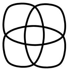
Figure 13.11: The simplest shadow which does not completely reduce via phony Reidemeister I and II moves.

which is the simplest shadow which does not reduce via phony Reidemeister I and II moves to the unknot. So Theorem 13.2.5 does not apply, and in fact, by a computer, I verified that this knot does not have $u^{-}=0$.

Since Figure 13.11 is not a rational shadow or sum of rational shadows, I used another invariant called the knot determinant to check whether the final resolution was an unknot.

Definition 13.6.1.

Let $K$ be a knot diagram with $n$ crossings and $n$ strands. Create a matrix $M$ such that $M_{ij}$ is -1 if the $i$th strand terminates at the $j$th crossing, 2 if the $i$th strand passes over the $j$th crossing, and 0 otherwise. The knot determinant is defined as $|\det(M^{\prime})|$, where $M^{\prime}$ is any $(n-1)\times(n-1)$ submatrix of $M$.

It turns out that the knot determinant is well defined, and is even a knot invariant. In fact, if $\Delta(z)$ is the Alexander polynomial, then the knot determinant is just $|\Delta(-1)|$. The knot determinant of the unknot equals 1.

Lemma 13.6.2.

If the knot shadow in Figure 13.11 is resolved into a knot $K$, then $K$ is the unknot iff the knot determinant of $K$ equals 1.

Proof.

We can use a computer to check whether a resolution of the diagram has knot determinant 1. There are only 256 resolutions, so it is straightforward to iterate over all resolutions. Up to symmetry, it turns out that the only resolutions with knot determinant 1 are those shown in Figure 13.12. It is straightforward to check that all of these are the unknot. Conversely, any knot whose determinant is not 1 cannot be the unknot, since the knot determinant is a knot invariant. ∎

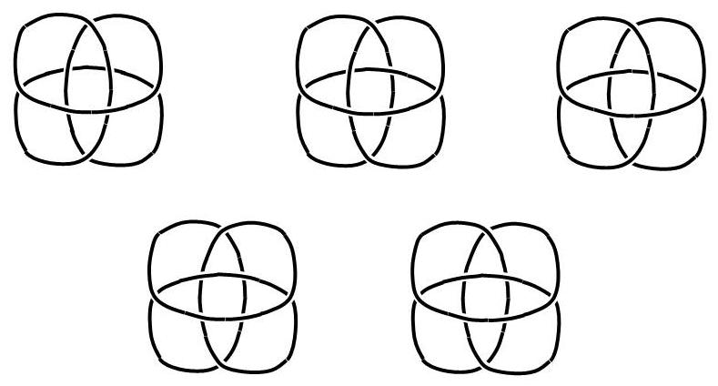
Figure 13.12: Up to symmetry, these are the only ways to resolve Figure 13.11 and have the knot determinant equal 1. They are all clearly the unknot.

Because of this, we can use a computer to determine the value of the game played on the diagram in Figure 13.11. The value turned out to be $u^{+}=1$. Then by Corollary 12.3.8, this game is a win for King Lear, no matter who goes first. This answers a question posed in A Midsummer Knot’s Dream.

The program used to analyze the shadow of Figure 13.11 also determined the values that occur in subpositions of this game. Again, only the values $0$, $1$, and $\frac{1}{2}*$ were seen for $u^{\pm}$ values.

This led me to conjecture that these were the only possible values for any knot pseudodiagrams. However, it seems very unlikely that this could be due to some special property of knots. In fact, it seems like it might be true of a larger class of games, in which Left and Right take turns setting the arguments of a fixed function $f:\{0,1\}^{n}\to\{0,1\}$, and then the value of $f$ determines who wins.

I tried for a long time to prove that for such games, the only possible $u^{\pm}$ values were $0$, $1$, and $\frac{1}{2}*$. This was unlikely, for the following reason:

Theorem 13.6.3.

If $G$ is an odd-tempered Boolean game, and $u^{\pm}(G)\in\{0,1,\frac{1}{2}*\}$, then $G$ is not a second-player win.

Proof.

If $G$ is a first-player win, then $\operatorname{L}(G)=0$ and $\operatorname{R}(G)=1$. By Corollary 12.3.8, this means that

$$0=\lceil u^{+}(G)-\frac{1}{2}\rceil,$$

so that $u^{+}(G)\leq\frac{1}{2}$. Similarly,

$$1=\lfloor u^{-}(G)+\frac{1}{2}\rfloor,$$

so that $u^{-}(G)\geq\frac{1}{2}$. Then we have

$$\frac{1}{2}\leq u^{-}(G)\leq u^{+}(G)\leq\frac{1}{2},$$

so that $u^{-}(G)=u^{+}(G)=\frac{1}{2}$, a contradiction. ∎

Projective Hex is a positional game like Hex, in which the two players take turns placing pieces of their own colors on a board until somebody creates a path having a certain property. In Hex, the path needs to connect your two sides of the board, but in projective Hex, played on a projective plane, the path needs to wrap around the world an odd number of times:

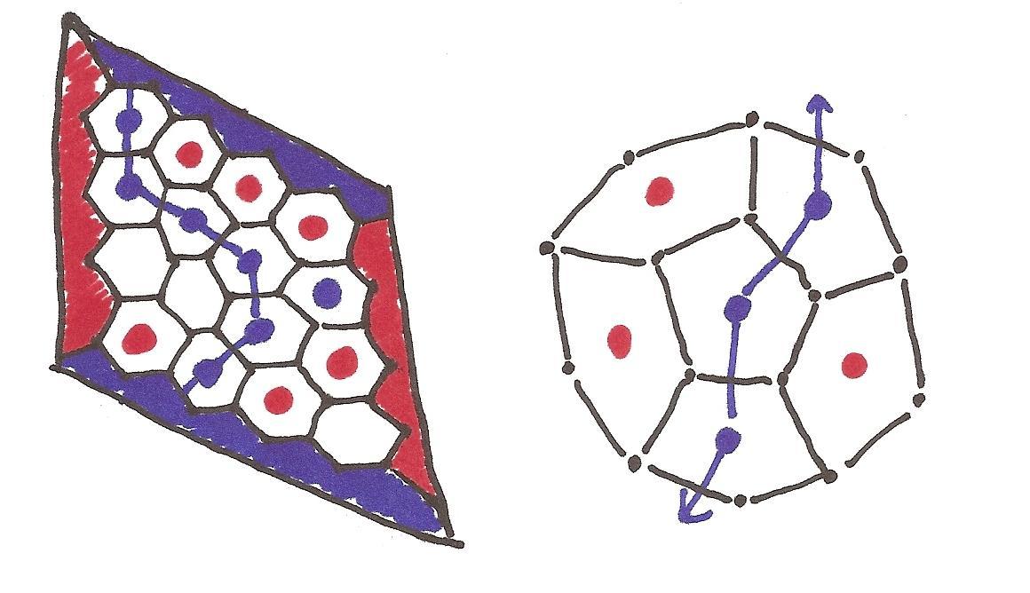
Figure 13.13: Hex (left) and Projective Hex (right, here played on the faces of a dodecahedron). In both games, Blue has won. In the Hex game, she connected her two sides, and in the Projective Hex game, she created a path which wrapped around the world an odd number of times.

By a standard strategy-stealing argument, Hex and Projective Hex are necessarily wins for the first player. When Projective Hex is played on the faces of a dodecahedron (or rather on the pairs of opposite faces) it has the property that every opening move is a winning move, by symmetry.

Now modify dodecahedral projective hex by adding another position where the players can play (making seven positions total). If a white piece ends up in the extra position, then the outcome is reversed, and otherwise the outcome is as before. Also, let players place pieces of either color.

Effectively, the players are playing dodecahedral projective Hex, but XOR’ing the outcome with the color of the piece in the extra position.

The resulting game comes from a function $\{0,1\}^{7}\to\{0,1\}$, and I claim that it is a second-player win. If the first player places a white piece on the dodecahedron, the second player can choose to be the white player in dodecahedral projective Hex, by making an appropriate move in the special location. The fact that players can place pieces of the wrong color then becomes immaterial, because playing pieces of the wrong color is never to your advantage in projective Hex or ordinary Hex.

On the other hand, if the first player tries playing the special location, then he has just selected what color he will be, and given his opponent the first move in the resulting game of projective Hex, so his opponent will win.

Therefore, the resulting modified projective Hex is a counterexample to the idea that only $\{0,1,\frac{1}{2}*\}$ can occur as $u^{\pm}$ values for games coming from Boolean functions $\{0,1\}^{n}\to\{0,1\}$. For all I know, it might be possible to embed this example within a game of To Knot or Not to Knot. Consequently, I now conjecture that all of the possible values occur in positions of TKONTK, though I don’t know how to prove this.

Appendix A Bibliography

I would like to thank my advisor Jim Morrow, who reviewed this thesis and provided valuable feedback.

I used the following sources and papers:

• Adams, Colin. The Knot Book: an Elementary Introduction to the Mathematical Theory of Knots.

• Albert, Michael and Richard Nowakowski, eds. Games of No Chance 3

• Berlekamp, Elwyn, John Conway, and Richard Guy. Winning Ways for your Mathematical Plays. Second edition, 4 volumes.

• Berlekamp, Elwyn and David Wolfe. Mathematical Go: Chilling Gets the Last Point.

• Conway, John. On Numbers and Games. Second Edition.

• Ettinger, J. Mark. “On the Semigroup of Positional Games.”

• Ettinger, J. Mark. “A Metric for Positional Games.”

• Henrich, A., N. MacNaughton, S. Narayan, O. Pechenik, R. Silversmith, and J. Townsend. “A Midsummer Knot’s Dream.”

• Milnor, J. W. “Sums of Positional Games” in Contributions to the Theory of Games, Annals of Mathematics edited by H. W. Kuhn and A. W. Tucker.

• Nowakowski, Richard. “The History of Combinatorial Game Theory.”

• Nowakowski, Richard, ed. Games of No Chance.

• Nowakowski, Richard, ed. More Games of No Chance.

• Plambeck, Thane. Taming the Wild in Impartial Combinatorial Games

Preliminary versions of my own results are in the following papers:

• A Framework for the Addition of Knot-Type Combinatorial Games.

• Who wins in To Knot or Not to Knot played on Sums of Rational Shadows.