Chiral phase transitions and quantum critical points of the D3/D7(D5) system with mutually perpendicular E and B fields at finite temperature and density

Abstract

We study chiral symmetry restoration with increasing temperature and density in gauge theories subject to mutually perpendicular electric and magnetic fields using holography. We determine the chiral symmetry breaking phase structure of the $D3/D7$ and $D3/D5$ systems in the temperature-density-electric field directions. A magnetic field may break the chiral symmetry and an additional electric field induces Ohm and Hall currents as well as restoring the chiral symmetry. At zero temperature the $D3/D5$ system displays a line of holographic BKT phase transitions in the density-electric field plane, while the $D3/D7$ system shows a mean-field phase transition. At intermediate temperatures, the transitions in the density-electric field plane are of first order at low density, transforming to second order at critical points as density rises. At high temperature the transition is only ever first order.

1 Introduction

There has been considerable interest recently in the chiral symmetry breaking/restoration phase structure of gauge theories with quarks  [1] that can be described holographically [2, 3, 4]. The simplest model to study is the 3+1 dimensional ${\cal N}=2$ gauge theory made from adding quark hypermultiplets to ${\cal N}=4$ super Yang-Mills theory [5, 6]. This theory can be described holographically, in the quenched limit, by probe $D7$-branes in an AdS${}_{5}\times S^{5}$ geometry [7]. Chiral symmetry breaking can be induced by the application of a magnetic field which breaks the conformal invariance [8]. Temperature, $T$, is introduced by an AdS-Schwarzschild black hole geometry [4] and density, $d$, through a non-zero temporal component of a gauge field on the $D7$-brane world-volume dual to a $U(1)$ baryon number background gauge field [9, 10, 11, 12]. The chiral symmetry restoration transition is first order [13, 14] with temperature and second order with density [15, 16]. There is a critical point linking these behaviours in the $T$-$d$ plane [15]. A recent study [17] has also looked at the chiral symmetry breaking phase structure in a background geometry with a running gauge coupling displaying first order transitions as well as a baryonic phase. These results are potentially of use in describing 3+1-dimensional gauge theories that break chiral symmetry including, of course, QCD.

The D3/D5 system with a two dimensional defect is also of interest since it describes a 2+1-dimensional theory of quark hypermultiplets in the background of 3+1-dimensional ${\cal N}=4$ adjoint matter [18, 19, 20, 21, 22, 23]. This may be relevant to condensed matter systems. Again a background magnetic field induces chiral symmetry breaking [22, 23]. Here the novel discovery at zero temperature but finite density was a holographic BKT transition across which the quark condensate grows exponentially with the distance from the critical density. This behaviour results from the fact that density and magnetic field are both dimension 2 in 2+1-dimension and so compete in the deep IR as explained in [22]. Any finite temperature converts the transition to a second order mean field transition. Examples of cases in which a mean field transition interpolates to the BKT point through non-mean field second order transitions was also explored in [24].

The rich structure of these results is very interesting and it is natural to ask how generic the phase structures found are. In part to address this question in [25] the authors introduced an electric field parallel to the magnetic field already studied. The electric field simply adds another parameter acting against the chiral phase (the $E$ field tries to dissociate the mesons). It is of course also interesting in a condensed matter context to study the effects of $E$ fields. The chiral phase structure in the $T$-$E$ plane was very similar to that in the $T$-$d$ plane. The $E$-$d$ structure of the theory was rather singular though with density not being generated no matter how large a chemical potential was applied. The DBI analysis was suspect at the origin of the space where the $U(1)$ baryon number gauge field diverged .

In this paper we wish to add to the investigation of the effects of an $E$ field by studying the case of an electric field perpendicular to the magnetic field. This case does not show any signs of singularities in the DBI analysis but is also technically more difficult because of the presence of a Hall current. It is however possible to extract all the currents analytically [26, 27]. We will work in the Canonical Ensemble where we treat density as a free parameter. The crucial transitions on the gravity side are then associated with $D7$ or $D5$-brane embeddings. If the branes lie flat they describe a chirally symmetric phase. If they bend in the space transverse to the $D3$ branes they describe chiral symmetry breaking configurations [28].

Our results are summarized in Fig 7 where we show the $E$-$T$-$d$ phase space at fixed magnetic field. In the D3/D7 case the chiral transitions are first order at low density whilst second order at high density. We have identified a critical line between these transition types. The D3/D5 system is similar except that it has in addition a line of BKT transitions in the $E$-$d$ plane at zero temperature. The phase boundaries on the $E$-$d$ surface form a square - we show that the BKT transition is driven by deep IR effects and that they are independent of $E$ until the $E$ field itself is super-critical when it overcomes the BKT transition entirely, explaining this shape. In this case there is no interpolation from mean field to a BKT transition.

2 D-brane setup

We study a single probe flavour brane embedded in the Poincaré patch of the Schwarzschild $AdS_{5}\times S^{5}$ geometry, generated by a single stack of $N_{c}\gg 1$ black $D3$-branes. We choose the following metric parametrization:

$${\mathrm{d}}s^{2}=G_{MN}\mbox{${\mathrm{d}}$}x^{M}\mbox{${\mathrm{d}}$}x^{N}=\frac{r^{2}}{R^{2}}\left(-f{\mathrm{d}}t^{2}+{\mathrm{d}}\vec{x}^{2}\right)+\frac{R^{2}}{r^{2}}\frac{{\mathrm{d}}r^{2}}{f}+R^{2}{\mathrm{d}}\Omega_{5}^{2}\ ,\quad f(r)=1-\frac{r^{4}_{H}}{r^{4}}\,,$$ (2.1)

where $R$ is the radius of the $AdS_{5}$ and $S^{5}$ spaces, ${\mathrm{d}}\vec{x}^{2}\equiv{\mathrm{d}}x^{2}+{\mathrm{d}}y^{2}+{\mathrm{d}}z^{2}$ and ${\mathrm{d}}\Omega_{5}$ is the unit radius $S^{5}$. $r$ goes from the horizon at $r=r_{H}$ to the boundary at $\infty$. The temperature of the black hole and the associated boundary field theory are both given by:

$$T_{H}=\frac{r_{H}}{\pi R^{2}}\,.$$ (2.2)

We will specialize to the cases of $Dq$-probe brane phenomenology with $q=5$ and 7. In the $q=5$ case the $D3$ and $D5$ have 2+1 coincident dimensions and the description corresponds to a theory with fundamental matter living on a $2+1$-dimensional defect of the $4D$ CFT and may be used to study the phenomenology of some condensed matter systems  [18, 19, 20, 21, 22, 23]. $q=7$, when the $D3$ and $D7$ have 3+1 coincident dimensions, is the canonical model for a flavoured $3+1$-dimensional theory and, with the inclusion of a conformality breaking scale and can be considered as a QCD-like model [7, 8, 13, 14, 15, 16].

The $Dq$-brane action is given in terms of the metric pulled back onto its worldvolume. This includes the scalar fluctuations of its transverse dimensions and to this we add the gauge field contribution. All fermionic fields will be turned off in what follows. We will also not include the Wess-Zumino term which vanishes for all cases of interest. The DBI action is thus:

$$S_{\mathrm{DBI}}=-T_{Dq}N_{f}\int{\mathrm{d}}^{q+1}\xi\,e^{-\phi}\sqrt{-{\rm det}(\gamma_{mn})}\,,$$ (2.3)

where $T_{Dq}=(2\pi)^{-q}\alpha^{\prime-(q+1)/2}$ and $\gamma$ denote the pullback metric plus gauge field

$$\gamma_{mn}\equiv\partial_{m}X^{M}\partial_{n}X^{N}G_{MN}+2\pi\alpha^{\prime}F_{mn}\,.$$ (2.4)

We will consider different choices for the gauge field on the $Dq$-brane, but the one-form gauge potential ($A$, such that in equation (2.4) $F=dA$) which captures all phenomena discussed here is [26, 10, 8, 14]

$$2\pi\alpha^{\prime}{A}={{A}}_{t}({\rho})\mathrm{d}t+(-{{E}}_{x}t+{{A}}_{x}({\rho}))\mathrm{d}x+({{B}}_{z}x+{{A}}_{y}({\rho}))\,{\mathrm{d}}y\ ,$$

where the $A_{i}$, $E_{x}$, and $B_{z}$ variables include the factor of $2\pi\alpha^{\prime}$ and correspond to the background field. $A_{t}$ introduces finite baryon density, ${{E}}_{x}$ is a constant background electric field and ${{B}}_{z}$ a magnetic field in the $x$ and $z$ directions respectively. We will drop the $x$ and $z$ indices from now on. $A_{x}$ and $A_{y}$ will encode the Ohm and Hall currents generated by the electric field and magnetic field. This choice of the gauge potential is sufficient to find the vacuum $D7$ and $D5$ configurations with our $E$ and $B$ field choices (though if we were interested in mesonic states described by fluctuations of the gauge field degrees of freedom we would need a more complete ansatz). In the case of the $D5$-brane, the magnetic field is a scalar, while in the $D7$-brane case it is a pseudovector, pointing in a direction transverse to the electric field. The fact that the electric and magnetic fields are pointing in different directions results in a vanishing Wess-Zumino term.

To describe the embeddings in a convenient way we parameterize the $S^{5}$ as

$$d\Omega_{5}^{2}=d\theta^{2}+\cos^{2}\theta\mbox{${\mathrm{d}}$}\Omega_{(q-1)/2}^{2}+\sin^{2}\theta\mbox{${\mathrm{d}}$}\Omega_{(9-q)/2}^{2}\,,$$ (2.5)

such that the probe brane wraps the $\frac{q-1}{2}$-sphere and its transverse directions are parametrized by the $\frac{9-q}{2}$-sphere and the $\theta$ direction. We will find it useful to make the coordinate transformation

$$\frac{{\mathrm{d}}r^{2}}{r^{2}f}\equiv\frac{{\mathrm{d}}w^{2}}{w^{2}}\ \Longrightarrow\ \sqrt{2}w=\sqrt{r^{2}+\sqrt{r^{4}-r_{H}^{4}}}\ ,$$ (2.6)

with $\sqrt{2}w_{H}=r_{H}$. This change makes the presence of a flat 6-plane perpendicular to the horizon manifest. We will then write the coordinates in that plane as $\rho$ and $L$ according to

$$w=\sqrt{\rho^{2}+L^{2}}\ ,\quad\rho\equiv w\cos\theta\ ,\quad L\equiv w\sin\theta\ ,$$ (2.7)

The metric is then

$${\mathrm{d}}s^{2}=\frac{w^{2}}{R^{2}}(-\bar{g}_{tt}{\mathrm{d}}t^{2}+\bar{g}_{xx}{\mathrm{d}}\vec{x}^{2})+\frac{R^{2}}{w^{2}}({\mathrm{d}}\rho^{2}+\rho^{2}{\mathrm{d}}\Omega_{3}^{2}+{\mathrm{d}}L^{2}+L^{2}{\mathrm{d}}\Omega_{1}^{2})\ ,$$ (2.8)

where

$$\bar{g}_{tt}=\frac{(w^{4}-w_{H}^{4})^{2}}{w^{4}(w^{4}+w_{H}^{4})}\ ,\qquad\bar{g}_{xx}=\frac{w^{4}+w_{H}^{4}}{w^{4}}\ .$$ (2.9)

In this coordinate system, we study the embedding scalar $L=L(\rho)$ assuming all other scalars to be constant (and indeed zero by symmetry). Therefore, the DBI action at zeroth order in fluctuations (2.3) effectively describes the dynamics of a single scalar field plus a gauge field as a function of a single radial direction

$$S_{\mathrm{DBI}}=\mbox{${\cal N}$}\int\mbox{${\mathrm{d}}$}t\mbox{${\mathrm{d}}$}\vec{x}\int\mbox{${\mathrm{d}}$}\rho\,\mbox{${\cal L}$}\left[L(\rho),L^{\prime}(\rho),{{A}}^{\prime}_{\mu};\rho\right]\,,$$ (2.10)

where $\mbox{${\cal N}$}=N_{f}T_{Dq}g_{s}^{-1}\int\mbox{${\mathrm{d}}$}\Omega_{(q-1)/2}$.

2.1 The Currents

We will begin by determining the currents induced by the background $E$ and $B$ fields. Since $A_{\mu}$ occurs only through its derivative we define the associated conserved current as

$${{\hat{J}}}^{\mu}=\frac{\partial{\mbox{${\cal L}$}}}{\partial{{{A}}^{\prime}_{\mu}}}\ ,$$ (2.11)

and from this we can define the Legendre-transformed Lagrangian

$$\mbox{${\cal L}$}_{\mathrm{LT}}\equiv\mbox{${\cal L}$}-{{\hat{J}}}^{\mu}{{A}}^{\prime}_{\mu}=-\frac{\mathrm{sgn}(\xi)}{\sqrt{-G_{tt}}G_{xx}}\sqrt{\xi\chi-a^{2}}\sqrt{G_{\rho\rho}+G_{LL}L^{\prime 2}}\,,$$ (2.12)

where $d\equiv{{\hat{J}}}_{t}$ and

$$\xi =-G_{tt}G_{xx}^{2}-G_{tt}{{B}}^{2}-G_{xx}{{E}}^{2}\,,$$ (2.13)

$$\chi =-d^{2}G_{tt}-G_{tt}G_{xx}^{\frac{q-1}{2}}G_{\Omega\Omega}^{\frac{q-1}{2}}-G_{xx}({{\hat{J}}}_{x}^{2}+{{\hat{J}}}_{y}^{2})\,,$$ (2.14)

$$a =-dG_{tt}{{B}}+G_{xx}{{\hat{J}}}_{y}{{E}}\,.$$ (2.15)

In order to fix the values of the currents for a given external field configuration we have to distinguish between the finite and zero temperature configurations.

2.1.1 Finite temperature

With finite electric field and at finite temperature there is always a position, $w_{s}>0$, where $\xi$ changes its sign, which we call the singular shell, [14]. In order to keep the Lagrangian real we have to require that both $\chi$ and $a$ change their sign at $r_{s}$. i.e. $\chi(w_{s})=a(w_{s})=0$. The logic is that $a$ must vanish at the point where $\xi$ vanishes to keep the action real since $a^{2}$ enters with a negative sign. Further, so that the action is real in the regime where $\xi$ is negative $\chi$ must also have switched sign so that $\xi\chi$ is positive. This constraint of reality is enough to determine the currents completely from the background field values [26]

$${{\hat{J}}}_{x} =\frac{\sqrt{2d^{2}(\mbox{${\cal G}$}+T^{4})+\frac{4(\mbox{${\cal G}$}+T^{4})(\mbox{${\cal G}$}+T^{4}+2{{B}}^{2})\rho_{s}^{(p-1)}}{\mbox{${\cal G}$}+\sqrt{\mbox{${\cal G}$}^{2}-T^{8}}}}}{\mbox{${\cal G}$}+T^{4}+2{{B}}^{2}}{{E}}\,,$$ (2.16)

$${{\hat{J}}}_{y} =-\frac{2d{{B}}}{\mbox{${\cal G}$}+T^{4}+2{{B}}^{2}}{{E}}\,,$$ (2.17)

where $T=\pi RT_{H}$, $\rho_{s}$ is the position at which the embedding touches the singular shell, and

$$\mbox{${\cal G}$}\equiv-{{B}}^{2}+{{E}}^{2}+\sqrt{-4{{B}}^{2}{{E}}^{2}+(T^{4}+{{B}}^{2}+{{E}}^{2})^{2}}\,.$$ (2.18)

We see therefore that when we have finite magnetic field, electric field and baryon density at finite temperature there is both an Ohm current, $J_{x}$, and a Hall current, $J_{y}$, caused by the Ohm current moving transverse to the magnetic field. The Ohm current has two contributions - one is proportional to $d$ and represents the quark density in the vacuum reacting to the electric field. The second part of the current is due to the pair-creation of quarks and anti-quarks from the vacuum. Note that the Hall current only has a non-zero contribution from the quark density. This just reflects the fact that the Hall currents for the pair created positive and negative charges cancel out completely.

2.1.2 Zero temperature

Unlike at finite temperature [26, 27], at zero temperature there are two cases which have to be studied separately:

$\mathbf{{{E}}\geq{{B}}}$: When the electric field is larger than the magnetic field there is a singular shell at finite radius, defined via $\xi=0$, just as in the finite temperature case. So, from $\chi=a=0$,

$${{\hat{J}}}_{x}=\sqrt{d^{2}\left(1-\frac{{{B}}^{2}}{{{E}}^{2}}\right)+\left({{E}}\sqrt{1-\frac{{{B}}^{2}}{{{E}}^{2}}}\right)^{(q-1)/2}}\,,\quad{{\hat{J}}}_{y}=-\frac{d{{B}}}{{{E}}}\,,$$ (2.19)

where we have used $\rho_{s}^{2}=\sqrt{{{E}}^{2}-{{B}}^{2}}$, since the embedding is flat in this case.

$\mathbf{{{E}}\leq{{B}}}:$ When the electric field is smaller than the magnetic field, the equation $\xi=0$ does not yield a finite radius singular shell ($r_{s}=0$), so the reality condition is not $\xi=a=0$ at ${\rho}=0$, but $\xi\chi\geq a^{2}$ for all $\rho$.

$$\xi\chi-a^{2} \sim((\rho^{2}+L^{2})^{2}+{{B}}^{2}-{{E}}^{2})(\rho^{4}+d^{2}-{{\hat{J}}}_{x}^{2}-{{\hat{J}}}_{y}^{2})-(d{{B}}+{{\hat{J}}}_{y}{{E}})^{2}$$ (2.20)

$$\geq-{{\hat{J}}}_{x}^{2}({{B}}^{2}-{{E}}^{2})-({{\hat{J}}}_{y}{{B}}+d{{E}})^{2}\,.$$ (2.21)

Thus the condition $\xi\chi-a^{2}\geq 0$ implies that

$${{\hat{J}}}_{x}=0\,,\qquad{{\hat{J}}}_{y}=-\frac{d{{E}}}{{{B}}}\,.$$ (2.22)

Note that $\xi=a=0$ at $\rho_{s}=0$ does not yield a consistent result. This result holds for both the $D7$ and $D5$-branes. That $J_{x}$ here is zero but the Hall current is non-zero is a standard steady state Hall effect result at large magnetic field. $J_{x}=0$ because the Lorentz force due to B and the electric force due to E at large ${{B}}$ are equal and opposite. However, if ${{E}}>{{B}}$, the force due to ${{E}}$ starts dominating over the Lorentz force and a finite Ohm current is generated (2.19).

If we consider ${{\hat{J}}}_{x}$ as an “order parameter” of the quantum phase transition (nonzero at ${{E}}>{{B}}$ and zero otherwise) then there is a second order phase transition at ${{E}}={{B}}$ whose critical exponents are, from (2.19),

$${{\hat{J}}}_{x} \sim({{E}}-{{B}})^{1/2}\,,\quad(D5)\,,$$ (2.23)

$${{\hat{J}}}_{x} \sim({{E}}-{{B}})^{1/2}\quad(D7,d\neq 0)\,,$$ (2.24)

$${{\hat{J}}}_{x} \sim({{E}}-{{B}})^{3/4}\quad(D7,d=0)\,.$$ (2.25)

Without density, the critical exponents are understood on dimensional ground ($1/2$ for $D5$ and $3/4$ for $D7$). At finite density, the phase transition is governed by a density effect ($1/2$ for both $D5$ and $D7$). For the $D5$-brane case, they happen to be the same. Note that a thermal insulator-conductor transition is of first order as shown in section 3.3 In the following sections, we will show that these critical exponents remain also valid for the chiral condensate.

2.2 The embedding and chiral condensate

Having found the currents it now only remains for us to find the $D7$ or $D5$-brane embedding in the geometry. The $U(1)$ chiral (R-) symmetry of the gauge theory is dual to the $U(1)$ rotational symmetry in the $\Omega_{(9-q)/2}$ of (2.5). This rotational symmetry is broken when the embedding is not $L=0$. The equation of motion of $L(\rho)$ is obtained by varying (2.12) after plugging in (2.16) and (2.17) (or (2.19), (2.22)). In general the classical embedding behaves at large $\rho$ (UV) with two parameters $m,c$

$$L_{\rho\rightarrow\infty}\sim m+\frac{c}{\rho^{(q-3)/2}}\,.$$ (2.26)

We are most interested in studying the phenomenon of spontaneous chiral symmetry breaking and thus require the symmetry to be restored in the UV. For this we must impose that $m=0$ and determine the value of $c$ by demanding IR regularity of the embedding solution. If the regular (and lowest free energy solution) gives $c=0$ then the system is in a chirally symmetric phase, whereas for $c\neq 0$ the chiral symmetry has been spontaneously broken. At zero temperature and density we impose the IR boundary condition $L^{\prime}(0)=0$ shooting out to find regular solutions with $m=0$. At zero temperature but non-zero density we seek solutions that end in the IR at the origin so $L(0)=0$. Finally at non-zero temperature we shoot out from points on the singular shell and seek solutions that tend to $L=0$ at large $\rho$. Points where there are phase transitions can be identified by plotting the parameter $c$ as the background fields are varied. For more technical details we refer to [15, 23, 25].

3 The $D3/D5$ and $D3/D7$ phase diagrams

Here we study the phase diagram of the above $D5$ and $D7$-brane systems in the $d$, ${{E}}$, ${{B}}$, $T$ directions. The two brane systems will be discussed in parallel, even though we will see that there are some stark differences between the phase structures. We will always be studying the cases of massless fundamental matter and thus there are four dimensionful parameters. Because the underlying theory is conformal, we can use one of these parameters to set the scale for all other parameters. We chose ${{B}}=1$ and set all other scales by this value. Rather than giving the full three-dimensional phase diagram, to start with we will focus on two dimensional sections of it, contrasting the different behaviours in the two brane systems.

3.1 $T$-$d$ phase diagram at finite magnetic field

The phase diagram at finite chemical potential, temperature and magnetic field has been studied in detail in [15, 23, 16, 22]. In the following we focus on the canonical ensemble, the phase diagram of which is shown in Fig 1.

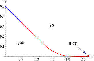
(a) D3/D5

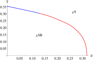
(b) D3/D7

Figure 1: $T$-$d$ phase diagrams at ${{B}}=1$ for the $D5$ (a) and $D7$ (b) probes. The red lines correspond to second order phase transitions and the blue to first order phase transitions. There is an isolated BKT phase transition in the $D5$-brane case at exactly $T=0$ due to the competition between ${{B}}$ and $d$ which in $2+1$ dimensions have the same scaling dimension. The BKT phase transition is absent in the $D7$ case because the dimensions are $[d]=3$ and $[{{B}}]=2$ which means that such a competition cannot arise and thus the IR phenomenology is dominated by $d$.

The finite magnetic field increases the binding energy of the fundamental charges and thus stabilizes the mesons, whereas the thermal fluctuations at finite temperature act to destabilize them. The finite charge density means that one can never have fully stable bound states and thus the width of all mesonic fluctuations is finite. The transition is thus not a meson melting phase transition (as is the case at zero baryon density) but a chiral symmetry breaking phase transition. For large baryon densities or temperatures, the embedding is always the trivial embedding but the transition from the trivial to the non-trivial embedding may be first order or second order in the $D7$-brane case, with the addition of a BKT phase transition at $T=0$ in the $D5$ brane case. This has already been discussed extensively in [22, 23, 24].

3.2 The phase diagram with finite $E$ and $B$

The inclusion of both finite electric and magnetic field has been discussed previously in [25] however in that case the electric and magnetic fields were parallel and thus there was no Hall current. In the current paper we study the case where the two are perpendicular, giving a very different phenomenology and a somewhat different phase structure. In the following sections we will deal with various slices in the finite $E$ part of the phase diagram.

The phenomenology of branes with finite electric fields has been covered extensively in [31, 14, 32] and in [27] the interpretation of an open-string horizon with a membrane interpretation was elucidated.

3.2.1 Transition on the $E$-axis: $T=d=0$

In section 3.1 we discussed the $T$-$d$ phase diagram. By looking at the behaviour on the $E$-axis (again, at finite, fixed ${{B}}$), that is at $T=d=0$ we can get an idea of the full $3D$ phase structure. Taking the $T=d=0$ case of the Legendre transformed Lagrangian,(2.12), and specializing to the $E$-axis we get the simplified Lagrangian:

$$L_{\mathrm{LT}}=\rho^{(q-1)/2}\sqrt{\left(1+\frac{1-{{E}}^{2}}{(\rho^{2}+L^{2})^{2}}\right)}\sqrt{(1+L^{\prime 2})}\ ,$$ (3.1)

where we are restricting to the case where ${{E}}<1$ (i.e. ${{E}}<{{B}}$) such that there is no singular shell and no current induced (2.22). For ${{E}}>1$ the embedding is always flat and thus there is no condensate whereas for ${{E}}<1$ there is a finite condensate which vanishes as ${{E}}\rightarrow 1$.

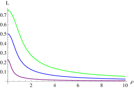
(a) Embeddings with $m=0$. Colors match large dots of (b).

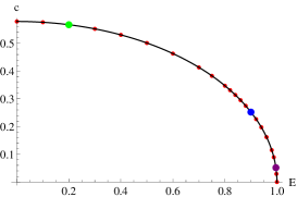
(b) $c$ vs $E$. Red dots are numerical values and the back curve is $c=0.58(1-E^{2})^{1/2}$

Figure 2: Second order phase transition for the $D3/D5$ system with $B=1$ varying $E$ at $T=d=0$.

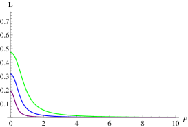
(a) Embeddings with $m=0$. Colors match large dots of (b).

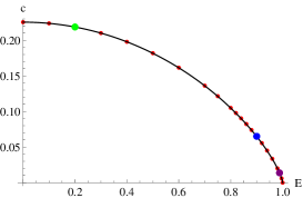
(b) $c$ vs $E$. Red dots are numerical values and the back curve is $c=0.225(1-E^{2})^{3/4}$

Figure 3: Second order phase transition for the $D3/D7$ system with $B=1$ varying $E$ at $T=d=0$.

In this case the critical exponent of the system can be computed analytically. If we substitute $1-{{E}}^{2}$ for $\mathbb{B}$, then the actions are identical to the case at finite $\mathbb{B}$ and $T={{E}}=0$ formally. This is nothing but a Lorentz transformation. On dimensional grounds the condensate must be related to the electric field as:

$$c\sim({{E}}_{c}-{{E}})^{(q-1)/8}\,.$$ (3.2)

The proportionality constant is determined by numerical analysis at any one point of $\mathbb{B}$. They turn out to be

$$c=0.580(1-{{E}}^{2})^{1/2}\qquad(D5)\ ,$$ (3.3)

$$c=0.225(1-{{E}}^{2})^{3/4}\qquad(D7)\,,$$ (3.4)

where ${{E}}_{c}=1$. The $D3/D5$ system has the mean-field exponent $1/2$, while that of the $D3/D7$ shows the non-mean-field exponent 3/4. This is in agreement with the Ohm currents (2.23) and (2.25) which are also understood on dimensional grounds.

We are able to check our numerical procedures against the analytic results and this is shown in Fig 2 and Fig 3. In each of these plots, $(a)$ shows the embedding configuration for a number of different values of the electric field strength, ${{E}}$, while $(b)$ gives a plot of the condensate as a function of ${{E}}$ going from 0 to 1. The large coloured dots in the $(b)$ plots correspond to the three embedding configurations in $(a)$. The black curves ((3.3) and (3.4)) agree with the red dots, which are numerical values obtained for various ${{E}}$.

3.2.2 $T-E$ plane

The Lagrangian (2.12) with $d=0$ is rather complicated and not terribly illuminating so we don’t present it in full here. Both electric field and finite temperature act to destabilize the fluctuations of the fundamental bilinear operator. The critical line in the $T-E$ plane, shown in Fig 4, corresponds to a first order phase transition between a chirally symmetric phase and a chiral symmetry broken phase. This first order transition becomes a second order transition at T=0 which is of mean field type in the $D5$ case and a non-mean field transition (with critical exponent $3/4$) in the $D7$ case.

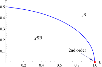
(a) D3/D5. the critical exponent at T=0 is $1/2$

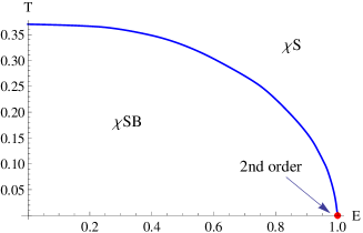
(b) D3/D7. the critical exponent at T=0 is $3/4$

Figure 4: $T$-$E$ phase diagram at $B=1$ and $d=0$. All fist order transitions(blue) except one second order point(red) at $T=0$

3.2.3 $d-E$ plane

At zero temperature the Lagrangian (2.12) simplifies greatly, with the currents given in (2.19).

$$\mbox{${\cal L}$}_{LT}=\sqrt{d^{2}\left(1-\frac{{{E}}^{2}}{{{B}}^{2}}\right)+\rho^{q-1}\left(1+\frac{{{B}}^{2}-{{E}}^{2}}{(\rho^{2}+L^{2})^{2}}\right)}\sqrt{1+L^{\prime 2}}\,.$$ (3.5)

Although the Lagrangian is simplified, the numerics at $T=0$ are somewhat more complicated than the finite temperature case. At $T=0$ we are not able to integrate the equations of motion from the IR at $r=0$ and instead have to solve from the UV. At finite temperature the singular nature of the equation of motion at the horizon means that given a single boundary condition plus the condition of regularity we can shoot out to the UV and pick off the solution which has zero mass. Shooting from the UV into the IR however we choose the zero mass solution and then have to find the value of the condensate such that the brane embedding hits the point $r=0$. Because of the singular nature of the equation of motion at this point, the numerics are somewhat sensitive to the accuracy which we require. The second subtlety is that because there are actually an infinity of solutions which hit the singularity (associated with the self-similar spiral structure in the $c-m$ plane, [8]) we must be careful that we pick the one associated with the lowest free energy.

Having tamed the numerics we are able to study the phase transition from the chirally symmetric phase to the chiral symmetry breaking phase and this is plotted in Fig 5.

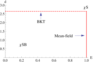
(a) D3/D5. The dotted line is a BKT transition and the solid line is mean-field 2nd order transition.

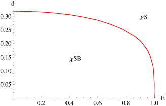
(b) D3/D7. All mean field 2nd order except one point ($d=0,E=1$).

Figure 5: The $d$-$E$ phase diagram for the $D5$ (left) and $D7$ (right) systems. Chiral symmetry is broken inside the enclosed region. $B=1$ and $T=0$.

For the $D5$ case the analysis of the condensate as a function of $d$ and $E$ is shown in Fig 6.

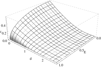
(a) $c(E,d)$. BKT transitions on the line $d=\sqrt{7}$ for ($0\leq E<1$). Mean field second order transition on the line $E=1$ for ($0<d<\sqrt{7}$).

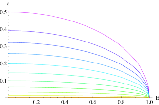
(b) $c$ vs $d$ cross section for a fixed $d$. The critical exponent is $0.5\pm 0.0001$ near phase transition point $E=1$ .

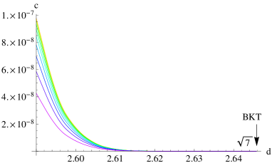
(c) $c$ vs $d$ cross-section near phase transition $d=\sqrt{7}$ for a fixed $E$. $E=0.1,0.2,\cdots,0.9$ from orange to purple. BKT scalings are shown. the BKT transition point $d_{c}=\sqrt{7}$ is independent of $E$ as shown with the IR analysis.

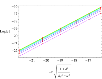
(d) Numerical confirmation of BKT scaling. $c\sim e^{-\pi\sqrt{\frac{1+d^{2}}{d_{c}^{2}-d^{2}}}}$. The slopes are $1\pm 0.001$.

Figure 6: The analysis of the BKT and mean field phase transition for the $D3/D5$ system. $B=1$ and $T=0$.

The phase transition as $d$ is increased is independent of the size of the electric field (for ${{E}}<1$) and is of BKT type. As ${{E}}$ increases for $d<d_{c}=\sqrt{7}$ the phase transition is of mean field type and again its position is independent of the value of $d$. This should be contrasted with the $D7$ system where the second order phase transition takes a non-trivial profile in the $d-E$ plane. The $D7$-brane analysis is relatively simple and so is not presented here.

The line of BKT transitions in the $D3/D5$ system and its ${{E}}$-independence can be understood from the IR dynamics. After scaling all quantities by ${{B}}$ we have the embedding Lagrangian, at small $\rho$,

$$\mbox{${\cal L}$}_{LT}\sim\sqrt{1-{{E}}^{2}}\sqrt{d^{2}+\rho^{4}{(\rho^{2}+L^{2})^{2}}}\sqrt{1+L^{\prime 2}}\,.$$ (3.6)

Note that the ${{E}}$ part is factored out from the Legendre transformed action so that the dynamics is identical to the ${{E}}=0$ case. The slipping mode for a small fluctuation of the embedding $L$ in the IR $\rho\ll(1,d)$ behaves as a scalar in AdS₂ space with mass $-\frac{2}{1+d^{2}}$. The Breitenlohner-Freedman (BF) bound for a scalar in AdS₂ is $-1/4$, so below $d=\sqrt{7}$ the BF bound is violated and the phase transition to a broken symmetry phase occurs. Note that we get a good fit for the whole of the region close to the phase transition with $c\sim 2.6e^{\frac{-\pi\sqrt{1+d^{2}}}{\sqrt{7-d^{2}}}}\sqrt{1-{{E}}}$. The exponent comes from the analytic calculation given in [22].

3.3 $T$-$d$-$E$ phase diagram

Finally, in Fig 7 we combine the above information with the phase structure outside the two dimensional slices we have analyzed above. The critical point linking the first and second order phase transitions give a line on the surface of the phase transition face. This links surfaces of second order and first order phase transitions. The line of BKT phase transitions is an isolated region in the $D3/D5$ diagram and the rest of the diagram is either of mean-field second order type or of first order type. Fig 7 summarizes our full analysis.

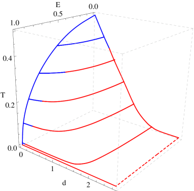
(a) D3/D5

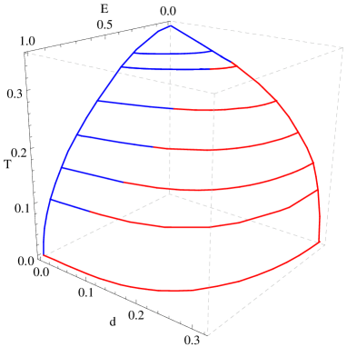
(b) D3/D7

Figure 7: 3D phase diagram of D3/D7 and D3/D5 system at $B=1$ as a function of $T$,$d$, and $E$.

4 Summary

We have studied the D3/D7 and D3/D5 systems in the presence of mutually perpendicular electric and magnetic fields to deduce the temperature and density phase structure of the dual gauge theories. Those theories are the 3+1 dimensional ${\cal N}=4$ super Yang Mills theory with quark hypermultiplets introduced in all field theory directions and on a 2+1 dimensional defect respectively. The full results are displayed, for constant magnetic field, in Fig 7. There are two phases. At large $d,T,E$ the theory is in a chirally symmetric phase, while at low $d,T,E$ the phase displays chiral symmetry breaking through a non-zero quark condensate. In the gravity description these transitions are associated with embeddings of the probe D7 or D5-brane that either lie flat (the symmetric phase) or are given by non-trivial profiles in the holographic directions breaking the symmetry.

At zero temperature the phase transition is continuous for both D3/D7 and D3/D5 systems. However, the D3/D5 system has a special feature that there is a holographic BKT transition for low $E$ field values. In this regime the deep IR is dominated by both the magnetic field and density regardless of $E$. When the electric field becomes sufficiently large to trigger the transition on its own the transition becomes second order and mean field. At intermediate temperature, at low density the transition is first order whilst at high density it is mean-field second order. The critical lines between these regimes can be inferred from the Fig 7. At high temperature the transition becomes all first order.

If we were to include finite mass, the structure may have even more subtleties within. The more features we can find in our phase diagrams, the more chance there is we can link such basic holographic models with real world systems. We leave the extensions of this phase space for future work.

References

- [1] J. Erdmenger, N. Evans, I. Kirsch, and E. Threlfall, Mesons in Gauge/Gravity Duals - A Review, Eur. Phys. J. A35 (2008) 81–133, [arXiv:0711.4467].
- [2] J. M. Maldacena, The Large N limit of superconformal field theories and supergravity, Adv.Theor.Math.Phys. 2 (1998) 231–252, [hep-th/9711200].
- [3] S. S. Gubser, I. R. Klebanov, and A. M. Polyakov, Gauge theory correlators from non-critical string theory, Phys. Lett. B428 (1998) 105–114, [hep-th/9802109].
- [4] E. Witten, Anti-de Sitter space and holography, Adv. Theor. Math. Phys. 2 (1998) 253–291, [hep-th/9802150].
- [5] M. Grana and J. Polchinski, Gauge / gravity duals with holomorphic dilaton, Phys. Rev. D65 (2002) 126005, [hep-th/0106014].
- [6] M. Bertolini, P. Di Vecchia, M. Frau, A. Lerda, and R. Marotta, N = 2 gauge theories on systems of fractional D3/D7 branes, Nucl. Phys. B621 (2002) 157–178, [hep-th/0107057].
- [7] A. Karch and E. Katz, Adding flavor to AdS/CFT, JHEP 06 (2002) 043, [hep-th/0205236].
- [8] V. G. Filev, C. V. Johnson, R. C. Rashkov, and K. S. Viswanathan, Flavoured large N gauge theory in an external magnetic field, JHEP 10 (2007) 019, [hep-th/0701001].
- [9] S. Nakamura, Y. Seo, S.-J. Sin, and K. P. Yogendran, A new phase at finite quark density from AdS/CFT, J. Korean Phys. Soc. 52 (2008) 1734–1739, [hep-th/0611021].
- [10] S. Kobayashi, D. Mateos, S. Matsuura, R. C. Myers, and R. M. Thomson, Holographic phase transitions at finite baryon density, JHEP 02 (2007) 016, [hep-th/0611099].
- [11] K.-Y. Kim, S.-J. Sin, and I. Zahed, Dense hadronic matter in holographic QCD, hep-th/0608046.
- [12] K.-Y. Kim, S.-J. Sin, and I. Zahed, The Chiral Model of Sakai-Sugimoto at Finite Baryon Density, JHEP 01 (2008) 002, [arXiv:0708.1469].
- [13] T. Albash, V. G. Filev, C. V. Johnson, and A. Kundu, Finite Temperature Large N Gauge Theory with Quarks in an External Magnetic Field, JHEP 07 (2008) 080, [arXiv:0709.1547].
- [14] J. Erdmenger, R. Meyer, and J. P. Shock, AdS/CFT with Flavour in Electric and Magnetic Kalb-Ramond Fields, JHEP 12 (2007) 091, [arXiv:0709.1551].
- [15] N. Evans, A. Gebauer, K.-Y. Kim, and M. Magou, Holographic Description of the Phase Diagram of a Chiral Symmetry Breaking Gauge Theory, JHEP 03 (2010) 132, [arXiv:1002.1885].
- [16] K. Jensen, A. Karch, and E. G. Thompson, A Holographic Quantum Critical Point at Finite Magnetic Field and Finite Density, JHEP 05 (2010) 015, [arXiv:1002.2447].
- [17] B. Gwak, M. Kim, B.-H. Lee, Y. Seo, and S.-J. Sin, Phases of a holographic QCD with gluon condensation at finite Temperature and Density, arXiv:1105.2872.
- [18] A. Karch and L. Randall, Open and closed string interpretation of SUSY CFT’s on branes with boundaries, JHEP 06 (2001) 063, [hep-th/0105132].
- [19] O. DeWolfe, D. Z. Freedman, and H. Ooguri, Holography and defect conformal field theories, Phys. Rev. D66 (2002) 025009, [hep-th/0111135].
- [20] J. Erdmenger, Z. Guralnik, and I. Kirsch, Four-Dimensional Superconformal Theories with Interacting Boundaries or Defects, Phys. Rev. D66 (2002) 025020, [hep-th/0203020].
- [21] R. C. Myers and M. C. Wapler, Transport Properties of Holographic Defects, JHEP 0812 (2008) 115, [arXiv:0811.0480].
- [22] K. Jensen, A. Karch, D. T. Son, and E. G. Thompson, Holographic Berezinskii-Kosterlitz-Thouless Transitions, Phys. Rev. Lett. 105 (2010) 041601, [arXiv:1002.3159].
- [23] N. Evans, A. Gebauer, K.-Y. Kim, and M. Magou, Phase diagram of the D3/D5 system in a magnetic field and a BKT transition, Phys. Lett. B698 (2011) 91–95, [arXiv:1003.2694].
- [24] N. Evans, K. Jensen, and K.-Y. Kim, Non Mean-Field Quantum Critical Points from Holography, Phys. Rev. D82 (2010) 105012, [arXiv:1008.1889].
- [25] N. Evans, A. Gebauer, and K.-Y. Kim, Phase Structure of the D3/D7 Holographic Dual, JHEP 05 (2011) 067, [arXiv:1103.5627].
- [26] A. O’Bannon, Hall Conductivity of Flavor Fields from AdS/CFT, Phys. Rev. D76 (2007) 086007, [arXiv:0708.1994].
- [27] K.-Y. Kim, J. P. Shock, and J. Tarrio, The open string membrane paradigm with external electromagnetic fields, arXiv:1103.4581.
- [28] J. Babington, J. Erdmenger, N. J. Evans, Z. Guralnik, and I. Kirsch, Chiral symmetry breaking and pions in non-supersymmetric gauge / gravity duals, Phys. Rev. D69 (2004) 066007, [hep-th/0306018].
- [29] J. Erdmenger, V. Grass, P. Kerner, and T. H. Ngo, Holographic Superfluidity in Imbalanced Mixtures, arXiv:1103.4145. * Temporary entry *.
- [30] J. Mas, J. P. Shock, and J. Tarrio, Holographic Spectral Functions in Metallic AdS/CFT, JHEP 09 (2009) 032, [arXiv:0904.3905].
- [31] A. Karch and A. O’Bannon, Metallic AdS/CFT, JHEP 09 (2007) 024, [arXiv:0705.3870].
- [32] T. Albash, V. G. Filev, C. V. Johnson, and A. Kundu, Quarks in an External Electric Field in Finite Temperature Large N Gauge Theory, JHEP 08 (2008) 092, [arXiv:0709.1554].