An improvement of the Molière -Fano multiple
scattering theory

Abstract

In the framework of unitary Glauber approximation for particle-atom scattering, we develop the general formalism of the Molière–Fano multiple scattering theory (M–F theory) on the basis of reconstruction of the generalized optical theorem in it. We present rigorous relations between some exact and first-order parameters of the Molière multiple scattering theory, instead of the approximate one obtained in the original paper by Molière. We consider the relative unitarity corrections and the Coulomb corrections to the quantities of the M–F theory. Also, we examine their $Z$ dependence in the range of nuclear charge from $Z=4$ to $Z=92$. Additionally, we show the difference between our results and those of Molière over this range of $Z$.

Joint Institute for Nuclear Research, 141980 Dubna, Russia

1 Introduction

The Molière–Fano multiple scattering theory of charged particles [1–3] is the most used tool for taking into account the multiple scattering effects in experimental data processing. The experiment DIRAC [4]and many others ([5], MuScat [6], MUCOOL [7] experiments, etc.) face the problem of excluding the multiple scattering effects in matter from obtained data.

The standard theory of multiple scattering [4, 5, 6] proposed by Molière [1, 2] and Fano [3] and some its modifications [6–11] are used for this aim. The modifications, developed in [6–8], are motivated by experiments [6, 7]; they are connected with including analogues of the Fano corrections in the Molière theory and determining their range of applicability [6–9]. In [10] a modified transport equation is presented whose solution is applicable over the range of angles, from $0$ to $180^{\circ}$. In [11] results of experiments [12] are qualitatively explained within the framework of the theory allowing for pair correlations in the spatial distribution of scatterers.

Estimation of the theory accuracy is of particular importance for the DIRAC experiment because it’s high angular resolution. One possible source of the M–F theory inaccuracy is use in [1–3] an approximate expression for the target-elastic particle-atom scattering amplitude which violates the generalized optical theorem

$$\Im f_{el}(0)=\frac{k}{4\pi}\sigma_{tot}=\frac{k}{4\pi}(\sigma_{el}+\sigma_{in})$$ (1)

or, in other words, unitarity condition. Another possible source of inaccuracy is using in calculations an approximate relation for the exact and the Born values of the screening angle ($\chi_{a}^{\,\prime}$)

$$\chi_{a}^{\,\prime}\approx\big{(}\chi_{a}^{\,\prime}\big{)}^{\scriptscriptstyle B}\sqrt{1+3.34\left(Z\alpha\right)^{2}}$$ (2)

obtained in the original paper by Molière [1]. Therefore, the problem of estimating the M–F theory accuracy and its improvement becomes important.

In this work, we obtain the relative unitarity corrections to the parameters of the Molière–Fano theory both analytically and numerically resulting from a reconstruction of the unitarity in the particle-atom scattering theory, and we found that they are of an order of $Z\alpha^{2}$. Also, we consider the analytical and numerical results for the Coulomb corrections to the parameters of the Molière theory, and we show that these corrections can be numerically large, e.g., about $40\div 50\%$ for $Z=92$. Additionally, we demonstrate the difference between our results and those of Molière over the range $4\leq Z\leq 92$.

The paper is organized as follows. In Section 2, we consider the approximations of the M–F theory. In Section 3, we obtain the analytical and numerical results for the unitarity corrections and the Coulomb corrections to the parameters of the M–F theory. In Conclusion, we briefly summarize our results.

2 Approximations of the M–F theory

2.1 Small-angle approximation

Let all scattering angles are small $\theta\ll 1$ so that $\sin\theta\sim\theta$, and the scattering problem is equivalent to diffusion in the plane of $\theta$. Now let $\sigma_{el}(\chi)$ be the elastic differential cross section for the single scattering into the angular interval $\vec{\chi}=\vec{\theta}-\vec{\theta}^{\prime}$, and $W_{\scriptscriptstyle M}(\theta,t)\theta d\theta$ is the number of scattered particles in the interval $d\theta$ after traversing a target thickness $t$. Then, within the small-angle approximation, the transport equation for the distribution function $W_{\scriptscriptstyle M}(\theta,t)$ reads

$$\frac{\partial W_{\scriptscriptstyle M}(\theta,t)}{\partial t}=-n_{0}W_{\scriptscriptstyle M}(\theta,t)\int\sigma_{el}(\chi)d^{2}\chi+n_{0}\int W_{\scriptscriptstyle M}(\vec{\theta}-\vec{\chi},t)\sigma_{el}(\chi)d^{2}\chi,$$ (3)

where $n_{0}$ is the density of the scattering centers per unit volume, $d^{2}\chi=\chi d\chi d\phi/(2\pi)$, and $\phi$ denotes the azimuthal angle of the vector $\vec{\chi}=(\theta,\phi)$.

Introducing the Bessel transformation of distribution

$$g(\eta,t)=\int\limits_{0}^{\infty}\theta J_{0}(\eta\theta)W_{\scriptscriptstyle M}(\theta,t)d\theta\ ,$$ (4)

$$W_{\scriptscriptstyle M}(\theta,t)=\int\limits_{0}^{\infty}\eta J_{0}(\eta\theta)g(\eta,t)d\eta\ ,$$ (5)

and using the folding theorem (see details in Appendix), we obtain the transport equation for the Bessel-transformed function $g(\eta,t)$:

$$\frac{\partial g(\eta,t)}{\partial t}=-n_{0}\,g(\eta,t)\int\limits_{0}^{\infty}\sigma_{el}(\chi)\chi d\chi[1-J_{0}(\eta\chi)]\ ,$$ (6)

whose solution is

$$g(\eta,t)=\exp\left\{N(\eta,t)-N_{0}(0,t)\right\}\ ,$$ (7)

$$N(\eta,t)=n_{0}\,t\int\sigma_{el}(\chi)\chi d\chi J_{0}(\eta\chi)\ .$$ (8)

Inserting this solution back in (5), we get

$$W_{\scriptscriptstyle M}(\theta,t)=\int\limits_{0}^{\infty}\eta d\eta J_{0}(\eta\theta)\exp\left\{-n_{0}\,t\,\int\limits_{0}^{\infty}\sigma_{el}(\chi)\chi d\chi\left[1-J_{0}(\eta\chi)\right]\right\}.$$ (9)

This equation is exact for any scattering law, provided only the angles are small compared with a radian.

2.2 Approximate solution of the transport equation

For the screening potential, the scattering cross section reads

$$\sigma_{el}(\chi) = \frac{4Z^{2}e^{4}}{(vp)^{2}(\chi^{2}+\chi_{0}^{2})^{2}},$$ (10)

$$\chi_{0}=\frac{\lambda}{a}\,,\quad\lambda=\frac{\hbar}{mv}\,,\quad a=0.885\,a_{0}Z^{-1/3}\,,\quad a_{0}=\frac{\hbar}{p\alpha},$$ (11)

where $a$ is the Fermi radius of the atom, $a_{0}$ presents the Bohr radius of the particle, $p=mv$ and $v$ are the incident particle momentum and the particle velocity in the laboratory frame, correspondingly, and $\alpha=1/137$ denotes the fine structure constant.

Let us write

$$n_{0}t\,\sigma_{el}(\chi)\chi d\chi=2\chi_{c}^{2}\chi d\chi\frac{q_{el}(\chi)}{\chi^{4}},\qquad 2\chi_{c}^{2}=4\pi n_{0}t\frac{Z^{2}e^{4}}{(pv)^{2}},$$ (12)

where $q_{el}(\chi)$ is the ratio of the actual scattering cross section to the Rutherford one, and $\chi_{c}$ is the so-called ‘characteristic angle’

$$\chi_{c}^{2}=4\pi n_{0}t\left(\frac{Z\alpha}{\beta p}\right)^{2},$$ (13)

whose physical meaning is that the probability of scattering on the angles exceeding $\chi_{c}$ is unity.

In terms of $\chi_{c}$ and $q_{el}$, the solution of (6) becomes

$$-\ln g(\eta,t)=2\,\chi_{c}^{2}\int\limits_{0}^{\infty}\frac{d\chi}{\chi^{3}}\,q_{el}(\chi)\left[1-J_{0}(\chi\eta)\right].$$ (14)

Estimating the value of the latter integral and introducing the notion of the screening angle $\chi_{a}$

$$-\ln\chi_{a}=\lim_{\varsigma\to\infty}\left[\int\limits_{0}^{\varsigma}\frac{d\chi}{\chi}\,q_{el}(\chi)+\frac{1}{2}-\ln\varsigma\right],$$ (15)

where $\chi_{0}\ll\varsigma\ll\chi_{c}$, we obtain for the Bessel-transformed distribution function $g(\eta,t)$ the expression

$$-\ln g(\eta,t)=\frac{1}{2}(\chi_{c}\eta)^{2}\left[-\ln(\chi_{a}\eta)+\frac{1}{2}+\ln 2-C_{\scriptscriptstyle E}\right].$$ (16)

Here, $C_{\scriptscriptstyle E}=0.5772\ldots$ is the Euler constant. Then introducing the new variables $y=\chi_{c}\eta$ and $\theta/\chi_{c}=u$, as a result, we get

$$-\ln g(\eta,t)=\frac{1}{4}y^{2}\left[b_{el}-\ln\left(\frac{1}{4}y^{2}\right)\right],$$

(17)

$$b_{el}=\ln\frac{\chi_{c}^{2}}{\chi_{a}^{2}}+1-2C_{\scriptscriptstyle E}\equiv\ln\frac{\chi_{c}^{2}}{(\chi^{\prime}_{a})^{2}},$$ (18)

and Molière’s transformed equation becomes

$$W_{\scriptscriptstyle M}(\theta)\theta d\theta=udu\int\limits_{0}^{\infty}ydyJ_{0}(uy)\exp\left\{-\frac{y^{2}}{4}\left[b_{el}-\ln\left(\frac{y^{2}}{4}\right)\right]\right\}.$$ (19)

This rather simple formula permits one to develop an iteration procedure for $W(\theta)$. Really, putting

$$b_{el}=B-\ln B,$$ (20)

we can write the angular distribution function as

$$W_{\scriptscriptstyle M}(\theta,B) = \frac{1}{\overline{\theta^{\,2}}}\int\limits_{0}^{\infty}ydyJ_{0}(\theta y)e^{-y^{2}/4}\exp\left[\frac{y^{2}}{4B}\ln\left(\frac{y^{2}}{4}\right)\right],$$ (21)

with $\overline{\theta^{\,2}}=\chi_{c}^{2}B$. Introducing the variable $x=u^{2}/B$, one can obtain the expansion of the distribution function in a power series in $1/B$:

$$W_{\scriptscriptstyle M}(\theta,B)\theta d\theta = \frac{1}{\overline{\theta^{\,2}}}\theta d\theta\left[W^{(0)}(x)+\frac{1}{B}W^{(1)}(x)+\frac{1}{B^{2}}W^{(2)}(x)+\ldots\right],$$ (22)

in which

$$W^{(0)}(x)=\frac{2}{\overline{\theta^{\,2}}}\exp\left(\!\!-\frac{\theta^{2}}{\overline{\theta^{\,2}}}\right),\quad\ldots\;,\quad W^{(n)}(x)=\frac{1}{\overline{\theta^{\,2}}}\int\limits_{0}^{\infty}ydyJ_{0}\left(\frac{\theta}{\bar{\theta}}\,y\right)e^{-y^{2}/4}\left[\frac{y^{2}}{4}\ln\left(\frac{y^{2}}{4}\right)\right]^{n}.$$ (23)

The result of numerical integration $W^{(n)}(x)$ was obtained in papers by Molière, Bethe and Scott [1, 13, 14]. In practice, the value of the solution of the transcendental equation (20) is large enough to provide the convergence of the expansion series, i.e., $4.5\leq B\leq 20$.

2.3 Born approximation

On the one hand, Molière writes the elastic Born cross section for fast charged particle Coulomb scattering as follows:

$$\sigma_{el}^{\scriptscriptstyle B}(\chi)=\sigma_{el}^{\scriptscriptstyle R}(\chi)\,\,q_{el}^{\scriptscriptstyle B}(\chi).$$ (24)

For angles $\chi$ small compared with a radian, the Rutherford cross section has a simple approximation, and (24) yields

$$\sigma_{el}^{\scriptscriptstyle B}(\chi) = \frac{\chi_{c}^{2}}{4\pi n_{0}t(1-\cos\chi)^{2}}\,\,q_{el}^{\scriptscriptstyle B}(\chi)$$ (25)

$$\approx \frac{\chi_{c}^{2}}{\pi n_{0}t\,\chi^{4}}\,\,q_{el}^{\scriptscriptstyle B}(\chi).$$ (26)

Molière represents the Born screening angle $\chi_{a}^{\scriptscriptstyle B}$ via $q_{el}^{\,\scriptscriptstyle B}(\chi)$ by the equation

$$-\ln\big{(}\chi^{\scriptscriptstyle B}_{a}\big{)} = \lim\limits_{\varsigma\rightarrow\infty}\left[\int\limits_{0}^{\varsigma}\frac{q_{el}^{\,\scriptscriptstyle B}(\chi)d\chi}{\chi}+\frac{1}{2}-\ln\varsigma\right]$$ (27)

with

$$\chi_{0}\ll\varsigma\ll 1/\eta\sim\chi_{c}$$ (28)

and $\chi_{0}\sim m_{e}\alpha Z^{1/3}/p$.

When the Born parameter $a$ is equal to zero, (27) can be evaluated directly using the facts that $q(0)=0$ and $\lim\limits_{\varsigma\rightarrow\infty}q(\varsigma)=1$. Then the following approximation can be obtained for $\big{(}\chi_{a}^{\,\prime}\big{)}^{\scriptscriptstyle B}$:

$$\big{(}\chi_{a}^{\,\prime}\big{)}^{\scriptscriptstyle B}=\left[\exp(C_{\scriptscriptstyle E}-0.5)\right]\,\frac{\lambda}{p}\,\,1.065=\sqrt{1.174}\,\,\,\chi_{0}\,\sqrt{1.13},$$ (29)

where $\lambda=m_{e}\alpha Z^{1/3}/0.885$.

On the other hand, Molière writes the non-relativistic Born cross section in the form

$$\sigma_{el}^{\scriptscriptstyle B}(\chi)=k^{2}\left|\int\limits_{0}^{\infty}\rho\,d\rho J_{0}\left(2k\rho\,\sin\frac{\chi}{2}\right)\Phi_{\scriptscriptstyle M}^{\scriptscriptstyle B}(\vec{\rho})\right|^{2},$$ (30)

in which the Born phase shift is given by

$$\Phi_{\scriptscriptstyle M}^{\scriptscriptstyle B}(\vec{\rho})=-\frac{2}{v}\int\limits_{\rho}^{\infty}\frac{U_{\lambda}(r)rdr}{\sqrt{r^{2}-\rho^{2}}}=-\frac{1}{v}\int\limits_{-\infty}^{\infty}U_{\lambda}\left(r=\sqrt{\rho^{2}+z^{2}}\right)dz$$ (31)

in units of $\hbar=c=1$ Here, $k$ is the wave number of the incident particle, the variable $\rho$ corresponds to the impact parameter of the collision, and $U_{\lambda}(r)$ is a screened Coulomb potential of the target atom.

The Born target-elastic single cross section satisfies the following relations:

$$\frac{d\sigma^{B}_{el}}{d\Omega}=|f_{el}(\theta)|^{2},$$ (32)

$$\Im f_{el}(0) = \frac{k}{4\pi}\sigma^{B}_{el}\neq\frac{k}{4\pi}\sigma^{B}_{tot}.$$ (33)

The Born approximation result for the target-elastic scattering amplitude $f_{el}$ with the momentum transfer $q=k\theta$ reads

$$f_{el}(\theta)=ik\int\limits_{0}^{\infty}J_{0}(\rho\,q)[1-e^{i\Phi_{\scriptscriptstyle M}(\vec{\rho})}]\rho\,d\rho.$$ (34)

2.4 Approximate relation between the quantities $\chi_{a}$ and $\chi_{a}^{\scriptscriptstyle B}$

For actual determining the screening angle

$$-\ln\big{(}\chi_{a}\big{)} = \lim\limits_{\varsigma\rightarrow\infty}\left[\int\limits_{0}^{\varsigma}\left(1-\frac{F_{\scriptscriptstyle A}(p\chi)}{Z}\right)^{2}\frac{d\chi}{\chi}+\frac{1}{2}-\ln\varsigma\right]$$ (35)

$$= \lim\limits_{\varsigma\rightarrow\infty}\left[\int\limits_{0}^{\varsigma}\frac{q_{el}(\chi)d\chi}{\chi}+\frac{1}{2}-\ln\varsigma\right]$$ (36)

via the Thomas–Fermi form factor $F_{\scriptscriptstyle T-F}(q)$

$$F_{\scriptscriptstyle T-F}(q)^{\scriptscriptstyle M}=\sum\limits_{i=1}^{3}\frac{c_{i}\lambda_{i}^{2}}{q^{2}+\lambda_{i}^{2}}\,,$$ (37)

where

$$c_{1}=0.35,\quad c_{2}=0.55,\quad c_{3}=0.10,$$

$$\lambda_{1}=0.30\lambda,\quad\lambda_{2}=4\lambda_{1},\quad\lambda_{3}=5\lambda_{2},$$

which does not make use of the Born approximation, Molière uses the WKB method.

He starts with the exact formulas for the WKB differential cross section $\sigma_{el}(\chi)$ and the corresponding ratio $q_{el}(\chi)$

$$\sigma_{el}(\chi)=k^{2}\left|\int\limits_{0}^{\infty}\rho\,d\rho\,J_{0}(k\chi\rho)\bigg{\{}1-\exp\big{[}i\Phi_{\scriptscriptstyle M}(\vec{\rho})\big{]}\bigg{\}}\right|^{2},$$ (38)

$$q_{\,el}(\chi)=\frac{(k\chi)^{4}}{4\,a^{2}}\left|\int\limits_{0}^{\infty}\rho\,d\rho J_{0}(k\chi\rho)\bigg{\{}1-\exp\big{[}i\Phi_{\scriptscriptstyle M}(\vec{\rho})\big{]}\bigg{\}}\right|^{2},$$ (39)

but evaluates these quantities only approximately.

For estimation of (39), Molière uses the Born shift (31) with the potential

$$U_{\lambda}(r)=\pm Z\,\frac{\alpha}{r}\,\Lambda(\lambda r)$$ (40)

and the Thomas–Fermi (T–F) screening function, which Molière approximates by a sum of three exponentials

$$\Lambda(\lambda r) \simeq 0.1e^{-6\,\lambda r}+0.55e^{-1.2\,\lambda r}+0.35e^{-0.3\,\lambda r}.$$ (41)

Here, $r_{sc}=0.885/m_{e}\alpha Z^{1/3}$ is the T–F radius.

This is good only to terms of first order in the Born parameter $a$. Neglecting terms of orders higher than $a^{2}$ in the obtained result, he get the following approximate expression for $q_{el}(\chi)$:

$$q_{\,el}(\chi)\approx 1-\frac{8.85}{(\chi/\chi_{0})^{2}}\bigg{[}1+2.303\,a^{2}\lg\frac{7.2\cdot 10^{-4}(\chi/\chi_{0})^{4}}{\left(a^{4}+a^{2}/3+0.13\right)}\bigg{]},$$ (42)

which is one of the basic expressions of the Molière theory. Estimating $q_{el}(\chi)$ for different $a$ values, Molière devised an interpolation scheme for $(\chi/\chi_{0})^{2}$:

$$(\chi/\chi_{0})^{2}\approx A_{q}+a^{2}B_{q}.$$ (43)

Finally, calculating the screening angle defined by

$$-\ln\big{(}\chi_{a}\big{)}=\frac{1}{2}-\ln\chi_{0}-\int\limits_{0}^{1}dq\ln\left(\frac{\chi}{\chi_{0}}\right)$$ (44)

and assuming a linear relation between $\chi_{a}^{2}$ and $a^{2}$, he get the following interpolating formula for the screening angle:

$$\chi_{a}\approx\chi_{0}\sqrt{1.13+3.76\,a^{2}}.$$ (45)

2.5 Fano approximation

To estimate a contribution of incoherent scattering on atomic electrons, the squared nuclear charge $Z^{2}$ is often replaced with the sum of the squares of the nuclear and electronic charges $Z(Z+1)$ [2, 3, 13, 15] in basic relations for differential cross-section, some parameters of the theory, etc.

This procedure would be accurate if the single-scattering cross sections were the same for nucleus and electrons of target atoms. Besides, the actual cross sections are different at small and large angles. Fano modified the multiple scattering theory taking into account above differences.

For this purpose, Fano separates the elastic and inelastic contributions to the cross section

$$\sigma(\chi)=\sigma_{el}(\chi)+\sigma_{in}(\chi).$$ (46)

For the inelastic components of the single scattering differential cross sections, the Fano approximation reads

$$\frac{d\sigma_{in}}{d\Omega}=\frac{d\sigma^{\scriptscriptstyle B}_{in}}{d\Omega}.$$ (47)

Since the Born single-scattering amplitudes are pure real, the generalized optical theorem cannot be used to calculate the total cross section in the framework of this approximation.

Fano sets the task of comparing the $\sigma^{B}_{in}(\chi)$ contribution to the exponent of the Goudsmit–Saunderson distribution [16]:

$$W(\theta,t)=2\pi\sum_{l}\left(l+\frac{1}{2}\right)P_{l}(\theta)\exp\left\{\!-n_{0}\,t\!\int\!\sigma^{\scriptscriptstyle B}(\chi)\sin\chi d\chi[1-P_{l}(\chi)]\right\}\!,$$ (48)

where $P_{l}$ is the Legendre polynomial. If we replace the sum over $l$ in (48) by an integral over $\eta$, $\left(l+\frac{1}{2}\right)$ by $\eta$, $P_{l}$ by the well-known formula $P_{l}(\theta)=J_{0}\big{(}\left(l+\frac{1}{2}\right)\theta\big{)}$, and $\sin\chi$ by $\chi$, the expression (48) goes over into small-angle distribution Molière’s and Lewis’ distribution (92).

To achieve the mentioned goal in the small-angle approximation, we determine the corresponding expressions for the inelastic cross section

$$\sigma^{\scriptscriptstyle B}_{in}(\chi)=\sigma^{\scriptscriptstyle R}(\chi)\,q_{\,in}^{\scriptscriptstyle B}(\chi)=\frac{\chi_{c}^{2}}{4\pi n_{0}t\,\,Z\,(1-\cos\chi)^{2}}\,\,q_{\,in}^{\scriptscriptstyle B}(\chi)$$ (49)

$$\approx\frac{\chi_{c}^{2}}{\pi n_{0}t\,\,Z\,\chi^{4}}\,\,q_{\,in}^{\scriptscriptstyle B}(\chi)$$ (50)

and the ‘inelastic cut-off angle’ $\chi_{in}^{\scriptscriptstyle B}$

$$-\ln\big{(}\chi^{\scriptscriptstyle B}_{in}\big{)}=\lim\limits_{\varsigma\rightarrow\infty}\left[\int\limits_{0}^{\varsigma}\frac{q_{\,in}^{\scriptscriptstyle B}(\chi)d\chi}{\chi}+\frac{1}{2}-\ln\varsigma\right]$$ (51)

similarly to (25) and (27), in accordance with [8, 13].

Then, using (25) and (49), we rewrite (21) as follows:

$$W_{\scriptscriptstyle M-F}(\Theta,B) = \frac{1}{\overline{\theta^{\,2}}}\int\limits_{0}^{\infty}ydyJ_{0}(\Theta y)e^{-y^{2}/4}\exp\left(Y_{el}+Y_{in}\right)$$ (52)

with

$$Y_{el}=\frac{y^{2}}{4B}\ln\left(\frac{y^{2}}{4}\right),\quad Y_{in}=\frac{2y^{2}}{(Z+1)B}\int\limits_{\varsigma}^{\infty}[1-J_{0}(\Theta)]\Theta^{-3}d\Theta,$$ (53)

where the parameter $B$ is defined by equation

$$B-\ln B=b_{el}+b_{\,in},$$ (54)

in which

$$b_{\,el}=\ln\left(\frac{\chi_{c}}{\chi^{\scriptscriptstyle B}_{a}}\right)^{2}+1-2C_{\scriptscriptstyle E},\quad b_{in}=\frac{1}{Z+1}\ln\left(\frac{\chi^{\scriptscriptstyle B}_{a}}{\chi^{\scriptscriptstyle B}_{in}}\right)^{2}.$$ (55)

Numerical estimation of the quantity $-u_{in}{=}-\ln\left(\chi^{\scriptscriptstyle B}_{in}\right)^{2}$ yields $\left(-u_{in}\right)_{\mathrm{T-F}}$ $=5.8$ for all $Z$ within the T–F model. This value should not vary greatly from one target material to another.

For sufficiently large angles, with use of exact Rutherford formulas (25) and (49), the correct angular distribution $W(\theta,t)$ can be estimated according to the formula

$$W_{corr}(\theta,t)=W(\theta,t)\left[\sigma^{B}_{exact}(\chi)/\sigma^{R}(\chi\right)],$$ (56)

as suggested Bethe and Fano [3, 13].

3 An improvement of the M–F theory

3.1 Glauber approximation

The multiple scattering amplitude can be represented in the Glauber approximation [17] as

$$F_{if}(\vec{q})=\frac{ik}{2\pi}\int d^{2}\rho\,\exp(i\,\vec{q}\vec{b})\,\Gamma_{if}(\vec{\rho}),$$ (57)

where $\Gamma_{if}(\vec{\rho})$ is so-called ‘profile function’.

We can get a general formulation of the problem by considering the scattering of a pointlike projectile on a system of $Z$ constituents with the coordinates $\vec{r}_{1},\,\vec{r}_{2},\ldots\,,\vec{r}_{\scriptscriptstyle Z}$ and the projections on the plane of the impact parameter $\vec{s}_{1},\,\vec{s}_{2},\ldots\,,\vec{s}_{\scriptscriptstyle Z}$. Then the total phase shift can be written as a sum of the form

$$\widetilde{\chi}(\vec{\rho},\vec{x}_{1},\,\vec{x}_{2},\ldots\,,\vec{x}_{\scriptscriptstyle Z})=\sum\limits_{k=1}^{Z}\widetilde{\chi}_{k}(\vec{\rho}-\vec{s}_{k}).$$ (58)

If we introduce the configuration space for the wave functions $\psi_{i}$ and $\psi_{f}$ in the initial $i$ and the final $f$ constituent’s states, the profile function can be presented as

$$\Gamma_{if}(\vec{\rho}) = \int\prod_{k=1}^{Z}d^{3}r_{k}\,\psi_{f}^{\ast}(\{\vec{r}_{k}\})\psi_{i}(\{\vec{r}_{k}\})\Gamma(\vec{\rho},\{\vec{s}_{k}\})$$ (59)

with an interaction operator

$$\Gamma(\vec{\rho},\{\vec{s}_{k}\})=1-\exp[i\Phi(\vec{\rho},\{\vec{s}_{k}\})]$$ (60)

and a phase-shift function

$$\widetilde{\Phi}(\vec{\rho},\{\vec{s}_{k}\})=Z\widetilde{\chi}(\vec{\rho})-\sum_{k=1}^{Z}\widetilde{\chi}(\vec{\rho}-\vec{s}_{k}).$$ (61)

When the interaction is due to a potential $V(\vec{r})$, the phase function $\widetilde{\chi}(\vec{\rho})$ is given by

$$\widetilde{\chi}(\vec{\rho}) = -\,\frac{1}{v}\int\limits_{-\infty}^{\infty}V\left(\sqrt{\rho^{2}+z^{2}}\right)dz$$ (62)

with the potential of an individual constituent’s

$$V(r)=\,\pm\lim\limits_{\lambda\rightarrow 0}\frac{\alpha}{r}\,e^{-\lambda r},\quad\lambda\sim m_{e}\alpha Z^{1/3}.$$ (63)

The multiple-scattering amplitude $F_{if}(\vec{q})$ (57) is normalized by the relations

$$4\pi\Im F_{ii}(0)=\sigma(i)_{tot},\quad|F_{if}(\vec{q})|^{2}=d\sigma_{if}/dq_{\scriptscriptstyle T},$$ (64)

where

$$\sigma(i)_{tot}=\sigma(i)_{el}+\sigma(i)_{in},\quad\sigma_{if}=\int|d\sigma_{if}/dq_{\scriptscriptstyle T}|^{2}d^{2}q,$$ (65)

$$\sigma(i)_{tot}=\sum_{f}\sigma_{if}.$$ (66)

In terms of $e^{i\widetilde{\Phi}}$, where the phase-shift function $\widetilde{\Phi}=\widetilde{\Phi}(\vec{\rho},\{\vec{s}_{k}\})$ is given by (61), the cross sections $\sigma(i)_{tot}$, $\sigma(i)_{el}$, and $\sigma(i)_{in}$ become

$$\sigma(i)_{tot}=2\Re\int\Big{\langle}1-\left\langle e^{i\widetilde{\Phi}}\right\rangle\Big{\rangle}\,d^{2}\rho,$$ (67)

$$\sigma(i)_{el}=\int\Big{\langle}1-2\Re\left\langle e^{i\widetilde{\Phi}}\right\rangle+\left|\left\langle e^{i\widetilde{\Phi}}\right\rangle\right|^{2}\Big{\rangle}\,d^{2}\rho,$$ (68)

$$\sigma(i)_{in}=\int\Big{\langle}1-\left|\left\langle e^{i\widetilde{\Phi}}\right\rangle\right|^{2}\Big{\rangle}\,d^{2}\rho.$$ (69)

The brackets $\left\langle e^{i\widetilde{\Phi}}\right\rangle$ signify that averaging is performed over all the configurations of the target constituents’ in $i$th state.

3.2 Reconstruction of unitarity conditions

To reduce the above many-body problem to the consideration of an effective one-body one and to establish the relationship between the Glauber and M–F theories, we introduce an abbreviation

$$\langle e^{i\widetilde{\Phi}}\rangle=e^{i\overline{\Phi}}.$$ (70)

For the effective (‘optical’) phase shift function $\overline{\Phi}(\vec{\rho})$, we will consider the following expansion

$$\overline{\Phi}(\vec{\rho})=\sum_{n=1}^{\infty}\frac{i^{n-1}}{n!}\Phi_{n},$$ (71)

where

$$\Phi_{1}=\left\langle\Phi\right\rangle,\quad\Phi_{2}=\left\langle(\Phi-\Phi_{1})^{2}\right\rangle,$$

$$\Phi_{3}=\left\langle(\Phi-\Phi_{1})^{3}\right\rangle,\ldots,\Phi_{n}\sim Z\alpha^{n}/\beta.$$ (72)

The first order for $\overline{\Phi}(\vec{\rho})$ is simply the average of the function $\widetilde{\Phi}(\vec{\rho},\{\vec{s}_{k}\})$; it correspond to the first-order Born approximation. The second-order term of $\overline{\Phi}(\vec{\rho})$ is purely absorptive; it is equal in order of magnitude to $Z\alpha^{2}/\beta$.

When the remainder term $\overline{\Phi}_{3}(\vec{\rho})$ in the series (71) is much smaller than unity

$$\overline{\Phi}_{3}(\vec{\rho})=\sum_{n=3}^{\infty}\frac{i^{n-1}}{n!}\Phi_{n}\ll 1,$$ (73)

it seems natural to neglect them and consider the following approximation:

$$\overline{\Phi}(\vec{\rho})\approx\Phi_{1}(\vec{\rho})+\frac{i}{2}\Phi_{2}(\vec{\rho}),$$ (74)

in which we put $\Phi_{1}(\vec{\rho})=\Phi_{\scriptscriptstyle M}(\vec{\rho})$ and $\Phi_{2}(\vec{\rho})=2\Phi_{in}(\vec{\rho})$. The last term corresponds to the target-inelastic (incoherent) scattering.

This leads to the following improvement of the Molière–Fano theory:

$$\Phi_{\scriptscriptstyle M}(\vec{\rho})\Rightarrow\Phi_{\scriptscriptstyle M}(\vec{\rho})+i\Phi_{in}(\vec{\rho})$$ (75)

with

$$2\Phi_{in}(\vec{\rho})=\lim\limits_{\lambda\rightarrow 0}Z\left\{\int\left|\widetilde{\chi}_{\lambda}(\vec{\rho}-\vec{r}_{\scriptscriptstyle T})\right|^{2}\varrho(\vec{r})d^{3}r-\left|\int\widetilde{\chi}_{\lambda}(\vec{\rho}-\vec{r}_{\scriptscriptstyle T})\varrho(\vec{r})d^{3}r\right|^{2}\right\},$$ (76)

where

$$\widetilde{\chi}_{\lambda}(\vec{\rho})=\,-\,\frac{1}{v}\int\limits_{-\infty}^{\infty}V_{\lambda}\left(\sqrt{\rho^{2}+z^{2}}\right)dz,\quad\,V_{\lambda}(r)=\mp\frac{\alpha}{r}e^{-\lambda r},$$ (77)

$$\varrho(\vec{r})=\psi_{f}^{\ast}(\vec{r})\psi_{i}(\vec{r}).$$ (78)

For the cross sections

$$\sigma_{tot}=\left\langle\sigma(i)_{tot}\right\rangle,\quad\sigma_{in}=\left\langle\sigma(i)_{in}\right\rangle,\quad\sigma_{el}=\left\langle\sigma(i)_{el}\right\rangle,$$ (79)

the following unitarity condition is valid:

$$\Im f_{el}(0)=\frac{k}{4\pi}\sigma_{tot}=\frac{k}{4\pi}(\sigma_{el}+\sigma_{in})$$ (80)

with

$$f_{el}(\theta)=F_{ii}(\vec{q}),\quad\Im F_{ii}(0)=\frac{k}{4\pi}\sum_{f}\int\left|F_{if}(\vec{q})\right|^{2}d\Omega,$$ (81)

$$\frac{d\sigma_{in}}{d\Omega}=\sum_{f\neq i}|F_{if}(\vec{q})|^{2},\quad F_{if}(\vec{q})=\frac{ik}{2\pi}\int d^{2}\rho\,\exp(i\vec{q}\vec{\rho})\,\Gamma_{if}(\vec{\rho}),$$ (82)

$$\Gamma_{if}(\vec{\rho})=1-\exp(-2\Phi_{in}),$$ (83)

$$q=k\theta.$$

Making use of (80), we can find the following expressions for the cross sections $\sigma_{tot}$, $\sigma_{in}$, and $\sigma_{el}$:

$$\sigma_{tot}=4\pi\int\left(1-\cos\Phi_{\scriptscriptstyle M}(\vec{\rho})\,e^{-\Phi_{in}(\vec{\rho})}\right)\rho\,d\rho,$$ (84)

$$\sigma_{in}=2\pi\int\left(1-e^{-2\Phi_{in}(\vec{\rho})}\right)\rho\,d\rho,$$ (85)

$$\sigma_{el}=2\pi\int\left(1-2\cos\Phi_{\scriptscriptstyle M}(\vec{\rho})\,e^{-\Phi_{in}(\vec{\rho})}+e^{-2\Phi_{in}(\vec{\rho})}\right)\rho\,d\rho.$$ (86)

3.3 Unitarity corrections to the Born approximation

Using the evaluation formula

$$\int[2\Phi_{in}(\vec{\rho}\,)]\,d^{2}\rho\sim Z\alpha^{2}/\beta$$ (87)

and the exact contributions have been calculated in [18], we obtain the following unitarity relative correction ($\delta_{\scriptscriptstyle UN}\equiv\delta_{\scriptscriptstyle UN}^{(2)}$) to the first-order Born cross section of the inelastic scattering $\sigma_{in}^{B}$:

$$\delta_{\scriptscriptstyle UN}=\frac{\Delta\,\sigma_{in}}{\sigma_{in}^{B}}=\frac{\sigma_{in}-\sigma_{in}^{B}}{\sigma_{in}^{B}}=\frac{\sigma_{in}}{\sigma_{in}^{B}}-1\sim Z\alpha^{2}/\beta$$ (88)

with

$$\sigma_{in}^{B}=\left\langle\int\Phi_{in}(\vec{\rho})d^{2}\rho\right\rangle.$$ (89)

The corresponding angular distribution reads

$$W_{in}(\theta)=2\pi\int\limits_{0}^{\infty}J_{0}(\theta\eta)e^{-Q_{in}(\eta)}\eta\,d\eta,$$ (90)

$$Q_{in}(\eta)=2\pi\int\sigma_{in}(\theta)[1-J_{0}(\theta\eta)]\theta d\theta.$$ (91)

Inserting (91) back into (90), we get the equation of the form:

$$W_{in}(\theta)=2\pi\int\limits_{0}^{\infty}\eta\,d\eta\,J_{0}(\theta\eta\,)\exp\left[-2\pi\int\limits_{0}^{\infty}\sigma_{in}(\theta^{\,\prime})\theta^{\,\prime}d\theta^{\,\prime}[1-J_{0}(\theta^{\,\prime}\eta\,)]\right].$$ (92)

With the use of

$$\int\eta\,J_{0}(\theta\eta)J_{0}(\theta^{\,\prime}\eta\,)d\eta=\frac{1}{\theta}\,\delta(\theta-\theta^{\prime})=0$$ (93)

and

$$\int\limits_{0}^{\infty}d\eta\,\eta\,J_{0}(\theta\eta)=2a^{-2}\,\frac{\Gamma\left(1\right)}{\Gamma\left(0\right)}=0,\quad\int\limits_{0}^{\infty}d\eta\,\eta\,J_{0}(\theta\eta)J_{0}(\theta^{\prime}\eta)=0,$$ (94)

according to [19], the integration of (92) yields the following result:

$$W_{in}(\theta)=-(2\pi)^{2}\int\limits_{0}^{\infty}\eta\,J_{0}(\,\theta\eta\,)J_{0}(\theta^{\,\prime}\eta\,)d\eta\cdot\sigma_{in}(\theta^{\,\prime})\theta^{\,\prime}d\theta^{\,\prime}=-(2\pi)^{2}\,\sigma_{in}(\theta).$$ (95)

In (93) and (94), $\delta$ is the Dirac delta function, and $\Gamma$ is the Euler Gamma function.

Finally, taking into account the relations (88) and (95), we can estimate the unitarity correction to the angular distribution function (5):

$$\delta_{\scriptscriptstyle UN}=\frac{\Delta W_{in}(\theta)}{W_{in}^{B}(\theta)}=\frac{W_{in}(\theta)}{W_{in}^{B}(\theta)}-1=\frac{\sigma_{in}(\theta)}{\sigma_{in}^{B}(\theta)}-1=\frac{\sigma_{in}}{\sigma_{in}^{B}}-1\sim Z\alpha^{2}/\beta.$$ (96)

3.4 Coulomb corrections to the Born approximation results

Recently, it has been shown within the eikonal approach [22] by means of (57)–(63) that the following rigorous relation between the quantities $\ln\big{[}g(\eta)\big{]}$ and $\ln\big{[}g^{\scriptscriptstyle B}(\eta)\big{]}$ holds:

$$\Delta\big{[}\!-\ln g(\eta)\big{]} = \Delta_{\scriptscriptstyle CC}\left[\ln g(\eta)\right]=\frac{1}{2}\left(\chi_{c}\eta\right)^{2}\Delta_{\scriptscriptstyle CC}\left[\ln\big{(}\chi_{a}^{\,\prime}\big{)}^{2}\right]$$ (97)

$$= \left(\chi_{c}\eta\right)^{2}\frac{1}{2\pi}\int d^{2}x\left[\left(\frac{(\vec{x}+\vec{b})^{2}}{x^{\,2}}\right)^{i\xi}-1+\frac{a^{2}}{2}\ln^{2}\frac{(\vec{x}+\vec{b})^{2}}{x^{\,2}}\right]=\left(\chi_{c}\eta\right)^{2}f(a)$$

with the Coulomb corrections $\Delta_{\scriptscriptstyle CC}\big{[}\ln g(\eta)\big{]}\equiv\ln g(\eta)-\ln g^{\scriptscriptstyle B}(\eta)$, $\Delta_{\scriptscriptstyle CC}[\ln\big{(}\chi_{a}^{\,\prime}\big{)}]\equiv\ln\big{(}\chi_{a}^{\,\prime}\big{)}-\ln\big{(}\chi_{a}^{\,\prime}\big{)}^{\scriptscriptstyle B}$, and $\chi_{a}^{\,\prime}\equiv 1.080\,\chi_{a}$. Here, $\vec{x}=\gamma\vec{b}$, $\gamma$ is the usual relativistic factor of the scattered particle, $\vec{b}$ is impact-parameter vector, and $f(a)$ is an universal function of the Born parameter $a=Z\alpha/\beta$, which is also known as the Bethe–Maximon function:

$$f(a)=a^{2}\sum_{n=1}^{\infty}\frac{1}{n(n^{2}+a^{2})}\ .$$ (98)

This universal function can be evaluated by means of the expression [19] (see details in [23]):

$$f(a) = 1-\frac{1}{1+a^{2}}+0.2021\,a^{2}-0.0369\,a^{4}+0.0083\,a^{6}-\ldots$$ (99)

The above exact analytical expression (97) immediately leads to the corresponding result for the screening angle

$$\Delta_{\scriptscriptstyle CC}[\ln\big{(}\chi_{a}^{\,\prime}\big{)}]=f(a).$$ (100)

For the specified value of $\eta^{2}=1/\chi^{2}_{c}$, (97) also becomes this form

$$\Delta_{\scriptscriptstyle CC}[\ln g(\chi_{c})]=\frac{4\pi n_{0}t}{\chi^{2}_{c}}\frac{\chi_{c}^{2}}{4\pi\,n_{0}t}\,f(a)=f(a).$$ (101)

Thus,

$$\Delta_{\scriptscriptstyle CC}\left[\ln\big{(}\chi_{a}^{\,\prime}\big{)}\right]=\Delta_{\scriptscriptstyle CC}\left[\ln g(\chi_{c})\right]=f(a)>0.$$ (102)

For the relative Coulomb correction to the Born screening angle $\big{(}\chi_{a}^{\,\prime}\big{)}^{\scriptscriptstyle B}$, we get

$$\delta_{\scriptscriptstyle CC}\big{(}\chi_{a}^{\,\prime}\big{)}=\frac{\chi_{a}^{\,\prime}-\big{(}\chi_{a}^{\,\prime}\big{)}^{\scriptscriptstyle B}}{\big{(}\chi_{a}^{\,\prime}\big{)}^{\scriptscriptstyle B}}=\frac{\Delta_{\scriptscriptstyle CC}\big{(}\chi_{a}^{\,\prime}\big{)}}{~{}~{}~{}~{}\big{(}\chi_{a}^{\,\prime}\big{)}^{\scriptscriptstyle B}}=\frac{\Delta_{\scriptscriptstyle CC}\big{(}\chi_{a}\big{)}}{\chi_{a}^{\scriptscriptstyle B}}=\exp\left[f\left(Z\alpha/\beta\right)\right]-1.$$ (103)

The relative CC to the Bessel-transformed distribution function $g^{\scriptscriptstyle B}(\eta)$ can also be determined by this quantity for $\eta^{2}=1/\chi^{2}_{c}$:

$$\delta_{\scriptscriptstyle CC}\big{(}\chi_{a}^{\,\prime}\big{)}=\delta_{\scriptscriptstyle CC}\big{(}\chi_{a}\big{)}=\delta_{\scriptscriptstyle CC}\left[g(\chi_{c})\right].$$

Besides, because

$$\Delta_{\scriptscriptstyle CC}[W(\chi_{c},t)]\equiv W_{\scriptscriptstyle M}-W^{\scriptscriptstyle B}_{\scriptscriptstyle M}=\int\limits_{0}^{\infty}J_{0}(\theta\eta)\Delta_{\scriptscriptstyle CC}[g(\chi_{c})]\eta d\eta,$$ (104)

accounting for $\int\nolimits_{0}^{\infty}d\eta\,\eta\,J_{0}(\theta\eta)=0$, we arrive at the following result:

$$\delta_{\scriptscriptstyle CC}\left[W_{\scriptscriptstyle M}(\chi_{c},t)\right]=\frac{\Delta_{\scriptscriptstyle CC}[W(\chi_{c},t)]}{W^{\scriptscriptstyle B}(\chi_{c},t)_{\scriptscriptstyle M}}=\frac{\Delta_{\scriptscriptstyle CC}[g(\chi_{c})]}{g^{\scriptscriptstyle B}(\chi_{c})}=\exp\left[f\left(Z\alpha/\beta\right)\right]-1.$$ (105)

Consequently,

$$\delta_{\scriptscriptstyle CC}\equiv\delta_{\scriptscriptstyle CC}\big{(}\chi_{a}^{\,\prime}\big{)}=\delta_{\scriptscriptstyle CC}\left[g(\chi_{c})\right]=\delta_{\scriptscriptstyle CC}\left[W_{\scriptscriptstyle M}(\chi_{c},t)\right]=\exp[f(a)]-1>0.$$ (106)

The Coulomb corrections to the parameters of the Molière expansion method, i.e. $b$, $B$, and $\overline{\theta^{2}}$, according to [22], are as follows:

$$\Delta_{\scriptscriptstyle CC}(b) = -f(a),$$ (107)

$$\Delta_{\scriptscriptstyle CC}(B) = \frac{f(a)}{1/B^{\scriptscriptstyle B}-1}\ ,$$ (108)

$$\Delta_{\scriptscriptstyle CC}\left(\overline{\theta^{2}}\right) = \chi_{c}^{2}\cdot\Delta_{\scriptscriptstyle CC}\left(B\right)\ ,$$ (109)

and the relative Coulomb corrections become

$$\delta_{\scriptscriptstyle CC}\left(\overline{\theta^{2}}\right)=\delta_{\scriptscriptstyle CC}\left(B\right)=\frac{f(a)}{1-B^{\scriptscriptstyle B}}\ .$$ (110)

In contrast to the unusual positive value of the above Coulomb corrections (102) and (106), these Coulomb corrections (107)–(110) have a negative value. Furthermore, as can be seen from (108) and (110), these Coulomb corrections are dependent on the $B^{\scriptscriptstyle B}$ value. This dependence is presented in Table 1 for some separate sizes of $Z$ over the entire range $4.5\leq B^{\scriptscriptstyle B}\leq 20$ of the parameter $B^{\scriptscriptstyle B}$, which provide the convergence of the expansion series (22).

Table 1. The dependence of the Coulomb corrections $\Delta_{\scriptscriptstyle CC}\left(B\right)$ (108) and $\delta_{\scriptscriptstyle CC}\left(\overline{\theta^{2}}\right)$ (110) on the $B^{\scriptscriptstyle B}$ value over the range $4.5\leq B^{\scriptscriptstyle B}\leq 20.5$

1. for $Z=92$ and $f(Z\alpha)=0.3951$

$B^{\scriptscriptstyle B}$	4.5	6.5	8.5	10.5	12.5	14.5	16.5	18.5	20.5
$-\Delta_{\scriptscriptstyle CC}\left(B\right)$	0.5080	0.4669	0.4478	0.4367	0.4295	0.4244	0.4206	0.4177	0.4154
$-\delta_{\scriptscriptstyle CC}\left(\overline{\theta^{2}}\right)$	0.1129	0.0718	0.0527	0.0416	0.0344	0.0293	0.0254	0.0226	0.0203

2. for $Z=79$ and $f(Z\alpha)=0.3125$

$B^{\scriptscriptstyle B}$	4.5	6.5	8.5	10.5	12.5	14.5	16.5	18.5	20.5
$-\Delta_{\scriptscriptstyle CC}\left(B\right)$	0.4080	0.3693	0.3542	0.3454	0.3397	0.3357	0.3327	0.3304	0.3285
$-\delta_{\scriptscriptstyle CC}\left(\overline{\theta^{2}}\right)$	0.0893	0.0568	0.0417	0.0329	0.0272	0.0231	0.0202	0.0179	0.0160

3. for $Z=50$ and $f(Z\alpha)=0.1436$

$B^{\scriptscriptstyle B}$	4.5	6.5	8.5	10.5	12.5	14.5	16.5	18.5	20.5
$-\Delta_{\scriptscriptstyle CC}\left(B\right)$	0.1846	0.1697	0.1628	0.1587	0.1561	0.1542	0.1529	0.1518	0.1510
$-\delta_{\scriptscriptstyle CC}\left(\overline{\theta^{2}}\right)$	0.0410	0.0261	0.0191	0.0151	0.0125	0.0106	0.0093	0.0082	0.0074

3. for $Z=28$ and $f(Z\alpha)=0.0487$

$B^{\scriptscriptstyle B}$	4.5	6.5	8.5	10.5	12.5	14.5	16.5	18.5	20.5
$-\Delta_{\scriptscriptstyle CC}\left(B\right)$	0.0626	0.0575	0.0552	0.0538	0.0529	0.0523	0.0518	0.0515	0.0512
$-\delta_{\scriptscriptstyle CC}\left(\overline{\theta^{2}}\right)$	0.0139	0.0088	0.0065	0.0051	0.0042	0.0036	0.0031	0.0028	0.0025

It demonstrates that modules of these corrections decrease with increasing $B^{\scriptscriptstyle B}$ and $Z$. For target material of the DIRAC experiment ($Z=28$), these corrections are negligible. However, in conditions of the SLAC experiment [24] (the gold and uranium targets, and $B^{\scriptscriptstyle B}=8.46$ ), the above Coulomb corrections are essential.

Table 2. The $Z$ dependence of the corrections and differences defined by (96), (99), and (106)–(113) for $B^{\scriptscriptstyle B}=4.5$.

$Z$	$~{}10\,\delta_{\scriptscriptstyle UN}~{}$	$f(Z\alpha)$	$\delta_{\scriptscriptstyle CC}(\chi_{a})$	$\delta_{\scriptscriptstyle M}(\chi_{a})$	$\delta_{\scriptscriptstyle CCM}(\delta_{\scriptscriptstyle CC})$	$\delta_{\scriptscriptstyle CCM}(\chi_{a})$	$\delta_{\scriptscriptstyle CC}\!\big{(}\overline{\theta^{2}}\big{)}$	$\Delta_{\scriptscriptstyle CC}\left(b\right)$	$\Delta_{\scriptscriptstyle CC}\left(B\right)$
4	0.002	0.001	0.001	0.001	$-0.299$	$-0.000$	$-0.000$	$-0.001$	$-0.001$
13	0.007	0.011	0.011	0.015	$-0.276$	$-0.004$	$-0.003$	$-0.011$	$-0.014$
22	0.012	0.030	0.031	0.042	$-0.270$	$-0.011$	$-0.009$	$-0.030$	$-0.039$
28	0.015	0.049	0.050	0.068	$-0.265$	$-0.017$	$-0.014$	$-0.049$	$-0.063$
42	0.022	0.105	0.110	0.146	$-0.246$	$-0.031$	$-0.030$	$-0.105$	$-0.134$
50	0.027	0.144	0.154	0.202	$-0.235$	$-0.040$	$-0.041$	$-0.144$	$-0.185$
73	0.039	0.276	0.318	0.396	$-0.198$	$-0.056$	$-0.079$	$-0.276$	$-0.355$
78	0.041	0.307	0.359	0.443	$-0.189$	$-0.058$	$-0.088$	$-0.307$	$-0.394$
79	0.042	0.312	0.367	0.452	$-0.188$	$-0.059$	$-0.089$	$-0.312$	$-0.402$
82	0.044	0.332	0.393	0.482	$-0.185$	$-0.060$	$-0.095$	$-0.332$	$-0.426$
92	0.050	0.395	0.484	0.583	$-0.169$	$-0.062$	$-0.113$	$-0.395$	$-0.508$

Also, we estimate the accuracy of the Molière theory in determining the Coulomb correction to the screening angle $\chi_{a}$ by means of the difference and relative difference between the values of $\delta_{\scriptscriptstyle M}\big{(}\chi_{a}\big{)}$ and $\delta_{\scriptscriptstyle CC}\big{(}\chi_{a}\big{)}$:

$$\delta_{\scriptscriptstyle CCM}(\delta_{\scriptscriptstyle CC})=\frac{\Delta_{\scriptscriptstyle CCM}(\delta_{\scriptscriptstyle CC})}{\delta_{\scriptscriptstyle M}\big{(}\chi_{a}\big{)}}=-\frac{\delta_{\scriptscriptstyle CC}\big{(}\chi_{a}\big{)}-\delta_{\scriptscriptstyle M}\big{(}\chi_{a}\big{)}}{\delta_{\scriptscriptstyle M}\big{(}\chi_{a}\big{)}},$$ (111)

where

$$\delta_{\scriptscriptstyle M}\big{(}\chi_{a}\big{)}=\frac{\chi_{a}-\chi_{a}^{\scriptscriptstyle B}}{\chi_{a}^{\scriptscriptstyle B}}=\sqrt{1+3.34}-1.$$ (112)

The accuracy of the Molière theory in determining the screening angle is estimated by the following relative difference between the approximate $\chi_{a}^{\scriptscriptstyle M}$ and exact $\chi_{a}$ results

$$\delta_{\scriptscriptstyle CCM}(\chi_{a}) \equiv \frac{\chi_{a}-\chi_{a}^{\scriptscriptstyle M}}{\chi_{a}^{\scriptscriptstyle M}}=\frac{\Delta_{\scriptscriptstyle CCM}(\delta_{\scriptscriptstyle CC})}{\delta_{\scriptscriptstyle M}(\chi_{a})+1}.$$ (113)

The calculation results for the unitarity and Coulomb corrections, as well as the differences between our results and those of Molière over the range $4\leq Z\leq 92$ are presented in Table 2. Some results from Table 2 are represented by Figure 1.

The Table 2 shows that while the value of relative unitarity correction $\delta_{\scriptscriptstyle UN}\equiv\delta_{\scriptscriptstyle UN}(\sigma)=\delta_{\scriptscriptstyle UN}(W)$ reach only $0.5\%$ for heavy atoms of the target material, the maximum value of the relative Coulomb correction $\delta_{\scriptscriptstyle CC}\equiv\delta_{\scriptscriptstyle CC}\big{(}\chi_{a}^{\,\prime}\big{)}=\delta_{\scriptscriptstyle CC}\left[g(\chi_{c})\right]=\delta_{\scriptscriptstyle CC}\left[W_{\scriptscriptstyle M}(\chi_{c},t)\right]$ is two orders of magnitude higher and amounts approximately to 50% for $Z=92$ (Fig. 1).

From Table 2 and Figure 1 it is also obvious that the difference $\Delta_{\scriptscriptstyle CCM}\left(\delta_{\scriptscriptstyle CC}\right)$ between our results and those of Molière in determining the relative Coulomb correction to the screening angle increases to $10\%$ with the rise of $Z$, and the corresponding relative difference $\delta_{\scriptscriptstyle CCM}\left(\delta_{\scriptscriptstyle CC}\right)$ varies between 30 and 17% over the range $4\leq Z\leq 92$. The $\delta_{\scriptscriptstyle CCM}\left(\chi_{a}\right)$ value amounts about to $6\%$ for $Z=80\div 90$.

The modules of the CC to the parameters $b^{\scriptscriptstyle B}$ and $B^{\scriptscriptstyle B}$ reach large values for high Z targets. For instance, $-\Delta_{\scriptscriptstyle CC}(B)\sim 0.50$ and $-\Delta_{\scriptscriptstyle CC}(b)\sim 0.40$ for $B^{\scriptscriptstyle B}=4.5$ and $Z=92$. The modulus of Coulomb correction to the mean square scattering angle is about $11\%$ for $Z=92$. This needs to be accounted for, if one aims a quantitative interpretation of experimental data.

Thus, the such large Coulomb corrections as $\Delta_{\scriptscriptstyle CC}\equiv\Delta_{\scriptscriptstyle CC}\left[\ln\big{(}\chi_{a}^{\,\prime}\big{)}\right]=\Delta_{\scriptscriptstyle CC}\left[\ln g(\chi_{c})\right]=f(a)$, $\delta_{\scriptscriptstyle CC}\equiv\delta_{\scriptscriptstyle CC}\big{(}\chi_{a}^{\,\prime}\big{)}=\delta_{\scriptscriptstyle CC}\left[g(\chi_{c})\right]=\delta_{\scriptscriptstyle CC}\left[W_{\scriptscriptstyle M}(\chi_{c},t)\right]$, $-\Delta_{\scriptscriptstyle CC}(B)$, and $-\Delta_{\scriptscriptstyle CC}(b)$ should be taken into account in experimental data analysis. The accuracy of the Molière theory in determining the Coulomb correction to the screening angle must also be taken into consideration for a rather accurate description of the experimental data.

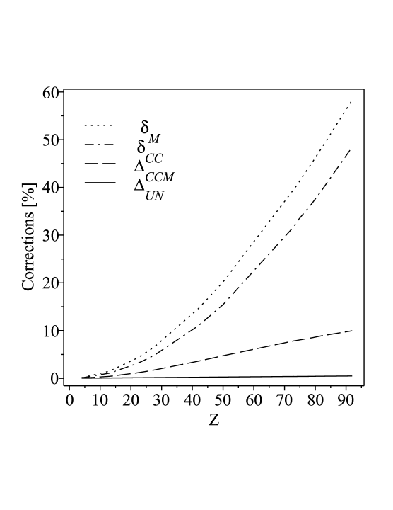
Figure 1: The dependence of the relative Coulomb ($\delta_{\scriptscriptstyle CC}$) and Molière ($\delta_{\scriptscriptstyle M}$) corrections to the screening angle, their difference ($\Delta_{\scriptscriptstyle CCM}$), and the unitarity correction ($\delta_{\scriptscriptstyle UN}$) on the nuclear charge $Z$.

4 Summary

1. Within the framework of fully unitary Glauber approximation for particle-atom scattering, we develop the general formalism of the Molière–Fano multiple scattering theory.

2. We have estimated the relative unitarity correction $\delta_{\scriptscriptstyle UN}\equiv\delta_{\scriptscriptstyle UN}(\sigma)=\delta_{\scriptscriptstyle UN}(W)$ to some quantities of the M–F theory resulting from reconstruction of its unitarity in the second-order optical model of the Glauber theory, and we found that they are of an order of $Z\alpha^{2}$.

3. Within the eikonal approach, we have considered rigorous relations between the exact and Born values of the quantities $\ln\left[g(\eta)\right]$ and $\ln\big{(}\chi_{a}^{\,\prime}\big{)}$. Also, we calculated the Coulomb corrections $\Delta_{\scriptscriptstyle CC}\equiv\Delta_{\scriptscriptstyle CC}\left[\ln\big{(}\chi_{a}^{\,\prime}\big{)}\right]=\Delta_{\scriptscriptstyle CC}\left[\ln g(\chi_{c})\right]$ and relative Coulomb corrections $\delta_{\scriptscriptstyle CC}\equiv\delta_{\scriptscriptstyle CC}\big{(}\chi_{a}^{\,\prime}\big{)}=\delta_{\scriptscriptstyle CC}\left[g(\chi_{c})\right]=\delta_{\scriptscriptstyle CC}\left[W_{\scriptscriptstyle M}(\chi_{c},t)\right]$ for nuclear charge ranged from $Z=4$ to $Z=92$, and we showed that these corrections increase up to $40$ and $50\%$, correspondingly, for $Z=92$.

4. Besides, we have obtained analytical and numerical results for the Coulomb corrections to the parameters of the Molière expansion method ($b^{\scriptscriptstyle B}$, $B^{\scriptscriptstyle B}$, and $\big{(}\overline{\theta^{2}}\big{)}^{\scriptscriptstyle B}$), which depend on the sizes of $B^{\scriptscriptstyle B}$ and Z. We have examined their $B^{\scriptscriptstyle B}$ and $Z$ dependences over the ranges $4.5\leq B^{\scriptscriptstyle B}\leq 20.5$ and $4\leq Z\leq 92$, and found that while the correction $\delta_{\scriptscriptstyle CC}\!\big{(}\overline{\theta^{2}}\big{)}$ becomes the value about 11%, the corrections $-\Delta_{\scriptscriptstyle CC}[B]\times 10^{2}$ and $-\Delta_{\scriptscriptstyle CC}[b]\times 10^{2}$ become very large value (about $40\div 50$) at small $B^{\scriptscriptstyle B}$ and large $Z$.

5. Additionally, we have evaluated the inaccuracies of the Molière theory in determining the relative Coulomb correction to the screening angle. We shoved that its absolute inaccuracy $\Delta_{\scriptscriptstyle CCM}$ reach about $10\%$ for $Z=92$, and the corresponding relative inaccuracy $\delta_{\scriptscriptstyle CCM}$ varies between 30 and 17% over the range $4\leq Z\leq 92$.

Appendix: Derivation of the transport equation for the Bessel-transformed distribution function

We put here the details of inferring Eq. (6). We apply first the integration operation $\int\nolimits_{0}^{\infty}\theta d\theta J_{0}(\eta\theta)$ to both sides of (5). Using the definition of the Bessel transform of the probability distribution (4), we obtain

$$\frac{\partial g(\eta,t)}{\partial t}=-n_{0}\,g(\eta,t)\int\nolimits_{0}^{\infty}\sigma_{el}(\chi)\chi d\chi+n_{0}\int\nolimits_{0}^{\infty}\sigma_{el}(\chi)\chi d\chi I(\eta,\chi)$$ (114)

with

$$I(\eta,\chi)=\int\limits_{0}^{2\pi}\frac{d\phi}{2\pi}\int\theta d\theta J_{0}(\eta\theta)W_{\scriptscriptstyle M}\left(\left|\vec{\chi}-\vec{\theta}\right|,t\right)\ .$$ (115)

Applying the opposite Bessel transform to the probability (5), we get for the last integral

$$I(\eta,\chi)=\int\limits_{0}^{2\pi}\frac{d\phi}{2\pi}\int\theta d\theta J_{0}(\eta\theta)\int\limits_{0}^{\infty}\eta_{1}d\eta_{1}J_{0}\left(\eta_{1}\left|\vec{\chi}-\vec{\theta}\right|\right)g(\eta_{1},t)\ ,$$ (116)

where the integration over $\theta$ can be performed using the folding theorem

$$\int\limits_{0}^{2\pi}\frac{d\phi}{2\pi}J_{0}\left(\eta_{1}\left|\vec{\chi}-\vec{\theta}\right|\right)=J_{0}(\eta_{1}\theta)J_{0}(\eta_{1}\chi)\ .$$ (117)

With the means of the orthogonality relation for the Bessel functions

$$\int\limits_{0}^{\infty}xdxJ_{0}(xa)J_{0}(xb)-\frac{1}{a}\delta(a-b),$$ (118)

we get for $I(\eta,\chi)$:

$$I(\eta,\chi)=g(\eta,t)J_{0}(\eta\chi)\ .$$ (119)

Inserting (119) into (114), we immediately arrive at a result:

$$\frac{\partial g(\eta,t)}{\partial t}=-n_{0}\,g(\eta,t)\int\limits_{0}^{\infty}\sigma_{el}(\chi)\chi d\chi[1-J_{0}(\eta\chi)]\ .$$

To prove the folding theorem (117), we use the series expansion for the Bessel function

$$J_{0}(z)=1-\frac{(z^{2}/4)}{(1!)^{2}}+\frac{(z^{2}/4)^{2}}{(2!)^{2}}-\ldots,$$ (120)

$$z^{2}=\eta^{2}\left[\theta^{2}+\chi^{2}-2\theta\chi\cos\phi\right]$$ (121)

and perform the integration over $\phi$:

$$\frac{1}{2\pi}\int\limits_{0}^{2\pi}(\cos\phi)^{2n}d\phi=\frac{(2n-1)!!}{(2n)!!}\ .$$ (122)

References

- [1] G. Molière, Z. Naturforsch., 2 a (1947) 133.
- [2] G. Molière, Z. Naturforsch., 3 a (1948) 78, 10 a (1955) 177.
- [3] U. Fano, Phys. Rev., 93 (1954) 117.
- [4] DIDAC-Collaboration: B. Adeva, L. Afanasyev, M. Benayoun et al., Phys. Lett., B 704 (2011) 24, B619 (2005) 50; A. Dudarev et al., DIRAC note 2005-02.
- [5] N.O. Elyutin et al., Instrum. Exp. Tech., 50 (2007) 429; J. Surf. Invest., 4 (2010) 908.
- [6] MuScat Collaboration: D. Attwood et al. Nucl. Instrum. Meth., B 251 (2006) 41; A. Tollestrup and J. Monroe, NFMCC technical note MC-176, September 2000.
- [7] R.C. Fernow, MUC-NOTE-COOLTHEORY-336, April 2006; A. Van Ginneken, Nucl. Instr. Meth., B 160 (2000) 460; C.M. Ankebrandt et al. Proposal of the MUCOOL Collaboration, April 2012.
- [8] S.I. Striganov, Radiat. Prot. Dosimetry, 116 (2005) 293.
- [9] A.V. Butkevich, R.P. Kokoulin, G.V. Matushko et al. Nucl. Instrum. Meth. Phys. Res., A 488 (2002) 282.
- [10] V.I. Yurchenko, JETP, 89 (1999) 223.
- [11] F.S. Dzheparov et al., JETP Lett., 72 (2000) 518, 78 (2003) 1011; J. Surf. Invest., 3 (2009) 665.
- [12] A.P. Radlinski, E.Z. Radlinska, M. Agamalian et al., Phys. Rev. Lett., 82 (1999) 3078; H. Takeshita, T. Kanaya, K. Nishida et al., Phys. Rev., E 61 (2000) 2125; M. Hainbuchner, M. Baron, F. Lo Celso et al., Physica (Amsterdam), A 304 (2002) 220.
- [13] H.A. Bethe, Phys. Rev., 89 (1953) 1256.
- [14] H. Snyder and W.T. Scott, Phys. Rev., 76 (1949) 220; W.T. Scott, Phys. Rev., 85 (1952) 245.
- [15] L.A. Kulchitsky and G.D. Latyshev, Phys. Rev., 61 (1942) 254.
- [16] S.A. Goudsmit and J.L. Saunderson, Phys. Rev., 57 (1940) 24, 58 (1940) 36
- [17] R.J. Glauber, in: Lectures in Theoretical Physics, v.1, ed. W. Brittain and L.G. Dunham. Interscience Publ., N.Y., 1959, 315 p.
- [18] A. Tarasov and O. Voskresenskaya, J. Phys., G 40 (2013) 095106.
- [19] I.S. Gradshtein and I.M. Ryzhik, Table of Integrals, Series and Products, Nauka Publication, Moscow, 1971.
- [20] A.V. Tarasov, S.R. Gevorkyan, and O.O. Voskresenskaya, Phys. Atom. Nucl., 61 (1998) 1517.
- [21] Handbook of Mathematical Functions, Eds. M. Abramowitz and I.A. Stegun, National Bureau of Standards, Applied Mathematics Series, 1964.
- [22] E. Kuraev, O. Voskresenskaya, and A. Tarasov, arXiv:1312.7809 [hep-ph], 2013.
- [23] O. Voskresenskaya and A. Tarasov, arXiv:1204.3675 [hep-ph], 2012.
- [24] P.L. Anthony, R. Becker-Szendy, P.E. Bosted et al. Phys. Rev. Lett., 75 (1995) 1949, 76 (1996) 3550; Phys. Rev., D 56 (1997) 1373.