Prospects of coherent control in turbid media: Bounds on focusing broadband laser pulses.

Abstract

We study the prospects of controlling transmission of broadband and bi-chromatic laser pulses through turbid samples. The ability to focus transmitted broadband light is limited via both the scattering properties of the medium, and the technical characteristics of the experimental set-up. There are two time scales, given by pulse stretching in the near- and far-field regions, which define the maximum bandwidth of a pulse amenable to focusing. In the geometric optics regime of wave propagation in the medium, a single set-up can be optimal for focusing light at frequencies ${\omega}$ and $n{\omega}$ simultaneously, providing the basis for the $1+n$ coherent quantum control. Beyond the regime of geometric optics, we discuss a simple solution for the shaping, which provides the figure of merit for one’s ability to focus simultaneously several transmission modes.

I Introduction.

This work is motivated by the goal of applying quantum coherent control techniques in turbid samples. One of the basic ideas of quantum control involves focusing laser fields of the frequencies ${\omega}$ and $n{\omega}$ onto an object with nonlinear response. Interference of the excitation pathways due to each frequency component creates an asymmetric excitation ShapiroBrumerBook . This effect has been demonstrated in a number of theoretical and experimental works devoted to generating directed currents, control of absorbtion and propagation of light, and breakup processes in various physical and chemical systems ShapiroBrumerBook ; CohControl-JPB08 ; Dantus-Review ; Silberberg-Review ; CohControl-1 . Extensions of this principle, based on applying ultrafast laser pulses with controlled broad spectrum, have lead to numerous applications in control of quantum evolution, quantum information processing, spectral characterization, detection, microscopy and manipulations with microscopic and nano-scopic objects ShapiroBrumerBook ; CohControl-JPB08 ; Dantus-Review ; Silberberg-Review ; Rabitz ; RiceBook ; ShapedControl . We are interested in both the ”$1+n$” scenario and control with shaped ultrafast pulses. This task requires an ability to focus either bi-chromatic or broadband laser pulses with shaped spectrum in space in time.

As a laser pulse is applied to a turbid sample – such as ground glass, biological tissue, paint, suspension, plastic, etc – its temporal and spatial structure breaks down Ishimaru-Book ; Tatarski-book ; Goodman-book ; Lagendijk-review ; Genack-review . In space, a coherent beam breaks into a multitude of speckles, so that spatial focusing is destroyed. In the spectral domain, the spectrum at each point in space can be strongly modified, so that the pulse shape is destroyed. The two effects are related, and each of them is deleterious for coherent control.

This paper analyzes control of transmission of light with multiple frequency components in turbid samples, with the goal of designing quantum control experiments. For narrowband light, the corresponding technique Mosk-OptLett07 has recently lead to a breakthrough in focusing and manipulating laser beams in opaque samples Cizmar-NPhot10 ; Gigan-TMeasure-PRL10 ; Mosk-NPhot10 ; Mosk-PRL08 . The method is based on using a two-dimensional phase mask for the spatial correction of the wave front. We analyze the capabilities of this approach for spatio-temporal shaping of ultrafast laser pulses. While the first tests have demonstrated the great potential of the method for temporal focusing Chatel-Focusing-11 ; Lagendijk-Focusing-11 ; Silberberg-11 , efficiency of control over the broad bandwidth of ultrafast pulses needs to be thoroughly understood. Indeed, an experimental set-up optimized for controlling transmission at one given frequency, may not be suitable for another Mosk-BBfocusing-OL11 . A set-up built to focus light at many frequencies simultaneously may be far from optimal for each individual spectral component. This work questions the fundamental limits of controlling broadband transmission through an opaque sample Cizmar-NPhot10 ; Gigan-TMeasure-PRL10 ; Mosk-NPhot10 ; Mosk-PRL08 ; Lagendijk-Focusing-11 ; Silberberg-11 ; Mosk-BBfocusing-OL11 .

We find that the the ability to focus transmitted broadband light is limited via both the scattering properties of the medium, and the characteristics of the Spatial Light Modulator (SLM) used to modify the incident wave front. There are two time scales, given by pulse stretching in the near- and far-field regions (defined further in the text), which set the upper limit of the bandwidth of a pulse that can be focused. Their consideration suggests an optimization of the experimental set-up. In the geometric optics regime of wave propagation inside the sample, a single set-up can be optimal for focusing light at frequencies ${\omega}$ and $n{\omega}$ simultaneously, providing the basis for the $1+n$ coherent quantum control, as demonstrated by our numerical simulations. Beyond geometric optics, i.e. when multiple interference can not be neglected, there is a simple figure of merit for one’s ability to focus simultaneously several transmission modes in space. We also discuss a potential ability of using an opaque sample for shaping broadband spectrum, effectively replacing the dispersion element in the conventional pulse shaper Silberberg-11 ; Lagendijk-Focusing-11 .

The rest of the paper is organized as follows. In the next Section we describe the implied experimental set-up, formulate our task in details, and describe the numerical simulations used throughout the text for illustration purposes. In Section III we neglect dispersion and backscattering, and solve the problem in the geometric optics regime, where the typical scatterer size is bigger than the laser wavelength. Thus we find the bounds on focusing imposed by the finite modulation depth of the SLM. In Section IV, we extend the description, including the effects of dispersion, finite spatial resolution of the phase masks’s pixels, and of focusing of a laser pulse in time and at an angle. We also discuss focusing of broadband pulses in time vs. focusing in space. The general case, which goes beyond the geometric optics regime, is considered in Section V, where we discuss the scaling of the problem, and a simple strategy for using SLM to control simultaneously several independent transmission modes. In the last Section we summarize the findings of this paper.

II Set-up.

Fig.1(a) shows the general set-up according to Refs. Cizmar-NPhot10 ; Gigan-TMeasure-PRL10 ; Mosk-NPhot10 ; Mosk-PRL08 ; Lagendijk-Focusing-11 ; Silberberg-11 . The wavefront of a laser beam is modified by a two-dimensional SLM, whose pixels add a phase to the incident wavefront. The beam is then sent onto the scattering sample. Such a configuration allows the optimization of spatio-temporal focusing in either the near- or far field.

Below, the “near field region”, $E_{near}(x,y,{\omega})$, corresponds to the output surface of this sample. The other, ”far field” region, with the field distribution $\tilde{E}$, is at infinity along the $z$ axis For a spatial harmonic transmitted at an angle $\theta$,

$$\tilde{E}(k,\theta)=\int E_{near}(x,y)\,\exp[ikx\sin\theta]\,dx\,dy$$ (1)

In this paper we concentrate on scattering that is sufficiently treated in the eikonal regime. We limit our consideration to focusing in the far-field, since it allows for easier modelling. This would be equivalent to optimizing transmission into a particular spatial harmonic of $E_{near}$, which can be then focused with a lens. As we explain below, the temporal structure of the pulse remains largely undisturbed in the considered regime and we primarily discuss focusing in space.

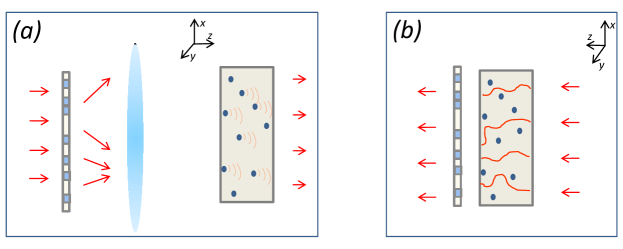
Figure 1: (Color online)Implied experimental set-up. In panel (b), the SLM and imaging lens are replaced by the image of the SLM on the input surface of the sample. In addition, the direction of light propagation is reversed.

Numerically, we solve the scalar wave equation for the electric field amplitude in the parabolic approximation Ishimaru-Book . The random medium is modelled by a set of planes. Each plane modifies the wave front as if the light was passing through a thin glass slide (refractive index $n=1.51$) with randomly placed ”impurities” characterized by a variation ${\Delta}n$ in the refractive index. An example is shown in Fig.2(a). Here the glass slide is taken to be 10-$\mu$m thick, and round Gaussian-shaped impurities of the $1/e$ radius $\sigma=30$-$\mu$m are characterized by ${\Delta}n\leq 0.2$. In the calculations, we place several such planes one after another, separating them by regions of empty space.

Such modelling is inspired by experiments with diffusors based on random arrays of microlenses, ground glass, and all other opaque materials with relatively large (at least several microns in size) impurities Exps-Silberberg ; Cui-11 ; RPCdiffusors . A single slide in our modelling creates a far-field speckle pattern, but does not strongly modify the pulse spectrum. An array of slides, placed one after another, modifies both the spatial and temporal structure of a broadband pulse. Although our modelling misses the effects of de-polarization and backscattering, it allows one to understand some of the most important aspects of random propagation in the regime of low to moderate scattering angles (small backscattering). At the same time, the calculations are fast, allowing us to look at many frequency modes. Numerical propagation at each frequency consists of applying a coordinate-dependent phase to the wavefront at the location of each glass slide, followed by free propagation between the slides. The latter is made by making Fourier transform into the wave vector space and applying a $k$-dependent phase to each spatial mode. For a femtosecond laser pulse sent into the sample, the temporal shape is obtained as a Fourier transform of the transmitted spectrum.

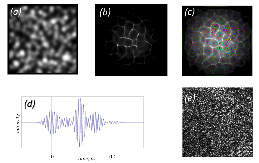
Figure 2: (Color online).(a). Distribution of impurities in one of the four planes modelled in the calculation. The area shown is $770\times 770$ $\mu$m. (b,c) Near-field intensity and phase distributions for a ${\lambda}_{0}=800$ nm beam after passing through four diffusing planes separated by regions of empty space. In panel (c), intensity is shown by brightness, and phase, between 0 and 2$\pi$, is shown by color. (d) A 25-fs input pulse exits the system in the far field stretched to 100 fs. (e) Far-field speckle pattern for 800-nm light.

Fig.2(b) shows the near-field intensity of a 200-$\mu$m-wide beam which has passed through a set of five planes with ${\sigma}=30$ $\mu$m impurities. Adjacent planes are separated by 30 $\mu$m of empty space. In the regime of geometric optics (${\sigma}\gg{\lambda}$), the speckle pattern is mainly due to multiple random lensing. Fig.2(c) shows the same beam, stressing the phase at the exit from the last plane. The phase pattern is shown for the wavelength ${\lambda}=800$ nm. The speckle pattern at each frequency is almost the same, except for a frequency dependent phase which corresponds to a different time delay of the pulse arriving at different $x,y$ points. The zeroth spatial harmonic is $\tilde{E}_{0}=\int E_{near}(x,y)\,dx\,dy$. A 25-fs pulse sent to the system stretches in the far field to about 100 fs, as shown in Fig.2(d). Fig.2(e) shows the far-field speckle pattern for a ${\lambda}=800$ nm beam in the absence of the wave front compensation.

Here we propose to image the SLM onto the input surface of a sample. Hereafter, we refer to the image of the SLM as ISLM. In this geometry, maximizing the transmission from the 0-th to the 0-th spatial mode ($\tau_{00}$) is achieved simultaneously for forward- and for backward- propagating beams. Thus each pixel of the phase mask must add to the backward-propagating beam an $x,y$-dependent phase such as to make the wavefront phase as flat as possible (Fig.1(b)).

Within the arrangement of Fig.1(b), we shall use the term ”near field” for the field in the ISLM plane – even if it is placed at some distance from the actual border of the turbid sample.

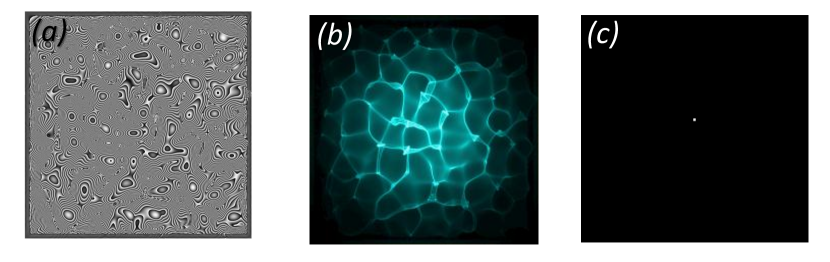
Figure 3: (Color online)(a) Phase mask applied by ISLM to correct the wave front shown in Fig.2(c). (b) Near-field intensity and phase distribution at 800 nm after the phase correction. (c) Corrected far-field intensity distribution.

III The role of the SLM’s parameters.

ISLM can be thought of as a thin transparent plate with variable refractive index $n_{SLM}(x,y)$. A wavefront passing through it acquires the phase

$$\phi_{SLM}(x,y)=k{\alpha}_{0}-k{\alpha}(x,y)$$ (2)

where the optical pathways ${\alpha}_{0}-{\alpha}(x,y)$ are defined by $n_{SLM}(x,y)=n_{0}+{\Delta}n_{SLM}(x,y)$. Fig.3 shows focusing of the ${\lambda}_{0}=800$ nm wave shown in Fig.2, with an ISLM of infinite spatial resolution, and a phase modulation depth of $2\pi$ $(0\leq{\alpha}(x,y\leq\lambda_{0})$. Panel (a) shows the mask ${\alpha}(x,y)$ ranging from 0 (black) to ${\lambda}_{0}$ (white). Panel (b) shows the corrected wavefront. Flat phase of the near-field wavefront ensures that the wave is almost perfectly focused in the far field, as seen in Panel (c). Variations in the near-field intensity somewhat decrease the focusing efficiency, adding a broad low-intensity pedestal, invisible at the scale of Fig. 3(c).

We begin by neglecting dispersion and backscattering, and considering propagation in the eikonal regime. The latter corresponds to impurities in the sample being large, $|\nabla n|\ll k$, where $k$ is the wave vector Tatarski-book . Experiments using commercially available diffusors, ground glass, random arrays of waveguides, etc, may fall under this case. In the eikonal regime, the wave is composed of trajectories - ”rays”. Each ray propagates in accord with the laws of geometric optics, and carries the phase $kS$, where $S$ is the optical path. The surface of equal phase at each point is orthogonal to the ray passing through this point; intensity variations are due to the varying density of the rays.

Assume that the SLM’s image has sufficient spatial resolution, and that the SLM is optimized to focus light with the wave vector $k_{0}=2\pi/{\lambda}_{0}$. What happens with a wave characterized by $k=k_{0}+{\Delta}k$? If the maximum ISLM’s depth ${\alpha}$ was infinite, then the phase flattening would work perfectly at each frequency. Indeed, by imaging the SLM mask on the surface of the sample we can effectively build a flat slab out of the sample and ISLM: for each $k$,

$$k\times[{\alpha}_{0}+S_{0}+{\Delta}S(x,y)-{\alpha}(x,y)]=const$$ (3)

where $S(x,y)=S_{0}+{\Delta}S(x,y)$ is the optical path of a ray passing through the point $(x,y)$ at the ISLM’s plane.

However, in reality the modulation depth ${\alpha}$ can cover only a few wavelengths. Assuming ${\alpha}_{max}={\lambda}_{0}$, we have for the compensated wave front at $k_{0}$

$$k_{0}\times[{\alpha}_{0}+S_{0}+{\Delta}S(x,y)-{\alpha}(x,y)]=2\pi j_{xy}+k_{0}({\alpha}_{0}+S_{0})$$ (4)

where $j_{xy}$ is an integer which can vary from one point $(x,y)$ to another. This is the situation shown in Fig.3. The term $k_{0}S_{0}$ is a constant phase which does not influence focusing. For a different wave vector, we have

$$(k_{0}+{\Delta}k)\times[{\alpha}_{0}+S_{0}+{\Delta}S(x,y)-{\alpha}(x,y)]=(k_{0}+{\Delta}k)({\alpha}_{0}+S_{0})+2\pi j_{xy}+{\Delta}k({\Delta}S(x,y)-{\alpha}(x,y))~{}.$$ (5)

The phase compensation (5) will work for any $k$ if the maximum modulation depth ${\alpha}_{max}>{\Delta}S$ for most pathways. If, on the other hand, ${\Delta}S\gg{\alpha}_{max}$, the compensation will not work as soon as ${\Delta}k({\Delta}S-{\alpha})\simeq{\Delta}k{\Delta}S$ exceeds $\pi$ for many points $(x,y)$. Thus

$${\Delta}k_{max}={\pi\over\langle{\Delta}S\rangle}~{}.$$ (6)

According to the Huygens Fresnel principle,

$$\langle{\Delta}S\rangle=c\,{\tau_{far}}~{},$$ (7)

where ${\tau_{far}}$ shows how much a short pulse sent to the system is stretched in the 0-th spatial mode or, equivalently, in the far-field focus. Another way to see this fact is as follows. Consider two points, A and B, at the exit from the sample, such that $S_{A}=S_{B}+\langle{\Delta}S\rangle$. When CW light of the frequency ${\omega}$ is sent into the system, the phase of the field at the points A and B differs by $\phi_{AB}({\omega})=\langle{\Delta}S\rangle{\omega}/c$. At a different frequency, ${\omega}+{\delta}{\omega}$,

$$\phi_{AB}({\omega}+{\delta}{\omega})=\phi_{AB}({\omega})+{\delta}{\omega}\langle{\Delta}S\rangle/c$$ (8)

According to Eq.(1), the complex values of the field from all near-field points are summed to produce a far-field speckle. One can see from Eq.(8) that the detuning ${\delta}{\omega}=\pi c/\langle{\Delta}S\rangle$ corresponds to the speckle pattern being significantly different from that at the frequency ${\omega}$. At this value of the detuning, constructive interference between the fields coming into the far field region from the points A and B turns into a destructive one, and vice versa. Therefore, the frequency correlation length of the far field speckle pattern is, approximately $2{\Delta}{\omega}_{far}=2\pi c/\langle{\Delta}S\rangle$. This means that the transmitted spectrum in the far field consists of independent bands of the width $2{\Delta}{\omega}_{far}$. Equivalently, a very short laser pulse sent into the system stretches in the far field to ${\tau}_{far}=\pi/{\Delta}{\omega}_{far}$.

Comparing Equations (6) and (7), we see that compensation can only work for detunings ${\Delta}{\omega}={\omega}-{\omega}_{0}$ such that

$$|{\Delta}{\omega}|<\frac{\pi}{{\tau_{far}}}\equiv{\Delta}{\omega}_{far}~{}.$$ (9)

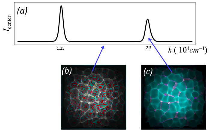
Figure 4: (Color online) (a) Laser intensity in the zeroth far-field mode in dependance on frequency, with the ISLM mask tuned for ${\omega}_{0}$. (b,c) Near-field wave fronts at ${\omega}=1.5{\omega}_{0}$ and ${\omega}=2{\omega}_{0}$.

Figure 4 assumes the compensation mask shown in Fig.3(a) applied to the sample discussed in Figs.2 and 3. Panel (a) shows the intensity $I_{center}$ in the far-field focus in dependance on the field wave vector, calculated for a single realization of the random sample. As $k$ is detuned from $k_{0}=12500$ cm^-1, the focusing vanishes. The width $2{\Delta}k\simeq 500$ cm^-1corresponds, up to a numerical factor of $\simeq 1.5$, to ${\tau_{far}}=100$ fs, i.e. the pulse stretching seen in Fig.2(d).

Unexpectedly, $I_{center}$ in Fig.4 increases again in the vicinity of $k=2\,k_{0}$. The effect is explained in the following way. If the condition (4) is fulfilled, then

$$2k_{0}\times[{\alpha}_{0}+S_{0}+{\Delta}S(x,y)-{\alpha}(x,y)]=4\pi j_{xy}+2k_{0}(S_{0}+S_{0,SLM})~{},$$ (10)

and the phase compensation at twice the main wave number is again complete, as shown in Fig.4(c). We see that in the simplified model — negligible dispersion, ISLM can spatially resolve the phase front, — an ability to focus bi-chromatic fields, and to perform ”1+$n$” quantum control comes at no expense. An experimental set-up optimized to focus a laser field at frequency ${\omega}$ will also focus field at frequency $n{\omega}$.

Note that the peak amplitude at $2k_{0}$ in Fig.4 is slightly smaller than that at $k_{0}$. Indeed, the assumption that the phase mask is able to resolve individual pathways becomes invalid at the near-field caustics, where several rays intersect at the same point. This situation is mathematically similar to that of an SLM with limited spatial resolution, discussed in the next Section.

Moreover, similar to the case of $k=2k_{0}$, at $k=1.5\,k_{0}$ the phase of the compensated wave can only have two values, 0 and $\pi$, as seen in Fig.4(b). Each part of the near-field wave front – that with the zero phase, and the phase equal to $\pi$ – yields a strong focus in far-field. The two foci interfere destructively. However, because of the random amplitudes, the destructive interference is not complete, and focusing at $k=1.5\,k_{0}$ is still better than that at the adjacent values of $k$. Reminiscent of fractional quantum wave packet revivals revivals , such incomplete focusing happens at any $k=P/Q\times k_{0}$ with integer $P,Q$.

IV Additional bounds.

The above consideration remains valid if the goal is to optimize transmission into a spatial harmonic propagating at an angle ${\theta}$ (or, equivalently, off-axis far field focusing). In this case, Eq.(4) turns into

$$k_{0}\times[{\alpha}_{0}+S_{0}+{\Delta}S(x,y)-{\alpha}(x,y)]=2\pi j_{xy}+k_{0}({\alpha}_{0}+S_{0})+k_{0}x\,\sin{\theta}$$ (11)

where $x$ is the coordinate in the ISLM plane. In a compete analogy with Eq.(10), light with the wave vector $2k_{0}$ will also be focused. In our numerical simulations, the spectral bandwidth ${\Delta}k$ of the spatially focused light did not depend on ${\theta}$.

The ability of the scheme to focus several frequencies simultaneously depends on the sample’s dispersion. Indeed, the above consideration is based on the assumption that light at each frequency propagates along the same set of rays. In another series of calculations we included the effect of dispersion, assuming that the samples are made of BK-7 glass BK7 . We found that the focusing survives in the presence of dispersion: In our calculations, the focused intensity at the frequency $2{\omega}_{0}$ decreases only by a factor of, approximately, 2-3. This number is small compared to the $\sim 10^{5}$-fold increase in the intensity at the focus observed in the case of complete phase compensation.

Finite size of the ISLM’s pixels in the $(x,y)$ plane does bring an important additional bound on one’s ability to focus broadband light. If the ISLM grid can not resolve the phase variations in the incident wave front, then each pixel will be used to compensate the phase of the average field

$$E_{av}(k_{0})=\sum_{S}P({\Delta}S_{p})e^{ik_{0}(S_{0}+{\Delta}S_{p})}$$ (12)

where $P({\Delta}S_{p})$ is the probability distribution for the pathways characterized by the length $S_{0}+{\Delta}S_{p}$ averaged by a single pixel. Coarse graining over ISLM’s pixel size limits the compensation fidelity. Suppose that a pixel is tuned to compensate the phase of $E_{av}$ at the given position at the frequency $k_{0}c$. At a different frequency we have

$$E_{av}(k)=\sum_{S}P({\Delta}S_{p})e^{i[kS_{0}+k_{0}{\Delta}S_{p}+{\Delta}k{\Delta}S_{p}]}~{}.$$ (13)

The values of $E_{av}$ correspondent to $k$ and $k+{\Delta}k$ differ drastically if ${\Delta}k{\Delta}S_{p}\sim\pi$ for many pathways passing through the particular pixel. Thus the phase compensation will not work for detunings ${\Delta}{\omega}$ exceeding

$${\Delta}{\omega}_{near}=\frac{\pi}{{\tau_{near}}}$$ (14)

where ${\tau}_{near}=c\,\langle{\Delta}S_{p}\rangle$ describes stretching of the pulse in the near field, averaged over an area of the ISLM’s pixel.

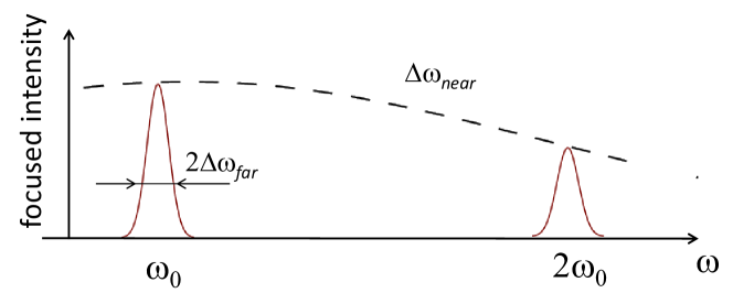
Figure 5: (Color online) Focusing as a function of frequency in the limit of low spatial dispersion.

The bounds on the focusing imposed by the SLM are summarized in Fig.5. There can be several peaks of the focused field, each of the width $2{\Delta}{\omega}_{far}$, under the envelope of the width ${\Delta}{\omega}_{near}$.

Note that ${\Delta}{\omega}_{near}$ is due to the pulse stretching at the ISLM’s pixel. If one moves the ISLM plane away from the surface of the sample, then ${\Delta}{\omega}_{near}$ approaches ${\Delta}{\omega}_{far}$. Same happens if the pixel size is increased, or if interference of multiple pathways at each point of the ISLM plane becomes too strong. We numerically verified that the peak at $2{\omega}_{0}$ in Fig.5 disappears if the ISLM pixels become so large that they can not resolve the phase variations in the scattered wave.

The peak also disappears if the interference in the scattering process can not be neglected. In our calculations, this was achieved by reducing the typical size of the impurities while simultaneously increasing their number. This led to both higher scattering angles, and deviations from the eikonal regime which allows interpreting propagation of light via an ensemble of rays. Surprisingly, however, predictions based on the eikonal optics approach hold even for rather strong scattering: For light that has passed through 30 3-$\mu$m thick planes with ${\sigma}=2$ $\mu$m impurities, the phase compensation for the ${\lambda}_{0}=800$ nm far-field focusing still provided a noticeable focal spot at ${\lambda}={\lambda}_{0}/2=400$ nm.

Our consideration above refers to focusing laser pulses in space, but not in time. Note, however that the ability to spatially focus broadband light is bound by ${\Delta}{\omega}_{far}$ - the spectral bandwidth of a pulse which is not strongly distorted in the far field. Thus we show that the above approach is limited to a spectral band where the temporal structure is not destroyed, and temporal focusing is not required. If the far-field stretching is substantial, one needs to assign different pixels to different bands, as described in the next Section. Only at that stage the question of temporal shaping and focusing – adjusting the relative phases of several independent frequency bands – arises.

V The general case

In the general situation, many interfering pathways may lead to the same near-field point. As before, let ${\tau_{near}}$ characterize the stretching of the pulse at the exit from the sample, and ${\tau_{far}}$ – at infinity. Similar to the previous Section, the near-field speckle pattern changes at detunings exceeding ${\Delta}{\omega}_{n}=\pi/{\tau_{near}}$, and finite depth of the SLM’s phase modulation prevents focusing at detunings exceeding ${\Delta}{\omega}_{f}=\pi/{\tau_{far}}$ except for the frequencies ${\omega}_{m}$ related to ${\omega}_{0}$ by

$$\int k_{m}\,dS(k_{m})=m\times\int k_{0}\,dS(k_{0})~{}.$$ (15)

As shown in Section IV, if ${\tau_{near}}<{\tau_{far}}$, it makes sense to place the ISLM in the near field with respect to the random sample. Note that such situations include those where the pulse is significantly modified after passing through the random sample, both in space and in time.

In the case of stronger scattering, when the geometric optics -based model is inapplicable, one must view the far-field focusing as phasing together random phasors corresponding to different scattering channels Mosk-OptLett07 . This regime is mathematically similar to that of large ISLM pixels, discussed in the previous Section (Eqs.(12-14)). Below we briefly discuss what scaling should be expected for focusing broadband pulses in this case.

Let us assume that the far-field transmission spectrum within the bandwidth of the laser pulse consists of $M$ un-correlated bands of the width ${\Delta}{\omega}_{f}$, and that the laser beam covers $N$ pixels of the phase mask in the scheme of Fig.1(a). In order to obtain figures of merit for the focusing capability, we assign $N/M$ pixels of the SLM to each frequency band, in the way that is discussed below. Assuming a circular gaussian distribution for the field amplitude after the sample Mosk-OptLett07 ; Goodman-book ,

$$P(E_{Re},E_{Im})=\frac{1}{2\pi I_{0}}\exp\left[-\frac{E_{Re}^{2}+E_{Im}^{2}}{I_{0}}\right]$$ (16)

where $P$ is the probability density, and $E_{Re},E_{Im}$ are the real and imaginary field amplitudes, the intensity of the focused field at frequency ${\omega}$ is Goodman-book

$$I_{coh}({\omega})=\frac{\pi}{4}\left(\frac{N}{M}\right)^{2}\,I_{0}~{}.$$ (17)

In order for the focused spectrum to be controllable, this value must exceed the background due to the other pixels assigned to all other frequencies. The latter is obtained with the help of Eq.(16) as

$$\langle I_{back}({\omega})\rangle=(M-1)\frac{N}{M}\,I_{0}~{}.$$ (18)

Enhancement in spectral intensity due to the focusing is then Mosk-OptLett07

$$\eta_{\omega}=\frac{\pi}{4}\frac{N}{M^{2}}~{}.$$ (19)

Once control over each spectral band of the width ${\Delta}{\omega}_{far}$ is achieved, one can tune the overall phase of the field in each band by applying an extra phase to each phase mask’s pixels controlling the mode. Through these phases, the spatially focused pulse can either be focused in time or be given any temporal shape allowed by the frequency resolution of ${\Delta}{\omega}$ and the number of pixels in the phase mask. Thus the system makes an analog of a conventional pulse shaper Wiener , with the dispersion element being replaced by the random sample Silberberg-11 ; Lagendijk-Focusing-11 .

If the $M$ spectral components are given equal phase, together they form a pulse that is $M$ times shorter in time than each of the $M$ components. Its intensity is $M$ times higher than that of the incoherent sum of the components. Thus the maximum achievable intensity is

$$\eta_{t}=\frac{\pi}{4}\frac{N}{M}$$ (20)

times stronger than that of un-compensated light.

VI Summary

Coherent control of physical and chemical processes in turbid media requires availability of focused laser pulses with tunable temporal/spectral shapes. This, in turn, sets the task of coherently controlling propagation of bi-chromatic and broadband laser pulses through turbid media.

Recent works have shown that this task can be carried out by using phase masks to adjust the phases of different transmission modes. Each mode, centered at its own central frequency and having its own speckle pattern, can coherently contribute to the output field. By controlling the interference between the modes one can achieve the desired spatio-temporal focusing. In this sense, the experimental scheme shown in Fig. 1 is an analog of a conventional pulse shaper, with the dispersive element replaced by the turbid sample. Resolution of this turbid pulse shaper is set by the transmission properties of the sample Silberberg-11 , together with one’s technical ability to control relative phases of the modes. The ability to shape pulses simultaneously in space and time, and to work with very narrow-band transmission modes, can bring new dimensions into experiments on coherent control.

Most present-day experiments do not assume correlations between the phase patterns of different frequency bands, and work in the regime where the phase mask can not resolve phase variations within a single speckle pattern. In this case one can obtain the figure of merit for the efficiency of the spatio-temporal focusing of light by assigning a fraction of the phase mask to each of the independent frequency bands. This is done in Section V of our paper (Eqs.(19,20)). For $M$ independent frequency bands, this leads to focused intensity at a single frequency scaling as $\eta_{\omega}\propto 1/M^{2}$. If the phases of the frequency bands are set such as to produce a short pulse in the focus, its intensity scales as $\eta_{t}\propto 1/M$.

An interesting regime arises in the case of moderately strong scattering and relatively large-size (above 2 $\mu$m in our simulations with 800-nm light) scatterers. In this case, in agreement with the geometric optics approach, optimization of spatial focusing at frequency ${\omega}_{0}$ automatically ensures that focusing at the frequency ${\omega}=n{\omega}_{0}$ is also achieved. In this situation, ”1+n” coherent control must be available at no extra cost provided the relative phase between the two fields can be maintained. In addition, interesting phase structures arising at frequencies that are rational fractions of ${\omega}_{0}$ call for further investigation.

In the geometric optics regime, the efficiency of the spatial focusing is bound by the two time scales. A single set-up of the phase mask can only optimize spatial focusing within a single frequency transmission band, with the width given by $2{\Delta}{\omega}_{far}=2\pi/{\tau_{far}}$ (Eq.9), where ${\tau_{far}}$ corresponds to the stretching of an ultrashort pulse in the far field at the output. At the same time, there is an overall envelope of the focusing efficiency (Fig.5). Its width is given by ${\Delta}{\omega}_{near}=\pi/{\tau_{near}}$. Here ${\tau_{near}}$ is the duration of a pulse covered by the area of a single pixel of the phase mask in the geometry of Fig. 1(b), and ${\Delta}{\omega}_{near}$ is the band with of the transmission matrix taken at one pixel. The separation of the two time scales suggests that one should choose the experimental set-up with the shortest ${\tau_{near}}$. To minimize the pulse stretching in the plane of the phase mask, we proposed to image the SLM onto the input surface of the turbid sample.

The intuition inspired by geometric optics remains valid if one considers far-field focusing at an angle, or if moderate dispersion of the sample is taken into account. However, using the same phase mask to focus at frequencies ${\omega}$ and $n{\omega}$ simultaneously becomes difficult if the pixels of the phase mask can not resolve individual near-field speckles. In this case ${\Delta}{\omega}_{near}$ approaches ${\Delta}{\omega}_{far}$, and pulse stretching in the near- and far field is the same. Then the geometry can not be optimized by placing the phase mask at any particular distance from the sample. Control over focusing of multiple frequencies can be achieved by assigning subsets of the mask to different frequency bands.

References

- (1) M. Shapiro and P. Brumer, Principles of the Quantum Control of Molecular Processes (Wiley-Interscience, Hoboken, N.J., 2003).
- (2) M Shapiro , T Baumert and H Fielding, eds, Special Issue on Coherent Control, J. Phys. B 41, no.7 (2008)
- (3) M. Dantus and V. V. Lozovoy, Experimental Coherent Laser Control of Physicochemical Processes, Chem. Rev. 104, 1813 (2004), and references therein.
- (4) Y. Silberberg, Annu. Rev. Phys. Chem. 60 (2009) and references therein.
- (5) See e.g. D. Sun, C. Divin, J. Rioux, J.E. Sipe, et al., Nano Lett. 10, 1293 (2010); Dupont, E.; Corkum, P. B.; Liu, H. C.; Buchanan, M.; Wasilewski, Z. R., Phys. Rev. Lett. 74, 3596 (1995); D. Meshulach and Y. Silberberg, Nature 396, 239 (1998); V. Blanchet, C. Nicole, M. A. Bouchene, B. Girard, Phys. Rev. Lett. 78, 2716 (1997).
- (6) W.S. Warren, H. Rabitz, and M. Dahleh, Science 259, 1581 (1993).
- (7) S.A. Rice and M. Zhao, Optical Control of Molecular Dynamics (Wiley-Interscience, Hoboken, N.J., 2000).
- (8) See e.g. J. Ahn, T. C. Weinacht, and P. H. Bucksbaum, Science 287, 463 (2000); Z. Amitay, R. Kosloff, and S. R. Leone, Chem. Phys. Lett. 359, 8 (2002); A. Assion, T. Baumert, M. Bergt, T. Brixner, B. Kiefer, V. Seyfried, M. Strehle, and G. Gerber, Science 282, 919 (1998); E.A. Shapiro, I.A. Walmsley, M.Yu. Ivanov, Phys. Rev. Lett. 98, 050501 (2007); R. J. Levis, M. Menkir, and H. Rabitz, Science, 292, 709 (2001); R. Bartels, S. Backus, E. Zeek, et. al., Nature, 406, 164, (2000); X. Li, G.A. Parker, J. Chem. Phys. 128, 184113 (2008); C.P. Koch, R. Kosloff, Phys. Rev. Lett. 103, 260401 (2009); P. Kral, I. Thanopulos, and M. Shapiro, Rev. Mod. Phys. 79, 53 (2007).
- (9) A. Ishimaru, Wave propagation in random media (Academic Press, New York, 1978).
- (10) V.I. Tatarski, Wave propagation in turbulent atmosphere (Rus.) (Nauka, Moscow, 1967).
- (11) J.W. Goodman, Statistical optics (John Wiley and Sons, New York, 2000), chapter 2.
- (12) A.Z. Genack, Fluctuations, Correlation and Average Transport of Electromagnetic Radiation in Random Media, in Scattering and localization of classical waves in random media, P. Sheng, ed. (World Scientific, Singapore, 1990).
- (13) A. Lagendijk, B.A. van Tiggelen, Phys. Rep. 270, 143 (1996).
- (14) I. M. Vellekoop and A. P. Mosk, Opt. Lett. 32, 2309 (2007).
- (15) S.M. Popoff, G. Lerosey, R. Carminati, M. Fink, A. C. Boccara, S. Gigan, Phys. Rev. Lett. 104, 100601 (2010).
- (16) I. M. Vellekoop and A. P. Mosk, Phys. Rev. Lett. 101, 120601 (2008).
- (17) I.M. Vellekoop, A. Lagendijk, A.P. Mosk, Nature Photonics 4, 320 (2010).
- (18) T. Cizmar, M. Mazilu and K. Dholakia, Nature Photonics 4, 388 (2010).
- (19) O. Katz, Y. Bromberg, E. Small, Y. Silberberg, Nature Photonics 5,372 (2011).
- (20) D.J. McCabe, A. Tajalli, D.R. Austin, P. Bondareff, I.A. Walmsley, S. Gigan, and B. Chatel, Nature Communications 2 447 (2011).
- (21) J. Aulbach, B. Gjonaj, P.M. Johnson, A.P. Mosk, A. Lagendijk, Phys. Rev. Lett. 106, 103901 (2011).
- (22) F. van Beijnum, E. G. van Putten, A. Lagendijk, and A. P. Mosk, Opt. Lett. 36, 373 (2011)
- (23) E. Tal, Y. Silberberg, Opt. Lett. 31, 3529 (2006).
- (24) M. Cui, Opt. Lett. 36, 870 (2011); M. Cui, Opt. Express 19, 2989 (2011).
- (25) See the bibliography on the use of Engineered diffusors at the web site of RPC Photonics, http://www.rpcphotonics.com/literature.asp (accessed on July 22, 2011).
- (26) I. S. Averbukh, N. F. Perelman, Phys. Lett. A 139, 449 (1989); E.A. Shapiro, Sov. Phys. JETP 91(3), 449 (2000).
- (27) Refractive index database, http://refractiveindex.info , as accessed on 06.06.2011.
- (28) A. M. Weiner, Rev. Sci. Instrum. 71, 1929 (2000).