Higgs Phenomenology in Warped Extra-Dimensions with a 4th Generation

Abstract

We study a warped extra-dimension scenario where the Standard Model fields lie in the bulk, with the addition of a fourth family of fermions. We concentrate on the flavor structure of the Higgs couplings with fermions in the flavor anarchy ansatz. Even without a fourth family, these couplings will be generically misaligned with respect to the SM fermion mass matrices. The presence of the fourth family typically enhances the misalignment effects and we show that one should expect them to be highly non-symmetrical in the ${(34)}$ inter-generational mixing. The radiative corrections from the new fermions and their flavor violating couplings to the Higgs affect negligibly known experimental precision measurements such as the oblique parameters and $Z\to b{\bar{b}}$ or $Z\to\mu^{+}\mu^{-}$. On the other hand, $\Delta F=1,2$ processes, mediated by tree-level Higgs exchange, as well as radiative corrections to $b\to s\gamma$ and $\mu\to e\gamma$ put some generic pressure on the allowed size of the flavor violating couplings. But more importantly, these couplings will alter the Higgs decay patterns as well as those of the new fermions, and produce very interesting new signals associated to Higgs phenomenology in high energy colliders. These might become very important indirect signals for these type of models as they would be present even when the KK mass scale is high and no heavy KK particle is discovered.

I Introduction

The Standard Model (SM) of particle physics has been remarkably successful in explaining a wide range of low-energy phenomena and has passed numerous experimental tests over the past few decades. The only ingredient of this model that has yet to be discovered is the Higgs boson. If the Higgs is discovered at the LHC, the problem of its mass, which should receive quadratic corrections sensitive to scales well above the electroweak scale (the hierarchy problem) still remains. Warped extra dimensional models were introduced by Randall and Sundrum (RS) RS as an attempt to resolve this problem, by using the extra-dimensional space-time warp factor to lower the natural scale of particle masses. In the original model, all SM fields were localized on the TeV brane, one could in principle generate higher dimensional flavor violating operators, suppressed by only TeV operators–a serious problem for phenomenology. To address this issue one could invoke for example flavor symmetries Sundrum:2009gv but the most popular venue has been to allow fermions to propagate in the bulk, which not only reduced the flavor problem, but provided a compelling theory of flavor, in which hierarchies among fermion masses and mixings arise naturally Davoudiasl ; Grossman:1999ra . This model sheds light on the flavor puzzle as well: the 5D Yukawa couplings are all ${\cal O}(1)$ and with no definite flavor structure, and the fermion masses and mixing angles depend on the amount of mixing of the elementary fermions with the strongly coupled conformal field theory, assumed to be small for the first two generations Grossman:1999ra . This implies that flavor violation in the SM is also suppressed by the same mixing factors - the phenomenon that goes under the name of the RS-GIM mechanism agashe . However, in this case constraints from the $\Delta S=2$ and $\Delta B=1$ processes still require the scale of new physics (the KK scale) to be around $\sim 5$ TeV Agashe2site ; Gedalia:2009ws , raising difficulties with observation of this minimal scenario directly at the LHC.

On the flavor side, recently, some possible deviations from the SM in $B$ meson Bphysics ; Abazov:2011yk and $t$ quark physics newcdf have been reported, indicating perhaps difficulties with the standard Cabibbo-Kobayashi-Maskawa (CKM) paradigm for quark mixing Lunghi:2010gv . The effects in $B$ physics can be explained by various Beyond the Standard Model (BSM) scenarios, though the simplest explanation seems to come from a simple extension of the Standard Model to four generations, that is, by adding two new heavy quarks, a heavy charge $+2/3$ quark ($t^{\prime}$) and charge $-1/3$ quark ($b^{\prime}$). In more extensive versions of the model, the effects of introducing extra leptons ($\tau^{\prime}$ and $\nu_{\tau}^{\prime}$), needed for anomaly cancellation, are also studied.

The addition of a fourth sequential generation of fermion doublets is a natural extension of the SM (SM4). The model restricts fourth-generation quark masses to be not too large to preserve perturbativity marciano . Recently, SM4 have increased in popularity as it was shown that the introduction of a fourth generation does not conflict with electroweak precision observables holdom , as long as their mass differences are small yanir . Fourth generation fermions are required to have masses greater than half the mass of the $Z^{0}$ boson to evade LEP limits on the invisible $Z^{0}$ boson width. There are many advantages of introducing an extra family of fermions:

• These new fermions may trigger dynamical electroweak symmetry breaking marciano without a Higgs boson, and thus address the hierarchy problem.

• A fourth generation softens the current low Higgs mass bounds from electroweak precision observables by allowing considerably higher values for the Higgs mass flacher .

• Gauge couplings can in principle be unified without invoking SUSY hung .

• A new family might cure certain problems in flavor physics, such as the CP-violation in $B_{s}$-mixing soni .

• A fourth generation might solve problems related to baryogenesis, as an additional quark doublet could lead to a sizable increase of the measure of CP-violation hou .

• Such an extension of the SM would increase the strength of the phase transition carena .

• It appears that an even number of fermion generations is more natural from the string theory point of view Cvetic:2001nr .

New heavy fermions lead to new interesting effects due to their large Yukawa couplings hung2 . Recent searches by the CDF Collaboration for direct production of the fourth generation quarks, called $t^{\prime}$ and $b^{\prime}$, set the limits $m_{t^{\prime}}>335$ GeV CDF and $m_{b^{\prime}}>385$ GeV CDF2 , assuming Br$\left(t^{\prime}\to Wq(q=d,s,b)\right)=100\%$ and Br$(b^{\prime}\to Wt)=100\%$ respectively. For the leptons $m_{\tau^{\prime}}>100.8$ GeV, $m_{\nu_{\tau}^{\prime}}>90.3$ GeV  (Dirac type), $m_{\nu_{\tau}^{\prime}}>80.5$ GeV (Majorana type) particledata . The limits on the low energy phenomenology due to fourth generation fermions has been studied extensively UTfit ; Alok:2010zj .

While there have been many extensive studies of the SM4, there are few analyzes of BSM scenarios with four generations (see however DePree:2009ed ). The reason is that the fourth generation typically imposes severe restrictions on the models. In particular, there are difficulties in incorporating a chiral fourth family scenario into any Higgs doublet model, such as the MSSM Murdock:2008rx . It was initially shown that due to the large masses for the fourth generation quarks and large Yukawa couplings, there are no values of $\displaystyle\tan\beta=\frac{v_{u}}{v_{d}}>1$ for which the couplings are perturbative to the Grand Unification Scale. (However, this condition does not apply to vector-like quarks Atre:2011ae .) Recently the MSSM with four generations has received some more attention Cotta:2011ht , as it was shown that for $\tan\beta\simeq 1$ the model exhibits a strong first order phase transition Fok:2008yg .

But the four generation scenario can easily be incorporated in models with warped extra dimensions, as in Burdman:2009ih , where it can be argued that the fourth generation arises naturally. In these models the Higgs particle can be thought of as a generic composite state, and even being a condensate of some of the fourth generation heavy quarks Burdman:2009ih ; BarShalom:2010bh , thus providing a solution to the (little) hierarchy problem.

An additional benefit of the extension of a fourth generation in warped models, could be the inclusion of the fourth generation neutrino, which may become a novel dark matter candidate Lee:2011jk , typically missing in minimal models (see however Agashe:2009ja for different approaches).

As mentioned earlier, KK particles could be just barely beyond the reach of the LHC. Nevertheless there are implications of the warped scenarios that could leave an imprint on lower energy physics. For instance, recently it was pointed out that warped extra-dimensional models introduce new flavor-violating operators in the Higgs sector. In a composite Higgs sector with strong dynamics, flavor changing neutral currents (FCNC) can arise at tree level, generated by a misalignment between the Higgs Yukawa matrices and the fermion mass matrices Buchmuller:1985jz ; Agashe:2009di ; toharia1 . The full set of operators responsible for the misalignment has been thoroughly analyzed, showing that the effect is generically large and phenomenologically important toharia1 and even could alter considerably the couplings of Higgs to gluons Casagrande:2010si ; toharia2 , affecting thus the main production mechanism of the Higgs at hadron colliders.

These flavor violating effects will be even more pronounced if the matter sector is extended by extra fermionic generations. And for the Higgs bosons, it is well known that the effects of a fourth generation are quite spectacular in modifying the Higgs boson cross-section at hadron colliders, which can be tested easily with Tevatron and early LHC data within this or the next year. The Tevatron has published limits on the Higgs boson cross-section in the fourth generation model, excluding a wide range of Higgs boson masses HCDF , and recently the CMS collaboration carried out a similar study Chatrchyan:2011tz .

As Higgs production can be modified within warped scenarios due to flavor violating effects in the Higgs sector toharia2 , it may be possible to distinguish signals coming from a fourth generation model within the SM (SM4) with those coming from a fourth generation model associated with a warped extra-dimension (or a composite scenario), and, given the searches for the Higgs boson underway at the LHC, such an analysis is timely. The inclusion of the fourth generation will also affect low-energy precision observables, as well as limits on rare decays. In the lines of toharia1 , we propose to explore here the effect of FCNC Higgs couplings with a fourth generation in a simple warped extra dimensional model.

Our work is organized as follows. In the next section, Sec. II, we summarize the features of the warped extra-dimensional models with fermions propagating in the bulk. We analyze the flavor structure with fourth generational mixing in Sec. III, giving both analytical expressions and numerical values. We proceed to explore the phenomenology of the model in Sec. IV. Restrictions due to flavor-changing low energy observables, both at tree and one-loop level, are included here. In subsections, we investigate FCNC decays of the Higgs boson, as well as collider signals for the fourth generation decaying into lighter fermions and Higgs bosons. We summarize our findings and conclude in Sec. V. In the Appendices we include some details of our analytical evaluation.

II The model

For simplicity, we consider the simplest 5D warped extension of the SM, in which we keep the SM local gauge groups and just extend the space-time by one warped extra dimension. There are bounds on the KK scale coming from precision electroweak observables Agashe:2007mc which can be addressed by extending the gauge group in order to obtain additional protection. Nevertheless the effects we are interested in lie in a different sector of the scenario, namely the Higgs sector, and its couplings with fermions. Our results can easily be extended to more involved scenarios, but we feel it is best to show explicitly the effects in the simplest scenario. Moreover precision electroweak constraints can become milder with a heavier Higgs Casagrande:2008hr and perhaps even if the KK scale is barely beyond LHC reach, one can observe its indirect effects in the Higgs sector.

The spacetime we consider takes the usual Randall-Sundrum form RS :

$$ds^{2}=\frac{R^{2}}{z^{2}}\!\Big{(}\eta_{\mu\nu}dx^{\mu}dx^{\nu}-dz^{2}\Big{)},$$ (1)

with the UV (IR) branes localized at $z=R$ ($z=R^{\prime}$). We first focus on a single family of down-type quarks $Q$, $D$. They contain the 4D SM $SU(2)_{L}$ doublet and singlet fermions respectively with a 5D action

$$S_{\text{fermion}}\!=\!\int d^{4}xdz\sqrt{g}\Big{[}{i\over 2}\left(\bar{Q}\Gamma^{A}{\cal D}_{A}Q-{\cal D}_{A}\bar{Q}\Gamma^{A}Q\right)+{c_{q}\over R}\bar{Q}{Q}+(Q\rightarrow D),$$ (2)

where $c_{q}$ and $c_{d}$ are the 5D fermion mass coefficients. We also consider a brane localized Higgs, and so the Yukawa couplings in the Lagrangian are included in the action

$$S_{\text{brane}}=\int d^{4}xdz\,\delta(z-R^{\prime})\left(\frac{R}{z}\right)^{4}H\left({Y^{5D}_{1}}R\bar{{\cal Q}}_{L}{\cal D}_{R}+{Y^{5D}_{2}}R\bar{{\cal Q}}_{R}{\cal D}_{L}+\text{h.c.}\right).$$ (3)

To obtain a chiral spectrum, we choose the following boundary conditions for $Q,D$

$$Q_{L}(++),\quad Q_{R}(--),\quad D_{L}(--),\quad D_{R}(++).$$ (4)

Then, only $Q_{L}$ and $D_{R}$ will have zero modes, with wavefunctions:

$$q_{L}^{0}(z) = f(c_{q})\frac{{R^{\prime}}^{-\frac{1}{2}+c_{q}}}{R^{2}}z^{2-c_{q}},$$ (5)

$$d_{R}^{0}(z) = f(-c_{d})\frac{{R^{\prime}}^{-\frac{1}{2}-c_{d}}}{R^{2}}z^{2+c_{d}},$$ (6)

where we have defined $f(c)\equiv\sqrt{\frac{1-2c}{1-\epsilon^{1-2c}}}$ and the hierarchically small parameter $\epsilon=R/R^{\prime}\approx 10^{-15}$, which is generally referred to as the warp factor. Thus, if we choose $c_{q}(-c_{d})>1/2$, then the zero modes wavefunctions are localized towards the UV brane; if $c_{q}(-c_{d})<1/2$, they are localized towards the IR brane. The wavefunctions of the fermion KK modes are all localized near the IR brane. Note that the wavefunctions of the KK modes $Q_{R}$ and $D_{L}$ vanish at the IR brane due to their boundary conditions. The Yukawa couplings of the Higgs with fermions (zero modes or heavy KK modes) are set by the overlap integrals of the corresponding wavefunctions. For a bulk Higgs localized near the IR brane, the zero-zero-Higgs, zero-KK-Higgs, KK-KK-Higgs Yukawa couplings are given approximately by

$$Y_{d,00} \sim Y_{*}f(c_{q})f(-c_{d}),$$ (7)

$$Y_{d,0n} \sim Y_{*}f(c_{q})\,\ \text{or}\ \,Y_{*}f(-c_{d}),$$ (8)

$$Y_{d,nm} \sim Y_{*},$$ (9)

where $Y_{*}=Y_{d}/\sqrt{R}$ is the ${\cal O}(1)$ dimensionless 5D Yukawa coupling, and we ignored ${\cal O}(1)$ factors in the equations above. The SM fermions are mostly zero mode fermions with some small amount of mixing with KK mode fermions. Therefore, we can use the mass insertion approximation to calculate the corrections to the masses and Yukawa couplings of SM fermions.

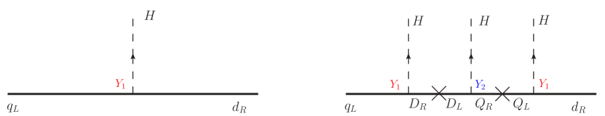
Figure 1: Correction to fermion mass and to physical Yukawa coupling (right diagram) after integrating out heavy vector-like fermions (the fermion KK modes here). In the right diagram, the correction to the mass happens when all the Higgs bosons acquire their VEV. The correction to the Yukawa coupling occurs when one of the Higgs remains physical; since there are three ways of doing this, mass correction and Yukawa correction are not the same, creating a shift between both terms (or a misalignment in flavor space).

This is shown in Fig. 1 , where $q_{L}$, $d_{R}$ are zero modes of $SU(2)_{L}$ doublet and singlet fermions respectively and $Q_{L}$, $Q_{R}$, $D_{L}$, $D_{R}$ are KK mode fermions. One finds

$$m^{d}_{SM} \approx f(c_{q})Y_{*}f(-c_{d})\ v_{4}-f(c_{q})\frac{Y_{*}^{2}v_{4}^{2}}{M_{KK}^{2}}f(-c_{d})Y_{*}\ v_{4},$$ (10)

where $v_{4}$ is the Higgs vacuum expectation values (VEV) and we assume that all KK fermion masses are of the same order ($M_{KK}$). The 4D effective Yukawa couplings of SM fermions can be calculated using the same diagram, but the correction will be different. This is because in the second diagram of Fig. 1, we have to set two external Higgs bosons $H$ to their VEV $v_{4}$ while the other one becomes the physical Higgs $h$, and there are three different ways to do this. Thus we obtain the 4D Yukawa couplings

$$y^{d}_{SM}\approx f(c_{q})Y_{*}f(-c_{d})-3f(c_{q})\frac{Y_{*}^{2}v_{4}^{2}}{M_{KK}^{2}}f(-c_{d})Y_{*}.$$ (11)

We see that the SM fermion masses and the 4D Yukawa couplings are not universally proportional; indeed there is a shift with respect to the SM prediction of $m^{d}_{SM}=y^{d}_{SM}v_{4}$.

This shift, or misalignment, defined as $\Delta^{d}=m^{d}-Y^{d}v_{4}$ can be carefully calculated perturbatively including ${\cal O}(1)$ factors. It is found to be toharia1

$$\Delta^{d}_{{}_{1}}=\frac{2}{3}m_{d}Y^{5D}_{1}(Y^{5D}_{2})^{*}v_{4}^{2}R^{\prime 2}=\frac{2}{3}|m_{d}|^{2}m_{d}R^{\prime 2}\left(\frac{Y_{2}^{5D}}{Y_{1}^{5D}}\right)^{*}\frac{1}{f(c_{q})^{2}f(-c_{d})^{2}}.$$ (12)

Note the presence of the independent couplings $Y_{2}^{5D}$ which are not necessary for generating fermion masses. It is technically possible to set their values as small as necessary and suppress the misalignment. Nevertheless this seems to go against the main philosophy of our approach which assumes that the value of all dimensionless 5D parameters is of order one. Moreover in the case where the Higgs is a bulk scalar field we have $Y_{1}=Y_{2}$, which is the simplifying assumption we will make for our numerical computations.

There is another contribution to the misalignment which can be also calculated and is given by toharia1

$$\Delta^{d}_{2}=m_{d}|m_{d}|^{2}R^{\prime 2}\left[K(c_{q})+K(-c_{d})\right],$$ (13)

with

$$K(c)\equiv\frac{1}{1-2c}\left[-\frac{1}{\epsilon^{2c-1}-1}+\frac{\epsilon^{2c-1}-\epsilon^{2}}{(\epsilon^{2c-1}-1)(3-2c)}+\frac{\epsilon^{1-2c}-\epsilon^{2}}{(1+2c)(\epsilon^{2c-1}-1)}\right].$$ (14)

One can see that $\Delta^{d}_{1}$ and $\Delta^{d}_{2}$ can be of the same parametric order only for IR localized fermions (heavy quarks), but will be quite suppressed for light quarks.

III Flavor Structure with four families

We now proceed to add to the scenario the remaining families of quarks and leptons, including a new fourth generation. This will of course create a richer structure of flavor, not only in the Higgs sector, but in the electroweak sector, where the flavor changing charged current mediated by $W$ bosons will now contain new vertices with the addition of $t^{\prime}$ and $b^{\prime}$.

The fermion wavefunctions evaluated at the TeV brane ($f(c)$) are now promoted to diagonal matrices $\hat{F}_{q}=\text{diag}[f({c_{q_{i}}})]$ and $\hat{F}_{d}=\text{diag}[f({c_{d_{i}}})]$. Small differences in the $c^{\prime}s$ will produce large hierarchies in the values of $f(c)$ (i.e. geographical fermion localization in the extra dimension), and so the matrices $\hat{F}_{q,d}$ are highly hierarchical, leading to mass hierarchies and small mixing angles.

III.1 The quark mixing matrix $V_{CKM4}$

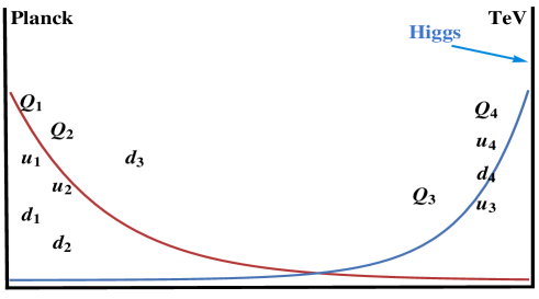
Figure 2: Typical geographic location of quarks in RS-4GEN (RS with a fourth family) such that large quark mass hierarchies and small mixing angles are generic. The Higgs boson and the heavier fermions (top and fourth generation quarks and charged leptons) are localized near the TeV brane, whereas light fermions are localized towards the Planck brane.

The mass matrices are

$${\bf m_{u}} = F_{Q}\ Y_{u}\ F_{u},$$ (15)

$$\ {\bf m_{d}} = F_{Q}\ Y_{d}\ F_{d},$$ (16)

where $F_{Q}$, $F_{u}$ and $F_{d}$ are $4\times 4$ diagonal matrices whose entries are given by the values at the IR brane of the corresponding zero-mode wave functions:

$$F_{Q}=\left(\begin{tabular}[]{cccc}$f_{Q_{1}}$&&\\ &$f_{Q_{2}}$&\\ &&$f_{Q_{3}}$\\ &&&$f_{Q_{4}}$\\ \end{tabular}\right),\ \ \ F_{u}=\left(\begin{tabular}[]{cccc}$f_{u_{1}}$&&\\ &$f_{u_{2}}$&\\ &&$f_{u_{3}}$\\ &&&$f_{u_{4}}$\\ \end{tabular}\right),\ \ \ F_{d}=\left(\begin{tabular}[]{cccc}$f_{d_{1}}$&&\\ &$f_{d_{2}}$&\\ &&$f_{d_{3}}$\\ &&&$f_{d_{4}}$\\ \end{tabular}\right).$$ (29)

The matrices $Y_{u}$ and $Y_{d}$ are the 5-dimensional Yukawa couplings, i.e. general $4\times 4$ complex matrices. Because most of the entries in the diagonal matrices $F_{q}$ are naturally hierarchical (for UV-localized fermions), the physical fermion mass matrices $m_{u}$ and $m_{d}$ will inherit their hierarchical structure independently of the nature of the true 5D Yukawa couplings $Y_{u}$ and $Y_{d}$, which can therefore contain all of its entries with similar size (of order 1) and have no definite flavor structure. This is the main idea behind scenarios of so-called flavor anarchy, which we consider also here, but applied to a four-family scenario. The introduction of the fourth family is simply realized by assuming that the new fermions are localized near the TeV brane, like the top quark, and therefore will be naturally heavy. Mixing angles should typically be small except among the heavy fermions where large mixings could be possible.

To diagonalize the mass matrices we use

$$\hskip 113.81102ptU_{Q_{u}}\ {\bf m_{u}}\ W_{u}^{\dagger} = {\bf m_{u}^{diag}},$$ (30)

$$\hskip 113.81102ptU_{Q_{d}}\ {\bf m_{d}}\ W_{d}^{\dagger} = {\bf m_{d}^{diag}}.$$ (31)

One can in fact obtain a relatively simple formulation of the rotation matrices $U_{Q_{u}}$, $U_{Q_{d}}$, $W_{u}$ and $W_{d}$ by expanding their entries in powers of ratios $f_{i}/f_{j}$, where $i<j$ and with $i=1,2$ and $j=1,2,3,4$. To proceed, we first define our notation. If ${\bf A}$ is an $n\times n$ matrix, then ${[\bf A]}_{ij}$ represents its $\{ij\}$ first order minor, i.e. the determinant of the $(n-1)\times(n-1)$ submatrix obtained by removing row $i$ and column $j$ from ${\bf A}$. We also use the notation ${\bf[A]}_{ij,\alpha\beta}$ to represent the $\{ij,\alpha\beta\}$ second order minor of ${\bf A}$, i.e. the determinant of the $(n-2)\times(n-2)$ submatrix obtained by removing rows $i$ and $\alpha$, and columns $j$ and $\beta$ from the matrix ${\bf A}$. Keeping only the leading terms, we obtain (see Casagrande:2008hr for the three family case):

[Yu]31∗[Yu]11∗fQ1fQ3−[Yu]11,32∗[Yu]11,22∗fQ2fQ3cQusQu−[Yu]41∗[Yu]11∗fQ1fQ4[Yu]11,42∗[Yu]11,22∗fQ2fQ4−s∗Quc∗Qu),fragments fragments fragmentssubscriptsuperscriptdelimited-[]subscript𝑌𝑢31subscriptsuperscriptdelimited-[]subscript𝑌𝑢11subscript𝑓subscript𝑄1subscript𝑓subscript𝑄3fragmentssubscriptsuperscriptdelimited-[]subscript𝑌𝑢1132subscriptsuperscriptdelimited-[]subscript𝑌𝑢1122subscript𝑓subscript𝑄2subscript𝑓subscript𝑄3fragmentscsubscript𝑄𝑢fragmentsssubscript𝑄𝑢fragmentssubscriptsuperscriptdelimited-[]subscript𝑌𝑢41subscriptsuperscriptdelimited-[]subscript𝑌𝑢11subscript𝑓subscript𝑄1subscript𝑓subscript𝑄4fragmentssubscriptsuperscriptdelimited-[]subscript𝑌𝑢1142subscriptsuperscriptdelimited-[]subscript𝑌𝑢1122subscript𝑓subscript𝑄2subscript𝑓subscript𝑄4fragmentsssubscript𝑄𝑢fragmentscsubscript𝑄𝑢\displaystyle\left(\begin{tabular}[]{cccc}$1\ $&$\vphantom{\frac{\int_{\int}}{\int_{\int_{\int}}}}\displaystyle\frac{[Y_{u}]_{{}_{21}}}{[Y_{u}]_{{}_{11}}}\ \frac{f_{Q_{1}}}{f_{Q_{2}}}\ \ $&${\cal U}^{Q_{u}}_{13}\ \ $&${\cal U}^{Q_{u}}_{14}\ \ $\\ $\vphantom{\frac{\int_{\int}}{\int_{\int_{\int}}}}-\displaystyle\frac{[Y_{u}]^{{}^{*}}_{{}_{21}}}{[Y_{u}]^{{}^{*}}_{{}_{11}}}\ \frac{f_{Q_{1}}}{f_{Q_{2}}}\ \ $&\ 1&${\cal U}^{Q_{u}}_{23}\ \ $&${\cal U}^{Q_{u}}_{24}\ \ $\\ $\ \ \vphantom{\frac{\int_{\int}}{\int_{\int_{\int}}}}\displaystyle\frac{[Y_{u}]^{{}^{*}}_{{}_{31}}}{[Y_{u}]^{{}^{*}}_{{}_{11}}}\ \frac{f_{Q_{1}}}{f_{Q_{3}}}\ $&$\vphantom{\frac{\int_{\int}}{\int_{\int_{\int}}}}-\displaystyle\frac{[Y_{u}]^{{}^{*}}_{{}_{11,32}}}{[Y_{u}]^{{}^{*}}_{{}_{11,22}}}\ \frac{f_{Q_{2}}}{f_{Q_{3}}}\ \ $&$c_{Q_{u}}$&$s_{Q_{u}}$\\ $\vphantom{\frac{\int_{\int}}{\int_{\int_{\int}}}}-\displaystyle\frac{[Y_{u}]^{{}^{*}}_{{}_{41}}}{[Y_{u}]^{{}^{*}}_{{}_{11}}}\ \frac{f_{Q_{1}}}{f_{Q_{4}}}\ $&$\ \ \vphantom{\frac{\int_{\int}}{\int_{\int_{\int}}}}\displaystyle\frac{[Y_{u}]^{{}^{*}}_{{}_{11,42}}}{[Y_{u}]^{{}^{*}}_{{}_{11,22}}}\ \frac{f_{Q_{2}}}{f_{Q_{4}}}\ \ $&$-s^{*}_{Q_{u}}$&$c^{*}_{Q_{u}}$\\ \end{tabular}\right),

$$U_{Q_{u}} = \left(\begin{tabular}[]{cccc}$1\ $&$\vphantom{\frac{\int_{\int}}{\int_{\int_{\int}}}}\displaystyle\frac{[Y_{u}]_{{}_{21}}}{[Y_{u}]_{{}_{11}}}\ \frac{f_{Q_{1}}}{f_{Q_{2}}}\ \ $&${\cal U}^{Q_{u}}_{13}\ \ $&${\cal U}^{Q_{u}}_{14}\ \ $\\ $\vphantom{\frac{\int_{\int}}{\int_{\int_{\int}}}}-\displaystyle\frac{[Y_{u}]^{{}^{*}}_{{}_{21}}}{[Y_{u}]^{{}^{*}}_{{}_{11}}}\ \frac{f_{Q_{1}}}{f_{Q_{2}}}\ \ $&\ 1&${\cal U}^{Q_{u}}_{23}\ \ $&${\cal U}^{Q_{u}}_{24}\ \ $\\ $\ \ \vphantom{\frac{\int_{\int}}{\int_{\int_{\int}}}}\displaystyle\frac{[Y_{u}]^{{}^{*}}_{{}_{31}}}{[Y_{u}]^{{}^{*}}_{{}_{11}}}\ \frac{f_{Q_{1}}}{f_{Q_{3}}}\ $&$\vphantom{\frac{\int_{\int}}{\int_{\int_{\int}}}}-\displaystyle\frac{[Y_{u}]^{{}^{*}}_{{}_{11,32}}}{[Y_{u}]^{{}^{*}}_{{}_{11,22}}}\ \frac{f_{Q_{2}}}{f_{Q_{3}}}\ \ $&$c_{Q_{u}}$&$s_{Q_{u}}$\\ $\vphantom{\frac{\int_{\int}}{\int_{\int_{\int}}}}-\displaystyle\frac{[Y_{u}]^{{}^{*}}_{{}_{41}}}{[Y_{u}]^{{}^{*}}_{{}_{11}}}\ \frac{f_{Q_{1}}}{f_{Q_{4}}}\ $&$\ \ \vphantom{\frac{\int_{\int}}{\int_{\int_{\int}}}}\displaystyle\frac{[Y_{u}]^{{}^{*}}_{{}_{11,42}}}{[Y_{u}]^{{}^{*}}_{{}_{11,22}}}\ \frac{f_{Q_{2}}}{f_{Q_{4}}}\ \ $&$-s^{*}_{Q_{u}}$&$c^{*}_{Q_{u}}$\\ \end{tabular}\right),$$ 1[Yu]21[Yu]11fQ1fQ2UQu13UQu14-[Yu]∗21[Yu]∗11fQ1fQ2 1UQu23UQu241[Yu]21[Yu]11fQ1fQ2UQu13UQu14-[Yu]∗21[Yu]∗11fQ1fQ2 1UQu23UQu24 (36)

[Yd]31∗[Yd]11∗fQ1fQ3−[Yd]11,32∗[Yd]11,22∗fQ2fQ3cQdsQd−[Yd]41∗[Yd]11∗fQ1fQ4[Yd]11,42∗[Yd]11,22∗fQ2fQ4−s∗Qdc∗Qd),fragments fragments fragmentssubscriptsuperscriptdelimited-[]subscript𝑌𝑑31subscriptsuperscriptdelimited-[]subscript𝑌𝑑11subscript𝑓subscript𝑄1subscript𝑓subscript𝑄3fragmentssubscriptsuperscriptdelimited-[]subscript𝑌𝑑1132subscriptsuperscriptdelimited-[]subscript𝑌𝑑1122subscript𝑓subscript𝑄2subscript𝑓subscript𝑄3fragmentscsubscript𝑄𝑑fragmentsssubscript𝑄𝑑fragmentssubscriptsuperscriptdelimited-[]subscript𝑌𝑑41subscriptsuperscriptdelimited-[]subscript𝑌𝑑11subscript𝑓subscript𝑄1subscript𝑓subscript𝑄4fragmentssubscriptsuperscriptdelimited-[]subscript𝑌𝑑1142subscriptsuperscriptdelimited-[]subscript𝑌𝑑1122subscript𝑓subscript𝑄2subscript𝑓subscript𝑄4fragmentsssubscript𝑄𝑑fragmentscsubscript𝑄𝑑\displaystyle\left(\begin{tabular}[]{cccc}$1\ $&$\vphantom{\frac{\int_{\int}}{\int_{\int_{\int}}}}\displaystyle\frac{[Y_{d}]_{{}_{21}}}{[Y_{d}]_{{}_{11}}}\ \frac{f_{Q_{1}}}{f_{Q_{2}}}\ \ $&${\cal U}^{Q_{d}}_{13}\ \ $&${\cal U}^{Q_{d}}_{14}\ \ $\\ $\vphantom{\frac{\int_{\int}}{\int_{\int_{\int}}}}-\displaystyle\frac{[Y_{d}]^{{}^{*}}_{{}_{21}}}{[Y_{d}]^{{}^{*}}_{{}_{11}}}\ \frac{f_{Q_{1}}}{f_{Q_{2}}}\ \ $&\ 1&${\cal U}^{Q_{d}}_{23}\ \ $&${\cal U}^{Q_{d}}_{24}\ \ $\\ $\ \ \vphantom{\frac{\int_{\int}}{\int_{\int_{\int}}}}\displaystyle\frac{[Y_{d}]^{{}^{*}}_{{}_{31}}}{[Y_{d}]^{{}^{*}}_{{}_{11}}}\ \frac{f_{Q_{1}}}{f_{Q_{3}}}\ $&$\vphantom{\frac{\int_{\int}}{\int_{\int_{\int}}}}-\displaystyle\frac{[Y_{d}]^{{}^{*}}_{{}_{11,32}}}{[Y_{d}]^{{}^{*}}_{{}_{11,22}}}\ \frac{f_{Q_{2}}}{f_{Q_{3}}}\ \ $&$c_{Q_{d}}$&$s_{Q_{d}}$\\ $\vphantom{\frac{\int_{\int}}{\int_{\int_{\int}}}}-\displaystyle\frac{[Y_{d}]^{{}^{*}}_{{}_{41}}}{[Y_{d}]^{{}^{*}}_{{}_{11}}}\ \frac{f_{Q_{1}}}{f_{Q_{4}}}\ $&$\ \ \vphantom{\frac{\int_{\int}}{\int_{\int_{\int}}}}\displaystyle\frac{[Y_{d}]^{{}^{*}}_{{}_{11,42}}}{[Y_{d}]^{{}^{*}}_{{}_{11,22}}}\ \frac{f_{Q_{2}}}{f_{Q_{4}}}\ \ $&$-s^{*}_{Q_{d}}$&$c^{*}_{Q_{d}}$\\ \end{tabular}\right),

$$U_{Q_{d}} = \left(\begin{tabular}[]{cccc}$1\ $&$\vphantom{\frac{\int_{\int}}{\int_{\int_{\int}}}}\displaystyle\frac{[Y_{d}]_{{}_{21}}}{[Y_{d}]_{{}_{11}}}\ \frac{f_{Q_{1}}}{f_{Q_{2}}}\ \ $&${\cal U}^{Q_{d}}_{13}\ \ $&${\cal U}^{Q_{d}}_{14}\ \ $\\ $\vphantom{\frac{\int_{\int}}{\int_{\int_{\int}}}}-\displaystyle\frac{[Y_{d}]^{{}^{*}}_{{}_{21}}}{[Y_{d}]^{{}^{*}}_{{}_{11}}}\ \frac{f_{Q_{1}}}{f_{Q_{2}}}\ \ $&\ 1&${\cal U}^{Q_{d}}_{23}\ \ $&${\cal U}^{Q_{d}}_{24}\ \ $\\ $\ \ \vphantom{\frac{\int_{\int}}{\int_{\int_{\int}}}}\displaystyle\frac{[Y_{d}]^{{}^{*}}_{{}_{31}}}{[Y_{d}]^{{}^{*}}_{{}_{11}}}\ \frac{f_{Q_{1}}}{f_{Q_{3}}}\ $&$\vphantom{\frac{\int_{\int}}{\int_{\int_{\int}}}}-\displaystyle\frac{[Y_{d}]^{{}^{*}}_{{}_{11,32}}}{[Y_{d}]^{{}^{*}}_{{}_{11,22}}}\ \frac{f_{Q_{2}}}{f_{Q_{3}}}\ \ $&$c_{Q_{d}}$&$s_{Q_{d}}$\\ $\vphantom{\frac{\int_{\int}}{\int_{\int_{\int}}}}-\displaystyle\frac{[Y_{d}]^{{}^{*}}_{{}_{41}}}{[Y_{d}]^{{}^{*}}_{{}_{11}}}\ \frac{f_{Q_{1}}}{f_{Q_{4}}}\ $&$\ \ \vphantom{\frac{\int_{\int}}{\int_{\int_{\int}}}}\displaystyle\frac{[Y_{d}]^{{}^{*}}_{{}_{11,42}}}{[Y_{d}]^{{}^{*}}_{{}_{11,22}}}\ \frac{f_{Q_{2}}}{f_{Q_{4}}}\ \ $&$-s^{*}_{Q_{d}}$&$c^{*}_{Q_{d}}$\\ \end{tabular}\right),$$ 1[Yd]21[Yd]11fQ1fQ2UQd13UQd14-[Yd]∗21[Yd]∗11fQ1fQ2 1UQd23UQd241[Yd]21[Yd]11fQ1fQ2UQd13UQd14-[Yd]∗21[Yd]∗11fQ1fQ2 1UQd23UQd24 (41)

where, in particular, we have

$${\cal U}^{Q_{d}}_{23} = c_{Q_{d}}\frac{f_{Q_{2}}}{f_{Q_{3}}}\ \frac{[Y_{d}]_{{}_{11,32}}}{[Y_{d}]_{{}_{11,22}}}\ +s^{*}_{Q_{d}}\frac{f_{Q_{2}}}{f_{Q_{4}}}\ \frac{[Y_{d}]_{{}_{11,42}}}{[Y_{d}]_{{}_{11,22}}},$$ (42)

$${\cal U}^{Q_{d}}_{13} = c_{Q_{d}}\frac{f_{Q_{1}}}{f_{Q_{3}}}\ \frac{[Y_{d}]_{{}_{21,32}}}{[Y_{d}]_{{}_{11,22}}}\ +s^{*}_{Q_{d}}\frac{f_{Q_{1}}}{f_{Q_{4}}}\ \frac{[Y_{d}]_{{}_{21,42}}}{[Y_{d}]_{{}_{11,22}}},$$ (43)

where we used properties of the minors. These are needed to compute the $V_{CKM}$ elements $V_{cb}$ and $V_{ub}$. Due to the mass hierarchy $m_{b}\ll m_{b^{\prime}}$, we also have the simple expansions:

$$c_{Q_{d}}=v_{4}\ f_{Q_{4}}f_{d_{4}}|Y^{d}_{44}|/m_{b^{\prime}}\ \ \ \ {\rm and}\ \ \ \ s^{*}_{Q_{d}}=v_{4}\ f_{Q_{3}}f_{d_{4}}{Y^{d}_{34}}^{*}/m_{b^{\prime}}\ e^{i\arg{(Y^{d}_{44})}}.$$ (44)

Since

$$V_{CKM}=U_{Q_{u}}^{+}U_{Q_{d}},$$ (45)

we can find expressions for $V_{us}$, $V_{cb}$ and $V_{ub}$:

$$V_{us}=\frac{f_{Q_{1}}}{f_{Q_{2}}}\left(\frac{[Y_{d}]_{{}_{21}}}{[Y_{d}]_{{}_{11}}}-\frac{[Y_{u}]_{{}_{21}}}{[Y_{u}]_{{}_{11}}}\right),$$ (46)

and

$$V_{cb}=c_{Q_{d}}\frac{f_{Q_{2}}}{f_{Q_{3}}}\ \left(\frac{[Y_{d}]_{{}_{11,32}}}{[Y_{d}]_{{}_{11,22}}}\ -\frac{[Y_{u}]_{{}_{11,32}}}{[Y_{u}]_{{}_{11,22}}}\ \right)\ +\ s^{*}_{Q_{d}}\frac{f_{Q_{2}}}{f_{Q_{4}}}\left(\frac{[Y_{d}]_{{}_{11,42}}}{[Y_{d}]_{{}_{11,22}}}\ -\frac{[Y_{u}]_{{}_{11,42}}}{[Y_{u}]_{{}_{11,22}}}\ \right),$$ (47)

and

$$V_{ub} =c_{Q_{d}}\frac{f_{Q_{1}}}{f_{Q_{3}}}\left(\frac{[Y_{u}]_{{}_{31}}}{[Y_{u}]_{{}_{11}}}+\frac{[Y_{d}]_{{}_{21,32}}}{[Y_{d}]_{{}_{11,22}}}-\frac{[Y_{u}]_{{}_{21}}}{[Y_{u}]_{{}_{11}}}\frac{[Y_{d}]_{{}_{11,32}}}{[Y_{d}]_{{}_{11,22}}}\right)\!$$ (48)

$$+s^{*}_{Q_{d}}\frac{f_{Q_{1}}}{f_{Q_{4}}}\left(\frac{[Y_{u}]_{{}_{41}}}{[Y_{u}]_{{}_{11}}}+\frac{[Y_{d}]_{{}_{21,42}}}{[Y_{d}]_{{}_{11,22}}}-\frac{[Y_{u}]_{{}_{21}}}{[Y_{u}]_{{}_{11}}}\frac{[Y_{d}]_{{}_{11,42}}}{[Y_{d}]_{{}_{11,22}}}\right).\ \ \$$

It is clear that if the 5D Yukawa matrix elements are all of order 1, then the observed hierarchies among the CKM elements can still be explained by hierarchies among the $f_{i}$ parameters. The explicit dependence on the 5D Yukawa couplings gives a more precise prediction for the mixing angles, which will be quite useful when looking for phenomenologically viable points in parameter space. The results of such a scan are presented in the next subsection.

III.2 Tree level Higgs FCNC couplings

We now extend the one-family results presented in section II to the case of four generations. To leading order in Yukawa couplings, the SM fermion mass matrix is

$$\hat{m}^{d}=\hat{F}_{Q}\hat{Y}_{1}^{5D}\hat{F}_{d}\ \ {v_{4}},$$ (49)

where $\hat{}$ means a $4\times 4$ matrix in flavor space. The misalignment in flavor space between the fermion mass matrix and the Yukawa coupling matrix is defined as

$$\hat{\Delta}^{d}=\hat{m}^{d}-v_{4}\ \hat{y}_{4}^{d},$$ (50)

where $\hat{y}_{4}^{d}$ is the 4D effective coupling matrix between the physical scalar Higgs and the quarks.

Similarly to the one family case, the misalignment can be separated into two components, $\hat{\Delta}^{d}_{1}+\hat{\Delta}^{d}_{2}$, with (see toharia1 )

$$\hat{\Delta}^{d}_{1} = \frac{2}{3}\ \hat{m}^{d}\frac{1}{\hat{F}_{d}}(\hat{Y}^{5D}_{2})^{\dagger}\frac{1}{\hat{F}_{Q}}\hat{m}^{d}\ \left({v_{4}^{3}R^{\prime 2}}\right),$$ (51)

and

$$\hat{\Delta}^{d}_{2}=\hat{m}^{d}\left(\hat{m}^{d\dagger}\hat{K}(c_{q})+\hat{K}(-c_{d})\hat{m}^{d\dagger}\right)\hat{m}^{d}\ R^{\prime 2}$$ (52)

The crucial observation is that $\hat{m}^{d}$ and $\hat{\Delta}^{d}$ are generally not aligned in flavor space. Thus when we diagonalize the quark mass matrix with a bi-unitary transformation $\hat{m}^{d}\rightarrow U^{\dagger}_{Q_{L}}\hat{m}^{d}W_{d}$, the Yukawa couplings will not be diagonal. To be more specific, in models of flavor anarchy, we have

$$(U_{Q_{d}},W_{d})_{i,j}\sim\frac{f_{Q_{i},d_{i}}}{f_{Q_{j},d_{j}}}\qquad\text{for}\quad{i<j}.$$ (53)

Then the off-diagonal Yukawa coupling will be dominated by

$$\hat{Y}^{\text{off}}_{ij} = -(U^{\dagger}_{d_{L}}\hat{\Delta}^{d}W_{d_{R}})_{ij}\frac{1}{v_{4}}\sim\frac{2}{3}f_{Q_{i}}\bar{Y}^{3}f_{d_{j}}v_{4}^{2}R^{\prime 2},$$ (54)

where $\bar{Y}$ is the typical value of the dimensionless 5D Yukawa coupling.

Since the Higgs couplings will now contain off-diagonal entries, we must choose a convenient parametrization for them. A common choice is to normalize the couplings with the fermion masses and write the Higgs Yukawa couplings as

$${\cal{L}}_{HFV}=a^{d}_{ij}\sqrt{\frac{m^{d}_{i}m^{d}_{j}}{v_{4}^{2}}}H\bar{d}_{L}^{i}d_{R}^{j}+h.c.+(d\leftrightarrow u).$$ (55)

III.2.1 Analytical estimates of Higgs FCNC couplings in Flavor Anarchy

In this section, following the same procedure as in toharia1 , we estimate the off-diagonal couplings of Higgs boson to SM fermions and then we do a numerical scan over anarchical Yukawa couplings to support our estimates.

We use Eqs. (53) and (54) to estimate the sizes of $a^{u,d}_{ij}$. For example, we have

$$a^{d}_{12} \sim \frac{2}{3}f_{Q_{1}}\bar{Y}^{3}f_{d_{2}}v_{4}^{2}R^{\prime 2}\sqrt{\frac{v_{4}^{2}}{m_{s}m_{d}}}\sim\frac{2}{3}\lambda\bar{Y}^{2}v_{4}^{2}R^{\prime 2}\sqrt{\frac{m_{s}}{m_{d}}},$$ (56)

where $\lambda\approx 0.22$ is the Wolfenstein parameter, and we used $f_{q_{1}}/f_{q_{2}}\sim(U_{d_{L}})_{12}\sim(V_{CKM})_{12}\sim\lambda$. We can find the other $a^{u,d}_{ij}$ in similar fashion. We obtain:

$$a^{d}_{ij}\sim\delta_{ij}-\frac{2}{3}\bar{Y}^{2}v_{4}^{2}R^{\prime 2}\left(\begin{array}[]{cccc}1&\lambda\sqrt{\frac{m_{s}}{m_{d}}}&\lambda^{3}\sqrt{\frac{m_{b}}{m_{d}}}&\lambda^{3}\sqrt{\frac{m_{b^{\prime}}}{m_{d}}}\\ \frac{1}{\lambda}\sqrt{\frac{m_{d}}{m_{s}}}&4&\lambda^{2}\sqrt{\frac{m_{b}}{m_{s}}}&\lambda^{2}\sqrt{\frac{m_{b^{\prime}}}{m_{s}}}\\ \frac{1}{\lambda^{3}}\sqrt{\frac{m_{d}}{m_{b}}}&\frac{1}{\lambda^{2}}\sqrt{\frac{m_{s}}{m_{b}}}&12&\sqrt{\frac{m_{b^{\prime}}}{m_{b}}}\\ \frac{1}{\lambda^{3}}\sqrt{\frac{m_{d}}{m_{b^{\prime}}}}&\frac{1}{\lambda^{2}}\sqrt{\frac{m_{s}}{m_{b^{\prime}}}}&\sqrt{\frac{m_{b}}{m_{b^{\prime}}}}&12\end{array}\right),$$ (61)

$$a^{u}_{ij}\sim\delta_{ij}-\frac{2}{3}\bar{Y}^{2}v_{4}^{2}R^{\prime 2}\left(\begin{array}[]{cccc}1&\lambda\sqrt{\frac{m_{c}}{m_{u}}}&\lambda^{3}\sqrt{\frac{v_{4}^{2}}{m_{t}m_{u}}}&\lambda^{3}\sqrt{\frac{v_{4}^{2}}{m_{t^{\prime}}m_{u}}}\\ \frac{1}{\lambda}\sqrt{\frac{m_{u}}{m_{c}}}&4&\lambda^{2}\sqrt{\frac{v^{2}_{4}}{m_{t}m_{c}}}&\lambda^{2}\sqrt{\frac{v^{2}_{4}}{m_{t^{\prime}}m_{c}}}\\ \frac{1}{\lambda^{3}}\sqrt{\frac{m_{u}}{m_{t}}}&\frac{1}{\lambda^{2}}\sqrt{\frac{m_{c}}{m_{t}}}&16&\sqrt{\frac{m_{t^{\prime}}m_{t}}{v_{4}^{2}}}\\ \frac{1}{\lambda^{3}}\sqrt{\frac{m_{u}}{m_{t^{\prime}}}}&\frac{1}{\lambda^{2}}\sqrt{\frac{m_{c}}{m_{t^{\prime}}}}&\sqrt{\frac{v_{4}^{2}}{m_{t^{\prime}}m_{t}}}&16\end{array}\right).$$ (66)

The effect clearly decouples since it depends on $R^{\prime 2}\sim\frac{1}{M_{KK}^{2}}$. Taking the typical Yukawa size $\bar{Y}=2$ and $1/R^{\prime}=1500$ GeV, and using the known SM masses evaluated at the KK scale, along with $m_{t^{\prime}}=400$ GeV and $m_{b^{\prime}}=350$ GeV, one can obtain the typical values of these couplings:

$$a^{d}_{ij}\sim\left(\begin{array}[]{cccc}0.96&0.03&0.01&0.14\\ 0.04&0.86&0.01&0.15\\ 0.13&0.19&0.57&0.45\\ 0.01&0.007&0.003&0.57\end{array}\right),$$ (71)

$$a^{u}_{ij}\sim\left(\begin{array}[]{cccc}0.96&0.16&0.15&0.09\\ 0.008&0.86&0.04&0.02\\ 0.01&0.04&0.42&0.05\\ 0.007&0.03&0.003&0.42\end{array}\right).$$ (76)

Note that the results presented here are just estimates for the size of $a^{u,d}_{ij}$, which come without sign or phases. However, we observe that for the third and fourth generation quarks, the corrections to the diagonal Yukawa couplings are always negative (suppressions) if $Y_{1}=Y_{2}$ and are larger than the previous estimates. This point was argued in toharia1 and we address it again the next subsection for completeness.

An interesting feature of these matrices is the asymmetry of $a^{d}_{ij}$ in the $b_{L}b_{R}^{\prime}$ and $b_{L}^{\prime}b_{R}$ entries, asymmetry not shared by the up-quark matrix $a^{u}_{ij}$. These would produce an asymmetry in the decays, as well as in the shift of the the vertex functions $g^{b}_{L}$, $g^{b}_{R}$ for $Z\to b\bar{b}$. This asymmetry will be typical to the $(34-43)$ entries and thus non-universal. We expect the same feature in the charged lepton mass matrix.

III.2.2 Numerical results for Higgs FCNC couplings

In order to obtain a better prediction of the typical size of the off-diagonal Yukawa couplings, and to compare with the previous estimates we perform a scan in parameter space. The results should be in general consistent with the rough estimates of Eqs. (71) and (76). Some differences observed can nevertheless be explained, (see also toharia1 ) so that one can still be confident in the generic size of the flavor violating couplings predicted in the flavor anarchy paradigm in RS type scenarios with four generations.

We proceed as follows:

• We fix $m_{t^{\prime}}=400$ GeV and $m_{b^{\prime}}=350$ GeV as well as SM quark masses at the KK scale, taken to be $m_{t}=140$ GeV, $m_{b}=2.2$ GeV, $m_{c}=0.55$ GeV, $m_{s}=5\times 10^{-2}$ GeV, $m_{u}=1.5\times 10^{-3}$ GeV, $m_{d}=3.0\times 10^{-3}$ GeV. We take the KK scale as ${R^{\prime}}^{-1}=1500$ GeV.

• Then we generate random complex entries for $Y_{u}$ and $Y_{d}$, such that $|Y_{i}|\in[0.3,3.5]$. We also generate random $f_{Q_{4}}$ such that $f_{Q_{4}}\sim{\cal O}(1)$.

• We then obtain $f_{Q_{3}}$ from $|V_{ub}|/|V_{us}|/|V_{cb}|$, $\ f_{Q_{2}}$ from $|V_{ub}|/|V_{us}|\$ and $\ f_{Q_{1}}$ from $|V_{us}|$ (see Eqs. (46), (47) and (48)).

• We then obtain the right-handed down quark entries $f_{d_{4}}$ from $m_{b^{\prime}}$.

• Similarly for the up right-handed matrix entries, we obtain $f_{u_{1}}$, $f_{u_{2}}$, $f_{d_{1}}$, $f_{d_{2}}$ and $f_{d_{3}}$ from $m_{u},m_{c},m_{d},m_{s}$ and $m_{b}$. We also obtain $f_{u_{3}}$ and $f_{u_{4}}$ from $m_{t}$ and $m_{t^{\prime}}$.

• Finally we check that the generated $Y_{u}$ and $Y_{d}$ along with the obtained $\hat{F}_{q}$, $\hat{F}_{u}$ and $\hat{F}_{d}$ do indeed produce the observed masses and mixings of the SM. If so we keep the point in parameter space and continue until we obtain 1000 points which satisfy all constraints.

• For each acceptable point, we use Eqs. (51) and (52) to compute the flavor violating Higgs Yukawa couplings, parametrized by the $a_{ij}$’s as defined in Eq. (55).

We present the results of the scan as follows: we give the 25% quantile and the 75% quantile of the obtained couplings. This means that 50% of our acceptable points contain a coupling in between the quoted values. Also it means that 25% of the generated points predict higher values than the range quoted, while 25% of the points predict lower values than the range quoted.

We find the following ranges for $a^{d}_{ij},\ a^{u}_{ij}$ matrix couplings

$$a^{d}_{ij}\sim\left(\begin{array}[]{cccc}0.919-0.987&0.025-0.081&0.011-0.044&0.130-0.532\\ 0.049-0.148&0.827-0.934&0.0.017-0.059&0.249-0.934\\ 0.140-0.470&0.142-0.446&0.620-0.819&0.873-2.508\\ 0.018-0.061&0.017-0.058&0.008-0.120&0.375-0.643\end{array}\right),$$ (81)

$$a^{u}_{ij}\sim\left(\begin{array}[]{cccc}0.927-1.000&0.089-0.364&0.091-0.410&0.139-0.612\\ 0.015-0.052&0.816-0.949&0.065-0.197&0.092-0.300\\ 0.019-0.068&0.071-0.236&0.545-0.772&0.127-0.343\\ 0.0167-0.062&0.060-0.191&0.064-0.168&0.403-0.651\end{array}\right),$$ (86)

to be compared with the rough estimates Eqs. (71) and (76).

III.2.3 Cumulative effect on diagonal Yukawa couplings when $Y_{1}=Y_{2}$

We observe that the rough estimates are slightly smaller than the results of the scan, specially for the third and fourth generation couplings. This was already pointed out in toharia1 for the three generation case. The argument given is that due to the presence of a fourth generation some of the coefficients will be different and typically the cumulative effect will be larger.

We assume that $Y_{1}=Y_{2}$ and consider for example the element ${(33)}$ of the Yukawa coupling in the up quark sector, i.e.

$$a_{tt}-1 = -\frac{2{R^{\prime}}^{2}}{3m_{t}}\left[U^{\dagger}_{Q_{u}}\hat{m}^{u}\frac{1}{\hat{F}_{u}^{2}}\hat{m}^{u\dagger}\frac{1}{\hat{F}_{Q}^{2}}\hat{m}^{u}W_{u}\right]_{33}$$ (87)

$$= -\frac{2{R^{\prime}}^{2}}{3m_{t}}\left(m_{u}^{diag}\right)_{33}\left(W^{\dagger}_{u}\frac{1}{\hat{F}_{u}^{2}}W_{u}\right)_{3j}\left(m_{u}^{diag}\right)_{jj}\left(U^{\dagger}_{Q_{u}}\frac{1}{\hat{F}_{Q}^{2}}U_{Q_{u}}\right)_{j3}\left(m_{u}^{diag}\right)_{33}.$$

First let’s look at the contribution to $a_{tt}$ when the $j$ index is equal to 3 (i.e. in the middle mass matrix $m_{u}^{diag}$ is $m_{t}$). In this case, there will be 16 terms in phase, each proportional to $-\frac{2{R^{\prime}}^{2}\bar{Y}^{2}v_{4}^{2}}{3}$, and it is important to realize that every one of them will be real and negative, because $(W^{\dagger}_{u}\frac{1}{\hat{F}_{u}^{2}}W_{u})_{33}\geq 0$. When $j=2$ $(m_{u}^{diag}=m_{c})$ there will be 2 terms $\sim\frac{2{R^{\prime}}^{2}\bar{Y}^{2}v_{4}^{2}}{3}$ but every one of them will have generically a random complex phase (the 14 remaining terms are much smaller). For $j=1$ $(m_{u}^{diag}=m_{u})$ there is only one term $\sim\frac{2{R^{\prime}}^{2}\bar{Y}^{2}v_{4}^{2}}{3}$ contributing, with the rest 15 terms being again suppressed. So, summing, the dominant contribution to $a_{tt}$ will consist of 19 terms, 16 of which are negative and the rest 3 have random complex phases. Generically each of these terms are of the same size $\sim\frac{2{R^{\prime}}^{2}\bar{Y}^{2}v^{2}}{3}$ so from a statistical argument, $a_{tt}-1$ should receive a negative contribution $\sim-16\left(\frac{2{R^{\prime}}^{2}\bar{Y}^{2}v^{2}}{3}\right)$. This cumulative effect is confirmed by the numerical scan.

One can perform the same analysis for the rest of elements of the Yukawa matrix, including the off diagonal ones, and realize that typically there are a number of aligned terms in each case which enhances the naive estimate by an ${\cal O}(1)$ factor (which can be estimated also). This fact gives us confidence that both our scan and our estimates are consistent and that our numerical results predict correctly in this scenario the generic size of the flavor violating couplings in the Higgs sector.

III.2.4 Higgs FCNC couplings in the lepton sector

We proceed in a similar fashion to evaluate Higgs flavor violation in the lepton sector. The difficulty with the lepton sector is that mixing matrices are not well-established here. The neutrinos can be either Dirac or Majorana, the charged lepton mixing matrix (PMNS) is not as well established as the CKM matrix, and there are several mechanisms to explain the large mixing angles and light masses for the neutrinos (see for example Perez:2008ee ; Agashe:2009tu ). For all cases, the Lagrangian can then be parametrized as:

$${\cal{L}}_{HFV}=a^{l}_{ij}\sqrt{\frac{m^{l}_{i}m^{l}_{j}}{v_{4}^{2}}}H\bar{L}^{i}e^{j}+h.c.$$ (88)

Following Agashe:2009tu ; toharia1 , we analyze two types of scenarios. Depending on the neutrino model, the left-handed charged lepton profiles can be either hierarchical and UV localized, or similar and UV localized. The profiles of the right-handed charged leptons are always hierarchical and localized near the UV brane. We outline both cases below.

• (A) In the case where the left-handed and right-handed profiles are hierarchical, they satisfy the following relations:

  $$f_{L}^{i}f_{e}^{i}\sim\frac{m_{i}^{l}}{\bar{Y}v_{4}},\qquad(O_{L,e})^{i,j}\sim\frac{f_{L,e}^{i}}{f_{L,e}^{j}},\qquad~{}i<j.$$ (89)

  where $f_{L,e}$ are profiles of the left-handed and right-handed fields and $(O_{L,e})^{i,j}$ is the intergenerational mixing. Then the $a^{l}_{ij}$ become:

  $$a^{l}_{ij}\sim\frac{2}{3}\bar{Y}^{2}(v_{4}^{2}{R^{\prime}}^{2})\sqrt{\frac{f_{L}^{i}f_{e}^{j}}{f_{L}^{j}f_{e}^{i}}}.$$ (90)

  This $a_{ij}^{l}$ are maximal when $\displaystyle\frac{f_{L}^{i}}{f_{L}^{j}}\sim\frac{f_{e}^{i}}{f_{e}^{j}}\sim\sqrt{\frac{m^{l}_{i}}{m_{j}^{l}}}$, i.e., when the hierarchy of charged lepton masses gets equal contributions from the left-handed and right-handed fields.

• (B) If right-handed profiles are hierarchical and left-handed profiles are similar, $f_{L}^{1}\sim f_{L}^{2}\sim f_{L}^{3}$, the profiles satisfy the following relations:

  $$f^{i}_{L}f_{e}^{i} \sim \frac{m^{l}_{i}}{\bar{Y}v_{4}},\qquad\frac{f_{L}^{i}}{f_{L}^{j}}\sim O(1),\qquad\frac{f_{e}^{i}}{f_{e}^{j}}\sim\frac{m_{i}^{l}}{m_{j}^{l}},\qquad~{}i<j,$$ (91)

  and the the parameter $a^{l}_{ij}$ becomes:

  $$a^{l}_{ij}\sim\frac{2}{3}\bar{Y}^{2}(v_{4}^{2}{R^{\prime}}^{2})\sqrt{\frac{f_{e}^{j}}{f_{e}^{i}}}.$$ (92)

  These flavor violating Higgs Yukawa couplings to leptons can also lead to interesting collider signals for the decays of the fourth generation leptons, as discussed in the next section.

III.3 Tree Level $Z^{0}$ flavor violating couplings

FCNC couplings of the $Z^{0}$ boson have been studied before in the context of warped scenarios with 3 generations Casagrande:2008hr . These couplings arise basically from two sources. First, the bulk profiles of the lowest-lying massive gauge bosons (the SM $Z^{0}$ and $W^{0}$) are not flat, yielding non-trivial and non-universal overlap integrals with the fermion profiles. Second, even if the $Z^{0}$ and $W^{0}$ profiles were flat, there would still be a non-universal correction to these couplings due to misalignments in the fermion kinetic terms. In fact the correction has the exact same origin as the misalignment $\hat{\Delta}^{d}_{2}$ in the Higgs sector shown in Eq. (52).

For light quarks, the first source of misalignment dominates due to Yukawa suppression of the fermion kinetic term misalignments. But for heavier quarks, and specially fourth generation quarks, this last source of flavor should dominate and this is the one we consider in the following.

We can write the couplings of fermions with $Z^{0}$ as:

$${\cal{L}}_{Z}=\left[g_{L}\ \delta_{ij}+\left(\hat{\delta}_{g_{L}}\right)_{ij}\right]\bar{d}_{L}^{i}Z\!\!\!\!/\ d_{L}^{j}\ \ +\ \ \left[g_{R}\ \delta_{ij}+\left(\hat{\delta}_{g_{R}}\right)_{ij}\right]\bar{d}_{R}^{i}Z\!\!\!\!/\ d_{R}^{j}\ +\ (d\leftrightarrow u),$$ (93)

where $\displaystyle g_{L}=\frac{g}{\cos{\theta}_{W}}(T_{3}-Q\sin{\theta_{W}}^{2})$ and $\displaystyle g_{R}=\frac{g}{\cos{\theta_{W}}}Q\sin{\theta_{W}}^{2}$ are the usual diagonal SM couplings with $g$ the $SU(2)_{L}$ coupling constant, and $Q$ and $T_{3}$ the charge and the isospin of the quark in question. The corrections coming from the kinetic term misalignment are, for the down quarks,

$$\hat{\delta}^{kin}_{g_{L}} = -\frac{gT^{d}_{3}}{\cos\theta_{W}}\ \ \hat{m}^{d\dagger}\hat{K}_{c_{q}}\hat{m}^{d}\ R^{\prime 2},$$ (94)

$$\hat{\delta}^{kin}_{g_{R}} = \ \ \frac{gT^{d}_{3}}{\cos\theta_{W}}\ \ \hat{m}^{d}\hat{K}_{c_{d}}\hat{m}^{d\dagger}\ R^{\prime 2}.$$ (95)

where $\hat{m}^{d}$ is the fermion mass matrix before diagonalization, ${R^{\prime}}^{-1}$ is the KK scale and $\hat{K}$ is a diagonal matrix whose entries $K(c)$ were defined in Eq. (14). Upon diagonalization of the fermion mass matrix in order to go to the physical basis, these corrections will not be diagonal and will produce flavor violating coupling for the $Z^{0}$ boson. The same mechanism applies in the up-sector.

Once in the physical basis, we can parametrize the off-diagonal quark couplings in the Lagrangian by $\left(a_{L}^{u,d}\right)_{ij}$ and $\left(a_{R}^{u,d}\right)_{ij}$, with

$${\cal{L}}_{ZFV}=-\frac{gT^{d}_{3}}{\cos\theta_{W}}\left[\left(a_{L}^{d}\right)_{ij}\bar{d}_{L}^{i}Z\!\!\!\!/\ d_{L}^{j}-\left(a_{R}^{d}\right)_{ij}\bar{d}_{R}^{i}Z\!\!\!\!/\ d_{R}^{j}\right]+(d\leftrightarrow u).$$ (96)

The $Z^{0}$ FCNC couplings $\left(a_{L}^{u,d}\right)_{ij}$, $\left(a_{R}^{u,d}\right)_{ij}$ can then be obtained from the same scan used to obtain numerical values for the Higgs FCNC couplings. For example, for the $(43)$ entries in the up and down sector, we find typical ranges

$$(a^{u}_{L})_{43}={0.00350-0.0176},\ \ \ \ (a^{u}_{R})_{43}={0.0274-0.0952},$$ (97)

$$(a^{d}_{L})_{43}={0.00356-0.0161},\ \ \ \ (a^{d}_{R})_{43}={0.0209-0.0830}.$$ (98)

To obtain these values we followed the same procedure explained previously in the subsection “Numerical results for Higgs FCNC couplings”.

IV Phenomenology

IV.1 Bounds on Higgs-mediated FCNC couplings

The off-diagonal Higgs Yukawa couplings induce FCNC, which affect many low energy observables and also give possible signatures at colliders. In this section, we discuss first bounds on Higgs flavor violation coming from tree-level processes $\Delta F=2$, such as $K-\bar{K}$, $B-\bar{B}$, $D-\bar{D}$ mixing. We then study the effects on loop processes, such as $b$ and $t$ flavor-changing decays, as well as on $Z\to b\bar{b},\ \tau^{+}\tau^{-}$. The radiative processes are enhanced due to heavy quarks in the loop, and strong off-diagonal Yukawa couplings.

IV.1.1 Tree-level processes

The $\Delta F=2$ process can be described by the general Hamiltonian UTfit ; BurasWeakHamiltonian

$${\cal H}_{eff}^{\Delta F=2}=\sum_{a=1}^{5}C_{a}Q_{a}^{q_{i}q_{j}}+\sum_{a=1}^{3}\tilde{C}_{a}\tilde{Q}_{a}^{q_{i}q_{j}},$$ (99)

with

$$Q_{1}^{q_{i}q_{j}} = \bar{q}^{\alpha}_{jL}\gamma_{\mu}q_{iL}^{\alpha}\bar{q}^{\beta}_{jL}\gamma^{\mu}q^{\beta}_{iL},\quad Q_{2}^{q_{i}q_{j}}=\bar{q}^{\alpha}_{jR}q_{iL}^{\alpha}\bar{q}^{\beta}_{jR}q_{iL}^{\beta},\quad Q_{3}^{q_{i}q_{j}}=\bar{q}^{\alpha}_{jR}q_{iL}^{\beta}\bar{q}_{jR}^{\beta}q_{iL}^{\alpha},$$ (100)

$$Q_{4}^{q_{i}q_{j}} = \bar{q}^{\alpha}_{jR}q_{iL}^{\alpha}\bar{q}_{jL}^{\beta}q_{iR}^{\beta},\quad Q_{5}^{q_{i}q_{j}}=\bar{q}^{\alpha}_{jR}q_{iL}^{\beta}\bar{q}^{\beta}_{jL}q_{iR}^{\alpha},$$

where $\alpha,\beta$ are color indices. The operators $\tilde{Q}_{a}$ are obtained from $Q_{a}$ by exchange $L\leftrightarrow R$. For $K-\bar{K}$ , $B_{d}-\bar{B}_{d}$, $B_{s}-\bar{B}_{s}$, $D-\bar{D}$ mixing, $q_{i}q_{j}=sd$, $bd$, $bs$ and $uc$ respectively.

Exchange of the flavor-violating Higgs bosons gives rise to new contribution to $C_{2}$, $\tilde{C}_{2}$ and $C_{4}$ operators BlankedeltaF2 . These contributions have been included in toharia1 , and the basic bounds on the coefficients are not altered. We present them here, for completeness, in a more general fashion, with no relation to the possible numerical values of the entries in the Higgs Yukawa mass matrix. We use the model-independent bounds on BSM contributions as in UTfit , and present coupled constraints on the Higgs flavor violating Yukawa couplings parametrized by the $a_{ij}$ couplings and the Higgs mass $m_{h}$.

• $K^{0}-\bar{K}^{0}$ mixing

  The coefficients $C_{2}$, $\tilde{C}_{2}$ and $C_{4}$ will set limits on the real and imaginary of the Yukawa couplings $a^{d}_{12},\ a^{d}_{21}$, and their product. Specifically, for the values of parameters used in the previous sections, we obtain, from $\Delta M_{K}$, respectively:

  $$|(a_{12}^{d})|\left(\frac{400~{}{\rm GeV}}{m_{h}}\right)\leq 0.62,\quad|(a_{21}^{d})|\left(\frac{400~{}{\rm GeV}}{m_{h}}\right)\leq 0.62,$$ (101)

  $$|(a_{12}^{d}a_{21}^{d})|\left(\frac{400~{}{\rm GeV}}{m_{h}}\right)^{2}\leq(0.35)^{2}.$$

  The bounds obtained from $\epsilon_{K}$ are very stringent, and restrict the phases of the off-diagonal Higgs Yukawa couplings:

  $$\text{Im}(a_{12}^{d})^{2}\left(\frac{400~{}{\rm GeV}}{m_{h}}\right)^{2}\leq\left(4.6\times 10^{-2}\right)^{2},\quad\text{Im}(a_{21}^{d})^{2}\left(\frac{400~{}{\rm GeV}}{m_{h}}\right)^{2}\leq\left(4.6\times 10^{-2}\right)^{2}$$

  $$\text{Im}(a_{12}^{d}a_{21}^{d})\left(\frac{400~{}{\rm GeV}}{m_{h}}\right)^{2}\leq\left(2.2\times 10^{-2}\right)^{2}$$ (102)

• $D^{0}-\bar{D}^{0}$ mixing

  The $D^{0}-\bar{D}^{0}$ mixing constrains the ${(12,\ 21)}$ off-diagonal entries in the up-quark flavor changing mixings.

  $$|(a_{12}^{u})|\left(\frac{400~{}{\rm GeV}}{m_{h}}\right)\leq 0.71,\quad|(a_{21}^{u})|\left(\frac{400~{}{\rm GeV}}{m_{h}}\right)\leq 0.71,$$

  $$|(a_{12}^{u}a_{21}^{u})|\left(\frac{400~{}{\rm GeV}}{m_{h}}\right)^{2}\leq\left(0.47\right)^{2}.$$ (103)

• $B^{0}_{d}-\bar{B}^{0}_{d}$ mixing

  The mass mixing in the $B^{0}_{d}-\bar{B}^{0}_{d}$ is fairly constrained, resulting in bounds on the ${(13,\ 31)}$ entries in the down-quark flavor changing mixings.

  $$|(a_{13}^{d})|\left(\frac{400~{}{\rm GeV}}{m_{h}}\right)\leq 0.54,\quad|(a_{31}^{d})|\left(\frac{400~{}{\rm GeV}}{m_{h}}\right)\leq 0.54,$$

  $$|(a_{13}^{d}a_{31}^{d})|\left(\frac{400~{}{\rm GeV}}{m_{h}}\right)^{2}\leq\left(0.35\right)^{2}.$$ (104)

• $B^{0}_{s}-\bar{B}^{0}_{s}$ mixing

  The mass mixing in the $B^{0}_{s}-\bar{B}^{0}_{s}$ is less restricted than in the $B_{d}^{0}$ sector, resulting in bounds on the ${(23,\ 32)}$ entries in the down-quark flavor changing mixings. At first, these bounds may not appear useful; however, one must note that the matrix entries $a_{ij}$ are not otherwise constrained (e.g., by unitarity).

  $$|(a_{23}^{d})|\left(\frac{400~{}{\rm GeV}}{m_{h}}\right)\leq 1.1,\quad|(a_{32}^{d})|\left(\frac{400~{}{\rm GeV}}{m_{h}}\right)\leq 1.1,$$

  $$|(a_{23}^{d}a_{32}^{d})|\left(\frac{400~{}{\rm GeV}}{m_{h}}\right)^{2}\leq\left(0.64\right)^{2}.$$ (105)

With the exception of $\epsilon_{K}$, these bounds are not too restrictive over the estimated size of the flavor violating couplings of the Higgs as our numerical evaluation show, even for lighter $m_{h}\simeq 200$ GeV.

In what follows, we compare the tree-level bounds with precision bounds coming from loop-generated processes including a heavy fermion in the loop.

IV.1.2 One-loop processes

We evaluate flavor-violating radiative type processes of the form $q_{i}\to q_{j}\gamma$, and $l_{i}\to l_{j}\gamma$ as well as $Z\to b{\bar{b}}$ and $Z\to\tau^{+}\tau^{-}$. Though occurring at one-loop level, these processes are tightly constrained experimentally. For a recent calculation of these warped penguin diagrams due to radiative exchanges of heavy KK states see Csaki:2010aj . In our scenario each process receives additionally non-universal contributions from the fourth generation quarks or leptons and Higgs bosons running in the loop.

The contribution is enhanced for couplings with the third generation, as the FCNC couplings are larger. The basic process is illustrated in Fig. 3, where $F$ represent fourth generation quarks or leptons, $f_{i},\,f_{j}$, second or third generation quarks or leptons, and $h$ is the Higgs boson . For instance, for $b\to s\gamma$, $F=b^{\prime}$, $f_{i}=b$ and $f_{j}=s$ quarks, while for $Z\to\tau^{+}\tau^{-}$, $F=\tau^{\prime}$, and $f_{i}=\tau^{+},\,f_{j}=\tau^{-}$. We analyze each process in detail.

$\begin{array}[]{ccc}\includegraphics[width=130.08621pt,height=86.72377pt]{Zff.pdf}&\hskip 5.69046pt\includegraphics[width=130.08621pt,height=86.72377pt]{Zffself1.pdf}&\hskip 5.69046pt\includegraphics[width=130.08621pt,height=86.72377pt]{Zffself2.pdf}\end{array}$

Figure 3: Generic loop diagrams enhanced by FCNC couplings between Higgs boson and 4th generation fermions. Here $F$ stand for a 4th generation quark (or lepton), while $f_{i},f_{j}$ are 2nd or 3rd generation quarks (or leptons). The left-hand side graph is the vertex diagram, while the other two are self-energy diagrams.

• $b\to s\gamma$ induced by Higgs FCNC couplings.

  The decay rate of $b\rightarrow s\gamma$ is

  $$\Gamma(b\rightarrow s\gamma)=\frac{\langle\mathcal{M}^{2}\rangle}{16\pi m_{b}^{3}}\sqrt{m_{b}^{4}+m_{s}^{4}-2m_{b}^{2}m_{s}^{2}}.$$ (106)

  where the most dominant term in the matrix element $\mathcal{M}^{2}$ is

  $$\langle\mathcal{M}^{2}\rangle=\frac{em_{b^{\prime}}^{4}m_{b}m_{s}}{(24\pi^{2}v_{4}^{2})^{2}}|a_{42}^{d}a_{34}^{d}|^{2}(m_{b}^{4}+m_{s}^{4}-2m_{b}^{2}m_{s}^{2})C_{0}^{2}\Big{(}P_{1}^{2},P_{2}^{2},(P_{1}+P_{2})^{2},m_{b^{\prime}}^{2},m_{h}^{2},m_{b^{\prime}}^{2}\Big{)},$$ (107)

  and where $C_{0}$ is a three point integral as defined in Looptools Hahn:2010zi (see Appendix A for a more detailed calculation).

  Using the experimental value of the branching ratio of $\bar{B}\rightarrow X_{s}\gamma$

  $$Br(\bar{B}\rightarrow X_{s}\gamma)=(3.55\pm 0.24\pm 0.09)\times 10^{-4},$$ (108)

  we can put a bound on $a_{ij}$’s such that $|a_{42}^{d}a_{34}^{d}|\leq 1.3$. This is a very conservative bound. If we require the branching ratio to be the sum of the SM and the new physics contribution, and use the NLO result Br$(\bar{B}\rightarrow X_{s}\gamma)_{E_{\gamma}>1.6~{}GeV}=(3.60\pm 0.30)\times 10^{-4}$ BarShalom:2011zj , we obtain $|a_{42}^{d}a_{34}^{d}|\leq 0.45$. These values start to be quite restrictive, as compared to the expected size predicted by our scenario $|a_{42}^{d}a_{34}^{d}|\simeq 0.85$ (obtained from our numerical scan).

• $\tau\to\mu\gamma,\ \tau\to e\gamma,\ \mu\to e\gamma$ induced by Higgs FCNC couplings

  The same operators will contribute to lepton FCNC decays. The experimental limits on these processes are particledata

  $$Br(\tau\to\mu\gamma) \leq 4.4\times 10^{-8},$$

  $$Br(\tau\to e\gamma) \leq 3.3\times 10^{-8},$$

  $$Br(\mu\to e\gamma) \leq 1.2\times 10^{-11}.$$ (109)

  The Higgs mediated diagrams with a heavy $\tau^{\prime}$ in the loop will yield limits on the $a^{l}_{ij}$ parameters. Specifically, we get

  $$|a_{34}^{l}a_{42}^{l}| \leq 0.11,\quad|a_{34}^{l}a_{41}^{l}|\leq 1.45,\quad|a_{24}^{l}a_{41}^{l}|\leq 0.002.$$ (110)

  We also calculated the $a^{l}_{ij}$ values by using the two different scenarios. In scenario (A) where both the left-handed and right-handed profiles are hierarchical, we have

  $$|a_{34}^{l}a_{42}^{l}|=|a_{34}^{l}a_{41}^{l}|=|a_{24}^{l}a_{41}^{l}|\simeq 0.0065.$$ (111)

  However, in scenario (B) where right-handed profiles are hierarchical and left-handed profiles are not, we get

  $$|a_{34}^{l}a_{42}^{l}|\simeq 0.0016,\quad|a_{34}^{l}a_{41}^{l}|\simeq 0.00011,\quad|a_{24}^{l}a_{41}^{l}|\simeq 0.00045.$$ (112)

  Using the $a_{ij}^{l}$ values in scenario (A) and ${\bar{Y}}=3$ we calculated the branching ratios as Br$(\tau\to\mu\gamma)=1.4\times 10^{-10}$, Br$(\tau\to e\gamma)=6.7\times 10^{-13}$ and Br$(\mu\to e\gamma)=6.2\times 10^{-11}$.

  For scenario (B) (keeping ${\bar{Y}}=3$) we have Br$(\tau\to\mu\gamma)=7.8\times 10^{-12}$, Br$(\tau\to e\gamma)=1.9\times 10^{-16}$ and Br$(\mu\to e\gamma)=2.9\times 10^{-13}$. The predicted size of flavor ciolating $\tau$ decays lies just below experimental bounds, but the branching ratio for $\mu\to e\gamma$ is above the experimental bounds in scenario (A), and therefore sets some bounds or pressure on our scenario. More stringent limits can be set when (expected) new experimental results become available.

• $t\to c\gamma$ induced by Higgs FCNC couplings

  Using the formalism from $b\to s\gamma$ we can estimate the branching ratio for $t\to c\gamma$. We obtain

  $$Br(t\to c\gamma)=1.55\times 10^{-9}\Big{[}|a^{u}_{42}a^{u}_{34}|^{2}+|a^{u}_{43}a^{u}_{24}|^{2}+0.25\Re\left(a^{u}_{24}a^{u}_{43}a^{u}_{42}a^{u}_{34}\right)\Big{]}.$$ (113)

  which for our values of the scanned Higgs couplings becomes Br$(t\to c\gamma)=1.33\times 10^{-12}$, too small to be detected anytime soon, and comparable to the SM estimate Br$(t\to c\gamma)=4.5\times 10^{-13}$ Eilam:1990zc .

• $Z\to b\bar{b}$ decay and $Z\to\tau^{+}\tau^{-}$

  For completeness we also computed the loop corrections to $Z\to b\bar{b}$ decay and $Z\to\tau^{+}\tau^{-}$. The $b^{\prime}$ and $\tau^{\prime}$ running in these loops make these diagrams larger than the corresponding case with three generations but are still too small to place any useful bound on the Higgs FCNC couplings. (See Appendix A for details.)

IV.1.3 Higgs production and decay

The Higgs emerging in RS with 4 generations is in fact quite similar to the SM Higgs with 4 generations (SM4). The tree level couplings are still proportional to the masses of the particles it couples to. One of the main differences between four generations and three generations, from the Higgs perspective, is the new radiative contributions to the coupling of Higgs to photons and gluons. This last coupling is typically enhanced by a factor of $\sim{\cal O}(3)$ (due to three heavy quarks running in the loops instead of only the top quark), and since the Higgs is mainly produced through gluon fusion at hadron colliders, one expects roughly an enhancement in production cross section of $\sim{\cal O}(9)$. Of course this enhancement must be carefully calculated as it is still sensitive to the relative mass between the Higgs and the heavy quarks. In any case the production cross section of this Higgs with four generations will allow the appearance of many more Higgs bosons than predicted by the minimal SM. Therefore the SM Higgs bounds from Tevatron now become quite stringent, and even early LHC data allows exclusions in the parameter space Gunion:2011ww ; Higgs mass limits . In particular it seems that a Higgs mass smaller than $200$ GeV is already excluded by hadron collider bounds (assuming that no new decay channels exist for the Higgs). We will take $200$ GeV as a lower bound for our Higgs scalar and study the possible decay channels that such a heavy Higgs could have. The bands represent 50% likelihood for the branching ratio, as given in our numerical scan. (That is, 25% of all the parameter points from the numerical scan lie below and 25% lie above the shown interval.) The results are shown in Figure 4, where the branching fraction for each channel is presented. Not surprisingly the dominant decay modes for such a heavy Higgs ($m_{h}>200$ GeV) are the usual decay channels, namely $h\to W^{\pm}W^{\mp}$ and $h\to Z^{0}Z^{0}$ where both $W$ pairs and $Z^{0}$ pairs are on-shell. These are the same dominant channels as in the SM; of course once above threshold the Higgs should also decay into pairs of heavy fermions. The typical expectation for models with four generations is that Higgs decays into $t\bar{t}$, $t^{\prime}\bar{t^{\prime}}$, $b^{\prime}\bar{b^{\prime}}$, ${\tau^{\prime}}^{+}{\tau^{\prime}}^{-}$ (fourth generation charged lepton pair) or $\nu_{\tau}^{\prime}\nu_{\tau}^{\prime}$ (fourth generation neutrino pair) will all have branchings similar to the branching of $h\to t\bar{t}$, given that the masses of these fermions should typically be in the hundreds of GeV (except maybe the $\nu_{\tau}^{\prime}$). That yields branching fractions at the $10\%$ level, and this is confirmed in Figure 4.

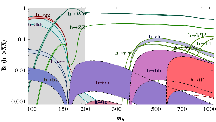
Figure 4: Decay branching fractions of the Higgs scalar in a warped scenario with four generations of fermions. The bands represent 50% likelihood for the branching ratio, according to our numerical scan, as explained in the text. The gray region below $200$ GeV is excluded by both Tevatron and LHC. The flavor anarchy setup (masses and mixings explained through fermion localization, with random 5D Yukawa couplings) predicts generic FV couplings of the Higgs, leading to a few new interesting decay channels such as $h\to bb^{\prime}$ and $h\to\tau\tau^{\prime}$. The masses chosen for this plot are $m_{b^{\prime}}=350$ GeV, $m_{t^{\prime}}=400$ GeV, $m_{\tau^{\prime}}=160$ GeV and $m_{N_{4}}=250$ GeV ($N_{4}\equiv\nu_{\tau}^{\prime}$), and the KK scale is $(R^{\prime})^{-1}=1500$ GeV.

The new and very interesting result is the prediction of sizable branching fractions for exotic decays of the Higgs into fermion pairs of different flavor. In particular we observe that $h\to\tau\tau^{\prime}$, $h\to bb^{\prime}$ and $h\to tt^{\prime}$ are among the most important new flavor violating channels, a fact not surprising since for heavier fermions one expects larger couplings to the Higgs. An interesting remark for these new channels is that the threshold mass at which they become kinematically allowed is basically set by the mass of the heaviest fermion. This means that while some or most of the flavor diagonal decays into fermions might be closed, there are good chances of an open channel such as $h\to\tau\tau^{\prime}$ or $h\to bb^{\prime}$. For the chosen parameters (KK scale of $1/R^{\prime}=1500$ GeV and typical 5D Yukawa couplings of ${\cal O}(2)$) we obtain generic flavor violating Higgs couplings which place the branching ratios of these exotic decay modes on the order of $10^{-2}$. Note that since the flavor violating couplings scale as $(\bar{Y}R^{\prime})^{2}$, the branching ratios should in turn scale as $(\bar{Y}R^{\prime})^{4}$, showing great sensitivity to both the 5D Yukawa couplings and the KK scale.

The production cross section at the LHC of a heavy Higgs of  $200-400$ GeV, in a scenario with fourth generation quarks is expected to be about  $50-70$ pb particledata . Since the new exotic decays have branching ratios at the percent level, one expects the cross section of these modes to be somewhere near $500$ fb. This means that with 1 or 2 fb^-1 of integrated luminosity at the LHC (early stages) one could have at least a few hundred of these events. Of course given the large production cross section, there would be no problem in quickly discovering the Higgs via the four lepton mode ($h\to Z^{0}Z^{0}\to 4l$) or maybe through ($h\to W^{\pm}W^{\mp}$). With the Higgs mass properly set, a complementary search for some of the new exotic channels should be much easier.

Of particular interest is the mode $h\to\tau\tau^{\prime}$ since it may actually compete as the main production mechanism for the fourth generation charged lepton. If $m_{h}<2m_{\tau^{\prime}}$, the decay into pairs of $\tau^{\prime}$ is forbidden and so the other possible production for heavy leptons is through s-channel processes involving electroweak bosons Carpenter:2010bs and their KK partners Burdman:2009ih . The typical cross section for $\tau^{\prime}-\nu_{\tau}^{\prime}$ production via $s$-channel $W$ is  $10-100$ fb Carpenter:2010bs , which means that the flavor violating production through $s$-channel on-shell Higgs of $\tau^{\pm}{\tau^{\prime}}^{\mp}$ can be a few times larger than this. The subsequent decay of the ${\tau^{\prime}}^{\mp}\to\nu_{\tau}^{\prime}W^{\mp}$, and then of $\nu_{\tau}^{\prime}\to Wl$ should give a signal of $pp\to h\to\tau^{\pm}{\tau^{\prime}}^{\mp}\to\tau^{\pm}W^{\mp}Wl$, where all particles are produced and decayed on-shell. The signs of the second $W$ and the charged lepton $l$ is not fixed and depends on the nature of $\nu_{\tau}^{\prime}$. One would look for same sign dilepton events coming from leptonic decays of the first $W$ along with the last lepton of the chain. This type of signature is quite clean thanks to the minimal background and would in principle allow for easy confirmation of the signal, which could become the discovery signal for the $\tau^{\prime}$ along with the confirmation of Higgs flavor violating couplings.

Another interesting decay mode, if kinematically allowed is $h\to bb^{\prime}$, where the $b^{\prime}$ would subsequently decay as $b^{\prime}\to q\,W$ or $b^{\prime}\to b\,Z^{0}$. In the first possibility, $q$ stands for $t$ if kinematically allowed, and for $c$ or $u$. The partial width of these channels depend on the size of the CKM4 angles $V_{tb^{\prime}}$, $V_{cb^{\prime}}$ and $V_{ub^{\prime}}$ which are typically constrained to be small Alok:2010zj . A channel which could compete is $b^{\prime}\to b\,Z^{0}$, since in the RS scenario under study these flavor violating couplings appear at tree-level, in a similar fashion as in the Higgs sector agashe ; Casagrande:2008hr . Thus depending on the decay branching ratios of the $b^{\prime}$ heavy quark (see next section) the events could be $pp\to h\to bb^{\prime}\to bW^{-}t\to bbW^{\pm}W^{\mp}\ \$ or $\ \ pp\to h\to bb^{\prime}\to bW^{-}j\ \$ or $\ \ pp\to h\to bb^{\prime}\to bbZ^{0}$. A careful study of these signals and their background is beyond the scope of this work, but we should mention that a clear prediction of our scenario is that the $h-b-b^{\prime}$ coupling is highly asymmetric (see Eq. (61)) with a definite preference for $h\to b^{\prime}_{R}b_{L}$ decay over the $h\to b^{\prime}_{L}b_{R}$. Thus one should also look for the angular correlations in the signals in order to search for this asymmetric property of the couplings (see refs. Krohn:2011tw for studies along these lines).

IV.1.4 Heavy fermion decays

• Heavy quark decays

If the Higgs masses are lighter than the masses of the fourth generation fermions, channels in which the heavy fermions decay to the Higgs boson and a fermion from one of the lighter families are open. Pair production of heavy quark flavors is expected to have a cross section of $\sim 4-4.5$ pb for a mass of $500$ GeV at the LHC with $\sqrt{s}=14$ TeV Cacciari:2008zb , thus should be within reach, and their properties would then become apparent. As the FCNC couplings of the Higgs to the fermions are proportional to fermion masses, the dominant decays would be to the third generation fermions. The flavor violating couplings of Higgs will lead to tree-level decays $t^{\prime}\rightarrow th$ and $b^{\prime}\rightarrow bh$ in the kinematically allowed regions $m_{t^{\prime}}>m_{h}+m_{t}$ and $m_{b^{\prime}}>m_{h}+m_{b}$. The decay rates for these processes are calculated as

$$\Gamma(Q_{j}\rightarrow q_{i}h) = \frac{1}{16\pi m_{j}^{3}}\sqrt{m_{i}^{4}+m_{j}^{4}+m_{h}^{4}-2m_{i}^{2}m_{j}^{2}-2m_{i}^{2}m_{h}^{2}-2m_{j}^{2}m_{h}^{2}}$$ (114)

$$\times \Big{[}(\mid a_{ij}^{u(d)}\mid^{2}+\mid a_{ji}^{u(d)}\mid^{2})(m_{j}^{2}+m_{i}^{2}-m_{h}^{2})+4\Re(a_{ij}^{u(d)}a_{ji}^{u(d)})m_{i}m_{j}\Big{]}\frac{m_{i}m_{j}}{v_{4}^{2}}.\ \ \ \$$

These decays can have significant decay width, and branching ratios. By comparison, the other dominant two body decay modes are $t^{\prime}\rightarrow bW$ and $b^{\prime}\rightarrow tW$, given by Atwood:2011kc

$$\Gamma(Q_{j}\rightarrow q_{i}W) = \frac{\alpha\left|V_{ji}\right|^{2}}{16M_{W}^{2}m_{j}^{3}}\sqrt{m_{i}^{4}+m_{j}^{4}+M_{W}^{4}-2m_{i}^{2}m_{j}^{2}-2m_{i}^{2}M_{W}^{2}-2m_{j}^{2}M_{W}^{2}}$$ (115)

$$\times \bigg{(}m_{i}^{4}+m_{j}^{4}-2M_{W}^{4}-2m_{i}^{2}m_{j}^{2}+m_{j}^{2}M_{W}^{2},\bigg{)},$$

by substituting the corresponding quarks in the two body decays. The flavor-changing couplings of quarks to the $Z^{0}$ boson allow FCNC quark decays via the process $Q\to qZ^{0}$. The branching ratio is Casagrande:2008hr

$$\Gamma(Q_{j}\to q_{i}Z^{0}) = \frac{\alpha T_{3}^{2}}{8M_{Z}^{2}\cos^{2}\theta_{W}m_{j}^{3}}\bigg{(}{\sqrt{m_{i}^{4}+m_{j}^{4}+M_{Z}^{4}-2m_{i}^{2}m_{j}^{2}-2m_{i}^{2}M_{Z}^{2}-2m_{j}^{2}M_{Z}^{2}}}\bigg{)}$$ (116)

$$\times \left\{\left(m_{j}^{2}-m_{i}^{2}\right)^{2}+M_{Z}^{2}\left(m_{j}^{2}-2M_{Z}^{2}\right)\bigg{[}\left|\left(a_{L}^{u,d}\right)_{34}\right|^{2}+\left|\left(a_{R}^{u,d}\right)_{34}\right|^{2}\bigg{]}\right.$$

$$+ \left.12\,m_{i}m_{j}^{3}\,{\Re}\big{[}\left(a_{L}^{u,d}\right)_{34}^{*}\left(a_{R}^{u,d}\right)_{34}\big{]}\right\},$$

with $T_{3}$ the third quark isospin component and with the flavor-changing couplings $a_{L}^{u,d}$ and $a_{R}^{u,d}$ as defined in given as in Eq. (96). We define the total width to be the sum of the dominant two body-decays

$$\Gamma(Q_{j}\rightarrow 2X)=\Gamma(Q_{j}\rightarrow q_{i}W)+\Gamma(Q_{j}\rightarrow q_{i}h)+\Gamma(Q_{j}\rightarrow q_{i}Z^{0}).$$ (117)

Although the decays $Q_{j}\to q^{\prime}_{i}W$, $Q_{j}\to q_{i}Z$ and $Q_{j}\to q_{i}h$, $i=1,2$ should be subdominant due to CKM and Yukawa suppression, for completeness we include them in our numerical calculations and plots.

In Figure 5 we illustrate the branching ratios for the $t^{\prime}$ quark for $m_{h}=200$ GeV (still allowed by present bounds on the Higgs in the presence of four generations Higgs mass limits ) for two choices of KK mass scales, $R^{\prime-1}=1.5$ TeV and $R^{\prime-1}=3$ TeV, and for two choices of the CKM4 mixing involved here, i.e $V_{t^{\prime}b}=0.1$ and $V_{t^{\prime}b}=0.3$. The latter will affect the tree-level decay $t^{\prime}\to b\,W$, typically assumed to be the dominant decay for the usual choice $m_{t^{\prime}}-m_{b^{\prime}}\mathrel{\raise 1.29167pt\hbox{$<$\kern-7.5pt\lower 4.30554pt\hbox{$\sim$}}}50$ GeV. The characteristic bands appearing in these figures are due to the fact that the flavor violating couplings for both Higgs and $Z^{0}$ are obtained from numerical scans, performed for different values of the heavy quark masses. To visualize the generic region in parameter space that the branchings should cover, we show the interval of couplings inside which 30$\%$ of all the generated points lie, such that 35$\%$ lie below that interval and 35$\%$ lie above. This procedure will define “bands” in the figures which should be understood as the generic region predicted by flavor anarchy, containing 30$\%$ of the random points (with 35$\%$ of the points lying above the band and 35$\%$ lying below).

We compare the dominant branching ratios for tree level decays: $t^{\prime}\to b\,W$, $t^{\prime}\to t\,h$ and $t^{\prime}\to t\,Z^{0}$, and also the subdominant decays $t^{\prime}\to q^{\prime}\,W$, $t^{\prime}\to q\,Z$ and $t^{\prime}\to q\,h$ with $q^{\prime}=d,s$ and $q=c,u$. Compared to these tree-level decays, the branching of loop-induced processes such as Br$(t^{\prime}\to t\,\gamma)\simeq{\cal O}(10^{-7})$ are much smaller. In all three plots we observe the importance of the decay rate $t^{\prime}\to t\,h$, which will generically dominate for a KK scale of $1.5$ TeV and a moderate CKM4 entry $V_{t^{\prime}b}=0.1$. By increasing the KK scale or $V_{t^{\prime}b}$, the branching of $t^{\prime}\to b\,W$ is enhanced, but we observe that the decay into Higgs and $bottom$ remains well above the 20$\%$ branching in the worst case considered.

$\begin{array}[]{ccc}\includegraphics[width=158.99377pt,height=231.26378pt]{BRtp01-1500.pdf}&\includegraphics[width=158.99377pt,height=231.26378pt]{BRtp03-1500.pdf}&\includegraphics[width=158.99377pt,height=231.26378pt]{BRtp01-3000.pdf}\\ \end{array}$

Figure 5: Branching ratios for 2-body $t^{\prime}$ decays with CKM4 mixing angle $V_{t^{\prime}b}=0.1$ and KK scale $\ \ R^{\prime-1}(\equiv M_{KK})=1.5$ TeV (left panel), $V_{t^{\prime}b}=0.3,\ R^{\prime-1}=1.5$ TeV (middle panel) and $V_{t^{\prime}b}=0.1,\ R^{\prime-1}=3$ TeV (right panel). We take $V_{t^{\prime}s}=V_{t^{\prime}d}=0.01$ and $m_{h}=200$ GeV throughout. The bands represent 30% likelihood for the branching ratio, according to our numerical scan, as explained in the text.

In general one can see that the flavor violating decays of the $t^{\prime}$ are significant for all parameter values chosen, and, as long as they are kinematically allowed, they clearly dominate over the intuitive channel $t^{\prime}\to b\,W$. Of course, the effect depends on $({R^{\prime}}^{2}\bar{Y}^{2})^{2}$ and will decouple for a large enough increase of the KK scale ${R^{\prime}}^{-1}$. Therefore, which decay is dominant depends sensitively on the KK scale $R^{\prime-1}$ and also on the CKM mixing $V_{t^{\prime}b}$. In particular, for $R^{\prime-1}=1.5$ TeV and $V_{t^{\prime}b}=0.1$ (a value favored in the fits of Alok:2010zj ), the branching ratio for $t^{\prime}\to t\,h$ seems to be predicted to be dominant and about twice as large as the one for $t^{\prime}\to b\,W$ over the allowed parameter space. While for $R^{\prime-1}=3$ TeV and $V_{t^{\prime}b}=0.1$, the branching ratio for $t^{\prime}\to t\,h$ is now predicted to be about two to three times smaller than that of $t^{\prime}\to b\,W$. For the intermediate choice, $R^{\prime-1}=1.5$ TeV and $V_{t^{\prime}\,b}=0.3$ the branching ratio for $t^{\prime}\to b\,W$ overlaps with that for $t^{\prime}\to t\,h$ over a significant range of parameter space.

In all three plots, the flavor violating decay $t^{\prime}\to tZ^{0}$ is subdominant, yet non-negligible either, with possible branchings ranging from about $1\%$ to $10\%$. This channel becomes specially interesting when the decay into Higgs is kinematically forbidden, namely for $t^{\prime}$ masses below the threshold $m_{t}+m_{h}\simeq 370$ GeV, but the decay into $top$ and $Z$ is open.

We also include the suppressed decays $t^{\prime}\to q_{i}\,h,~{}t^{\prime}\to q_{i}\,Z^{0}$ and $t^{\prime}\to q_{j}\,W,~{}i,j=1,2$. The $Z^{0}$ decay width is sometimes too small and its branching ratio falls below $10^{-3}$, which is why it does not appear in the plot. We take a generic value for $V_{t^{\prime}q_{j}}=0.01$ and include FCNC coefficients $a^{u}_{4i(i4)}$, $(a^{u}_{L})_{4i(i4)}$ from our scan.

Thus the decay $t^{\prime}\to t\,h$, if kinematically allowed, is a promising channel for observing $t^{\prime}$ pair production as well as a novel Higgs pair production channel, in the subsequent decays of the heavy quarks.

It may even be possible to see simultaneously the two dominant decays if the branching ratios happen to be of similar size, giving rise to interesting pair production processes and decays:

• $pp\to t^{\prime}t^{\prime}\to tthh$ • $pp\to t^{\prime}t^{\prime}\to bbWW$

• $pp\to t^{\prime}t^{\prime}\to tbhW$

all potentially accessible and thus providing an indirect confirmation (or at least a consistency check) of the warped extra dimensional model and its parameter space. In particular, the relative importance of these signals would provide valuable hints on the size of the KK scale as well as of the CKM4 angle $V_{t^{\prime}b}$. Note also that if the KK scale is such that $R^{\prime-1}=1.5$ TeV, the lightest KK particle in the minimal scenario would have a mass of ${\cal O}(3$ TeV) and may escape detection at the LHC, while the exotic flavor violating decays (caused by the presence of KK particles) of the fourth generation quarks would still be observable.

We perform the same analysis for the decays of the $b^{\prime}$ quark as shown in Fig. 6. As before, we choose three parameter combinations for the KK scale and for the main CKM4 mixing angle involved in these decays, i.e $R^{\prime-1}=1.5$ TeV and $V_{tb^{\prime}}=0.1$, then $R^{\prime-1}=1.5$ TeV and $V_{tb^{\prime}}=0.3$, and finally $R^{\prime-1}=3$ TeV and $V_{tb^{\prime}}=0.1$. The dependence of the branching ratios of FCNC decays of the $b^{\prime}$ quark is more or less similar to the corresponding ones for the $t^{\prime}$ quark, with the decay $b^{\prime}\to b\,h$ dominating over all others for $R^{\prime-1}=1.5$ TeV and $V_{tb^{\prime}}=0.1$, while for the two other parameter choices the decay $b^{\prime}\to t\,W$ has the largest width for $m_{b^{\prime}}\geq 250$ GeV (although it overlaps with $b^{\prime}\to b\,h$ for $V_{tb^{\prime}}=0.3,\ R^{\prime-1}=1.5$ TeV).

The flavor violating decays $b^{\prime}\to b\,h$, $b^{\prime}\to b\,Z^{0}$ have a lower kinematic threshold than $t^{\prime}\to t\,h$ and therefore can happen for $b^{\prime}$ masses just above the Higgs (or $Z^{0}$) mass. But the W-mediated decays of the $b^{\prime}$ start at a larger mass threshold than in the previous CKM decays of the $t^{\prime}$, since charged current decays of $b^{\prime}$ will involve a $top$ quark and a $W$, both heavy. This means that in the low $b^{\prime}$ mass region, the FCNC decays start dominating. Of course as the mixing angle $V_{tb^{\prime}}$ is increased, the relative importance of the charged current decay grows as expected. As before, we include the CKM4 and $a^{d}_{ij}$, $(a^{d}_{L})_{ij}$ suppressed decays $b^{\prime}\to q_{i}\,h,~{}b^{\prime}\to q_{i}\,Z^{0}$ and $b^{\prime}\to q_{j}\,W,~{}i,j=1,2$, with a generic value for $V_{b^{\prime}q_{j}}=0.01$ and including the FCNC couplings $a^{d}_{4i(i4)}$, $(a^{d}_{L})_{4i(i4)}$ from our scan.

$\begin{array}[]{ccc}\includegraphics[width=158.99377pt,height=231.26378pt]{BRbp01-1500.pdf}&\includegraphics[width=158.99377pt,height=231.26378pt]{BRbp03-1500.pdf}&\includegraphics[width=158.99377pt,height=231.26378pt]{BRbp01-3000.pdf}\\ \end{array}$

Figure 6: Branching ratios for 2-body $b^{\prime}$ decays with CKM4 mixing angle $V_{tb^{\prime}}=0.1$ and KK scale $R^{\prime-1}(\equiv M_{KK})=1.5$ TeV (left panel), $V_{tb^{\prime}}=0.3,\ R^{\prime-1}=1.5$ TeV (middle panel) and $V_{tb^{\prime}}=0.1,\ R^{\prime-1}=3$ TeV (right panel). We take $V_{cb^{\prime}}=V_{ub^{\prime}}=0.01$ throughout as well as $m_{h}=200$ GeV. The bands represent 30% likelihood for the branching ratio, according to our numerical scan, as explained in the text.

Again, the $b^{\prime}\to h\,b$ decay will be very important in all the parameter points considered, being dominant for low KK scale and small CKM4 mixing angles, and then competing with the decay $b^{\prime}\to t\,W$ when KK scale or $V_{tb^{\prime}}$ are increased. The decay $b^{\prime}\to b\,Z^{0}$ is suppressed relative to the other two, but still important, with branching ratios reaching 1% -6%.

As before, we include the CKM and Yukawa suppressed decays $b^{\prime}\to q^{\prime}\,W$, $b^{\prime}\to qh$ and $b^{\prime}\to qZ$, with $q^{\prime}=u,d$ and $q=s,d$. Again, FCNC decays of $b^{\prime}$ through Higgs or $Z^{0}$ bosons would provide an indirect indication of the warped space scenario, even for large KK scales such as $R^{\prime-1}=3$ TeV. From the plots one see that it may again be possible to observe at the same time the dominant decay modes of the $b^{\prime}$ quark (since these are produced in pairs).

For a lighter $b^{\prime}$, below the threshold for $b^{\prime}\to tW$, i.e. $m_{b}^{\prime}<250$ GeV one sees that the FCNC decays into Higgs and into $Z^{0}$ might dominate over decays into $W$ and light quarks (and hence might substantially alter the current experimental bounds on the $b^{\prime}$ mass where CKM decays are assumed). In that situation it may be possible to observe a mixture of events:

• $pp\to b^{\prime}b^{\prime}\to bbhh$ • $pp\to b^{\prime}b^{\prime}\to bbZZ$ • $pp\to b^{\prime}b^{\prime}\to qWqW$

• $pp\to b^{\prime}b^{\prime}\to qWbh$ • $pp\to b^{\prime}b^{\prime}\to bZbh$ • $pp\to b^{\prime}b^{\prime}\to bZqW$

Of these, the events containing a Higgs would be the cleanest by far, since the Higgs itself should decay into $WW$ or $ZZ$ giving rise to events with many gauge bosons.

For a heavier $b^{\prime}$, it appears that two modes should dominate, namely the FCNC decays onto Higgs and the decays into a $W$ and a top quark (due to our assumption of $V_{tb^{\prime}}$ being the largest of the CKM4 mixing angles involved). The possible mixed events could now be

• $pp\to b^{\prime}b^{\prime}\to bbhh$ • $pp\to b^{\prime}b^{\prime}\to tWtW$

• $pp\to b^{\prime}b^{\prime}\to tWbh$

All events would be easy to identify at the LHC and their relative importance would provide again valuable information on the model parameters of this scenario.

• Heavy lepton decays

Once the $\tau^{\prime}$ lepton is produced at a collider, its FCNC decay will proceed in the same manner as that of the $b^{\prime}$ quark. As the mass bounds on new $\tau^{\prime}$ leptons and $\nu_{\tau}^{\prime}$ neutrinos are close, it may be that the decay $\tau^{\prime}\to W\nu_{\tau}^{\prime}$ is kinematically forbidden, and the decay of $\tau^{\prime}$ to lighter neutrinos ($\tau^{\prime}\to W\nu_{i},\ i=1,2,3$) depends on the specific model of neutrino masses and mixing and may be suppressed. Thus the FCNC decays $\tau^{\prime}\to h\tau$, and $\tau^{\prime}\to\tau Z^{0}$ could be the most dominant decays. Since we are assuming that $m_{h}+m_{\tau}<m_{\tau^{\prime}}$, the production of $\tau^{\prime}$ should happen via $s$-channel W bosons and KK partners, and therefore would typically come with associated production of $\nu^{\prime}_{\tau}$ (if the mixing to lighter neutrinos is smaller).

The subsequent FCNC decays of $\tau^{\prime}$ should be easily disentangled at the LHC as we would obtain several possible processes with many leptons, such as $pp\to\tau^{\prime}\nu_{\tau}\to\tau hWl$ for the case of $\tau^{\prime}\to\tau h$ decays. The Higgs, being heavier than $200$ GeV, should mainly decay into pairs of gauge bosons giving rise to final states of $WWWl\tau$ or $ZZWl\tau$, i.e. three gauge bosons, one light lepton and a $\tau$, a clean enough signal at hadron machine. These might give rise to same-sign dilepton events, trilepton events, and pushing it, to 6 leptons plus $\tau$ events, when every boson decays leptonically.

In the case of $\tau^{\prime}\to\tau Z^{0}$ decays, one would similarly obtain processes like $pp\to\tau^{\prime}\nu_{\tau}\to\tau ZWl$. Again one might observe same-sign dilepton events, trilepton events and when the all bosons decay leptonically one could obtain events with four leptons and a $\tau$.

As in the previous section, a realistic analysis of these signals is beyond the scope of this work, however, it seems clear that it would not be hard to disentangle them, as the branching ratios are subdominant to $\tau^{\prime}\to h\tau$, but nonetheless significant.

V Conclusions and Outlook

In this work we analyzed the effects of Higgs flavor-violating couplings in the framework of warped extra dimensions on a fourth generation of quarks and leptons. In this model, the Higgs Yukawa couplings are misaligned with the fermion mass matrices, and this effects is even more pronounced in a model with a sequential fourth fermion family, due to cumulative effects in flavor space.

We presented both an analytical evaluation and a numerical estimate of the size of the Higgs FCNC couplings in models with flavor anarchy. The only requirement is that the three-generations quark masses and mixing angles should be reproduced in the present scheme, while the fourth generations masses and mixings are allowed to be free, limited only by $V_{CKM4}$ unitarity. We briefly discussed the possibilities for the lepton sector, which is unfortunately complicated by the lack of a well-defined model of neutrino masses and mixings; as well as revisited the FCNC couplings of the $Z^{0}$ boson with a fourth generation.

After setting up the model and evaluating the Yukawa couplings, we analyzed the new effects on low energy FCNC observables. At tree level, the new off-diagonal couplings affect $K^{0}-{\bar{K}}^{0}$, $D^{0}-{\bar{D}}^{0}$ and $B_{d,s}^{0}-{\bar{B}}_{d,s}^{0}$ mixings. We use the data to set constraints on the $a_{ij}$, the most stringent bound coming from $\epsilon_{K}$ constraining the phases of the FCNC Yukawa couplings. The constraints are similar to the those obtained in the three-generations scenario toharia1 and the bounds imposed are not stringent, even if we expect the $3\times 3$ Yukawa couplings to be reduced in the four-generation model. The Yukawa FCNC couplings contribute to loop-level processes such as $b\to s\gamma$, $t\to c\gamma$, $\tau\to e,(\mu)\gamma$ and $\mu\to e\gamma$. For the quark radiative decays, the effect is negligible compared to SM values and $Wq$ diagrams. For leptons, depending on the size of the FCNC Higgs Yukawa couplings, the radiative decays might become more important and restrict the $a_{ij}^{l}$ beyond the expectation from the numerical scan, especially from the $\mu\to e\gamma$ decays, and even more as the bounds on lepton-flavor violation are expected to improve in the near future.

As the present limits on the Higgs masses are pushed higher, especially for the case of four generations, the Higgs boson decay patterns can be substantially modified from the SM and even SM4 expectations. FCNC decay channels such as $\tau\tau^{\prime}$, $bb^{\prime}$ and even $tt^{\prime}$ open for $m_{h}\mathrel{\raise 1.29167pt\hbox{$>$\kern-7.5pt\lower 4.30554pt\hbox{$\sim$}}}200$ GeV, for present bounds on four-generation masses. Both $h\to\tau\tau^{\prime}$ could prove to be fertile grounds for discovery of the fourth generation leptons, if the decay $h\to\tau^{\prime}\tau^{\prime}$ is kinematically forbidden. Similarly, the decay $h\to bb^{\prime}$ could be an important channel for $b^{\prime}$ discovery if off-diagonal fourth generation mixing angles $V_{ub^{\prime}},V_{cb^{\prime}}$ and $V_{tb^{\prime}}$ are small. The decays are important for the whole parameter space $m_{t^{\prime}}\geq 400$ GeV, $m_{b^{\prime}}\geq 200$ GeV and would provide a clear indication of the model.

If the fourth generation quarks and leptons are heavier than the Higgs boson, their decay into lighter quarks and Higgs bosons would be a promising channel for their discovery and identification. In particular, the branching ratios for $t^{\prime}\to th$ and $b^{\prime}\to bh$ compete with $t^{\prime}\to tZ^{0}$ and $b^{\prime}\to bZ^{0}$, dominate for most of the parameter space, and approach $1$ for a significant range of $V_{t^{\prime}b},\ V_{tb^{\prime}}$ and $m_{t^{\prime}},\ m_{b^{\prime}}$ parameter space. And the fourth generation lepton which can only decay through electroweak processes, may not be able to decay into $W\nu_{\tau}^{\prime}$ or $W\nu_{\tau}$ (depending on mass and mixing constraints in the leptonic sector), making $\tau^{\prime}\to\tau h$ a dominant decay mode, and competing with $\tau^{\prime}\to\tau Z^{0}$.

Thus, even if the KK scale is heavy, and KK particles cannot be seen at the LHC, residual effects due to Higgs FCNC could provide the most promising indirect signals for the warped space scenario. Our analysis shows that in a four-generation model, which is natural in this scenario, the results could be enhanced over the model with three generations and yield measurable signals at the LHC.

VI Acknowledgments

M.T. would like to thank Kaustubh Agashe, Alex Azatov and Lijun Zhu for many discussions regarding Higgs FCNC’s in this type of scenarios. M.F. is grateful to Heather Logan for comments. This work was supported in part by NSERC of Canada under SAP105354.

VII Appendix A - Loop Calculations

We present in this appendix explicit results for some of the radiative corrections addressed in the main text.

• $b\rightarrow s\gamma$

  The amplitude of $b\rightarrow s\gamma$ decay is

  $$-i\mathcal{M}=\frac{iem_{b^{\prime}}\sqrt{m_{b}m_{s}}}{48\pi^{2}v_{4}^{2}} \Big{\{} (a_{24}^{d^{*}}a_{34}^{d}P_{L}+a_{42}^{d}a_{43}^{d^{*}}P_{R})\gamma^{\mu}\Big{[}-2C_{00}+m_{b}^{2}C_{12}-m_{s}^{2}(C_{11}+C_{12}+C_{1})$$

  $$+ m_{j}^{2}C_{0}+\frac{m_{s}^{2}}{m_{s}^{2}-m_{b}^{2}}(B_{0}+B_{1})-\frac{m_{b}^{2}}{m_{s}^{2}-m_{b}^{2}}(\tilde{B}_{0}+\tilde{B}_{1})\Big{]}$$

  $$- (a_{24}^{d^{*}}a_{34}^{d}P_{R}+a_{42}^{d}a_{43}^{d^{*}}P_{L})\gamma^{\mu}m_{s}m_{b}\Big{[}C_{1}-\frac{B_{0}+B_{1}}{m_{s}^{2}-m_{b}^{2}}+\frac{\tilde{B}_{0}+\tilde{B}_{1}}{m_{s}^{2}-m_{b}^{2}}\Big{]}$$

  $$- (a_{24}^{d^{*}}a_{43}^{d^{*}}P_{L}+a_{42}^{d}a_{34}^{d}P_{R})\gamma^{\mu}m_{b}m_{b^{\prime}}\Big{[}C_{0}-\frac{B_{0}}{m_{s}^{2}-m_{b}^{2}}+\frac{\tilde{B}_{0}}{m_{s}^{2}-m_{b}^{2}}\Big{]}$$

  $$+ (a_{24}^{d^{*}}a_{43}^{d^{*}}P_{R}+a_{42}^{d}a_{34}^{d}P_{L})\gamma^{\mu}m_{s}m_{b^{\prime}}\Big{[}C_{0}+\frac{B_{0}}{m_{s}^{2}-m_{b}^{2}}-\frac{\tilde{B}_{0}}{m_{s}^{2}-m_{b}^{2}}\Big{]}\Big{\}},$$

  where $\tilde{B}_{0}$ and $\tilde{B}_{1}$ stand for two-point coefficient functions with different arguments than $B_{0}$ and $B_{1}$. The arguments of the scalar and tensor-coefficient functions appearing in the three-point integrals are $\Big{(}P_{1}^{2},P_{2}^{2},(P_{1}+P_{2})^{2},m_{b^{\prime}}^{2},m_{h}^{2},m_{b^{\prime}}^{2}\Big{)}$. The two-point integral coefficient functions $B_{0}$ and $B_{1}$ have the arguments $\Big{(}m_{s}^{2},m_{h}^{2},m_{b^{\prime}}^{2}\Big{)}$ while the arguments of $\tilde{B}_{0}$ and $\tilde{B}_{1}$ are $\Big{(}m_{b}^{2},m_{h}^{2},m_{b^{\prime}}^{2}\Big{)}$. Although $\tilde{B}$’s depend on different arguments, their numerical values are almost the same as those of the $B$’s

  The decay rate is

  $$\Gamma(b\rightarrow s\gamma)=\frac{\langle\mathcal{M}^{2}\rangle}{16\pi m_{b}^{3}}\sqrt{m_{b}^{4}+m_{s}^{4}-2m_{b}^{2}m_{s}^{2}}.$$ (119)

• $Z\to b\bar{b}$ decay

  The radiative corrections to $Z\rightarrow b\bar{b}$ vertex are

  $$\delta g^{L}(b)=\frac{m_{b}m_{b^{\prime}}}{16\pi^{2}v_{4}^{2}} \Big{\{} g_{Zb\bar{b}}^{R}\Big{[}|a_{43}^{d}|^{2}\Big{(}-2C_{00}-m_{b}^{2}(C_{11}+C_{22}+C_{1}-C_{2})+M_{Z}^{2}C_{12}\Big{)}$$ (120)

  $$+ a_{34}^{d}a_{43}^{d}m_{b}m_{b^{\prime}}(C_{1}-C_{2})\Big{]}$$

  $$+ g_{Zb\bar{b}}^{L}\Big{[}|a_{34}^{d}|^{2}\Big{(}-m_{b}^{2}(C_{2}+C_{1}-C_{0})+m_{b^{\prime}}^{2}C_{0}\Big{)}+a_{34}^{d\star}a_{43}^{d\star}m_{b}m_{b^{\prime}}(C_{2}-C_{1})$$

  $$+ |a_{43}^{d}|^{2}\Big{(}-B_{1}+(m_{b}^{2}-m_{h}^{2}+m_{b^{\prime}}^{2})B^{\prime}_{0}\Big{)}+2a_{34}^{d}a_{43}^{d}m_{b}m_{b^{\prime}}B^{\prime}_{0}\Big{]}\Big{\}},$$

  and

  $$\delta g^{R}(b)=\frac{m_{b}m_{b^{\prime}}}{16\pi^{2}v_{4}^{2}} \Big{\{} g_{Zb\bar{b}}^{L}\Big{[}|a_{34}^{d}|^{2}\Big{(}-2C_{00}-m_{b}^{2}(C_{11}+C_{22}+C_{1}-C_{2})+M_{Z}^{2}C_{12}\Big{)}$$ (121)

  $$+ a_{34}^{d\star}a_{43}^{d\star}m_{b}m_{b^{\prime}}(C_{1}-C_{2})\Big{]}$$

  $$+ g_{Zb\bar{b}}^{L}\Big{[}|a_{43}^{d}|^{2}\Big{(}-m_{b}^{2}(C_{2}+C_{1}-C_{0})+m_{b^{\prime}}^{2}C_{0}\Big{)}+a_{34}^{d}a_{43}^{d}m_{b}m_{b^{\prime}}(C_{2}-C_{1})$$

  $$+ |a_{34}^{d}|^{2}\Big{(}-B_{1}+(m_{b}^{2}-m_{h}^{2}+m_{b^{\prime}}^{2})B^{\prime}_{0}\Big{)}+2a_{34}^{d\star}a_{43}^{d\star}m_{b}m_{b^{\prime}}B^{\prime}_{0}\Big{]}\Big{\}}.$$

  The results are in good agreement with Haber:1999zh in the limit $m_{b}\rightarrow 0$ and when the intermediate particle is the $b$ rather than the $b^{\prime}$ quark. $g_{Zb\bar{b}}^{L}$ and $g_{Zb\bar{b}}^{R}$ are the tree level $Zb\bar{b}$ couplings of the SM and they are given by

  $$g_{Zb\bar{b}}^{L} = \frac{e}{\sin\theta_{W}\cos\theta_{W}}\Big{(}-\frac{1}{2}+\frac{1}{3}\sin^{2}\theta_{W}\Big{)},$$

  $$g_{Zb\bar{b}}^{R} = \frac{e}{\sin\theta_{W}\cos\theta_{W}}\Big{(}\frac{1}{3}\sin^{2}\theta_{W}\Big{)}.$$ (122)

  The arguments of the scalar and tensor-coefficient functions Hahn:1998yk appearing in the three-point and in the two-point integrals are $\Big{(}P_{1}^{2},P_{2}^{2},(P_{1}+P_{2})^{2},m_{h}^{2},m_{b^{\prime}}^{2},m_{b^{\prime}}^{2}\Big{)}$ and $\Big{(}m_{b}^{2},m_{h}^{2},m_{b^{\prime}}^{2}\Big{)}$, respectively. We note the following:

  1. The largest contribution to $g^{L}(b)$ comes from the term $\displaystyle\frac{m_{b}m_{b^{\prime}}}{16\pi^{2}v_{4}^{2}}g_{Zb\bar{b}}^{L}|a_{34}^{d}|^{2}\left[m_{b^{\prime}}^{2}C_{0}\right]\sim 4.65202\times 10^{-6}$.

  2. The largest contribution to $g^{R}(b)$ is $\displaystyle-\frac{m_{b}m_{b^{\prime}}}{16\pi^{2}v_{4}^{2}}g_{Zb\bar{b}}^{L}|a_{34}^{d}|^{2}\left[2C_{00}\right]\sim-1.4136\times 10^{-5}$.

  3. In this calculation, even if some terms include phases, they contribute as the coefficient of either $(C_{1}-C_{2})$, which is almost equal to zero, or $B^{\prime}_{0}$ which is negligible compared to the dominant terms. Thus, the phases in the Higgs Yukawa couplings $a_{ij}$ do not affect the final result.

• $Z\to\tau^{+}\tau^{-}$

  The Higgs-mediated loop contribution to the width $\Gamma(Z\to l^{+}l^{-})$ with a heavy $\tau^{\prime}$ in the loop proceeds as $Z\to b{\bar{b}}$ and induces a non-universal correction to the $\tau^{+}\tau^{-}$ decay. However, the correction due to the FCNC in the loop is very small $\left(\delta g^{L}_{Z\tau^{+}\tau^{-}},\ \delta g^{R}_{Z\tau^{+}\tau^{-}}\simeq{\cal O}(10^{-7})\right)$ for both profiles (A) and (B) in subsection III.2.4) and thus the change in width, when compared to $\displaystyle{\Gamma(\tau^{+}\tau^{-})}/{\Gamma(e^{+}e^{-})}=1.0019\pm 0.0032$ particledata , it does not set any meaningful bound on the FCNC Higgs couplings in the leptonic sector.

VIII Appendix B - Fermion Masses in RS4

First let’s define our notation. If ${\bf A}$ is an $n\times n$ matrix, then ${[\bf A]}_{ij}$ represents its $\{ij\}$ first order minor, i.e. the determinant of the $(n-1)\times(n-1)$ submatrix obtained by removing row $i$ and column $j$ to ${\bf A}$. We will also use the notation ${\bf[A]}_{ij,\alpha\beta}$ to represent the $\{ij,\alpha\beta\}$ second order minor of ${\bf A}$, i.e. the determinant of the $(n-2)\times(n-2)$ submatrix obtained by removing rows $i$ and $\alpha$, and columns $j$ and $\beta$ to the matrix ${\bf A}$.

$$M_{u} = v\ F_{Q}Y_{u}F_{u},$$ (123)

$$M_{u}M_{u}^{+} = v^{2}\ F_{Q}Y_{u}F^{2}_{u}Y^{+}_{u}F_{Q}.$$ (124)

We can always write

$$\prod_{i=1}^{i=4}m_{i}=m_{t^{\prime}}m_{t}m_{c}m_{u}=\Big{|}Det(M_{u})\Big{|}=v^{4}\ \Big{|}Det(F_{Q})Det(Y_{u})Det(F_{u})\Big{|},$$ (125)

and to lowest order in ratios of $f_{i}$’s we can write

$$\!\!\!\prod_{i=2}^{i=4}m_{i}=m_{t^{\prime}}m_{t}m_{c}=\Big{|}[M_{u}]_{{}_{11}}\Big{|}=v^{3}\ \Big{|}[F_{u}]_{{}_{11}}[Y_{u}]_{{}_{11}}[F_{Q}]_{{}_{11}}\Big{|}=v^{3}\ f_{Q_{2}}f_{Q_{3}}f_{Q_{4}}f_{u_{2}}f_{u_{3}}f_{u_{4}}\Big{|}[Y_{u}]_{{}_{11}}\Big{|},$$ (126)

and

$$\!\!\!\prod_{i=3}^{i=4}m_{i}=m_{t^{\prime}}m_{t}=\Big{|}[M_{u}]_{{}_{11,22}}\Big{|}=v^{2}\ \Big{|}[F_{u}]_{{}_{11,22}}[Y_{u}]_{{}_{11,22}}[F_{Q}]_{{}_{11,22}}\Big{|}=v^{2}\ f_{Q_{3}}f_{Q_{4}}f_{u_{3}}f_{u_{4}}\Big{|}[Y_{u}]_{{}_{11,22}}\Big{|},$$ (127)

where we have used the property ${\bf[AB]=[A][B]}$.

We can therefore obtain the leading contributions to the quark masses

$$m_{u}=\frac{m_{t^{\prime}}m_{t}m_{c}m_{u}}{m_{t^{\prime}}m_{t}m_{c}} = v\ f_{Q_{1}}f_{u_{1}}\frac{\Big{|}Det(Y_{u})\Big{|}}{\Big{|}[Y_{u}]_{{}_{11}}\Big{|}},$$ (128)

$${\rm and}\hskip 85.35826ptm_{c}=\frac{m_{t^{\prime}}m_{t}m_{c}}{m_{t^{\prime}}m_{t}} = v\ f_{Q_{2}}f_{u_{2}}\frac{\Big{|}[Y_{u}]_{{}_{11}}\Big{|}}{\Big{|}[Y_{u}]_{{}_{11,22}}\Big{|}},$$ (129)

$${\rm and}\hskip 130.88284ptm_{t^{\prime}}m_{t} = v^{2}\ f_{Q_{3}}f_{Q_{4}}f_{u_{3}}f_{u_{4}}\Big{|}[Y_{u}]_{{}_{11,22}}\Big{|}.$$ (130)

In the down sector we have

$$M_{d} = v\ F_{Q}Y_{d}F_{d},$$ (131)

$$M_{d}M_{d}^{+} = v^{2}\ F_{Q}Y_{d}F^{2}_{d}Y^{+}_{d}F_{Q}.$$ (132)

Again, we can always write

$$\prod_{i=1}^{i=4}m_{i}=m_{b^{\prime}}m_{b}m_{s}m_{d}=\Big{|}Det(M_{d})\Big{|}=v^{4}\ \Big{|}Det(F_{Q})Det(Y_{d})Det(F_{d})\Big{|}$$ (133)

and to lowest order in ratios of $f_{i}$’s we can write

$$\!\!\!\prod_{i=2}^{i=4}m_{i}=m_{b^{\prime}}m_{b}m_{s}=\Big{|}[M_{d}]_{{}_{11}}\Big{|}=v^{3}\ \Big{|}[F_{d}]_{{}_{11}}[Y_{d}]_{{}_{11}}[F_{Q}]_{{}_{11}}\Big{|}=v^{3}\ f_{Q_{2}}f_{Q_{3}}f_{Q_{4}}f_{d_{2}}f_{d_{3}}f_{d_{4}}\Big{|}[Y_{d}]_{{}_{11}}\Big{|},$$ (134)

and

$$\!\!\!\prod_{i=3}^{i=4}m_{i}=m_{b^{\prime}}m_{b}=\Big{|}[M_{d}]_{{}_{11,22}}\Big{|}=v^{2}\ \Big{|}[F_{d}]_{{}_{11,22}}[Y_{d}]_{{}_{11,22}}[F_{Q}]_{{}_{11,22}}\Big{|}=v^{2}\ f_{Q_{3}}f_{Q_{4}}f_{d_{3}}f_{d_{4}}\Big{|}[Y_{d}]_{{}_{11,22}}\Big{|}.$$ (135)

The leading contributions to the down quark masses are

$$m_{d}=\frac{m_{b^{\prime}}m_{b}m_{s}m_{d}}{m_{b^{\prime}}m_{b}m_{s}} = v\ f_{Q_{1}}f_{d_{1}}\frac{\Big{|}Det(Y_{d})\Big{|}}{\Big{|}[Y_{d}]_{{}_{11}}\Big{|}},$$ (136)

$${\rm and}\hskip 85.35826ptm_{s}=\frac{m_{b^{\prime}}m_{b}m_{s}}{m_{b^{\prime}}m_{b}} = v\ f_{Q_{2}}f_{d_{2}}\frac{\Big{|}[Y_{d}]_{{}_{11}}\Big{|}}{\Big{|}[Y_{d}]_{{}_{11,22}}\Big{|}},$$ (137)

$${\rm and}\hskip 99.58464ptm_{b^{\prime}}m_{b} = v\ f_{Q_{3}}f_{d_{3}}f_{Q_{4}}f_{d_{4}}\Big{|}[Y_{d}]_{{}_{11,22}}\Big{|}.$$ (138)

Since $f_{Q_{3}}\sim f_{Q_{4}}$ we must have that $\frac{f_{d_{3}}}{f_{d_{4}}}\sim\frac{m_{b}}{m_{b^{\prime}}}\sim 10^{-2}$.

Because of this, we can find also

$$m_{b^{\prime}}^{2}=v^{2}\ f^{2}_{d_{4}}\left(f^{2}_{Q_{4}}|Y^{d}_{44}|^{2}+f^{2}_{Q_{3}}|Y^{d}_{34}|^{2}\right).$$ (139)

References

• (1) L. Randall and R. Sundrum, Phys. Rev. Lett.  83, 3370 (1999); L. Randall and R. Sundrum, Phys. Rev. Lett.  83, 4690 (1999).
• (2) R. Sundrum, JHEP 1101, 062 (2011).
• (3) H. Davoudiasl, J.L. Hewett and T.G. Rizzo, Phys. Lett. B473 43 (2000); A. Pomarol, Phys. Lett. B486 153 (2000).
• (4) Y. Grossman, M. Neubert, Phys. Lett.  B474, 361-371 (2000); T. Gherghetta and A. Pomarol, Nucl. Phys. B586 141 (2000); S.J. Huber, Nucl. Phys. B666 269 (2003).
• (5) K. Agashe, G. Perez and A. Soni, Phys. Rev. D71 016002(2005) ; K. Agashe, G. Perez, A. Soni, Phys. Rev.  D75, 015002 (2007); K. Agashe, M. Papucci, G. Perez and D. Pirjol, hep-ph/0509117.
• (6) K. Agashe, A. Azatov and L. Zhu, arXiv:0810.1016 [hep-ph].
• (7) O. Gedalia, G. Isidori and G. Perez, arXiv:0905.3264 [hep-ph].
• (8) M. Bona et al. [ UTfit Collaboration ], PMC Phys.  A3, 6 (2009); M. Bona et al. [ UTfit Collaboration ], Phys. Lett.  B687, 61-69 (2010); A. Lenz, U. Nierste, J. Charles, S. Descotes-Genon, A. Jantsch, C. Kaufhold, H. Lacker, S. Monteil et al., Phys. Rev.  D83, 036004 (2011);
• (9) V. M. Abazov et al. [ D0 Collaboration ], [arXiv:1106.6308 [hep-ex]]. E. Lunghi, A. Soni, JHEP 0908, 051 (2009); E. Lunghi, A. Soni, Phys. Lett.  B666, 162-165 (2008).
• (10) T. Aaltonen et. al., [CDF Collaboration], arXiv:1101.0034[hep-ex]]; T. Aaltonen et al. [CDF Collaboration], Phys. Rev. Lett.  101, 202001 (2008); V. M. Abazov et al. [D0 Collaboration], Phys. Rev. Lett.  100 142002 (2008).
• (11) E. Lunghi, A. Soni, Phys. Lett.  B697, 323-328 (2011).
• (12) W. J. Marciano, G. Valencia and S. Willenbrock, Phys. Rev. D40, 1725 (1989).
• (13) B. Holdom, Phys. Rev. D 54 (1996) 721; M. Maltoni, V. A. Novikov, L. B. Okun, A. N. Rozanov and M. I. Vysotsky, Phys. Lett. B476 (2000) 107; H. J. F. He, N. Polonsky and S. f. Su, Phys. Rev. D64 (2001) 053004; V. A. Novikov, L. B. Okun, A. N. Rozanov and M. I. Vysotsky, Phys. Lett. B529 111 (2002); G. D. Kribs, T. Plehn, M. Spannowsky and T. M. P. Tait, Phys. Rev. D76 075016 (2007).
• (14) T. Yanir, JHEP 0206 044 (2002).
• (15) H. Flacher, M. Goebel, J. Haller, A. Hocker, K. Moenig and J. Stelzer, Eur. Phys. J. C60 543 (2009); V. A. Novikov, L. B. Okun, A. N. Rozanov and M. I. Vysotsky, JETP Lett. 76 127 (2002) [Pisma Zh. Eksp. Teor. Fiz. 76 158 (2002) ] ; J. M. Frere, A. N. Rozanov and M. I. Vysotsky, Phys. Atom. Nucl. 69 355 (2006).
• (16) P. Q. Hung, Phys. Rev. Lett. 80 3000 (1998).
• (17) A. Soni, [arXiv:0907.2057 [hep-ph]]; A. Soni, A. K. Alok, A. Giri, R. Mohanta and S. Nandi, Phys. Lett. B683 302 (2010); W. S. Hou, M. Nagashima and A. Soddu, Difference in Four Generation Standard Model, Phys. Rev. D76 016004 (2007); A. Arhrib and W. S. Hou, JHEP 0607 009 (2006); W. S. Hou, M. Nagashima and A. Soddu, Phys. Rev. Lett. 95 141601 (2005).
• (18) W. S. Hou, Chin. J. Phys. 47 (2009) 134; W. -S. Hou, Y. -Y. Mao, C. -H. Shen, Phys. Rev.  D82, 036005 (2010); G. Eilam, B. Melic and J. Trampetic, Phys. Rev. D80 116003 (2009).
• (19) M. S. Carena, A. Megevand, M. Quiros and C. E. M.Wagner, Nucl. Phys. B716, 319 (2005); R. Fok and G. D. Kribs, Phys. Rev. D78 075023 (2008); Y. Kikukawa, M. Kohda and J. Yasuda, Prog. Theor. Phys. 22, 402 (2009).
• (20) M. Cvetic, G. Shiu, A. M. Uranga, Nucl. Phys.  B615, 3-32 (2001); R. F. Lebed, V. E. Mayes, [arXiv:1103.4800 [hep-ph]].
• (21) P. Q. Hung, C. Xiong, Phys. Lett.  B694, 430-434 (2011); P. Q. Hung, C. Xiong, Nucl. Phys.  B847, 160-178 (2011).
• (22) A. Lister (for the CDF collaboration), presented at ICHEP 2008, [arXiv:0810.3349 [hep-ex]]; J. Conway et al., CDF public conference note CDF/PUB/TOP/PUBLIC/10110.
• (23) L. Scodellaro (for the CDF collaboration) presented at ICHEP 2010; D. Whiteson et al., CDF public conference note CDF/PUB/TOP/PUBLIC/10243.
• (24) K. Nakamura et al. (Particle Data Group), The Review of Particle Physics, J.Phys. G: Nucl. Part. Phys. 37 075021 (2010).
• (25) M. Bona et. al. [UTfit Collabroration], JHEP 03, 049 (2008).
• (26) A. K. Alok, A. Dighe, D. London, Phys. Rev.  D83, 073008 (2011); D. Das, D. London, R. Sinha, A. Soffer, Phys. Rev.  D82, 093019 (2010); O. Eberhardt, A. Lenz, J. Rohrwild, Phys. Rev.  D82, 095006 (2010).
• (27) E. De Pree, G. Marshall, M. Sher, Phys. Rev.  D80, 037301 (2009); R. C. Cotta, J. L. Hewett, A. Ismail, M. -P. Le, T. G. Rizzo, [arXiv:1105.0039 [hep-ph]].
• (28) Z. Murdock, S. Nandi, Z. Tavartkiladze, Phys. Lett.  B668, 303-307 (2008).
• (29) A. Atre, G. Azuelos, M. Carena, T. Han, E. Ozcan, J. Santiago, G. Unel, [arXiv:1102.1987 [hep-ph]].
• (30) R. C. Cotta, K. T. K. Howe, J. L. Hewett, T. G. Rizzo, [arXiv:1105.1199 [hep-ph]]; S. Litsey, M. Sher, Phys. Rev. D80, 057701 (2009); S. Dawson, P. Jaiswal, Phys. Rev. D82, 073017 (2010).
• (31) R. Fok, G. D. Kribs, Phys. Rev.  D78, 075023 (2008).
• (32) G. Burdman and L. Da Rold, JHEP 0712, 086 (2007); G. Burdman, L. Da Rold, R. D’E. Matheus, Phys. Rev.  D82, 055015 (2010).
• (33) S. Bar-Shalom, G. Eilam, A. Soni, Phys. Lett.  B688, 195-201 (2010).
• (34) H. -S. Lee, Z. Liu, A. Soni, [arXiv:1105.3490 [hep-ph]].
• (35) K. Agashe, K. Blum, S. J. Lee, G. Perez, Phys. Rev.  D81, 075012 (2010).
• (36) W. Buchmuller and D. Wyler, Nucl. Phys.  B 268, 621 (1986): F. del Aguila, M. Perez-Victoria and J. Santiago, Phys. Lett.  B 492, 98 (2000): JHEP 0009, 011 (2000); K. S. Babu and S. Nandi, Phys. Rev.  D 62, 033002 (2000); G. F. Giudice and O. Lebedev, Phys. Lett.  B 665, 79 (2008).
• (37) K. Agashe and R. Contino, Phys. Rev.  D80, 075016 (2009).
• (38) A. Azatov, M. Toharia, L. Zhu, Phys. Rev.  D80, 035016 (2009).
• (39) S. Casagrande, F. Goertz, U. Haisch, M. Neubert, T. Pfoh, JHEP 1009, 014 (2010).
• (40) A. Azatov, M. Toharia, L. Zhu, Phys. Rev.  D82, 056004 (2010).
• (41) T. Aaltonen et al. [CDF and D0 Collaboration], [[arXiv:1005.3216 [hep-ex]].
• (42) S. Chatrchyan et al. [ CMS Collaboration ], [arXiv:1102.5429 [hep-ex]].
• (43) K. Agashe, C. Csaki, C. Grojean, M. Reece, JHEP 0712, 003 (2007); R. Barbieri, A. Pomarol, R. Rattazzi, Phys. Lett.  B591, 141-149 (2004); R. Barbieri, A. Pomarol, R. Rattazzi, A. Strumia, Nucl. Phys.  B703, 127-146 (2004).
• (44) S. Casagrande, F. Goertz, U. Haisch, M. Neubert and T. Pfoh, JHEP 0810, 094 (2008).
• (45) T. P. Cheng, M. Sher, Phys. Rev.  D35, 3484 (1987).
• (46) G. Perez and L. Randall, JHEP 0901, 077 (2009); K. Agashe, T. Okui and R. Sundrum, Phys. Rev. Lett.  102, 101801 (2009);
• (47) K. Agashe, Phys. Rev.  D80, 115020 (2009).
• (48) A. J. Buras, [arXiv:hep-ph/9806471].
• (49) M. Blanke, A. J. Buras, B. Duling, S. Gori and A. Weiler, JHEP 0903, 001 (2009).
• (50) C. Csaki, Y. Grossman, P. Tanedo, Y. Tsai, Phys. Rev.  D83, 073002 (2011). [arXiv:1004.2037 [hep-ph]].
• (51) T. Hahn, PoS ACAT2010, 078 (2010). [arXiv:1006.2231 [hep-ph]].
• (52) S. Bar-Shalom, S. Nandi, A. Soni, [arXiv:1105.6095 [hep-ph]]; P. Gambino and M. Misiak, Nucl. Phys. B611, 338 (2001).
• (53) G. Eilam, J. L. Hewett, A. Soni, Phys. Rev.  D44, 1473-1484 (1991).
• (54) J. F. Gunion, [arXiv:1105.3965 [hep-ph]].
• (55) [ CDF and D0 Collaboration ], [arXiv:1007.4587 [hep- ex]]; [The ATLAS Collaboration], ATLAS-CONF-2011-052 at: http://cdsweb.cern.ch/record/1342549.
• (56) L. M. Carpenter, A. Rajaraman and D. Whiteson, arXiv:1010.1011 [hep-ph].
• (57) D. Krohn, T. Liu, J. Shelton, L. -T. Wang, [arXiv:1105.3743 [hep-ph]]; E. L. Berger, Q. -H. Cao, C. -R. Chen, H. Zhang, [arXiv:1103.3274 [hep-ph]].
• (58) M. Cacciari, S. Frixione, M. L. Mangano, P. Nason, G. Ridolfi, JHEP 0809, 127 (2008);
• (59) D. Atwood, S. K. Gupta, A. Soni, [arXiv:1104.3874 [hep-ph]].
• (60) H. E. Haber, H. E. Logan, Phys. Rev.  D62, 015011 (2000).
• (61) T. Hahn, M. Perez-Victoria, Comput. Phys. Commun.  118, 153-165 (1999).