Coherence of a qubit stored in Zeeman levels of a single optically trapped atom

Abstract

We experimentally investigate the coherence properties of a qubit stored in the Zeeman substates of the $5^{2}S_{1/2},\>F=1$ hyperfine ground level of a single optically trapped ⁸⁷Rb atom. Larmor precession of a single atomic spin-1 system is observed by preparing the atom in a defined initial spin-state and then measuring the resulting state after a programmable period of free evolution. Additionally, by performing quantum state tomography, maximum knowledge about the spin coherence is gathered. By using an active magnetic field stabilization and without application of a magnetic guiding field we achieve transverse and longitudinal dephasing times of $T_{2}^{*}=75..150\,\mathrm{\mu s}$ and $T_{1}>0.5\,\mathrm{ms}$ respectively. We derive the light-shift distribution of a single atom in the approximately harmonic potential of a dipole trap and show that the measured atomic spin coherence is limited mainly by residual position- and state-dependent effects in the optical trapping potential. The improved understanding enables longer coherence times, an important prerequisite for future applications in long-distance quantum communication and computation with atoms in optical lattices or for a loophole-free test of Bell’s inequality.

I Introduction

Quantum memories for the storage and retrieval of quantum information play an outstanding role in future applications of quantum communication, such as quantum networks and the quantum repeater Briegel98 . There, ground states of trapped atoms or ions, are ideal candidates, as the interaction with the environment is weak and can be controlled with high accuracy. Although in such systems coherence times of the order of several seconds have been observed Davidson95 ; Kuhr05 ; Ozeri05 , storage and retrieval of single quantum excitations was shown to reach maximum times of only few $100\,\mathrm{\mu s}$ to $\mathrm{ms}$ Choi08 ; Rosenfeld08 ; Zhao09 ; Dudin09 ; Specht11 , in which storage of a complete polarization qubit state represents a greater challenge. In order to further prolong the quantum storage time a detailed understanding of dephasing and decoherence processes is indispensable.

Optical dipole traps Grimm00 nowadays are a well-established tool for the controlled manipulation of internal and external quantum states of neutral atoms Kuhr05 ; Nelson07 ; Bloch08 ; Rosenfeld08 ; Dudin09 ; Foerster09 ; Bakr09 ; Wilk10 ; Isenhower10 . Such traps provide almost ideal conservative trapping potentials combined with low heating rates, resulting in long atomic coherence times. However, two kind of effects significantly limit the achievable coherence time: (i) Off-resonant spontaneous Raman scattering from the dipole laser beam entangles the qubit of freedom with some degree of freedom of a single scattered photon Blinov04 ; Matsukevich05 ; APE06 . This kind of light-matter interaction leads to decoherence in the most general sense as the system under investigation (atomic memory qubit) gets entangled with the environment (scattered photon). (ii) In addition, if the trapped atom is not in the vibrational ground state, the thermal motion together with residual state-dependent effects of the optical trapping potential will lead to dephasing of an initial atomic spin state. Although the temporal spin-evolution in an individual experimental realization is strictly coherent, the observed ensemble average over many experimental runs may have a large scatter due to different initial conditions.

In our experiment quantum information is stored in the Zeeman sublevels of the $5^{2}S_{1/2},\>F=1$ hyperfine ground level of a single ⁸⁷Rb atom, localized in an optical dipole trap Weber06 . For a variety of applications in long-distance quantum communication, e.g., the generation of long-distance atom-photon APE06 ; Rosenfeld08 and atom-atom entanglement, as well as the closely related task of the remote preparation of an atomic quantum memory Rosenfeld07 , only a spin-1/2 subspace of the $5^{2}S_{1/2},\>F=1$ hyperfine ground level is addressed. More precisely, the atomic memory qubit is encoded in the $\left|F=1,\,m_{F}=-1\right\rangle$ and $\left|F=1,\,m_{F}=+1\right\rangle$ Zeeman sublevels. The remaining third sublevel $\left|F=1,\,m_{F}=0\right\rangle$ is not directly used for qubit storage, however, the coherent evolution of the total angular momentum $F=1$ in a magnetic field (Larmor-precession) can lead to its population, thereby reducing the fidelity of the stored state. In order to extract information how a stored quantum state becomes mixed and also to distinguish coherent from incoherent processes, the temporal evolution of the full spin-1 density matrix of the $5^{2}S_{1/2},\>F=1$ hyperfine ground level has to be investigated.

In this contribution we analyze decoherence and dephasing mechanisms and their relevance for the storage of quantum information in single optically trapped ⁸⁷Rb atoms. In detail, in Sec. II we develop a model accounting for state-dependent effects of the optical trapping potential. In order to achieve spin-coherence times of several $100\,\mathrm{\mu s}$ we implement an active magnetic field stabilization (see Sec. III). Applying partial quantum state tomography of the total angular momentum state $5^{2}S_{1/2},\>F=1$ we then investigate in detail dephasing and decoherence mechanisms. Finally, in Sec. IV we summarize our major findings and give an outlook how longer spin coherence times could be reached.

II Theoretical analysis of decoherence and dephasing mechanisms

II.1 Decoherence due to spontaneous Raman scattering

The most influential scattering process occurs due to interaction of the atom with the light of the dipole trap. In our case the dipole trap is generated by a single, sharply focused laser beam at a wavelength of $\lambda=856\,\mathrm{nm}$. Despite of the large detuning to the first dipole allowed transitions $5^{2}S_{1/2}\rightarrow 5^{2}P_{1/2}$ ($\lambda=795\,\mathrm{nm}$) and $5^{2}S_{1/2}\rightarrow 5^{2}P_{3/2}$ ($\lambda=780\,\mathrm{nm}$) in ⁸⁷Rb, there is still a finite probability to spontaneously scatter light from the dipole laser beam. This scattering process consists of two important parts. Elastic (Rayleigh) scattering occurs when the atom returns to the same state after emission of a photon. In our case this happens at a rate of $17.7\,\mathrm{Hz}$ Rosenfeld08_PhD . When the final and initial states are different, even though the states might be degenerate in energy, this process is called spontaneous Raman scattering. As demonstrated previously Blinov04 ; APE06 ; Matsukevich05 , it is this scattering process which entangles, e.g., the polarization and/or the frequency of a single scattered photon with the internal spin state of one or many atoms. Obviously, only spontaneous Raman scattering will lead to spin relaxation. Far from the atomic resonances $5^{2}S_{1/2}\rightarrow 5^{2}P_{1/2}$ and $5^{2}S_{1/2}\rightarrow 5^{2}P_{3/2}$ spontaneous Raman scattering is strongly suppressed due to destructive interference of amplitudes in the different excitation and decay channels Cline94 . Its rate is given by

$$\Gamma_{incoh}=\frac{3c^{2}\omega^{3}}{4\hbar}\left(\frac{\Gamma_{D}}{\omega_{D}^{3}}\right)^{2}\left|\frac{1}{\Delta_{D1}}-\frac{1}{\Delta_{D2}}\right|^{2}\cdot I,$$ (1)

where $\omega$ is the angular frequency of the dipole laser, $I$ its intensity, $\Delta_{D1}$ and $\Delta_{D2}$ its detuning with respect to transitions to $5^{2}P_{1/2}$ and $5^{2}P_{3/2}$ levels, $\Gamma_{D}$ is the total resonant scatter rate of the respective $D1$ and $D2$ transition, and $\omega_{D}$ the angular frequency of the corresponding atomic resonance. The rate for spontaneous Raman scattering via higher-lying $n^{2}P_{1/2}$ and $n^{2}P_{3/2}$ levels ($n>5$) is negligible due to the large detuning of the dipole laser. For our typical dipole trap parameters ($\lambda=856\,\mathrm{nm}$, $I=1.56\cdot 10^{9}\,\mathrm{W/m^{2}}$) the incoherent scatter rate is $0.11\,\mathrm{Hz}$. Thus, the atomic spin will relax on a time scale of about $10\,\mathrm{s}$, which is comparable to the lifetime of captured atoms in the trap Weber06 . We conclude that in for our experiments spin relaxation due to spontaneous Raman scattering does not limit the coherence time.

II.2 Dephasing of the atomic spin

In contrast to the possibility that the atomic spin decoheres due to entanglement with the environment, the coherent interaction with fluctuating external magnetic fields $\vec{B}$ leads to dephasing of stored quantum information. Additional spin-dephasing for trapped atoms can also be caused by the thermal motion of the atom in a state-dependent trapping potential (see Sec. II.2.3).

The optical dipole trap is based on a spatially varying, light-induced energy shift of the atomic ground levels. Assuming that all relevant detunings are larger than the hyperfine ground state splitting we obtain the light-shift for the Zeeman sublevels $\left|F=1,\,m_{F}\right\rangle$ of the $5^{2}S_{1/2}$ ground level of (see e.g. Grimm00 )

$$\Delta E_{d}=-\frac{\pi c^{2}}{2}\frac{\Gamma_{D}}{\omega_{D}^{3}}\left(\frac{1-\mathcal{P}g_{F}m_{F}}{\Delta_{D1}}+\frac{2+\mathcal{P}g_{F}m_{F}}{\Delta_{D2}}\right)I.$$ (2)

For linear polarization of the trap light ($\mathcal{P}=0$) this energy shift is equal for all magnetic sublevels $m_{F}$ of both hyperfine ground levels $5^{2}S_{1/2},F=1$ and $5^{2}S_{1/2},F=2$ and therefore ideally suited as a state-insensitive trapping potential. However, in the case of circular polarization ($\mathcal{P}=+1$ for $\sigma^{+}$ and $\mathcal{P}=-1$ for $\sigma^{-}$) the shift becomes state-dependent, lifting the degeneracy of the Zeeman sublevels. This additional effect on the magnetic sublevels $m_{F}\neq 0$ for circularly polarized light is formally equivalent to a magnetic field $B_{\sigma}$ pointing along the propagation direction $z$ of the dipole laser beam, and is called vector light shift (also Zeeman light shift) vectorLightShift . In contrast to an external magnetic field which can be considered homogeneous over the microscopic volume of the optical dipole trap, the vector light shift depends on the intensity and thus on the position of the atom in the trap. For a typical temperature of the atom of $100..150\,\mathrm{\mu K}$ the thermal motion will lead to a non-negligible variation of light shifts, which significantly influence the dephasing of stored quantum information. This dephasing mechanism will be analyzed in the following.

II.2.1 Coherent state evolution

As a first step we calculate the coherent temporal evolution of the spin-1 state $|\Psi(t)\rangle$ in a constant effective magnetic field $B_{eff}$. The interaction Hamiltonian $\hat{H}_{eff}$ is given by

$$\hat{H}_{eff}=\vec{B}_{eff}\cdot\frac{\mu_{B}g_{F}}{\hbar}\hat{\vec{F}},$$ (3)

where $\hat{\vec{F}}$ is the operator of the corresponding angular momentum $F=1$, $\mu_{B}=\hbar\cdot 2\pi\cdot 1.4\,\mathrm{MHz/G}$ is the Bohr magneton and $g_{F}=-1/2$ the Landé factor. The effective magnetic field $\vec{B}_{eff}$ is given by

$$\vec{B}_{eff}=\vec{B}+B_{\sigma}\cdot\vec{\mathrm{e}}_{z}=\vec{B}+\mathcal{P}\frac{1}{\mu_{B}}\frac{\pi c^{2}}{2}\frac{\Gamma_{D}}{\omega_{D}^{3}}\left(\frac{1}{\Delta_{D1}}-\frac{1}{\Delta_{D2}}\right)I_{\sigma}\cdot\vec{\mathrm{e}}_{z},$$ (4)

with $I_{\sigma}$ the intensity of the circularly polarized component of the dipole trap beam. For convenience we set $\vec{B}_{eff}=B_{eff}(b_{x}\vec{\mathrm{e}}_{x}+b_{y}\vec{\mathrm{e}}_{y}+b_{z}\vec{\mathrm{e}}_{z})$, where $b_{x}=\sqrt{1-b_{z}^{2}}\cos(\phi)$, $b_{y}=\sqrt{1-b_{z}^{2}}\sin(\phi)$.

For this field configuration we obtain the eigenstates $\left|\Phi_{-1}\right\rangle,\,\left|\Phi_{0}\right\rangle,\,\left|\Phi_{+1}\right\rangle$ of the interaction Hamiltonian $\hat{H}_{eff}$

$$\left|\Phi_{+1}\right\rangle= \left(\begin{array}[]{c}\frac{1}{2}(1+b_{z})e^{-i\phi}\\ \frac{1}{\sqrt{2}}\sqrt{1-b_{z}^{2}}\\ \frac{1}{2}(1-b_{z})e^{i\phi}\end{array}\right),$$ (8)

$$\left|\Phi_{0}\right\rangle= \left(\begin{array}[]{c}-\frac{1}{\sqrt{2}}\sqrt{1-b_{z}^{2}}e^{-i\phi}\\ b_{z}\\ \frac{1}{\sqrt{2}}\sqrt{1-b_{z}^{2}}e^{i\phi}\end{array}\right),$$ (12)

$$\left|\Phi_{-1}\right\rangle= \left(\begin{array}[]{c}\frac{1}{2}(1-b_{z})e^{-i\phi}\\ -\frac{1}{\sqrt{2}}\sqrt{1-b_{z}^{2}}\\ \frac{1}{2}(1+b_{z})e^{i\phi}\end{array}\right),$$ (16)

with corresponding eigenvalues $+\hbar\omega_{L}$, $0$, $-\hbar\omega_{L}$, and Larmor frequency $\omega_{L}=\frac{1}{\hbar}\mu_{B}g_{F}B_{eff}$. These are $m_{F}=+1,0,-1$ eigenstates with respect to the direction of the effective magnetic field. Finally, for the time evolution of an arbitrary $5^{2}S_{1/2},\,F=1$ state we obtain

$$\left|\Psi(t)\right\rangle=c_{-1}\left|\Phi_{-1}\right\rangle e^{i\omega_{L}t}+c_{0}\left|\Phi_{0}\right\rangle+c_{+1}\left|\Phi_{+1}\right\rangle e^{-i\omega_{L}t},$$ (17)

where the amplitudes are given by $c_{\pm 1}=\left\langle\Phi_{\pm 1}|\Psi(t=0)\right\rangle$, $c_{0}=\left\langle\Phi_{0}|\Psi(t=0)\right\rangle$. Obviously, the Larmor precession in an effective magnetic field $\vec{B}_{eff}$ is thus not necessarily limited to the qubit space $\{\left|1,-1\rangle,\right|1,+1\rangle\}$.

II.2.2 Fluctuations of the magnetic fields

As a first step in the analysis of dephasing mechanisms one has to know the magnitude of magnetic field fluctuations at the relevant time scales. Typically, our experiments require preservation of the atomic quantum state for several microseconds remark01 . In this work we consider times up to $200\,\mathrm{\mu s}$, defining two important frequency ranges. The first range contains frequencies, where the magnetic field varies rapidly on the experimental time scale ($\Omega>2\pi\cdot 2.5\,\mathrm{kHz}$). In the second range we have $\Omega<2\pi\cdot 2.5\,\mathrm{kHz}$, i.e., the field can be considered constant within one experimental run, but will vary between different runs. With the help of a magneto-resistive sensor (accessible frequency range: $\mathrm{DC}-60\,\mathrm{kHz}$) we were able to quantify the magnitude of magnetic fields at different frequencies, see Sec. III.2. We found that the strongest fluctuations were at low frequencies ($<200\,\mathrm{Hz}$) while faster fluctuations were relatively small ($<0.3\,\mathrm{mG}$ rms within the bandwidth of $60\,\mathrm{kHz}$). Magnetic field fluctuations at different frequencies affect the atomic state in different ways as will be discussed below.

In the case where the field fluctuates rapidly on the experimental time scale (and also rapidly compared to the Larmor frequency $\omega_{L}$), the evolution of the atomic state will follow the average field $\bar{B}$ with small oscillations around the main trajectory. If the average field $\bar{B}$ is constant, only those deviations will lead to dephasing. The magnitude of these deviations can be estimated by solving the time-dependent Schrödinger equation in a field modulated at a frequency $\Omega\gg\omega_{L}$ and was found to drop with increasing modulation frequency as $1/\Omega^{2}$ Rosenfeld08_PhD . This can be understood as the atomic spin, which rotates at a finite Larmor frequency, can not follow the increasing frequency of the field fluctuations which therefore average out. Thus, as the magnitude of rapid fluctuations in our experiment is small ($<0.3\,\mathrm{mG}$) and due to the additional $1/\Omega^{2}$ suppression, we conclude that the influence of rapid oscillations is negligible, particularly when compared to the effect due to the slowly varying field component.

For fluctuations of the magnetic field which are slow on the time scale of a single experimental run, the field can be considered constant and the atomic state will evolve according to Eq. (17). However, the field can vary between repeated experimental runs. This inevitably leads to different evolutions of the atomic state and therefore the observed average state populations are washed out. This dephasing can be modeled by first calculating the temporal evolution of the considered state $|\Psi\rangle$ in a constant effective magnetic field $\vec{B}_{eff}$ according to Eq. (17), and incoherently averaging over states resulting from the distribution of different magnetic fields corresponding to different experimental runs.

In our spin-precession experiments we start with an initial state $|\Psi\rangle$ and let it precess for a time $t$ giving $|\Psi\rangle(t)$. Then the population of a chosen analysis state $|\Psi_{a}\rangle$ is obtained from the overlap with the precessed state, averaged over all possible evolutions. It is given by

$$P(\Psi_{a})(t)=\\ =\int dB_{x}dB_{y}dB_{z}\left(p_{x}(B_{x})p_{y}(B_{y})p_{z}(B_{z})|\langle\Psi_{a}|\Psi\rangle(t)|^{2}\right),$$ (18)

where the $p_{j}(B_{j})$ are the normalized distributions for the $j=x,y,z$ components of the effective magnetic field. If, e.g., the average values are $\bar{B}_{x}=\bar{B}_{y}=\bar{B}_{z}=0$, and the z-component of the effective magnetic field follows a Gaussian distribution

$$p_{z}(B_{z})=\frac{1}{\sqrt{\pi}\Delta B_{z}}\exp(-(\frac{B_{z}}{\Delta B_{z}})^{2}),$$ (19)

then, after initially preparing the atomic spin state $|\psi_{1}\rangle=\frac{1}{\sqrt{2}}(|1,-1\rangle+e^{i\phi}|1,+1\rangle)$, we get for the probability to stay in this state after a time $t$

$$P(\psi_{1})(t)=\frac{1}{2}\left(1+\exp(-(\frac{t}{T_{2}^{\ast}})^{2})\right).$$ (20)

Here $T_{2}^{\ast}=\frac{\hbar}{\mu_{B}g_{F}\Delta B_{z}}$ can be associated with the transverse coherence time of two-level systems Bloembergen48 . Note that the decay for this noise model (19) is not exponential.

As a second example we consider the dephasing of the spin-states $|\psi_{2}\rangle=|1,\pm 1\rangle$ in a fluctuating magnetic field along the $x$-axis. By averaging over the Gaussian distribution $p_{x}(B_{x})$ as in (19) we find

$$P(\psi_{2})(t)=\frac{1}{8}\left(3+5\cdot\exp(-(\frac{t}{T})^{2})\right).$$ (21)

Here, the state population decays with a time constant $T=\frac{2\hbar}{\mu_{B}g_{F}\Delta B_{x}}$, which is twice as long as $T_{2}^{\ast}$. $P(\psi_{2})(t)$ approaches the limit of $\frac{3}{8}$, as the corresponding spin evolution leaves the qubit subspace $\{|1,-1\rangle,|1,+1\rangle\}$. Such a situation does not occur in two-level systems and represents a more complex dephasing scenario. For more general cases the integral in (18) is not analytic.

II.2.3 Effective fluctuation of the light shift

The second part of the effective magnetic field - the vector light shift - results from the circularly polarized component of the dipole trap light and is proportional to its intensity. Due to the thermal motion of the atom in the trap, in each realization of the experiment the atom will be found at a random position within the trapping potential and will therefore be subject to a different light shift (see inset of Fig. 1). Here we shall consider the case, where the atom can be considered static within one experimental run. In our experiment the shortest oscillation period in the trap is $44\,\mathrm{\mu s}$, therefore this assumption is strictly valid only for shorter time scales. Nevertheless, even for longer experimental times it represents a worst-case assumption, since a static field which changes from experiment to experiment leads to a stronger dephasing than a field of the same amplitude which fluctuates on the experimental time scale or faster (see Sec. II.2.2).

The distribution of positions depends on the thermal energy of the trapped atom and maps directly onto a distribution of the induced magnetic field $B_{\sigma}$. To derive this distribution one has to know the 3D distribution of the corresponding potential energy. For a thermal energy sufficiently lower than the trap depth the potential can be considered harmonic and the distribution $p(\Delta B_{\sigma})$ is calculated as follows.

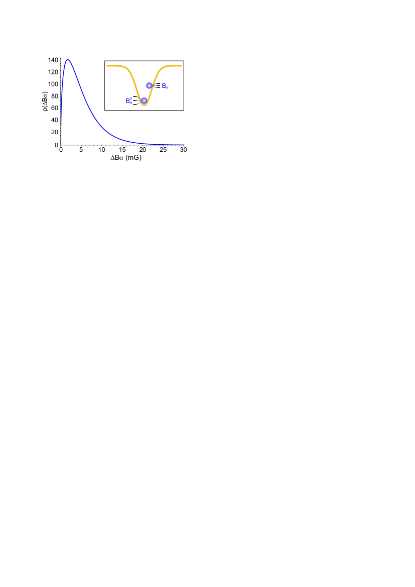
Figure 1: Probability density $p(\Delta B_{\sigma})$ of the optically induced magnetic field in a three-dimensional harmonic trap resulting from thermal motion of the atom. The distribution is plotted as a function of the deviation $\Delta B_{\sigma}=B_{\sigma}^{0}-B_{\sigma}$ of the field $B_{\sigma}$ from its maximal value $B_{\sigma}^{0}$ at the bottom of the trap. The curve was calculated according to Eq. (27), assuming a trap depth $U_{0}=k_{B}\cdot 650\,\mathrm{\mu K}$, average atomic temperature $T=150\,\mathrm{\mu K}$ and $1\%$ fraction of circularly polarized trap light.

The potential energy $U$ of a 1-dimensional harmonic oscillator can be written as

$$U(E,\varphi)=E\sin(\varphi)^{2},$$ (22)

where $E$ is the fixed total energy of the motion and $\varphi$ is the phase of the oscillation. We define the potential energy $U$ being non-negative, with $U=0$ at the bottom of the harmonic trap. If at a certain random moment of time the potential energy is measured, some random realization for the phase $\varphi\in[0..2\pi]$ will be found, where every value of $\varphi$ has equal probability. Then the probability to obtain a value of the potential energy within the interval $[U,U+dU]$ is $p_{E}(U)dU\propto d\varphi(U)$. Here, $p_{E}(U)$ is the probability density for a given total energy $E$, given by

$$p_{E}(U)=\frac{2}{\pi}\frac{d\varphi}{dU}=\frac{1}{\pi}\frac{1}{\sqrt{U(E-U)}}.$$ (23)

In thermal equilibrium the total energy $E$ follows a Boltzmann distribution. The corresponding thermal distribution of the potential energy $U$ is given by

$$p_{1D}(U)=\int_{0}^{\infty}dEp_{E}(U)\frac{1}{k_{B}T}\exp(-\frac{E}{k_{B}T})\\ =\frac{1}{\sqrt{\pi}\sqrt{k_{B}T}}\frac{1}{\sqrt{U}}\exp(-\frac{U}{k_{B}T}).$$ (24)

For three dimensions the thermal distribution of $U$ is obtained from a convolution of the three independent 1D distributions Rosenfeld08_PhD , resulting in

$$p_{3D}(U)=\frac{2}{\sqrt{\pi}(k_{B}T)^{3/2}}\sqrt{U}\exp(-\frac{U}{k_{B}T}).$$ (25)

The corresponding kinetic energy $E_{kin}$ follows the same distribution.

Here, it is worth mentioning that the distribution (25) differs from the well-known Maxwell-Boltzmann distribution, which is $p_{MB}(E)=\frac{1}{2(k_{B}T)^{3}}E^{2}\exp(-\frac{E}{k_{B}T})$. According to the Virial theorem the average of the potential energy is half of the total energy: $\left\langle U\right\rangle=\frac{1}{2}E$. This relation might suggest that the potential and kinetic energy follow the same distributions as the total energy $E$. However, that is not the case. The Virial theorem makes only a statement about average values, while the considered distribution describes the probability to find a certain value of potential energy at a randomly chosen point in time (and is therefore not ergodic). Instead, it can be easily verified that the convolution of the distribution (25) of the potential energy $U$ and of the identical distribution $p_{3D}(E_{kin})$ of the kinetic energy $E_{kin}$ gives the expected Maxwell-Boltzmann distribution of the total energy

$$\int p_{3D}(U=E-E_{kin})p_{3D}(E_{kin})dE_{kin}=p_{MB}(E).$$ (26)

Now we are able to derive the distribution $p(\Delta B_{\sigma},T)$ of the optically induced magnetic field $B_{\sigma}$ for a thermal atom at a given temperature $T$. For convenience we introduce the maximal value of the optically induced magnetic field at the bottom of the trap $B_{\sigma}^{0}$ according to Eq. (4). For our typical trap parameters $1\%$ of circular admixture in the polarization of the trapping light results in $B_{\sigma}^{0}\approx 10\,\mathrm{mG}$. The relation between the induced magnetic field and the potential energy $U$ is $B_{\sigma}(U)=B_{\sigma}^{0}\frac{U_{0}-U}{U_{0}}$. Finally, we define the deviation $\Delta B_{\sigma}=B_{\sigma}^{0}-B_{\sigma}$ from the maximal value $B_{\sigma}^{0}$ at the trap center (Fig. 1, inset). Using these relations we obtain the distribution of the optically induced magnetic field for an atom at a temperature $T$

$$p(\Delta B_{\sigma},T)=\frac{2}{\sqrt{\pi}(\frac{B_{\sigma}^{0}}{U_{0}})^{3/2}(k_{B}T)^{3/2}}\sqrt{\Delta B_{\sigma}}\exp(-\frac{\frac{U_{0}}{B_{\sigma}^{0}}\Delta B_{\sigma}}{k_{B}T}).$$ (27)

This distribution is shown in Fig. 1 for typical experimental parameters.

Expression (27) directly relates the thermal motion of the trapped atom and the circular admixture in the polarization of the trapping light to a fluctuating effective magnetic field. These fluctuations can have a serious impact on the achievable coherence times as will be shown in Sec. III.

III Experimental analysis of dephasing mechanisms

III.1 Single atom trap

In our experiment a single ⁸⁷Rb atom is stored in the optical dipole trap APE06 ; Weber06 , which is loaded from a laser-cooled cloud of $10^{3}..10^{4}$ atoms of a shallow magneto-optical trap (MOT). The conservative optical trapping potential is created by a focused Gaussian laser beam (waist $w_{0}=3.5\,\mathrm{\mu m}$; Rayleigh range $z_{R}=45\,\mathrm{\mu m}$) at a wavelength of $856\,\mathrm{nm}$, thereby detuned far to the red of any atomic transition from the atomic ground level. For a typical power of $P=30\,\mathrm{mW}$ we achieve a potential depth of $U_{0}=k_{B}\cdot 650\,\mathrm{\mu K}$, corresponding to radial and axial trap frequencies of $\omega_{r}=2\pi\cdot 22.7\,\mathrm{kHz}$ and $\omega_{z}=2\pi\cdot 1.25\,\mathrm{kHz}$, respectively. This trap provides a storage time of several seconds, mainly limited by collisions with the thermal background gas Weber06 . The fluorescence light of the trapped atom is collected in a confocal arrangement by an objective, coupled into a single mode optical fiber and guided to two single photon counting avalanche photo-detectors (APDs) allowing also a polarization analysis of single photons. The presence of a single trapped atom is inferred by detecting fluorescence light. The bare detection efficiency for a single photon emitted by the atom is $2\cdot 10^{-3}$, including coupling losses into the single-mode optical fiber and the limited quantum efficiency of the single photon detectors.

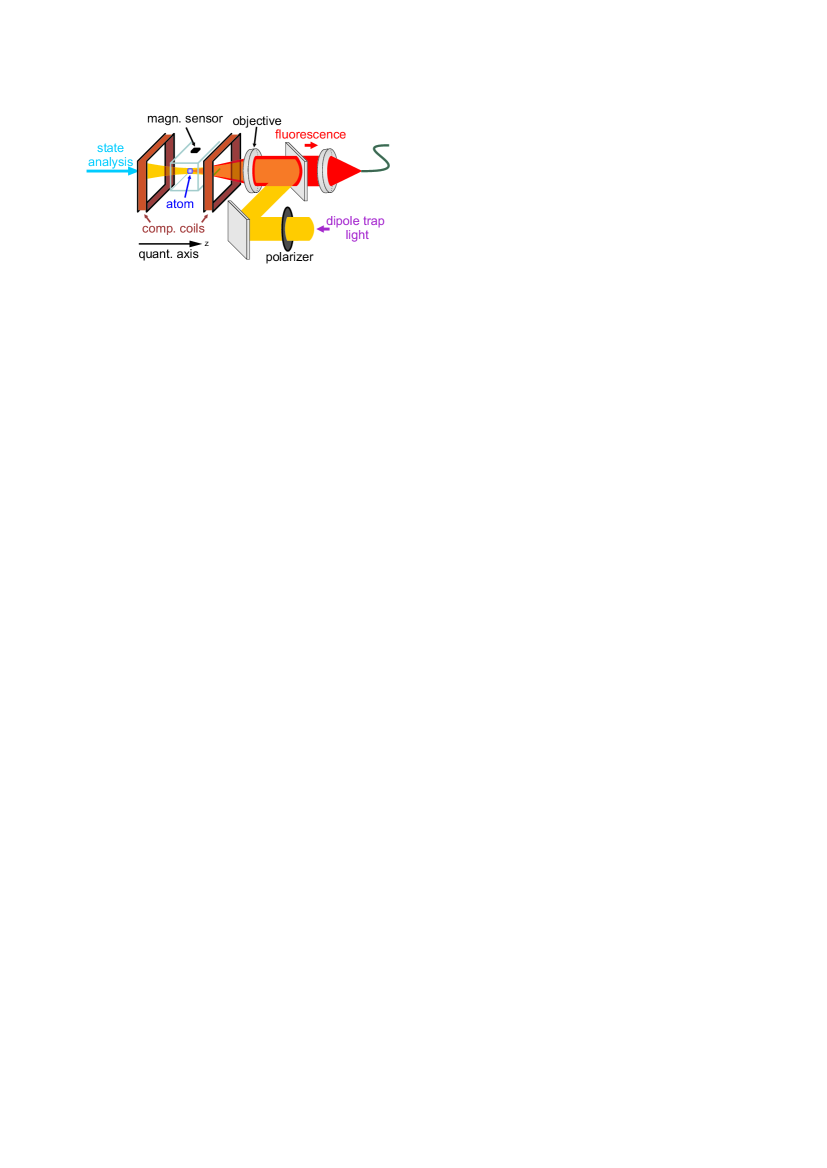
Figure 2: (Color online) Schematic of the experimental setup (not to scale). The dipole trap beam is focused into a vacuum cell by means of a high NA objective. The same objective collects the light emitted by the atom into a single mode optical fiber. The magnetic field sensor positioned on the cell surface is used to give a feedback signal to compensation coils for field stabilization. For simplicity, only one pair of compensation coils is shown.

III.2 Active magnetic field control

A crucial requirement for achieving long atomic coherence times is a precise control of the magnetic field in the region of the optical dipole trap. For this purpose the fields in our experiment are actively stabilized. The magnetic field is continuously monitored by a three-axis magneto-resistive sensor (Honeywell HMC1053), which is located outside the vacuum glass cell at a distance of $25\,\mathrm{mm}$ from the position of the trapped atom (see Fig. 2). On a short time scale the precision of this sensor is limited by electronic noise (typically $\leq 0.1\,\mathrm{mG}$ rms within the effective bandwidth of $60\,\mathrm{kHz}$). A more significant problem is saturation of the sensor by the strong fields during loading of the MOT. In this case a re-magnetization of the sensor is required which limits the precision to $0.5..1\,\mathrm{mG}$ on long time scales. Using this sensor we have measured the fluctuations of the magnetic fields and could identify two main sources. The largest part of the fluctuations is due to currents drawn by the Munich underground train line passing at a distance of about $60\,\mathrm{m}$ from our laboratory. The time scale of these fluctuations is $30\,\mathrm{s}..1\,\mathrm{min}$ with a peak-to-peak amplitude of $20..25\,\mathrm{mG}$ on the vertical and $6..8\,\mathrm{mG}$ on the horizontal axis. The second major contribution arises from the $50\,\mathrm{Hz}$ mains supply producing fluctuations of about $1..2\,\mathrm{mG}$ peak to peak on each axis. For frequencies higher than the fourth harmonic of the power line frequency ($200\,\mathrm{Hz}$) the fluctuations were found to be on the order of $\leq 0.3\,\mathrm{mG}$ rms.

The signal from the magnetic field sensor is fed back to compensation coils by means of a servo loop. The integration time constant was set such that an active bandwidth of about $200\,\mathrm{Hz}$ was reached, sufficient to suppress the effects of underground trains and the power supply line. Given the fluctuations of external fields described above, our active magnetic field stabilization achieves an rms stability of $(0.92,\,0.77,\,0.83)\,\mathrm{mG}$ for the three axes, including re-magnetization precision of the sensor, crosstalk between different axes $(\leq 3.5\%)$ and magnetic field gradients between the position of the trapped atom and the position of the sensor $(\leq 5\%)$.

III.3 State preparation and detection

To study dephasing of a single atomic spin $5^{2}S_{1/2},\,F=1$ we initialize the atom with high fidelity in a well-defined state of our choice. This is realized by first entangling the atomic Zeeman-states $|F=1,m_{F}=-1\rangle$ and $|F=1,m_{F}=+1\rangle$ with the polarization states $|\sigma^{+}\rangle$ and $|\sigma^{-}\rangle$ of a single emitted photon APE06 ; Rosenfeld07 ; Rosenfeld08 - the entangled state reads $\left|\Psi^{+}\right\rangle=\frac{1}{\sqrt{2}}(\left|1,-1\right\rangle\left|\sigma^{+}\right\rangle+\left|1,+1\right\rangle\left|\sigma^{-}\right\rangle)$ - and then projecting the atom onto the desired spin-state via a polarization measurement of the photon. Thus, a measurement of the photon in, e.g., the $\sigma^{\pm}$-basis (circularly polarized) leaves the atom in the $\left|1,\mp 1\right\rangle$ state and a measurement in $H/V$-basis (horizontally/vertically polarized) projects the atom into the $\frac{1}{\sqrt{2}}(\left|1,-1\right\rangle\pm\left|1,+1\right\rangle)$ states, respectively.

After preparation, the atomic spin freely evolves for a defined period of time in the applied magnetic field $B$. During this time all lasers except for the one used for the dipole trap are switched off and the magnetic field is stabilized to a preselected value. Finally, after a given time, the atomic state detection procedure APE06 is applied, allowing us to determine the projection of the atomic state on any superposition in the $\{\left|1,-1\right\rangle,\left|1,+1\right\rangle\}$ subspace. By these means we can directly observe the temporal evolution of selected atomic states (see Fig. 3).

III.4 Analysis of the state evolution

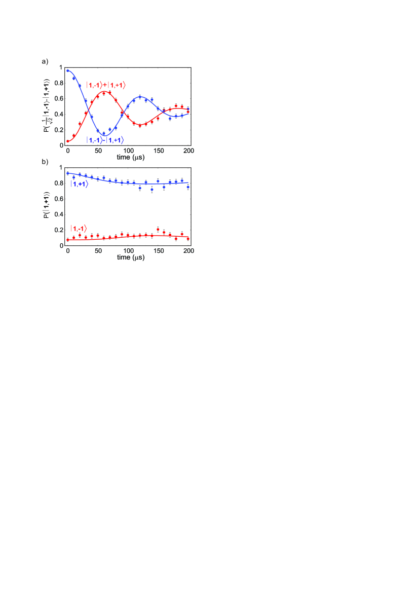
Figure 3: (Color online) Temporal evolution of different atomic spin states. a) Evolution of the superposition states $\frac{1}{\sqrt{2}}(\left|1,-1\right\rangle\pm\left|1,+1\right\rangle)$ in an effective magnetic field of $5.5\,\mathrm{mG}$ along the quantization axis. b) Evolution of states $\left|1,\pm 1\right\rangle$ in a field compensated to $B\leq 2\,\mathrm{mG}$. Measured were the populations of the spin states $\frac{1}{\sqrt{2}}(\left|1,-1\right\rangle-\left|1,+1\right\rangle)$ in a) and $\left|1,+1\right\rangle$ in b), respectively. The solid lines represent numerical fits of the measured data to the dephasing model in Eq. (18), which mainly incorporates fluctuations of the effective magnetic field due to the vector light shift.

In a first measurement, the spin states $\frac{1}{\sqrt{2}}(\left|1,-1\right\rangle\pm\left|1,+1\right\rangle)$ were prepared and a small guiding field of $5.5\,\mathrm{mG}$ was applied along the quantization axis $z$ such that a slow oscillation ($\sim 8\,\mathrm{kHz}$) could be observed. The remaining field components $B_{x}$ and $B_{y}$ were compensated below $1\,\mathrm{mG}$. After the prepared spin-states evolved a programmable period of time, the population of the $\frac{1}{\sqrt{2}}(\left|1,-1\right\rangle-\left|1,+1\right\rangle)$ state was measured, see Fig. 3 (a). For such a field configuration, where $B_{z}$ dominates all other fields, the atomic state will stay within the subspace $\{\left|1,-1\right\rangle,\left|1,+1\right\rangle\}$ during the Larmor precession, as $\left|1,\pm 1\right\rangle$ are eigenstates of the interaction Hamiltonian. We observe the expected precession of an effective spin-1/2 system with a $1/e$ dephasing time of about $120\,\mathrm{\mu s}$. In order to extract the parameters responsible for the dephasing we have numerically fitted the dephasing model from Eq. (18) to the data points in Fig. 3 (a). This model includes fluctuations of the effective magnetic field consisting of residual fluctuations of external magnetic fields along the $x$-axis (uniformly distributed) and the dominating distribution $p(\Delta B_{\sigma},T)$ of the optically induced effective field (27). For the fit we assumed a trap depth of $U_{0}=650\,\mathrm{\mu K}$ and an average atomic temperature of $150\,\mathrm{\mu K}$. The Larmor frequency deduced from this measurement corresponds to an average effective magnetic field component of $\bar{B}_{z}=(5.5\pm 0.5)\,\mathrm{mG}$ composed of the optically induced field and the externally applied magnetic field. The observed dephasing is compatible with a standard deviation of the field distribution of $2.25\,\mathrm{mG}$ along the quantization axis. From this value we deduce a fraction of $0.6\%$ of circularly polarized trapping light. This non-negligible fraction is due to the birefringence of the UHV glass cell where the experiment is performed. The birefringence is induced by mechanical stress and is not uniform over the walls of the cell, limiting the degree of control of light polarization at the position of the atomic trap.

In a second measurement the evolution of the spin states $\left|1,\pm 1\right\rangle$ was investigated. Here the absolute value of the effective magnetic field was compensated to $B\leq 2\,\mathrm{mG}$. According to Fig. 3(b), the stability of these states largely exceeds those of superpositions. This can be easily understood since the states $\left|1,\pm 1\right\rangle$ are eigenstates of the effective magnetic field pointing along the quantization axis $z$, and therefore are not affected by the fluctuations along this axis. The slower dephasing of the states $\left|1,\pm 1\right\rangle$ shows that fluctuations along the $x$ and $y$ axes are smaller than along $z$.

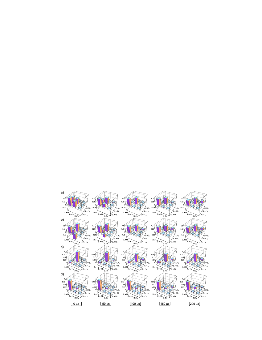
Figure 4: (Color online) Partial tomographic reconstruction of the quantum state evolution. Shown are the density matrices (real part) for the prepared states $\frac{1}{\sqrt{2}}(\left|1,-1\right\rangle\pm\left|1,+1\right\rangle)$ in a) and b), and $\left|1,\mp 1\right\rangle$ in c) and d).

III.5 Quantum state tomography

The measurement of the temporal evolution of the atomic state provides a good way to determine its coherence properties. However, state analysis in one basis does not give complete information about the qubit state under study. As the ground state $5^{2}S_{1/2},F=1$ of ⁸⁷Rb has total angular momentum of one, the respective temporal evolution involves three Zeeman sublevels: $m_{F}=\pm 1$ and $m_{F}=0$. Thus the analysis of dephasing processes becomes even more complex compared to a simple qubit state.

The best way is a complete quantum state tomography (e.g. quantumTomography and references therein), allowing to extract the information on how the state becomes mixed and also to distinguish coherent and incoherent processes. Unfortunately, a complete tomography of the spin-1 space in general requires 5 Stern-Gerlach-like measurements (each providing the populations of the 3 spin-1 eigenstates along a certain direction) spinTomography which are not accessible in our experiment. In particular, the coherences between the $\left|1,\pm 1\right\rangle$ Zeeman states and the $\left|1,0\right\rangle$ state can not be measured with our current technique, as the applied stimulated Raman adiabatic passage pulses analyze only the effective spin-1/2 subspace $\{\left|1,-1\right\rangle,\left|1,+1\right\rangle\}$ in a complete way APE06 ; Rosenfeld07 . However, as the detection efficiency is close to unity, we can infer the population $\rho_{00}$ of the $|1,0\rangle$ state as the population missing in the $\{\left|1,-1\right\rangle,\left|1,+1\right\rangle\}$ subspace.

To reconstruct the density matrix $\rho$ of the spin-1 ground state $5^{2}S_{1/2},F=1$, we use the worst-case assumption that there is no coherence between the $|1,0\rangle$ state and the $\left|1,\pm 1\right\rangle$ states. We therefore set the corresponding off-diagonal density matrix elements to zero. The corresponding full $3\times 3$ spin-1 density matrix is then given by

$$\rho=\left(\begin{array}[]{cc}\rho_{s}&\begin{array}[]{c}0\\ 0\end{array}\\ \begin{array}[]{cc}0&0\end{array}&\rho_{00}\end{array}\right).$$ (28)

Here $\rho_{s}$ is the $2\times 2$ density matrix of the spin-1/2 subspace $\{\left|1,-1\right\rangle,\left|1,+1\right\rangle\}$ and $\rho_{00}=1-trace(\rho_{s})$. As we typically measure populations of the states $\left|1,\pm 1\right\rangle$, $\frac{1}{\sqrt{2}}(\left|1,-1\right\rangle\pm\left|1,+1\right\rangle)$ and $\frac{1}{\sqrt{2}}(\left|1,-1\right\rangle\pm i\left|1,+1\right\rangle)$ which are eigenstates of Pauli spin operators $\hat{\sigma}_{z},\hat{\sigma}_{x},$ and $\hat{\sigma}_{y}$, the reduced density matrix $\rho_{s}$ is fully accessible by our experimental techniques. By combining these complementary Stern-Gerlach measurements we are able to reconstruct the spin-1/2 density matrix $\rho_{s}$ given by

$$\rho_{s}=\frac{1}{2}\left(\hat{1}+\left\langle\hat{\sigma}_{x}\right\rangle\cdot\hat{\sigma}_{x}+\left\langle\hat{\sigma}_{y}\right\rangle\cdot\hat{\sigma}_{y}+\left\langle\hat{\sigma}_{z}\right\rangle\cdot\hat{\sigma}_{z}\right).$$ (29)

Now, in order to find a quantitative measure for the coherent fraction of the general spin-1 density matrix $\rho$, we decompose $\rho$ as

$$\rho=r|\chi\rangle\langle\chi|+(1-r)\frac{1}{3}\hat{1},$$ (30)

where $|\chi\rangle\langle\chi|$ is the density matrix of the closest pure state (which can be in general unknown), and $\frac{1}{3}\hat{1}$ represents a completely mixed spin-1 state. The corresponding purity parameter $r$ is the overlap with the closest pure state $|\chi\rangle$ and therefore represents an ideal measure for the coherence of the investigated state. It can be calculated from the trace of $\rho^{2}$ as

$$r=\sqrt{\frac{1}{2}(3\cdot trace(\rho^{2})-1)}.$$ (31)

For $r=0$ the state under investigation is completely mixed, while for $r=1$ it is a pure state.

Based on the above procedure, tomographic measurements for the temporal evolution of spin-1 density matrices $\rho$ for the initial states $\frac{1}{\sqrt{2}}\left(\left|1,-1\right\rangle\pm\left|1,+1\right\rangle\right)$ and $\left|1,\pm 1\right\rangle$ were performed (Fig. 4). The external magnetic field was set such that as little as possible Larmor precession could be observed up to $200\,\mathrm{\mu s}$, and the circular fraction of the dipole light polarization was $\lesssim 1\%$. In the time evolution of the density matrices $\rho$ of the initial states $\frac{1}{\sqrt{2}}\left(\left|1,-1\right\rangle\pm\left|1,+1\right\rangle\right)$ one can observe several important features. The first one is the decay of the off-diagonal elements (coherences) as a general sign of dephasing. Second, a residual Larmor precession can be identified as the off-diagonal density matrix elements become imaginary (not shown in Fig. 4) and undergo a change of sign. Third, the population of the $\left|1,0\right\rangle$ state continuously increases reaching $\sim 15\%$ after $200\,\mathrm{\mu s}$, that is the qubit subspace is gradually depopulated. In contrast, for the initial states $\left|1,\pm 1\right\rangle$ the major process during the evolution is only a slowly increasing population of the $\left|1,0\right\rangle$ state.

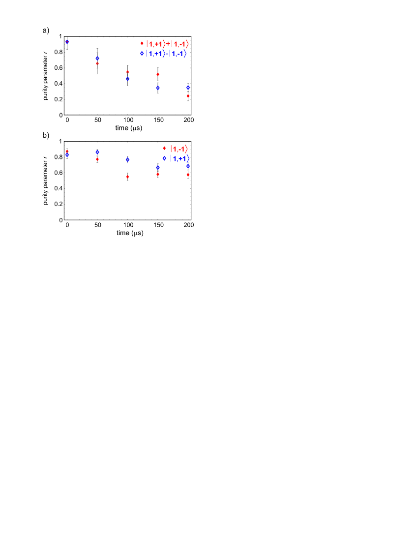
Figure 5: (Color online) Purity parameter resulting from the partial state tomography giving a lower bound for the state purity Rosenfeld08 .

In order to estimate the coherent fraction of the reconstructed spin-1 density matrices in Fig. 4 the corresponding purity parameter $r$ was evaluated according to Eq. (31), assessing a lower bound of the atomic spin-coherence. For the evolution of the superposition states $\frac{1}{\sqrt{2}}\left(\left|1,-1\right\rangle\pm\left|1,+1\right\rangle\right)$, see Fig. 5(a), we determine a $1/e$ dephasing time of $150\,\mathrm{\mu s}$. For the states $\left|1,\pm 1\right\rangle$ we estimate the longitudinal dephasing time in absence of a guiding field by extrapolation to $T_{1}\gtrsim 500\,\mathrm{\mu s}$ (see Fig. 5(b)). This value gives the time scale on which the populations of the effective spin-1/2 states $|1,-1\rangle$ and $|1,+1\rangle$ approach an equal mixture of all three spin-1 basis-states $|1,-1\rangle$, $|1,0\rangle$ and $|1,+1\rangle$.

In essence, the significantly longer longitudinal dephasing time shows that the fluctuations of the effective magnetic field are mainly along the quantization axis $z$. These fluctuations arise predominantly from the slow thermal motion of the atom in the trap where a residual circular polarization admixture leads to a position-dependent vector light-shift. The resulting dephasing leads to a decay of the off-diagonal elements of the effective spin-1/2 density matrix $\rho_{s}$ with a $1/e$ time-constant of $T_{2}^{*}=75\,\mathrm{\mu s}$. The drift into the $\left|1,0\right\rangle$ state due to magnetic fields orthogonal to the quantization axis is significantly slower.

IV Conclusion

In this paper we have studied the coherence properties of a qubit encoded in Zeeman substates of the hyperfine ground level of a single trapped ⁸⁷Rb atom. While the “fundamental” decoherence by Raman scattering of the photons from the dipole trap beam is negligible, the atomic state can dephase due to technical limitations. The main mechanisms leading to dephasing were identified as the fluctuations of stray magnetic fields and the effective magnetic field induced by the circularly polarized component of the trapping light. By analyzing the motion of the atom in the trap we have deduced the relation between the atomic temperature and the fluctuation of the effective magnetic field due to the circular admixture in the polarization of the trapping light. The dephasing of atomic memory states was then minimized by active stabilization of the external magnetic field together with an accurate setting of the polarization of the dipole trap light.

By performing a partial state tomography of the $5^{2}S_{1/2},\,F=1$ hyperfine ground level we have analyzed the dephasing of different states. The superposition states like $\frac{1}{\sqrt{2}}(\left|1,-1\right\rangle\pm\left|1,+1\right\rangle)$ show a dephasing time of $75..150\,\mathrm{\mu s}$ which is mainly limited by field fluctuations along the quantization axis. The spin states $\left|1,\pm 1\right\rangle$ are not sensitive to these fluctuations and thus show significantly longer dephasing times. Here we want to stress again that these dephasing times were measured at a magnetic field close to zero. An externally applied guiding field would induce a controlled precession of the state while suppressing the influence of fluctuations orthogonal to its axis. However, the lifting of the degeneracy of the atomic states coming along with such guiding field may reduce the fidelity of the atom-photon entanglement scheme. Additionally it also would require a synchronization of the experiment (in particular of the time period between preparation and measurement of atomic states) to the precession period.

In order to further extend the coherence time, two ways for improvement can be envisaged. On the one hand, better stability of the magnetic field can be reached by enlarging the geometry of stabilization coils, thereby reducing field gradients. These measures may be combined with passive magnetic shielding for better suppression of external magnetic fields. On the other hand, a large contribution to the dephasing of the atomic ground state $5^{2}S_{1/2},\,F=1$ results from thermal motion of the trapped atom in the state-dependent potential induced by the residual fraction of circularly polarized dipole trap light ($<1\%$). Here longer coherence times could be reached with higher accuracy of the polarization alignment of the dipole-trap light and a reduction of birefringende of the glass cell, lowering of the trap depth, and/or better cooling of the trapped atom. Improvements of such type will extend the coherence times and thus the usability of neutral atom quantum memories for future quantum repeater networks.

References

- (1) H.-J. Briegel, W. Dür, J.I. Cirac, and P. Zoller, Phys. Rev. Lett. 81, 5932 (1998).
- (2) N. Davidson, H.J. Lee, C.S. Adams, M. Kasevich, and S. Chu, Phys. Rev. Lett. 74, 1311 (1995).
- (3) S. Kuhr et al., Phys. Rev. A 72, 023406 (2005).
- (4) R. Ozeri et al., Phys. Rev. Lett. 95, 030403 (2005).
- (5) K.S. Choi, H. Deng, J. Laurat and H.J. Kimble, Nature 452, 67 (2008).
- (6) W. Rosenfeld et al., Phys. Rev. Lett. 101, 260403 (2008).
- (7) B. Zhao et al., Nature Physics 5, 95 (2009); R. Zhao, ibid, 100 (2009).
- (8) Y.O. Dudin et al., Phys. Rev. Lett. 103, 020505 (2009).
- (9) H. Specht et al., Nature 473, 190 (2011).
- (10) R. Grimm, M. Weidemüller, and Yu.B. Ovchinnikov, Adv. At. Mol. Opt. Phys. 42, 95 (2000), arXiv:physics/9902072v1 [physics.atom-ph].
- (11) K. D. Nelson et al., Nature Physics 3, 556 (2007).
- (12) I. Bloch, Nature 453, 1016 (2008).
- (13) T. Wilk et al., Phys. Rev. Lett. 104, 010502 (2010).
- (14) L. Isenhower et al., Phys. Rev. Lett. 104, 010503 (2010).
- (15) L. Förster et al., Phys. Rev. Lett. 103, 233001 (2009).
- (16) W. S. Bakr et al., Nature 462, 74 (2009).
- (17) B.B. Blinov, D.L. Moehring, L.M. Duan, C. Monroe, Nature 428, 153 (2004).
- (18) D. N. Matsukevich et al., Phys. Rev. Lett. 95, 040405 (2005).
- (19) J. Volz et al., Phys. Rev. Lett. 96, 030404 (2006).
- (20) M. Weber, J. Volz, K. Saucke, C. Kurtsiefer, and H. Weinfurter, Phys. Rev. A 73, 043406 (2006).
- (21) W. Rosenfeld, S. Berner, J. Volz, M. Weber and H. Weinfurter, Phys. Rev. Lett. 98, 050504 (2007).
- (22) W. Rosenfeld. PhD thesis, Faculty of Physics of LMU Munich (2008). http://nbn-resolving.de/urn:nbn:de:bvb:19-100300
- (23) R.A. Cline, J.D. Miller, M.R. Matthews, and D.J. Heinzen, Opt. Lett. 19, 207 (1994).
- (24) B.S. Marthur, H. Tang, and W. Harper, Phys. Rev. 171, 11 (1968); C. Cohen-Tannoudji and J. Dupont-Roc, Phys. Rev. A 5, 968 (1972).
- (25) Experiments like towardsBell09 require preservation of atomic coherence for about .
- (26) W. Rosenfeld et al., Adv. Sci. Lett 2, 469 (2009), arXiv:0906.0703v1 [quant-ph] (2009).
- (27) N. Bloembergen, E.M. Purcell, and R.V. Pound, Phys. Rev. 73, 679 (1948).
- (28) U. Leonhardt, Phys. Rev. Lett. 74, 4101 (1995); D.F.V. James, P.G. Kwiat, W.J. Munro, and A.G. White, Phys. Rev. A 64, 052312 (2001).
- (29) R.G. Newton and B.L. Young, Annals of Physics 49, 393 (1968); H.F. Hofmann and S. Takeuchi, Phys. Rev. A 69, 042108 (2004).