Variational Gaussian Process Dynamical Systems

Abstract

High dimensional time series are endemic in applications of machine learning such as robotics (sensor data), computational biology (gene expression data), vision (video sequences) and graphics (motion capture data). Practical nonlinear probabilistic approaches to this data are required. In this paper we introduce the variational Gaussian process dynamical system. Our work builds on recent variational approximations for Gaussian process latent variable models to allow for nonlinear dimensionality reduction simultaneously with learning a dynamical prior in the latent space. The approach also allows for the appropriate dimensionality of the latent space to be automatically determined. We demonstrate the model on a human motion capture data set and a series of high resolution video sequences.

1 Introduction

Nonlinear probabilistic modeling of high dimensional time series data is a key challenge for the machine learning community. A standard approach is to simultaneously apply a nonlinear dimensionality reduction to the data whilst governing the latent space with a nonlinear temporal prior. The key difficulty for such approaches is that analytic marginalization of the latent space is typically intractable. Markov chain Monte Carlo approaches can also be problematic as latent trajectories are strongly correlated making efficient sampling a challenge. One promising approach to these time series has been to extend the Gaussian process latent variable model [1, 2] with a dynamical prior for the latent space and seek a maximum a posteriori (MAP) solution for the latent points [3, 4, 5]. Ko and Fox [6] further extend these models for fully Bayesian filtering in a robotics setting. We refer to this class of dynamical models based on the GP-LVM as Gaussian process dynamical systems (GPDS). However, the use of a MAP approximation for training these models presents key problems. Firstly, since the latent variables are not marginalised, the parameters of the dynamical prior cannot be optimized without the risk of overfitting. Further, the dimensionality of the latent space cannot be determined by the model: adding further dimensions always increases the likelihood of the data. In this paper we build on recent developments in variational approximations for Gaussian processes [7, 8] to introduce a variational Gaussian process dynamical system (VGPDS) where latent variables are approximately marginalized through optimization of a rigorous lower bound on the marginal likelihood. As well as providing a principled approach to handling uncertainty in the latent space, this allows both the parameters of the latent dynamical process and the dimensionality of the latent space to be determined. The approximation enables the application of our model to time series containing millions of dimensions and thousands of time points. We illustrate this by modeling human motion capture data and high dimensional video sequences.

2 The Model

Assume a multivariate times series dataset $\{\mathbf{y}_{n},t_{n}\}_{n=1}^{N}$, where $\mathbf{y}_{n}\in\mathbb{R}^{D}$ is a data vector observed at time $t_{n}\in\mathbbm{R}_{+}$. We are especially interested in cases where each $\mathbf{y}_{n}$ is a high dimensional vector and, therefore, we assume that there exists a low dimensional manifold that governs the generation of the data. Specifically, a temporal latent function $\mathbf{x}(t)\in\mathbb{R}^{Q}$ (with $Q\ll D$), governs an intermediate hidden layer when generating the data, and the $d$th feature from the data vector $\mathbf{y}_{n}$ is then produced from $\mathbf{x}_{n}=\mathbf{x}(t_{n})$ according to

$$\mathit{y_{nd}}=f_{d}(\mathbf{x}_{n})+\epsilon_{nd}\;,\;\;\;\epsilon_{nd}\sim\mathcal{N}(0,\beta^{-1}),$$ (1)

where $f_{d}(\mathbf{x})$ is a latent mapping from the low dimensional space to $d$th dimension of the observation space and $\beta$ is the inverse variance of the white Gaussian noise. We do not want to make strong assumptions about the functional form of the latent functions $(\mathbf{x},\mathbf{f})$. Instead we would like to infer them in a fully Bayesian non-parametric fashion using Gaussian processes [9]. Therefore, we assume that $\mathbf{x}$ is a multivariate Gaussian process indexed by time $t$ and $\mathbf{f}$ is a different multivariate Gaussian process indexed by $\mathbf{x}$, and we write

$$x_{q}(t) \sim \mathcal{GP}(0,k_{x}(t_{i},t_{j})),\ \ q=1,\ldots,Q,$$ (2)

$$f_{d}(\mathbf{x}) \sim \mathcal{GP}(0,k_{f}(\mathbf{x}_{i},\mathbf{x}_{j})),\ \ d=1,\ldots,D.$$ (3)

Here, the individual components of the latent function $\mathbf{x}$ are taken to be independent sample paths drawn from a Gaussian process with covariance function $k_{x}(t_{i},t_{j})$. Similarly, the components of $\mathbf{f}$ are independent draws from a Gaussian process with covariance function $k_{f}(\mathbf{x}_{i},\mathbf{x}_{j})$. These covariance functions, parametrized by parameters $\bm{\theta}_{x}$ and $\bm{\theta}_{f}$ respectively, play very distinct roles in the model. More precisely, $k_{x}$ determines the properties of each temporal latent function $x_{q}(t)$. For instance, the use of an Ornstein-Uhlbeck covariance function yields a Gauss-Markov process for $x_{q}(t)$, while the squared-exponential kernel gives rise to very smooth and non-Markovian processes. In our experiments, we will focus on the squared exponential covariance function (RBF), the Matern $3/2$ which is only once differentiable, and a periodic covariance function [9, 10] which can be used when data exhibit strong periodicity. These kernel functions take the form:

$$k_{x(\text{rbf})}\left(\mathit{t_{i},t_{j}}\right) = \sigma_{\text{rbf}}^{2}e^{-\frac{\left(t_{i}-t_{j}\right)^{2}}{\left(2l_{t}^{2}\right)}},\ \ k_{x(\text{mat})}\left(t_{i},t_{j}\right)=\sigma_{\text{mat}}^{2}\left(1+\frac{\sqrt{3}|t_{i}-t_{j}|}{l_{t}}\right)e^{\frac{-\sqrt{3}|t_{i}-t_{j}|}{l_{t}}},$$

$$k_{x(\text{per})}\left(\mathit{t_{i},t_{j}}\right) = \sigma_{\text{per}}^{2}e^{-\frac{1}{2}\frac{sin^{2}\left(\frac{2\pi}{T}\left(t_{i}-t_{j}\right)\right)}{l_{t}}}.$$ (4)

The covariance function $k_{f}$ determines the properties of the latent mapping $\mathbf{f}$ that maps each low dimensional variable $\mathbf{x}_{n}$ to the observed vector $\mathbf{y}_{n}$. We wish this mapping to be a non-linear but smooth, and thus a suitable choice is the squared exponential covariance function

$$\mathit{k_{f}}\left(\mathbf{x}_{i},\mathbf{x}_{j}\right)={} \sigma_{ard}^{2}e^{-\frac{1}{2}\sum_{q=1}^{Q}w_{q}\left(\mathit{x_{i,q}-x_{j,q}}\right)^{2}},$$ (5)

which assumes a different scale $w_{q}$ for each latent dimension. This, as in the variational Bayesian formulation of the GP-LVM [8], enables an automatic relevance determination procedure (ARD), i.e. it allows Bayesian training to “switch off” unnecessary dimensions by driving the values of the corresponding scales to zero.

The matrix $\mathit{Y}\in\mathbb{R}^{N\times D}$ will collectively denote all observed data so that its $n$th row corresponds to the data point $\mathbf{y}_{n}$. Similarly, the matrix $F\in\mathbb{R}^{N\times D}$ will denote the mapping latent variables, i.e. $f_{nd}=f_{d}(\mathbf{x}_{n})$, associated with observations $Y$ from (1). Ana usly, $X\in\mathbb{R}^{N\times Q}$ will store all low dimensional latent variables $x_{nq}=x_{q}(t_{n})$. Further, we will refer to columns of these matrices by the vectors $\mathbf{y}_{d},\mathbf{f}_{d},\mathbf{x}_{q}\in\mathbbm{R}^{N}$. Given the latent variables we assume independence over the data features, and given time we assume independence over latent dimensions to give

$$p(Y,F,X|\mathbf{t})=p(Y|F)p(F|X)p(X|\mathbf{t})=\prod_{d=1}^{D}p(\mathbf{y}_{d}|\mathbf{f}_{d})p(\mathbf{f}_{d}|\mathit{X})\prod_{q=1}^{Q}p(\mathbf{x}_{q}|\mathbf{t}),$$ (6)

where $\mathbf{t}\in\mathbb{R}^{N}$ and $p(\mathbf{y}_{d}|\mathbf{f}_{d})$ is a Gaussian likelihood function term defined from (1). Further, $p(\mathbf{f}_{d}|\mathit{X})$ is a marginal GP prior such that

$$p(\mathbf{f}_{d}|\mathit{X})=\mathcal{N}(\mathbf{f}_{d}|\mathbf{0},\mathit{K_{NN}}),$$ (7)

where $\mathit{K}_{NN}=\mathit{k}_{f}(X,X)$ is the covariance matrix defined by the kernel function $\mathit{k}_{f}$ and similarly $p(\mathbf{x}_{q}|\mathbf{t})$ is the marginal GP prior associated with the temporal function $x_{q}(t)$,

$$p(\mathbf{x}_{q}|\mathbf{t})=\mathcal{N}\left(\mathbf{x}_{q}|\mathbf{0},\mathit{K_{t}}\right),$$ (8)

where $K_{t}=k_{x}(\mathbf{t},\mathbf{t})$ is the covariance matrix obtained by evaluating the kernel function $\mathit{k}_{x}$ on the observed times $\mathbf{t}$.

Bayesian inference using the above model poses a huge computational challenge as, for instance, marginalization of the variables $X$, that appear non-linearly inside the kernel matrix $K_{NN}$, is troublesome. Practical approaches that have been considered until now (e.g. [5, 3]) marginalise out only $F$ and seek a MAP solution for $X$. In the next section we describe how efficient variational approximations can be applied to marginalize $X$ by extending the framework of [8].

2.1 Variational Bayesian training

The key difficulty with the Bayesian approach is propagating the prior density $p(X|\mathbf{t})$ through the nonlinear mapping. This mapping gives the expressive power to the model, but simultaneously renders the associated marginal likelihood,

$$p(Y|\mathbf{t})=\int p(Y|F)p(F|X)p(X|\mathbf{t})\text{d}X\text{d}F,$$ (9)

intractable. We now invoke the variational Bayesian methodology to approximate the integral. Following a standard procedure [11], we introduce a variational distribution $q(\Theta)$ and compute the Jensen’s lower bound $\mathcal{F}_{v}$ on the logarithm of (9),

$$\mathcal{F}_{v}(q,\bm{\theta})={} \int q(\mathit{\Theta})\log\frac{p(Y|F)p(F|X)p(\mathit{X}|\mathbf{t})}{q(\mathit{\Theta})}\text{d}X\text{d}F,$$ (10)

where $\bm{\theta}$ denotes the model’s parameters. However, the above form of the lower bound is problematic becauce $X$ (in the GP term $p(F|X)$) appears non-linearly inside the kernel matrix $K_{NN}$ making the integration over $X$ difficult. As shown in [8], this intractability is removed by applying the “data augmentation” principle. More precisely, we augment the joint probability model in (6) by including $M$ extra samples of the GP latent mapping $\mathbf{f}$, known as inducing points, so that $\mathbf{u}_{m}\in\mathbb{R}^{D}$ is such a sample. The inducing points are evaluated at a set of pseudo-inputs $\tilde{X}\in\mathbb{R}^{M\times Q}$. The augmented joint probability density takes the form

$$p(Y,F,U,X,\tilde{X}|\mathbf{t})=\prod_{d=1}^{D}p(\mathbf{y}_{d}|\mathbf{f}_{d})p(\mathbf{f}_{d}|\mathbf{u}_{d},\mathit{X})p(\mathbf{u}_{d}|\tilde{X})p(X|\mathbf{t}),$$ (11)

where $p(\mathbf{u}_{d}|\tilde{X})$ is a zero-mean Gaussian with a covariance matrix $K_{MM}$ constructed using the same function as for the GP prior (7). By dropping $\tilde{X}$ from our expressions, we write the augmented GP prior analytically (see [9]) as

$$p(\mathbf{f}_{d}|\mathbf{u}_{d},X)=\mathcal{N}\left(\mathbf{f}_{d}|K_{NM}K_{MM}^{-1}\mathbf{u}_{d},K_{NN}-K_{NM}K_{MM}^{-1}K_{MN}\right).$$ (12)

A key result in [8] is that a tractable lower bound (computed analogously to (10)) can be obtained through the variational density

$$q(\mathit{\Theta})=q(F,U,X)=q(F|U,X)q(U)q(X)=\prod_{d=1}^{D}p(\mathbf{f}_{d}|\mathbf{u}_{d},X)q(\mathbf{u}_{d})q(X),$$ (13)

where $q(X)=\prod_{q=1}^{Q}\mathcal{N}\left(\mathbf{x}_{q}|\bm{\mu}_{q},S_{q}\right)$ and $q(\mathbf{u}_{d})$ is an arbitrary variational distribution. Titsias and Lawrence [8] assume full independence for $q(X)$ and the variational covariances are diagonal matrices. Here, in contrast, the posterior over the latent variables will have strong correlations, so $S_{q}$ is taken to be a $N\times N$ full covariance matrix. Optimization of the variational lower bound provides an approximation to the true posterior $p(X|Y)$ by $q(X)$. In the augmented probability model, the “difficult” term $p(F|X)$ appearing in (10) is now replaced with (12) and, eventually, it cancels out with the first factor of the variational distribution (13) so that $F$ can be marginalised out analytically. Given the above and after breaking the logarithm in (10), we obtain the final form of the lower bound (see supplementary material for more details)

$$\mathcal{F}_{v}(q,\bm{\theta})=\hat{\mathcal{F}}_{v}-\text{KL}(q(X)\parallel p(X|\mathbf{t})),$$ (14)

with $\hat{\mathcal{F}}_{v}=\int q(X)\log p(Y|F)p(F|X)\,\mathrm{d}X\text{d}F$. Both terms in (14) are now tractable. Note that the first of the above terms involves the data while the second one only involves the prior. All the information regarding data point correlations is captured in the KL term and the connection with the observations comes through the variational distribution. Therefore, the first term in (14) has the same analytical solution as the one derived in [8]. (14) can be maximized by using gradient-based methods. However, when not factorizing $q(X)$ across data points yields $O(N^{2})$ variational parameters to optimize. This issue is addressed in the next section.

2.2 Reparametrization and Optimization

The optimization involves the model parameters $\bm{\theta}=(\beta,\bm{\theta}_{f},\bm{\theta}_{t})$, the variational parameters $\{\bm{\mu}_{q},S_{q}\}_{q=1}^{Q}$ from $q(X)$ and the inducing points $\tilde{X}$.

Optimization of the variational parameters appears challenging, due to their large number and the correlations between them. However, by reparametrizing our $O\left(N^{2}\right)$ variational parameters according to the framework described in [12] we can obtain a set of $O(N)$ less correlated variational parameters. Specifically, we first take the derivatives of the variational bound (14) w.r.t. $S_{q}$ and $\bm{\mu}_{q}$ and set them to zero, to find the stationary points,

$$S_{q}=\left(\mathit{K}_{t}^{-1}+\Lambda_{q}\right)^{-1}\;\;\;\text{and}\;\;\;\bm{\mu}_{q}=K_{t}\bar{\bm{\mu}}_{q},$$ (15)

where $\Lambda_{q}=-2\frac{\vartheta\mathit{\hat{F}_{v}(q,\bm{\theta})}}{\vartheta\mathit{S_{q}}}$ is a $N\times N$ diagonal, positive matrix and $\bar{\bm{\mu}}_{q}=\frac{\vartheta\hat{F}_{v}}{\vartheta\bm{\mu}_{q}}$ is a $N-$dimensional vector. The above stationary conditions tell us that, since $S_{q}$ depends on a diagonal matrix $\Lambda_{q}$, we can reparametrize it using only the $N-$dimensional diagonal of that matrix, denoted by $\bm{\lambda}_{q}$. Then, we can optimise the $2(Q\times N)$ parameters $(\bm{\lambda}_{q}$, $\bar{\bm{\mu}}_{q})$ and obtain the original parameters using (15).

2.3 Learning from Multiple Sequences

Our objective is to model multivariate time series. A given data set may consist of a group of independent observed sequences, each with a different length (e.g. in human motion capture data several walks from a subject). Let, for example, the dataset be a group of $S$ independent sequences $\left(Y^{(1)},...,Y^{(S)}\right)$. We would like our model to capture the underlying commonality of these data. We handle this by allowing a different temporal latent function for each of the independent sequences, so that $X^{(s)}$ is the set of latent variables corresponding to the sequence $s$. These sets are a priori assumed to be independent since they correspond to separate sequences, i.e. $p\left(X^{(1)},X^{(2)},...,X^{(S)}\right)=\prod_{s=1}^{S}p(X^{(s)})$, where we dropped the conditioning on time for simplicity. This factorisation leads to a block-diagonal structure for the time covariance matrix $K_{t}$, where each block corresponds to one sequenece. In this setting, each block of observations $Y^{(s)}$ is generated from its corresponding $X^{(s)}$ according to $Y^{(s)}=F^{(s)}+\bm{\epsilon}$, where the latent function which governs this mapping is shared across all sequences and $\bm{\epsilon}$ is Gaussian noise.

3 Predictions

Our algorithm models the temporal evolution of a dynamical system. It should be capable of generating completely new sequences or reconstructing missing observations from partially observed data. For generating novel sequence given training data the model requires a time vector $\mathbf{t}_{*}$ as input and computes a density $p(Y_{*}|Y,\mathbf{t},\mathbf{t}_{*})$. For reconstruction of partially observed data the time stamp information is additionally accompanied by a partially observed sequence $Y_{*}^{p}\in\mathbb{R}^{N_{*}\times D_{p}}$ from the whole $Y_{*}=(Y_{*}^{p},Y_{*}^{m})$, where $p$ and $m$ are set of indices indicating the present (i.e. observed) and missing dimensions of $Y_{*}$ respectively, so that $p\cup m=\{1,\ldots,D\}$. We reconstruct the missing dimensions by computing the Bayesian predictive distribution $p(Y_{*}^{m}|Y_{*}^{p},Y,\mathbf{t}_{*},\mathbf{t})$. The predictive densities can also be used as estimators for tasks like generative Bayesian classification. Whilst time stamp information is always provided, in the next section we drop its dependence to avoid notational clutter.

3.1 Predictions Given Only the Test Time Points

To approximate the predictive density, we will need to introduce the underlying latent function values $F_{*}\in\mathbb{R}^{N_{*}\times D}$ (the noisy-free version of $Y_{*}$) and the latent variables $X_{*}\in\mathbb{R}^{N_{*}\times Q}$. We write the predictive density as

$$p(Y_{*}|Y) = \int p(Y_{*},F_{*},X_{*}|Y_{*},Y)\text{d}F_{*}\text{d}X_{*}=\int p(Y_{*}|F_{*})p(F_{*}|X_{*},Y)p(X_{*}|Y)\text{d}F_{*}\text{d}X_{*}.$$ (16)

The term $p(F_{*}|X_{*},Y)$ is approximated by the variational distribution

$$q(F_{*}|X_{*}) = \int\prod_{d\in D}p(\mathbf{f}_{*,d}|\mathbf{u}_{d},X_{*})q(\mathbf{u}_{d})d\mathbf{u}_{d}=\prod_{d\in D}q(\mathbf{f}_{*,d}|X_{*}),$$ (17)

where $q(\mathbf{f}_{*,d}|X_{*})$ is a Gaussian that can be computed analytically, since in our variational framework the optimal setting for $q(\mathbf{u}_{d})$ is also found to be a Gaussian (see suppl. material for complete forms). As for the term $p(X_{*}|Y)$ in eq. (16), it is approximated by a Gaussian variational distribution $q(X_{*})$,

$$q(X_{*})=\prod_{q=1}^{Q}q(\mathbf{x}_{*,q})=\prod_{q=1}^{Q}\int p(\mathbf{x}_{*,q}|\mathbf{x}_{q})q(\mathbf{x}_{q})\text{d}\mathbf{x}_{q}=\prod_{q=1}^{Q}\left\langle p(\mathbf{x}_{*,q}|\mathbf{x}_{q})\right\rangle_{q(\mathbf{x}_{q})},$$ (18)

where $p(\mathbf{x}_{*,q}|\mathbf{x}_{q})$ is a Gaussian found from the conditional GP prior (see [9]) and $q(X)$ is also Gaussian. We can, thus, work out analytically the mean and variance for (18), which turn out to be:

$$\mu_{x_{*,q}}={} K_{*N}\bar{\mu}_{q}$$ (19)

$$\text{var}(x_{*,q})={} K_{**}-K_{*N}(K_{t}+\Lambda_{q}^{-1})^{-1}K_{N*}.$$ (20)

where $K_{*N}=k_{x}(\mathbf{t}_{*},\mathbf{t})$, $K_{*N}=K_{*N}^{\top}$ and $K_{**}=k_{x}(\mathbf{t}_{*},\mathbf{t}_{*})$. Notice that these equations have exactly the same form as found in standard GP regression problems. Once we have analytic forms for the posteriors in (16), the predictive density is approximated as

$$p(Y_{*}|Y){} =\int p(Y_{*}|F_{*})q(F_{*}|X_{*})q(X_{*})\text{d}F_{*}\text{d}X_{*}=\int p(Y_{*}|F_{*})\left\langle q(F_{*}|X_{*})\right\rangle_{q(X_{*})}\text{d}F_{*},$$ (21)

which is a non-Gaussian integral that cannot be computed analytically. However, following the same argument as in [9, 13], we can calculate analytically its mean and covariance:

$$\mathbb{E}(F_{*})={} B^{\top}\Psi_{1}^{*}$$ (22)

$$\text{Cov}(F_{*})={} B^{\top}\left(\Psi_{2}^{*}-\Psi_{1}^{*}(\Psi_{1}^{*})^{\top}\right)B+\Psi_{0}^{*}I-\text{Tr}\left[\left(K_{MM}^{-1}-\left(K_{MM}+\beta\Psi_{2}\right)^{-1}\right)\Psi_{2}^{*}\right]I,$$ (23)

where $B=\beta\left(K_{MM}+\beta\Psi_{2}\right)^{-1}\Psi_{1}^{\top}Y$, $\Psi_{0}^{*}=\left\langle k_{f}(X_{*},X_{*})\right\rangle$, $\Psi_{1}^{*}=\left\langle K_{M*}\right\rangle$ and $\Psi_{2}^{*}=\left\langle K_{M*}K_{*M}\right\rangle$. All expectations are taken w.r.t. $q(X_{*})$ and can be calculated analytically, while $K_{M*}$ denotes the cross-covariance matrix between the training inducing inputs $\tilde{X}$ and $X_{*}$. The $\Psi$ quantities are calculated analytically (see suppl. material). Finally, since $Y_{*}$ is just a noisy version of $F_{*}$, the mean and covariance of (21) is just computed as: $\mathbb{E}(Y_{*})=\mathbb{E}(F_{*})$ and $\text{Cov}(Y_{*})=\text{Cov}(F_{*})+\beta^{-1}I_{N_{*}}$.

3.2 Predictions Given the Test Time Points and Partially Observed Outputs

The expression for the predictive density $p(Y_{*}^{m}|Y_{*}^{p},Y)$ is similar to (16),

$$p(Y_{*}^{m}|Y_{*}^{p},Y) = \int p(Y_{*}^{m}|F_{*}^{m})p(F_{*}^{m}|X_{*},Y_{*}^{p},Y)p(X_{*}|Y_{*}^{p},Y)\text{d}F_{*}^{m}\text{d}X_{*},$$ (24)

and is analytically intractable. To obtain an approximation, we firstly need to apply variational inference and approximate $p(X_{*}|Y_{*}^{p},Y)$ with a Gaussian distribution. This requires the optimisation of a new variational lower bound that accounts for the contribution of the partially observed data $Y_{*}^{p}$. This lower bound approximates the true marginal likelihood $p(Y_{*}^{p},Y)$ and has exactly analogous form with the lower bound computed only on the training data $Y$. Moreover, the variational optimisation requires the definition of the variational distribution $q(X_{*},X)$ which needs to be optimised and is fully correlated across $X$ and $X_{*}$. After the optimisation, the approximation to the true posterior $p(X_{*}|Y_{*}^{p},Y)$ is given from the marginal $q(X_{*})$. A much faster but less accurate method would be to decouple the test from the training latent variables by imposing the factorisation $q(X_{*},X)=q(X)q(X_{*})$. This is not used, however, in our current implementation.

4 Handling Very High Dimensional Datasets

Our variational framework avoids the typical cubic complexity of Gaussian processes allowing relatively large training sets (thousands of time points, $N$). Further, the model scales only linearly with the number of dimensions $D$. Specifically, the number of dimensions only matters when performing calculations involving the data matrix $Y$. In the final form of the lower bound (and consequently in all of the derived quantities, such as gradients) this matrix only appears in the form $YY^{\top}$ which can be precomputed. This means that, when $N\ll D$, we can calculate $YY^{\top}$ only once and then substitute $Y$ with the SVD (or Cholesky decomposition) of $YY^{\top}$. In this way, we can work with an $N\times N$ instead of an $N\times D$ matrix. Practically speaking, this allows us to work with data sets involving millions of features. In our experiments we model directly the pixels of HD quality video, exploiting this trick.

5 Experiments

We consider two different types of high dimensional time series, a human motion capture data set consisting of different walks and high resolution video sequences. The experiments are intended to explore the various properties of the model and to evaluate its performance in different tasks (prediction, reconstruction, generation of data). Matlab source code for repeating the following experiments is available on-line from http://staffwww.dcs.shef.ac.uk/people/N.Lawrence/vargplvm/.

5.1 Human Motion Capture Data

We followed [14, 15] in considering motion capture data of walks and runs taken from subject 35 in the CMU motion capture database. We treated each motion as an independent sequence. The data set was constructed and preprocessed as described in [15]. This results in 2,613 separate 59-dimensional frames split into 31 training sequences with an average length of 84 frames each.

The model is jointly trained, as explained in section 2.3, on both walks and runs, i.e. the algorithm learns a common latent space for these motions. At test time we investigate the ability of the model to reconstruct test data from a previously unseen sequence given partial information for the test targets. This is tested once by providing only the dimensions which correspond to the body of the subject and once by providing those that correspond to the legs. We compare with results in [15], which used MAP approximations for the dynamical models, and against nearest neighbour. We can also indirectly compare with the binary latent variable model (BLV) of [14] which used a slightly different data preprocessing. We assess the performance using the cumulative error per joint in the scaled space defined in [14] and by the root mean square error in the angle space suggested by [15]. Our model was initialized with nine latent dimensions. We performed two runs, once using the Matern covariance function for the dynamical prior and once using the RBF. From table 1 we see that the variational Gaussian process dynamical system considerably outperforms the other approaches. The appropriate latent space dimensionality for the data was automatically inferred by our models. The model which employed an RBF covariance to govern the dynamics retained four dimensions, whereas the model that used the Matern kept only three. The other latent dimensions were completely switched off by the ARD parameters. The best performance for the legs and the body reconstruction was achieved by the VGPDS model that used the Matern and the RBF covariance function respectively.

Table 1: Errors obtained for the motion capture dataset considering nearest neighbour in the angle space (NN) and in the scaled space(NN sc.), GPLVM, BLV and VGPDS. CL / CB are the leg and body datasets as preprocessed in [14], L and B the corresponding datasets from [15]. SC corresponds to the error in the scaled space, as in Taylor et al. while RA is the error in the angle space. The best error per column is in bold.

Data	CL	CB	L	L	B	B
Error Type	SC	SC	SC	RA	SC	RA
BLV	11.7	8.8	-	-	-	-
NN sc.	22.2	20.5	-	-	-	-
GPLVM (Q = 3)	-	-	11.4	3.40	16.9	2.49
GPLVM (Q = 4)	-	-	9.7	3.38	20.7	2.72
GPLVM (Q = 5)	-	-	13.4	4.25	23.4	2.78
NN sc.	-	-	13.5	4.44	20.8	2.62
NN	-	-	14.0	4.11	30.9	3.20
VGPDS (RBF)	-	-	8.19	3.57	10.73	1.90
VGPDS (Matern 3/2)	-	-	6.99	2.88	14.22	2.23

5.2 Modeling Raw High Dimensional Video Sequences

For our second set of experiments we considered video sequences. Such sequences are typically preprocessed before modeling to extract informative features and reduce the dimensionality of the problem. Here we work directly with the raw pixel values to demonstrate the ability of the VGPDS to model data with a vast number of features. This also allows us to directly sample video from the learned model.

Firstly, we used the model to reconstruct partially observed frames from test video sequences. For the first video discussed here we gave as partial information approximately 50% of the pixels while for the other two we gave approximately 40% of the pixels on each frame. The mean squared error per pixel was measured to compare with the $k-$nearest neighbour (NN) method, for $k\in(1,..,5)$ (we only present the error achieved for the best choice of $k$ in each case). The datasets considered are the following: firstly, the ‘Missa’ dataset, a standard benchmark used in image processing. This is 103,680-dimensional video, showing a woman talking for 150 frames. The data is challenging as there are translations in the pixel space. We also considered an HD video of dimensionality $9\times 10^{5}$ that shows an artificially created scene of ocean waves as well as a $230,400-$dimensional video showing a dog running for $60$ frames. The later is approximately periodic in nature, containing several paces from the dog. For the first two videos we used the Matern and RBF kernel respectively to model the dynamics and interpolated to reconstruct blocks of frames chosen from the whole sequence. For the ‘dog’ dataset we constructed a compound kernel $k_{x}=k_{x(\text{rbf})}+k_{x(\text{periodic})}$, where the RBF term is employed to capture any divergence from the approximately periodic pattern. We then used our model to reconstruct the last 7 frames extrapolating beyond the original video. As can be seen in table 2, our method outperformed NN in all cases. The results are also demonstrated visually in figure 1 and the reconstructed videos are available in the supplementary material.

Table 2: The mean squared error per pixel for VGPDS and NN for the three datasets (measured only in the missing inputs). The number of latent dimensions selected by our model is in parenthesis.

	Missa	Ocean	Dog
VGPDS	2.52 ($Q=12$)	9.36 ($Q=9$)	4.01 ($Q=6$)
NN	2.63	9.53	4.15

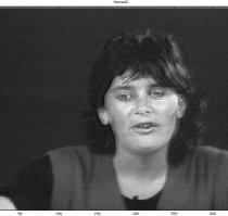
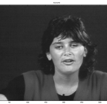
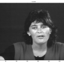
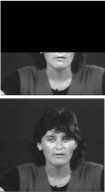
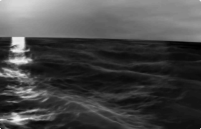
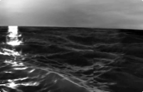
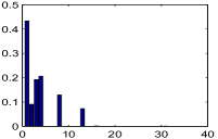
Figure 1: 1 and 1 demonstrate the reconstruction achieved by VGPDS and NN respectively for the most challenging frame 1 of the ‘missa’ video, i.e. when translation occurs. 1 shows another example of the reconstruction achieved by VGPDS given the partially observed image. 1 (VGPDS) and 1 (NN) depict the reconstruction achieved for a frame of the ‘ocean’ dataset. Finally, we demonstrate the ability of the model to automatically select the latent dimensionality by showing the initial lengthscales (fig: 1) of the ARD kernel and the values obtained after training (fig: 1) on the ‘dog’ data set.

As can be seen in figure 1, VGPDS predicts pixels which are smoothly connected with the observed image, whereas the NN method cannot fit the predicted pixels in the overall context.

As a second task, we used our generative model to create new samples and generate a new video sequence. This is most effective for the ‘dog’ video as the training examples were approximately periodic in nature. The model was trained on 60 frames (time-stamps $[t_{1},t_{60}]$) and we generated the new frames which correspond to the next 40 time points in the future. The only input given for this generation of future frames was the time stamp vector, $[t_{61},t_{100}]$. The results show a smooth transition from training to test and amongst the test video frames. The resulting video of the dog continuing to run is sharp and high quality. This experiment demonstrates the ability of the model to reconstruct massively high dimensional images without blurring. Frames from the result are shown in figure 2. The full video is available in the supplementary material.

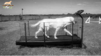
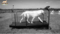
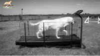
Figure 2: The last frame of the training video 2 is smoothly followed by the first frame 2 of the generated video. A subsequent generated frame can be seen in 2.

6 Discussion and Future Work

We have introduced a fully Bayesian approach for modeling dynamical systems through probabilistic nonlinear dimensionality reduction. Marginalizing the latent space and reconstructing data using Gaussian processes results in a very generic model for capturing complex, non-linear correlations even in very high dimensional data, without having to perform any data preprocessing or exhaustive search for defining the model’s structure and parameters.

Our method’s effectiveness has been demonstrated in two tasks; firstly, in modeling human motion capture data and, secondly, in reconstructing and generating raw, very high dimensional video sequences. A promising future direction to follow would be to enhance our formulation with domain-specific knowledge encoded, for example, in more sophisticated covariance functions or in the way that data are being preprocessed. Thus, we can obtain application-oriented methods to be used for tasks in areas such as robotics, computer vision and finance.

Acknowledgments

Research was partially supported by the University of Sheffield Moody endowment fund and the Greek State Scholarships Foundation (IKY). We also thank Colin Litster and “Fit Fur Life” for allowing us to use their video files as datasets.

Appendix

Appendix A Derivation of the variational bound

We wish to approximate the marginal likelihood:

$$p(Y|\mathbf{t})=\int p(Y,F,X|\mathbf{t})\text{d}X\text{d}F,$$ (25)

by computing a lower bound:

$$\mathcal{F}_{v}(q,\bm{\theta})={} \int q(\mathit{\Theta})\log\frac{p(Y,F,\mathit{X}|\mathbf{t})}{q(\mathit{\Theta})}\text{d}X\text{d}F,$$ (26)

This can be achieved by first augmenting the joint probability density of our model with inducing inputs $\tilde{X}$ along with their corresponding function values $U$:

$$p(Y,F,U,X,\tilde{X}|\mathbf{t})=\prod_{d=1}^{D}p(\mathbf{y}_{d}|\mathbf{f}_{d})p(\mathbf{f}_{d}|\mathbf{u}_{d},\mathit{X})p(\mathbf{u}_{d}|\tilde{X})p(X|\mathbf{t})$$ (27)

where $p(\mathbf{u}_{d}|\tilde{X})=\prod_{d=1}^{D}\mathcal{N}\left(\mathbf{u}_{d}|\mathbf{0},K_{MM}\right)$ . For simplicity, $\tilde{X}$ is dropped from our expressions for the rest of this supplementary material. Note that after including the inducing points, $p(\mathbf{f}_{d}|\mathbf{u}_{d},X)$ remains analytically tractable and it turns out to be [9]):

$$p(\mathbf{f}_{d}|\mathbf{u}_{d},X)=\mathcal{N}\left(\mathbf{f}_{d}|K_{NM}K_{MM}^{-1}\mathbf{u}_{d},K_{NN}-K_{NM}K_{MM}^{-1}K_{MN}\right).$$ (28)

We are now able to define a variational distribution $q(\Theta)$ which factorises as: For tractability we now define a variational density, $q(\Theta)$:

$$q(\mathit{\Theta})=q(F,U,X)=q(F|U,X)q(U)q(X)=\prod_{d=1}^{D}p(\mathbf{f}_{d}|\mathbf{u}_{d},X)q(\mathbf{u}_{d})q(X),$$ (29)

where $q(X)=\prod_{q=1}^{Q}\mathcal{N}\left(\mathbf{x}_{q}|\bm{\mu}_{q},S_{q}\right)$. Now, we return to (26) and replace the joint distribution with its augmented version (27) and the variational distribution with its factorised version (29):

$$\mathcal{F}_{v}(q,\bm{\theta})={} \int q(\mathit{\Theta})\log\frac{p(Y,F,U,X|\mathbf{t})}{q(F,U,X)}\text{d}X\text{d}F,$$

$$={} \int\prod_{d=1}^{D}p(\mathbf{f}_{d}|\mathbf{u}_{d},X)q(\mathbf{u}_{d})q(X)\log\frac{\prod_{d=1}^{D}p(\mathbf{y}_{d}|\mathbf{f}_{d})\cancel{p(\mathbf{f}_{d}|\mathbf{u}_{d},\mathit{X})}p(\mathbf{u}_{d}|\tilde{X})p(X|\mathbf{t})}{\prod_{d=1}^{D}\cancel{p(\mathbf{f}_{d}|\mathbf{u}_{d},X)}q(\mathbf{u}_{d})q(X))}\text{d}X\text{d}F$$

$$={} \int\prod_{d=1}^{D}p(\mathbf{f}_{d}|\mathbf{u}_{d},X)q(\mathbf{u}_{d})q(X)\log\frac{\prod_{d=1}^{D}p(\mathbf{y}_{d}|\mathbf{f}_{d})p(\mathbf{u}_{d}|\tilde{X})}{\prod_{d=1}^{D}q(\mathbf{u}_{d})q(X))}\text{d}X\text{d}F,$$

$$-{} \int\prod_{d=1}^{D}q(X)\log\frac{q(X)}{p(X|\mathbf{t})}\text{d}X$$

$$={} \hat{\mathcal{F}}_{v}-\text{KL}(q\parallel p),$$ (30)

with $\hat{\mathcal{F}}_{v}=\int q(X)\log p(Y|F)p(F|X)\,\mathrm{d}X\text{d}F=\sum_{d=1}^{D}\hat{\mathcal{F}}_{d}$. Both terms in (30) are analytically tractable, with the first having the same analytical solution as the one derived in [8]. Further calculations in the the $\hat{\mathcal{F}}_{v}$ term reveal that the optimal setting for $q(\mathbf{u}_{d})$ is also a Gaussian. More specifically, we have:

$$\hat{\mathcal{F}}_{v}={} \int q(\mathbf{u}_{d})\log\frac{e^{\left\langle\log N\left(\mathbf{y}_{d}|\mathbf{a}_{d},\beta^{-1}I_{d}\right)\right\rangle_{q(X)}}p(\mathbf{u}_{d})}{q(\mathbf{u}_{d})}d\mathbf{u}_{d}-A$$ (31)

where $A$ is a collection of remaining terms and $\mathbf{a}_{d}$ is the mean of (28). (31) is a KL-like quantity and, therefore, $q(\mathbf{u}_{d})$ is optimally set to be the quantity appearing in the numerator of the above equation. So:

$$q(\mathbf{u}_{d})=e^{\left\langle\log\mathcal{N}\left(\mathbf{y}_{d}|\mathbf{a}_{d},\beta^{-1}I_{d}\right)\right\rangle_{q(X)}}p(\mathbf{u}_{d}),$$

exactly as in [8]. This is a Gaussian distribution since $p(\mathbf{u}_{d})=\mathcal{N}(\mathbf{u}_{d}|\mathbf{0},K_{MM})$.

The complete form of the jensen’s lower bound turns out to be:

$$\mathcal{F}_{v}(q,\bm{\theta})={} \sum_{d=1}^{D}\hat{\mathcal{F}}_{d}(q,\bm{\theta})-\text{KL}(q\parallel p)$$

$$={} \sum_{d=1}^{D}\log\left(\frac{(\beta)^{\frac{N}{2}}|\mathit{K_{MM}}|^{\frac{1}{2}}}{(2\pi)^{\frac{N}{2}}|\beta\Psi_{2}+\mathit{K_{MM}}|^{\frac{1}{2}}}e^{-\frac{1}{2}\mathbf{y}^{T}_{d}W\mathbf{y}_{d}}\right)-\frac{\beta\psi_{0}}{2}+\frac{\beta}{2}\text{Tr}\left(\mathit{K_{MM}^{-1}}\Psi_{2}\right)$$

$$-\frac{Q}{2}\log|\mathit{K_{t}}|-\frac{1}{2}\sum_{q=1}^{Q}\left[\text{Tr}\left(\mathit{K_{t}}^{-1}\mathit{S_{q}}\right)+\text{Tr}\left(\mathit{K_{t}}^{-1}\bm{\mu}_{q}\bm{\mu}_{q}^{T}\right)\right]+\frac{1}{2}\sum_{q=1}^{Q}\log|\mathit{S_{q}}|+const$$ (32)

where the last line corresponds to the KL term. Also:

$$\Psi_{0}=\text{Tr}(\langle\mathit{K_{NN}}\rangle_{q(\mathit{X})})\;,\;\;\Psi_{1}=\langle\mathit{K_{NM}}\rangle_{q(\mathit{X})}\;,\;\;\Psi_{2}=\langle\mathit{K_{MN}}\mathit{K_{NM}}\rangle_{q(\mathit{X})}$$ (33)

The $\Psi$ quantities can be computed analytically as in [8].

Appendix B Derivatives of the variational bound

Before giving the expressions for the derivatives of the variational bound (30), it should be reminded that the variational parameters $\mu_{q}$ and $S_{q}$ (for all $q$s) have been reparametrised as $S_{q}=\left(\mathit{K}_{t}^{-1}+diag(\bm{\lambda}_{q})\right)^{-1}\text{ and }\bm{\mu}_{q}=K_{t}\bar{\bm{\mu}}_{q}$, where the function $diag(\cdot)$ transforms a vector into a square diagonal matrix and vice versa. Given the above, the set of the parameters to be optimised is $(\bm{\theta}_{f},\bm{\theta}_{x},\{\bar{\bm{\mu}}_{q},\bm{\lambda}_{q}\}_{q=1}^{Q},\tilde{X}$. The gradient w.r.t the inducing points $\tilde{X}$, however, has exactly the same form as for $\bm{\theta}_{f}$ and, therefore, is not presented here. Also notice that from now on we will often use the term “variational parameters” to refer to the new quantities $\bar{\bm{\mu}}_{q}$ and $\bm{\lambda}_{q}$.

Some more notation:

1. $\lambda_{q}$ is a scalar, an element of the vector $\bm{\lambda}_{q}$ which, in turn, is the main diagonal of the diagonal matrix $\Lambda_{q}$.

2. $S_{ij}\triangleq S_{q;ij}$ the element of $S_{q}$ found in the $i$-th row and $j$-th column.

3. $\mathbf{s}_{q}\triangleq\{S_{q;ii}\}_{i=1}^{N}$, i.e. it is a vector with the diagonal of $S_{q}$.

B.1 Derivatives w.r.t the variational parameters

$$\frac{\vartheta\mathcal{F}_{v}}{\vartheta\bar{\bm{\mu}}_{q}}=K_{t}\left(\frac{\vartheta\hat{\mathcal{F}}}{\vartheta\bm{\mu}_{q}}-\bar{\bm{\mu}}_{q}\right)\text{ and }\frac{\vartheta\mathcal{F}_{v}}{\vartheta\bm{\lambda}_{q}}=-(S_{q}\circ S_{q})\left(\frac{\vartheta\hat{\mathcal{F}}}{\vartheta\mathbf{s}_{q}}+\frac{1}{2}\bm{\lambda}_{q}\right).$$ (34)

where:

$$\frac{\hat{\mathcal{F}}(q,\bm{\theta})}{\vartheta\mu_{q}}{} =-\frac{\beta D}{2}\frac{\vartheta\Psi_{0}}{\vartheta\mu_{q}}+\beta\text{Tr}\left(\frac{\vartheta\Psi_{1}^{T}}{\vartheta\mu_{q}}YY^{T}\Psi_{1}A^{-1}\right)$$

$$+\frac{\beta}{2}\text{Tr}\left[\frac{\vartheta\Psi_{2}}{\vartheta\mu_{q}}\left(DK_{MM}^{-1}-\beta^{-1}DA^{-1}-A^{-1}\Psi_{1}^{T}YY^{T}\Psi_{1}A^{-1}\right)\right]$$ (35)

$$\frac{\vartheta\hat{\mathcal{F}}(q,\bm{\theta})}{\vartheta S_{q;i,j}}{} =-\frac{\beta D}{2}\frac{\vartheta\Psi_{0}}{\vartheta S_{q;i,j}}+\beta\text{Tr}\left(\frac{\vartheta\Psi_{1}^{T}}{\vartheta S_{q;i,j}}YY^{T}\Psi_{1}A^{-1}\right)$$

$$+\frac{\beta}{2}\text{Tr}\left[\frac{\vartheta\Psi_{2}}{\vartheta S_{q;i,j}}\left(DK_{MM}^{-1}-\beta^{-1}DA^{-1}-A^{-1}\Psi_{1}^{T}YY^{T}\Psi_{1}A^{-1}\right)\right]$$ (36)

with $A=\beta^{-1}K_{MM}+\Psi_{2}$.

B.2 Derivatives w.r.t $\bm{\theta}=(\bm{\theta}_{f},\bm{\theta}_{x})$ and $\beta$

Given that the KL term involves only the temporal prior, its gradient w.r.t the parameters $\bm{\theta}_{f}$ is zero. Therefore:

$$\frac{\vartheta\mathcal{F}_{v}}{\vartheta\theta_{f}}=\frac{\vartheta\hat{\mathcal{F}}}{\vartheta\theta_{f}}$$ (37)

with:

$$\frac{\vartheta\hat{\mathcal{F}}}{\vartheta\theta_{f}}{} =\text{const}-\frac{\beta D}{2}\frac{\vartheta\Psi_{0}}{\vartheta\theta_{f}}+\beta\text{Tr}\left(\frac{\vartheta\Psi_{1}^{T}}{\vartheta\theta_{f}}YY^{T}\Psi_{1}A^{-1}\right)$$

$$+\frac{1}{2}\text{Tr}\left[\frac{\vartheta K_{MM}}{\vartheta\theta_{f}}\left(DK_{MM}^{-1}-\beta^{-1}DA^{-1}-A^{-1}\Psi_{1}^{T}YY^{T}\Psi_{1}A^{-1}-\beta DK_{MM}^{-1}\Psi_{2}K_{MM}^{-1}\right)\right]$$

$$+\frac{\beta}{2}\text{Tr}\left[\frac{\vartheta\Psi_{2}}{\vartheta\theta_{f}}\;\;\;\;\left(DK_{MM}^{-1}-\beta^{-1}DA^{-1}-A^{-1}\Psi_{1}^{T}YY^{T}\Psi_{1}A^{-1}\right)\right]$$ (38)

The expression above is identical for the derivatives w.r.t the inducing points. For the gradients w.r.t the $\beta$ term, we have a similar expression:

$$\frac{\vartheta\hat{\mathcal{F}}}{\vartheta\beta}={} \frac{1}{2}\Big{[}D\left(\text{Tr}(K_{MM}^{-1}\Psi_{2})+(N-M)\beta^{-1}-\Psi_{0}\right)-\text{Tr}(YY^{\top})+\text{Tr}(A^{-1}\Psi_{1}^{\top}YY^{\top}\Psi_{1})$$

$$+{} \beta^{-2}D\text{Tr}(K_{MM}A^{-1})+\beta^{-1}\text{Tr}\left(K_{MM}^{-1}A^{-1}\Psi_{1}^{\top}YY^{\top}\Psi_{1}A^{-1}\right)\Big{]}$$ (39)

In contrast to the above, the term $\hat{\mathcal{F}}_{v}$ does involve parameters $\bm{\theta}_{x}$, because it involves the variational parameters that are now reparametrized with $K_{t}$, which in turn depends on $\bm{\theta}_{x}$. To demonstrate that, we will forget for a moment the reparametrization of $S_{q}$ and we will express the bound as $F(\bm{\theta}_{x},\mu_{q}(\bm{\theta}_{x}))$ (where $\mu_{q}(\bm{\theta}_{x})=K_{t}\bar{\bm{\mu}_{q}}$) so as to show explicitly the dependency on the variational mean which is now a function of $\bm{\theta}_{x}$. Our calculations must now take into account the term $\left(\frac{\vartheta\hat{\mathcal{F}}(\bm{\mu}_{q})}{\vartheta\bm{\mu}_{q}}\right)^{\top}\frac{\vartheta\mu_{q}(\bm{\theta}_{x})}{\vartheta\bm{\theta}_{x}}$ that is what we “miss” when we consider $\mu_{q}(\bm{\theta}_{x})=\bm{\mu}_{q}$:

$$\frac{\vartheta\mathcal{F}_{v}(\bm{\theta}_{x},\mu_{q}(\bm{\theta}_{x}))}{\vartheta\theta_{x}}={} \frac{\vartheta\mathcal{F}_{v}(\bm{\theta}_{x},\bm{\mu}_{q})}{\vartheta\theta_{x}}+\left(\frac{\vartheta\hat{\mathcal{F}}(\bm{\mu}_{q})}{\vartheta\bm{\mu}_{q}}\right)^{\top}\frac{\vartheta\mu_{q}(\bm{\theta}_{x})}{\vartheta\theta_{x}}$$

$$={} \cancel{\frac{\vartheta\hat{\mathcal{F}}(\bm{\mu}_{q})}{\vartheta\theta_{x}}}+\frac{\vartheta(-\text{KL})(\bm{\theta}_{x},\bm{\mu}_{q}(\bm{\theta}_{x}))}{\vartheta\theta_{x}}+\left(\frac{\vartheta\hat{\mathcal{F}}(\bm{\mu}_{q})}{\vartheta\bm{\mu}_{q}}\right)^{\top}\frac{\vartheta\mu_{q}(\bm{\theta}_{x})}{\vartheta\theta_{x}}$$ (40)

We do the same for $S_{q}$ and then we can take the resulting equations and replace $\bm{\mu}_{q}$ and $S_{q}$ with their equals so as to take the final expression which only contains $\bar{\bm{\mu}}_{q}$ and $\bm{\lambda}_{q}$:

$$\frac{\vartheta\mathcal{F}_{v}(\bm{\theta}_{x},\mu_{q}(\bm{\theta}_{x}),S_{q}(\bm{\theta}_{x}))}{\vartheta\theta_{x}}={} \text{Tr}\bigg{[}\Big{[}-\frac{1}{2}\left(\hat{B}_{q}K_{t}\hat{B}_{q}+\bar{\bm{\mu}}_{q}\bar{\bm{\mu}}_{q}^{\top}\right)$$

$$+{} \left(I-\hat{B}_{q}K_{t}\right)diag\left(\frac{\vartheta\hat{\mathcal{F}}}{\vartheta\mathbf{s}_{q}}\right)\left(I-\hat{B}_{q}K_{t}\right)^{\top}\Big{]}\frac{\vartheta K_{t}}{\vartheta\theta_{x}}\bigg{]}$$

$$+{} \left(\frac{\vartheta\hat{\mathcal{F}}(\bm{\mu}_{q})}{\vartheta\bm{\mu}_{q}}\right)^{\top}\frac{\vartheta K_{t}}{\vartheta\theta_{x}}\bar{\bm{\mu}}_{q}$$ (41)

where $\hat{B}_{q}=\Lambda_{q}^{\frac{1}{2}}\widetilde{B}_{q}^{-1}\Lambda_{q}^{\frac{1}{2}}$. and $\tilde{B}_{q}=I+\Lambda_{q}^{\frac{1}{2}}K_{t}\Lambda_{q}^{\frac{1}{2}}$. Note that by using this $\tilde{B}_{q}$ matrix (which has eigenvalues bounded below by one) we have an expression which, when implemented, leads to more numerically stable computations, as explained in [9] page 45-46.

Appendix C Predictions

C.1 Predictions given only the test time points

To approximate the predictive density, we will need to introduce the underlying latent function values $F_{*}\in\mathbb{R}^{N_{*}\times D}$ (the noisy-free version of $Y_{*}$) and the latent variables $X_{*}\in\mathbb{R}^{N_{*}\times Q}$. We write the predictive density as

$$p(Y_{*}|Y) = \int p(Y_{*},F_{*},X_{*}|Y_{*},Y)\text{d}F_{*}\text{d}X_{*}=\int p(Y_{*}|F_{*})p(F_{*}|X_{*},Y)p(X_{*}|Y)\text{d}F_{*}\text{d}X_{*}.$$ (42)

The term $p(F_{*}|X_{*},Y)$ is approximated according to

$$q(F_{*}|X_{*}) = \int\prod_{d\in D}p(\mathbf{f}_{*,d}|\mathbf{u}_{d},X_{*})q(\mathbf{u}_{d})\text{d}\mathbf{u}_{d}=\prod_{d\in D}q(\mathbf{f}_{*,d}|X_{*}),$$ (43)

where $q(\mathbf{f}_{*,d}|X_{*})$ is a Gaussian that can be computed analytically.The term $p(X_{*}|Y)$ in eq. (42) is approximated by a Gaussian variational distribution $q(X_{*})$,

$$p(X_{*}|Y)\approx{} \int p(X_{*}|X)q(X)\text{d}X=\left\langle p(X_{*}|X)\right\rangle_{q(X)}=q(X_{*})=\prod_{q=1}^{Q}q(\mathbf{x}_{*,q}),$$ (44)

where $p(X_{*,q}|X)$ can be found from the conditional GP prior (see [9]). We can then write

$$\mathbf{x}_{*,q}=\bm{\alpha}\mathbf{x}_{q}+\bm{\epsilon},$$ (45)

where $\bm{\alpha}=K_{*N}K_{t}^{-1}$ and $\bm{\epsilon}\sim\mathcal{N}\left(\mathbf{0},K_{**}-K_{*NK_{t}^{-1}K_{N*}}\right)$. Also, $K_{t}=k_{x}(\mathbf{t},\mathbf{t})$, $K_{*N}=k_{x}(\mathbf{t}_{*},\mathbf{t})$ and $K_{**}=k_{x}(\mathbf{t}_{*}\mathbf{t}_{*})$. Given the above, we know a priori that (44) is a Gaussian and by taking expectations over $q(X)$ in the r.h.s. of (45) we find the mean and covariance of $q(X_{*})$. Substituting for the equivalent forms of $\bm{\mu}_{q}$ and $S_{q}$ from section 2.2 we obtain the final solution

$$\mu_{x_{*,q}}={} \mathbf{k}_{*N}\bar{\mu}_{q}$$ (46)

$$\text{var}(x_{*,q})={} k_{**}-\mathbf{k}_{*N}(K_{t}+\Lambda_{q}^{-1})^{-1}\mathbf{k}_{N*}.$$ (47)

(42) can then be written as:

$$p(Y_{*}|Y){} =\int p(Y_{*}|F_{*})q(F_{*}|X_{*})q(X_{*})\text{d}F_{*}\text{d}X_{*}=\int p(Y_{*}|F_{*})\left\langle q(F_{*}|X_{*})\right\rangle_{q(X_{*})}\text{d}F_{*}$$ (48)

Although the expectation appearing in the above integral is not a Gaussian, its moments can be found analytically [9, 13],

$$\mathbb{E}(F_{*})={} B^{\top}\Psi_{1}^{*}$$ (49)

$$\text{Cov}(F_{*})={} B^{\top}\left(\Psi_{2}^{*}-\Psi_{1}^{*}(\Psi_{1}^{*}){\top}\right)B+\Psi_{0}^{*}I-\text{Tr}\left[\left(K_{MM}^{-1}-\left(K_{MM}+\beta\Psi_{2}\right)^{-1}\right)\Psi_{2}^{*}\right]I,$$ (50)

where $B=\beta\left(K_{MM}+\beta\Psi_{2}\right)^{-1}\Psi_{1}^{\top}Y$, $\Psi_{0}^{*}=\left\langle k_{f}(X_{*},X_{*})\right\rangle$, $\Psi_{1}^{*}=\left\langle K_{M*}\right\rangle$ and $\Psi_{2}^{*}=\left\langle K_{M*}K_{*M}\right\rangle$. All expectations are taken w.r.t. $q(X_{*})$ and can be calculated analytically, while $K_{M*}$ denotes the cross-covariance matrix between the training inducing inputs $\tilde{X}$ and $X_{*}$. Finally, since $Y_{*}$ is just a noisy version of $F_{*}$, the mean and covariance of (48) is just computed as: $\mathbb{E}(Y_{*})=\mathbb{E}(F_{*})$ and $\text{Cov}(Y_{*})=\text{Cov}(F_{*})+\beta^{-1}I_{N_{*}}$.

C.2 Predictions given the test time points and partially observed outputs

The expression for the predictive density $p(Y_{*}^{m}|Y_{*}^{p},Y)$ follows exactly as in section C.1 but we need to compute probabilities for $Y_{*}^{m}$ instead of $Y_{*}$ and $Y$ is replaced with $(Y,Y_{*}^{p})$ in all conditioning sets. Similarly, $F$ is replaced with $F^{m}$. Now $q(X_{*})$ cannot be found analytically as in section C.1; instead, it is optimised so that $Y_{*}^{p}$ are taken into account. This is done by maximising the variational lower bound on the marginal likelihood:

$$p(Y_{*}^{p},Y)={} \int p(Y_{*}^{p},Y|X_{*},X)p(X_{*},X)\text{d}X_{*}\text{d}X$$

$$={} \int p(Y^{m}|X)p(Y_{*}^{p},Y^{p}|X_{*},X)p(X_{*},X)\text{d}X_{*}\text{d}X,$$

Notice that here, unlike the main paper, we work with the likelihood after marginalising $F$, for simplicity. Assuming a variational distribution $q(X_{*},X)$ and using Jensen’s inequality we obtain the lower bound

$$\int q(X_{*},X)\log\frac{p(Y^{m}|X)p(Y_{*}^{p},Y^{p}|X_{*},X)p(X_{*},X)}{q(X_{*},X)}\text{d}X_{*}\text{d}X$$ (51)

$$= \int q(X)\log p(Y^{m}|X)\text{d}X+\int q(X_{*},X)\log p(Y_{*}^{p},Y^{p}|X_{*},X)\text{d}X_{*}\text{d}X$$

$$- \text{KL}[q(X_{*},X)||p(X_{*},X)]$$

This quantity can now be maximized in the same manner as for the bound of the training phase. Unfortunately, this means that the variational parameters that are already optimised from the training procedure cannot be used here because $X$ and $X_{*}$ are coupled in $q(X_{*},X)$. A much faster but less accurate method would be to decouple the test from the training latent variables by imposing the factorisation $q(X_{*},X)=q(X)q(X_{*})$. Then, equation (51) would break into terms containing $X$, $X_{*}$ or both. The ones containing only $X$ could then be treated as constants.

Appendix D Additional results from the experiments

Figure 3: The values of the scales of the ARD kernel after training on the motion capture dataset using the RBF (fig: 3) and the Matern (fig: 3) kernel to model the dynamics for VGPDS. The scales that have zero value “switch off” the corresponding dimension of the latent space. The latent space is, therefore, 3-D for 3 and 4-D for 3. Note that the scales were initialized with very similar values.

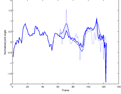
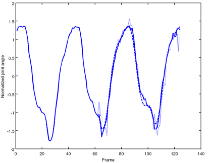
Figure 4: The prediction for two of the test angles for the body (fig: 4) and for the legs part (fig: 4). Continuous line is the original test data, dotted line is nearest neighour in scaled space, dashed line is VGPDS (using the RBF kernel for the body reconstruction and the Matern for the legs).

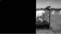
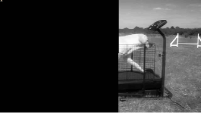
Figure 5: Some more examples for the reconstruction achieved for the ‘dog’ dataset. $40\%$ of the test image’s pixels (figures 5 and 5) were presented to the model, which was able to successfully reconstruct them, as can be seen in 5 and 5.

References

• [1] N. D. Lawrence, “Probabilistic non-linear principal component analysis with Gaussian process latent variable models,” Journal of Machine Learning Research, vol. 6, pp. 1783–1816, 2005.
• [2] N. D. Lawrence, “Gaussian process latent variable models for visualisation of high dimensional data,” in In NIPS, p. 2004, 2004.
• [3] J. M. Wang, D. J. Fleet, and A. Hertzmann, “Gaussian process dynamical models,” in In NIPS, pp. 1441–1448, MIT Press, 2006.
• [4] J. M. Wang, D. J. Fleet, and A. Hertzmann, “Gaussian process dynamical models for human motion,” IEEE Transactions on Pattern Analysis and Machine Intelligence, vol. 30, pp. 283–298, Feb. 2008.
• [5] N. D. Lawrence, “Hierarchical Gaussian process latent variable models,” in In International Conference in Machine Learning, 2007.
• [6] J. Ko and D. Fox, “GP-BayesFilters: Bayesian filtering using Gaussian process prediction and observation models,” Auton. Robots, vol. 27, pp. 75–90, July 2009.
• [7] M. Titsias, “Variational learning of inducing variables in sparse Gaussian processes,” JMLR W&CP, vol. 5, pp. 567–574, 2009.
• [8] M. Titsias and N. D. Lawrence, “Bayesian Gaussian process latent variable model,” Journal of Machine Learning Research - Proceedings Track, vol. 9, pp. 844–851, 2010.
• [9] C. E. Rasmussen and C. Williams, Gaussian Processes for Machine Learning. MIT Press, 2006.
• [10] D. J. C. MacKay, “Introduction to Gaussian processes,” in Neural Networks and Machine Learning (C. M. Bishop, ed.), NATO ASI Series, pp. 133–166, Kluwer Academic Press, 1998.
• [11] C. M. Bishop, Pattern Recognition and Machine Learning (Information Science and Statistics). Springer, 1st ed. 2006. corr. 2nd printing ed., Oct. 2007.
• [12] M. Opper and C. Archambeau, “The variational Gaussian approximation revisited,” Neural Computation, vol. 21, no. 3, pp. 786–792, 2009.
• [13] A. Girard, C. E. Rasmussen, J. Quiñonero-Candela, and R. Murray-Smith, “Gaussian process priors with uncertain inputs - application to multiple-step ahead time series forecasting,” in Neural Information Processing Systems, 2003.
• [14] G. W. Taylor, G. E. Hinton, and S. Roweis, “Modeling human motion using binary latent variables,” in Advances in Neural Information Processing Systems, p. 2007, MIT Press, 2006.
• [15] N. D. Lawrence, “Learning for larger datasets with the Gaussian process latent variable model,” Journal of Machine Learning Research - Proceedings Track, vol. 2, pp. 243–250, 2007.