Josephson-like currents in graphene for arbitrary time-dependent potential barriers

Abstract

From the exact solution of the Dirac-Weyl equation we find unusual currents $j_{y}$ running in $y$-direction parallel to a time-dependent scalar potential barrier $W(x,t)$ placed upon a monolayer of graphene, even for vanishing momentum component $p_{y}$. In their sine-like dependence on the phase difference of wave functions, describing left and right moving Dirac fermions, these currents resemble Josephson currents in superconductors, including the occurance of Shapiro steps at certain frequencies of potential oscillations. The Josephson-like currents are calculated for several specific time-dependent barriers. A novel type of resonance is discovered when, accounting for the Fermi velocity, temporal and spatial frequencies match.

1 Introduction

Growing interest to graphene, see e.g. Ref. Novoselov05 ; review , is stimulated by many unusual and sometimes counterintuitive properties of this two dimensional material. Indeed, graphene supplies charge carriers exhibiting the pseudo-relativistic dynamics of massless Dirac fermions. One example of the unusual dynamics of electrons and holes in graphene is the Klein tunneling phenomenon paradox which occurs with unit probability through arbitrarily high and thick barriers at perpendicular incidence, irrespective of the particle energy, in accordance with experiment paradox-exp . In consequence, the question arose of how to control the electron motion in graphene and hence boosted detailed studies of Dirac fermions under the influence of various forms of scalar superl ; super5 ; left ; peeters09b ; laser1 ; laser2 ; Efetov ; pnexperiments or vector magstruc potentials.

So far, many of works were devoted to studies of graphene subject to static periodic electric fields, since these structures known as graphene superlattices superl ; super5 allow controlling both spectrum and transport properties of electrons in graphene. For instance, it was shown super5 that 1D graphene superlattices have a deep analogy with photonic crystals formed by alternating right-handed and left-handed transparent media, similar as the earlier stated analogy left of a p-n junction in graphene to a Veselago lens. Superlattices of electrostatic periodic potentials can be used to collimate the directional spread of electron beams in graphene peeters09b so that waves of small transverse momentum will dominate transport properties.

Applying a time-dependent laser field to a pristine graphene sample opens an alternative and efficient way laser1 ; laser2 ; Efetov to control spectrum and transport properties of graphene samples. It has been shown that changing the time dependence of laser fields can mimic laser2 the influence of any electrostatic graphene superlattices on the electron spectrum in graphene. Further, Dirac fermions in graphene superlattices can aquire an effective mass proportional to the frequency of an applied laser field, accompanied with an exponential suppression of chiral tunneling even for perpendicular incidence upon the barrier laser2 ; Efetov , which is in stark contrast to Klein tunneling occuring in the absence of the laser field. Studies of how electron transport in graphene is affected by time-and-space dependent potentials are yet limited. Recently, it was shown our_prl that even scalar potential barriers can produce resonant amplification of reflections when modulated at proper frequencies. Moreover, an unusual current running parallel to the barrier $W(x,t)$ in $y$-direction has been predicted our_prl for electrons at zero $y$-component of the electron momentum.

In this article we study in detail this unusual Josephson-like current for electrons traveling at zero transverse momentum, $p_{y}=0$, accross a time-dependent potential barrier $W(x,t)$, assumed as homogeneous along the $y$-direction. Explicit calculations reveal Shapiro steps for properly chosen frequencies and/or electron momentum in a full analogy to the Josephson current arising through an irradiated barrier between two superconductors. We also show that this Josephson-like current in graphene can assume a non-zero dc-component, resemble the ac-Josephson effect, and/or be strongly enhanced at certain spatio-temporal matching conditions. Experimental test of our predictions should be within reach of present day nanostructure design on graphene pnexperiments . Note, that a somewhat related effect, an unusual ballistic side-jump motion of electrons and holes, has been predicted schliemann to occur in semiconductor quantum wells as a result of Rashba spin-orbit coupling.

2 Exact solution for a scalar potential of arbitrary space and time dependence

The honeycomb lattice of graphene engenders two copies, $\tau_{z}=\pm 1$, of Dirac-Weyl Hamiltonians kanemele

$$H_{0}=v_{\mbox{\tiny F}}\>[\hat{\tau}_{z}\hat{\sigma}_{x}\hat{p}_{x}+\hat{\sigma}_{y}\hat{p}_{y}]\;,$$ (1)

centered about two inequivalent Dirac points (“valleys”) $K$ and $K^{\prime}$ at corners of the hexagonal first Brillouin zone where electron-hole symmetric bands touch; here Pauli matrices $\hat{\sigma}_{x,y,z}$ act on two-component spinors representing sublattice amplitudes, exhibiting opposite Fermion helicities, $\>\bm{\sigma}\cdot\bm{p}/p=\pm 1\>$. SU(2) rotations with respect to the vector $\bm{\hat{\tau}}$ of three Pauli matrices allow to continuously transform both copies into one another beenakker08 which motivated the terminus “valleytronics” for isospin manipulations based on eigenstates to $\hat{\tau}_{z}$, Ref. rycerz07 , in analogy to the well-known research area of spintronics wolf01 . Proposals exist to valley polarize carriers, by means of nanoribbons terminated by zig-zag edges rycerz07 ; akhmerov08 ; peeters09 , by exploiting trigonal warping at elevated energies garcia08 , or by absorbing magnetic textures ziegler10 .

Below, we focus on valley polarized situations. Indeed, smooth electromagnetic or disorder potentials do not couple the two valleys ando98 , so that calculations can be done independently, for either $\tau_{z}=+1$ or $\tau_{z}=-1$. Including now the barrier potential $W(x,t)$ the Dirac equation becomes

$$v_{\mbox{\tiny F}}(\tau_{z}\hat{p}_{x}-{\rm i}\hat{p}_{y})\Psi_{B}+\hbar W(x,t)\Psi_{A}={\rm i}\hbar\frac{\partial\Psi_{A}}{\partial t}$$ (2)

$$v_{\mbox{\tiny F}}(\tau_{z}\hat{p}_{x}+{\rm i}\hat{p}_{y})\Psi_{A}+\hbar W(x,t)\Psi_{B}={\rm i}\hbar\frac{\partial\Psi_{B}}{\partial t}\;,$$

where the wave functions $\Psi_{A},\Psi_{B}$ describe electrons on either of the hexagonal graphene sublattices, $v_{\mbox{\tiny F}}$ is the Fermi velocity, and the momentum operator is defined as $(\hat{p}_{x},\hat{p}_{y})=(-{\rm i}\hbar\partial/\partial x,-{\rm i}\hbar\partial/\partial y)$. This equation has been solved analytically for time-independent potentials, for rectangular barriers paradox , for trapezoidal barriers sonin09 , or for smooth barriers by the WKB method cheianov06 ; silvestrov07 ; fistul08 . Additional time dependent harmonic oscillations have been considered, either of gate voltages applied to each side of the rectangular barrier bjoern07 , or of an electric field imposed parallel to the barrier Efetov , or treated in resonance approximation laser2 . Recently, the exact solution for $p_{y}=0$ our_prl ; solomon has been derived which allows our_prl to uncover new physical phenomena from spatio-temporal dynamics.

To keep this article self contained we briefly repeat the crucial steps to obtain the exact solution of eq. (2) for $p_{y}=0$ and arbitrary potential $W(x,t)$ acting at positive times, i.e. $\>W(x,t<0)=0\>$. The wave functions $\Psi_{A}$ and $\Psi_{B}$ depend on time $t$ and on the coordinate $x$ across the barrier, but not on the $y$-coordinate. This simplifies (2) to read

$$-{\rm i}v_{\mbox{\tiny F}}\tau_{z}\frac{\partial\Psi_{B}}{\partial x}+W(x,t)\Psi_{A}={\rm i}\frac{\partial\Psi_{A}}{\partial t}$$ (3)

$$-{\rm i}v_{\mbox{\tiny F}}\tau_{z}\frac{\partial\Psi_{A}}{\partial x}+W(x,t)\Psi_{B}={\rm i}\frac{\partial\Psi_{B}}{\partial t}\;.$$

To solve (3) we use the Ansatz

$$\psi_{\pm}(x,t)=\frac{1}{2}\left({{\rm e}^{{\rm i}S_{\pm}(x,t)}\atop\pm\tau_{z}{\rm e}^{{\rm i}S_{\pm}(x,t)}}\right)$$ (4)

where the $\pm$ signs distinguish right and left propagating solutions. Inserting (4) into (3) results in

$$\partial_{t}S_{\pm}(x,t)\pm v_{\mbox{\tiny F}}\partial_{x}S_{\pm}(x,t)+W(x,t)=0\;.$$ (5)

This first order partial differential equation can be solved by the method of characteristics couranthilbert , yielding

$$S_{\pm}(x,t)=S_{\pm}^{(0)}(x\mp v_{\mbox{\tiny F}}t,0)-\int_{0}^{t}{\rm d}t^{\prime}\;W(x\mp v_{\mbox{\tiny F}}(t-t^{\prime}),t^{\prime})$$ (6)

explicitly in terms of $W(x,t)$. In view of (4) the term $S_{\pm}^{(0)}(x,0)$ describes the initial wave function $\psi_{\pm}(x,0)$ at time $t=0$ which, in the absence of the barrier at $t<0$, can be, for example, a plane wave of wave number $k$ in the $x$-direction, $\>S_{\pm}^{(0)}(x,0)=\pm kx\>$, or some wave packets. Then eq. (6), together with (4), describes the full solution for $t>0$

$$\psi(x,t)=a_{+}(x-v_{\mbox{\tiny F}}t)\left(1\atop\tau_{z}\right){\rm e}^{-{\rm i}\int_{0}^{t}{\rm d}t^{\prime}\;W(x-v_{\mbox{\tiny F}}(t-t^{\prime}),t^{\prime})}$$

$$\;\mbox{}+a_{-}(x+v_{\mbox{\tiny F}}t)\left(1\atop-\tau_{z}\right){\rm e}^{-{\rm i}\int_{0}^{t}{\rm d}t^{\prime}\;W(x+v_{\mbox{\tiny F}}(t-t^{\prime}),t^{\prime})}$$ (7)

where $\>a_{\pm}(x)={\rm e}^{{\rm i}S_{\pm}^{(0)}(x)}/2=[\Psi_{A}(x,t=0)\pm\tau_{z}\Psi_{B}(x,t=0)]/2\>$ encodes the initial condition. In particular, if the wave packet is initially purely right moving, $\>a_{-}=0\>$, according to (2), it continues propagating to the right at times $t>0$ with undistorted density distribution $\>|a_{+}(x-v_{\mbox{\tiny F}}t)|^{2}\>$ without reflection, acquiring at most a phase factor. However, the situation becomes more intriguing when we consider a superposition of left and right moving waves.

3 Current density perpendicular and parallel to the barrier

Next we evaluate the current density

$$j_{x}(x,t)=v_{\mbox{\tiny F}}\psi^{*}(x,t)\tau_{z}\hat{\sigma}_{x}\psi(x,t)$$

$$j_{y}(x,t)=v_{\mbox{\tiny F}}\psi^{*}(x,t)\hat{\sigma}_{y}\psi(x,t)$$ (8)

for $p_{y}=0$. Before coming to remarkably nontrivial consequences from (2) below, let us first study the $x$-component of the current density, flowing perpendicular to the barrier,

$$j_{x}(x,t)=2v_{\mbox{\tiny F}}\left(|a_{+}(x-v_{\mbox{\tiny F}}t)|^{2}-|a_{-}(x+v_{\mbox{\tiny F}}t)|^{2}\right)\;,$$ (9)

which is solely determined by the initial conditions and is independent of $W(x,t)$. An initially purely right moving wave packet, $a_{-}=0$, generates an undistorted current density peak $j_{x}=v_{\mbox{\tiny F}}|a_{+}(x-v_{\mbox{\tiny F}}t)|^{2}/2$ moving at $v_{\mbox{\tiny F}}$ towards the right. According to (9), right and left movers in the initial wave will just add their contributions to the current density of opposite sign. This confirms the finding of perfect Klein tunneling through a barrier $W(x,t)$ of any space and even any time dependence. Furthermore, the current $j_{x}$ does not depend on $\tau_{z}$, giving the same contribution from states near both valleys $K$ and $K^{\prime}$. Regarding the current normal to the barrier we find so far no unusual effects arising from the superposition of right and left moving amplitudes.

Surprisingly, although we consider electron momenta $p_{y}=0$, we find a nonzero value for the current component $j_{y}$ parallel to the barrier,

$$j_{y}(x,t) = 4\tau_{z}v_{\mbox{\tiny F}}|a_{+}(x-v_{\mbox{\tiny F}}t)a_{-}(x+v_{\mbox{\tiny F}}t)|$$ (10)

$$\times \sin\left[S_{+}(x,t)-S_{-}(x,t)\right]\;.$$

While eq. (10) vanishes for unidirectional wave packets, $j_{y}$ becomes nonzero for superpositions of left and right moving amplitudes, $\>a_{+}\neq 0\>$ and $\>a_{-}\neq 0\>$. Note that any initial density peak arising from some voltage pulse will generically contain simultaneously left and right moving amplitudes. It is this superposition which causes the qualitatively new phenomenon of a current along the barrier, exhibiting striking properties as described in the following. The sine-dependence in (10) is reminiscent of the Josephson effect where it originates from the spatial overlap of superconducting order parameters in the leads of a Josephson junction. Similarly, $j_{y}$ in graphene originates here due to overlapping amplitudes of left and right moving fermions.

Contrary to its $x$-component, the $y$-component of the current manifests a nontrivial space and time dependence. The latter also depends on $\tau_{z}$. Therefore, the best way to observe $j_{y}$ is to prepare a valley-polarized system. For non- or partly polarized situations one should add the current contribution from the second valley, yielding a total current $j_{y}(x,t)={\cal P}j_{y}^{K}(x,t)+(1-{\cal P})j_{y}^{K^{\prime}}(x,t)$ where $j_{y}^{K}$ and $j_{y}^{K^{\prime}}$ refer to states near $K$ and $K^{\prime}$ points, respectively, and ${\cal P}$ measures the degree of valley polarization such that ${\cal P}=1$ or $0$ corresponds to complete polarization and ${\cal P}=1/2$ to the unpolarized situation. Since the contribution from the other Dirac point $K^{\prime}$ can compensate the current from $K$, measuring $j_{y}$ allows to determine the degree ${\cal P}$ of valley polarization of a graphene sample.

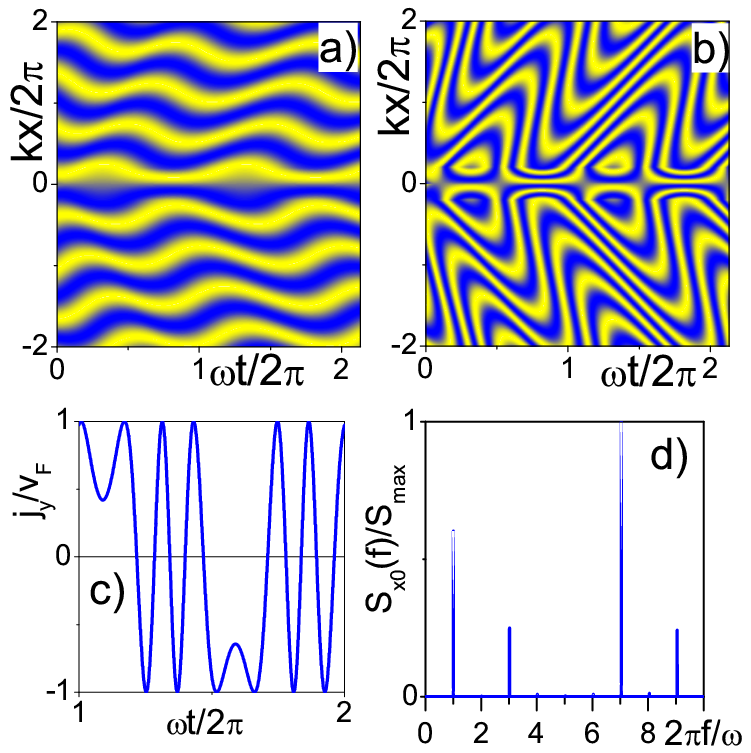
Figure 1: (Color online) Contour plot of $j_{y}(x,t)$ for the case of an oscillating square-well potential (12). Bright (yellow): $j_{y}>0$, dark (blue): $j_{y}<0$, as calculated using eq. (13) for small $W_{0}/\omega=1.75$, panel a), and for large $W_{0}/\omega=10.7$, b). The other parameters ($v_{\mbox{\tiny F}}/(L\omega)=2.35,\ kL=1.27$) are the same for all panels a)–d). With growing $W_{0}$, a wave-like structure seen in a) changes towards a more complicated pattern b) of $j_{y}$. Panel c) display cross sections $j_{y}(x_{0},t)$ of b) at $x_{0}/L=1$. Current periodicity seen in c) is consistent with the spectrum ${\cal S}_{x_{0}}(f)$, as defined in (14) (normalized by its maximum value) containing only integer harmonics as shown in panel d).

On the other hand, the current variance in $y$-direction,

$$\langle\hat{j}_{y}^{2}\rangle-\langle\hat{j}_{y}\rangle^{2} = v_{\mbox{\tiny F}}^{2}\Bigl{[}1-16|a_{+}|^{2}|a_{-}|^{2}$$

$$\times \sin^{2}\left(S_{+}(x,t)-S_{-}(x,t)\right)\Bigr{]}$$

$$= v_{\mbox{\tiny F}}^{2}[1-j_{y}^{2}(x,t)/v_{\mbox{\tiny F}}^{2}]$$

does not depend on $\tau_{z}$. In (3) we have defined the current operator $\>\hat{j}_{y}:=v_{\mbox{\tiny F}}\hat{\sigma}_{y}\>$. Even without valley polarization they remain nonzero and can be measured.

4 Josephson-like current flowing along the barrier

For valley-polarized situations, $\tau_{z}=1$ and ${\cal P}=1$, we now investigate specific examples $W(x,t)$ and substantiate the analogy between the current $j_{y}$ and a superconducting Josephson current. We consider potentials of amplitudes $W_{0}$, varying spatially on lengths scales $L$, and oscillate at frequency $\omega$ such that they vanish on time average. As initial condition we assume a superposition of right and left propagating plane waves of equal amplitudes, $\>S_{\pm}^{(0)}=\pm kx\>$.

4.1 Square well of width $2L$

Let us first consider a single square well barrier

$$W(x,t)=W_{0}\>\Theta(L-|x|)\>\sin\omega t$$ (12)

of thickness $2L$ and amplitude $W_{0}$, oscillating at frequency $\omega$. Substituting this potential in eq. (6) and using eq. (10), we derive

$$\textstyle j_{y}(x,t)=v_{\mbox{\tiny F}}\>\left\{\begin{array}[]{ll}\textstyle\sin 2\left[kx-\frac{W_{0}}{\omega}{\rm sgn}(x)\>\sin^{2}\left(\frac{\omega t}{2}-\frac{\omega}{2v_{\mbox{\tiny F}}}\bigl{|}L-|x|\bigr{|}\right)\right]&,\quad t<(L+|x|)/v_{\mbox{\tiny F}}\\ \textstyle\sin 2\left[kx-\frac{W_{0}}{\omega}{\rm sgn}(x)\>\sin\left(\frac{\omega}{v_{\mbox{\tiny F}}}\left\{{|x|\atop L}\right\}\right)\>\sin\left(\omega t-\frac{\omega}{v_{\mbox{\tiny F}}}\left\{{L\atop|x|}\right\}\right)\right]&,\quad t\geq(L+|x|)/v_{\mbox{\tiny F}}\end{array}\right.\;,$$ (13)

where the curley brackets in the sine arguments of the lower line refer to $\left\{{|x|<L\atop|x|>L}\right\}$. Fig. 1 shows $j_{y}(x,t)$ for small (1a) and large (1b) amplitude of the potential barrier. With growing $W_{0}$ an initial wave-like structure transforms into a more complicated spatio-temporal pattern. However, as seen in 1c for fixed $x_{0}$, the current $j_{y}(x_{0},t)$ remains periodic in time, as confirmed by the spectrum

$${\cal S}_{x_{0}}(f)=\left|\int_{0}^{\infty}{\rm d}t\;j_{y}(x_{0},t)\exp(2\pi{\rm i}ft)\right|^{2}$$ (14)

of $j_{y}$ at fixed $x_{0}$, showing peaks in Fig. 1d only at integer harmonics.

4.2 Homogeneous electric field

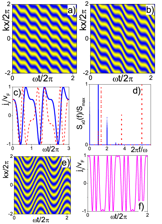
Figure 2: (Color online) Contour plot of $j_{y}(x,t)$ for an oscillating homogeneous electric field (15) at the Shapiro step $n=2$ corresponding to $W_{0}/\omega=0.86,\ v_{\mbox{\tiny F}}/L\omega=1.16$, panel a), and away from Shapiro steps ($W_{0}/\omega=0.76,\ v_{\mbox{\tiny F}}/L\omega=1.03$), b). Bright (yellow): $j_{y}>0$, dark (blue): $j_{y}<0$, calculated by using eq. (16) for $kL=1.27$. A very regular pattern is seen in a) while the pattern is more “frustrated” in b). Panel c) displays cross sections of $j_{y}(x_{0},t)$ at fixed $kx_{0}=1.27$ for the first Shapiro step (solid blue line, $W_{0}/\omega=0.61,\ v_{\mbox{\tiny F}}/L\omega=0.82$) and away from Shapiro steps (dashed red line, $W_{0}/\omega=0.75,\ v_{\mbox{\tiny F}}/L\omega=1$). At the Shapiro step, clear periodic behavior is seen, in contrast to aperiodic oscillations away from Shapiro steps. This is consistent with the spectra (normalized w.r.t. the peak maximum), cf. eq. (14), shown in panel d) where only integer harmonics contribute to the solid blue line while dashed red contains incommensurate harmonics. Contour plot of $j_{y}(x,t)$ for the oscillating homogeneous electric field (19) e), calculated by using eq. (20) for $kL=1.27,\ W_{0}/\omega=1.75,\ v_{\mbox{\tiny F}}/L\omega=2.35$. Panel f) displays the cross section of e) at $x_{0}=0.5$ which clearly exhibits now always time periodicity of $j_{y}(x_{0},t)$ for this case.

We next consider an ac-electric field with amplitude $W_{0}/L$ and frequency $\omega$ described by the potential

$$W(x,t)=\frac{W_{0}x}{L}\sin\omega t\;.$$ (15)

For this case, we derive

$$\textstyle j_{y}(x,t)=v_{\mbox{\tiny F}}\>\sin 2\left[kx+\frac{W_{0}v_{\mbox{\tiny F}}}{L}\left(\frac{t}{\omega}-\frac{\sin\omega t}{\omega^{2}}\right)\right]$$ (16)

from eqs. (6) and (10). Now $j_{y}$ may either follow the periodicity $\omega$ of (15) or it may behave aperiodically, compare the 2D contour plots in Fig. 2a and 2b. To see the non-periodicity of Fig. 2b more clearly, we plot in Fig. 2c cross sections $j_{y}(x_{0},t)$ at fixed $x_{0}$ for both cases: the solid blue line, referring to Fig. 2a, is clearly periodic, while the dashed red line, referring to 2b, is aperiodic. Corresponding spectra (Fig. 2d) reveal the same information: in the solid blue case they contain only integer harmonics while the non-integer contributions (dashed red) describe aperiodicity. We can rewrite eq. (16) as a sum

$$j_{y}(x,t) = v_{\mbox{\tiny F}}\sum_{n=-\infty}^{\infty}J_{n}\left(\frac{2W_{0}v_{\mbox{\tiny F}}}{\omega^{2}L}\right)$$ (17)

$$\times \sin\left(2kx+\frac{2W_{0}v_{\mbox{\tiny F}}t}{\omega L}-n\omega t\right)$$

using Bessel functions $J_{n}$. The last equation reveals that at $\omega=\omega_{n}$ with

$$\omega_{n}=\sqrt{2W_{0}v_{\mbox{\tiny F}}/(Ln)}\;,\quad n\in\mathbb{N}$$ (18)

and integer $n$, the $y$-component of the current exhibits a peculiarity, similar to the so-called Shapiro steps tinkham of an irradiated Josephson junction. As seen in Fig. 2c and 2d, frequencies $\omega=\omega_{n}$ generate periodic oscillations, which, again as in the case of Shapiro-steps, can induce a nonzero dc-component of the current at given $x_{0}$. Here, we remind of the statement of the previous section, that non-zero dc-currents allow to measure the degree of valley polarization. In view of eqs. (16,17) the overall dc-current vanishes after averaging over $x_{0}$ due to the harmonic $x$-dependence of $j_{y}$. Modulating the homogeneous electric field at $\omega\neq\omega_{n}$ results in aperiodic oscillations (Fig. 2b,c,d) and zero dc-component.

When we consider the same potential, seemingly just phase shifted in time,

$$W(x,t)=\frac{W_{0}x}{L}\cos\omega t\>,$$ (19)

instead of eq. (16) this yields

$$\textstyle j_{y}(x,t)=v_{\mbox{\tiny F}}\>\sin 2\left[kx+\frac{2W_{0}v_{\mbox{\tiny F}}}{\omega^{2}L}\>\sin^{2}\frac{\omega t}{2}\right]$$ (20)

without a term proportional to $t$ in the square bracket argument of the sine-functions and therefore without similarity to Shapiro steps in Josephson junctions. The oscillations of $j_{y}$ now are always periodic (as seen in Fig. 2e), though $j_{y}$ could be quite complicated (see for example Fig. 2f). For this case there is no dc-component of $j_{y}$ at any $x$. The reason for this qualitatively different behaviour as compared to (16) lies in the discontinuity of (19) at time zero (we recall that we assume $\>W(x,t<0)=0\>$), contrary to (15), so that (19) does not simply correspond to a temporal phase shift. In the limit $\>\omega\to 0\>$ the effect of a homogeneous electric field becomes time-independent for both forms (15) and (19).

4.3 Spatially and temporally periodic potentials

Now we focus on potentials which are both, periodic in space (with period $2\pi L$) and in time (with period $2\pi/\omega$). First consider

$$W(x,t)=W_{0}\cos(x/L)\>\cos(\omega t)\;.$$ (21)

Intriguingly, this potential facilitates spatio-temporal mode matching. In this case, the phase $\phi=S_{+}-S_{-}$ describing the Josephson-like current $j_{y}\propto\sin(\phi)$ varies as

$$\phi=S_{+}-S_{-} = 2kx-\frac{4W_{0}Lv_{\mbox{\tiny F}}\sin(\frac{x}{L})}{\omega^{2}L^{2}-v_{\mbox{\tiny F}}^{2}}$$

$$\times \sin\left[\frac{\omega L+v_{\mbox{\tiny F}}}{2L}t\right]\>\sin\left[\frac{\omega L-v_{\mbox{\tiny F}}}{2L}t\right]\;.$$

In this case, oscillations of $j_{y}$ persist even when $\omega\rightarrow 0$ since the static potential of spatial periodicity $L$ induces a frequency component $v_{\mbox{\tiny F}}/L$ to electron waves moving at uniform velocity $v_{\mbox{\tiny F}}$ which produces phase oscillations

$$\phi=2kx-\frac{4W_{0}L}{v_{\mbox{\tiny F}}}\sin\left(\frac{x}{L}\right)\sin^{2}\left(\frac{v_{\mbox{\tiny F}}}{2L}t\right)\;.$$ (23)

This reminds of the ac-Josephson effect tinkham where ac-current oscillations are generated by a time-independent voltage. By contrast, the potential

$$W(x,t)=W_{0}\cos(x/L)\>\sin(\omega t)$$ (24)

is continuous in time, yielding a phase

$$\phi=2kx-\frac{2W_{0}L\sin(\frac{x}{L})}{\omega^{2}L^{2}-v_{\mbox{\tiny F}}^{2}}\left(\omega L\sin\left(\frac{v_{\mbox{\tiny F}}t}{L}\right)-v_{\mbox{\tiny F}}\sin(\omega t)\right)$$ (25)

that vanishes when $\>\omega\to 0\>$ with no ac-Josephson-like effect. The essential difference (including presence or absence of the ac-Josephson-like effect) in the time dependence of $j_{y}$ for (21) and (24) is again related to the continuity of the potentials at $t=0$.

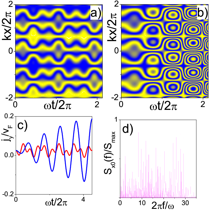
Figure 3: (Color online) Contour plot of $j_{y}(x,t)$ for an oscillating periodic potential (21), away from spatio-temporal matching resonance a), cf. eq. (4.3) ($v_{\mbox{\tiny F}}/L\omega=2.35,\ W_{0}/\omega=1.75$) and at resonance b), cf. eq. (27) ($v_{\mbox{\tiny F}}/L\omega=1,\ W_{0}/\omega=1.75$). Bright (yellow): $j_{y}>0$, dark (blue): $j_{y}<0$. Near resonance, amplitude and frequency of $j_{y}(x_{0},t)$-oscillations increase with time, as seen in c) for fixed $kx_{0}=0.0127$ for the nearly resonant case in blue ($v_{\mbox{\tiny F}}/L\omega=1.1,\ W_{0}/\omega=1.75$), compared to the case away from resonance in red ($v_{\mbox{\tiny F}}/L\omega=2.35,\ W_{0}/\omega=1.75$), where oscillations stay small. Panel d) shows the spectrum for large amplitude $W_{0}/\omega=10.7$ of the potential (21) at $kx_{0}=1.27$ for the non-resonant situation $v_{\mbox{\tiny F}}/L\omega=2.35$: now many harmonics contribute, also at frequencies much higher than $\omega/2\pi$. Such types of spectra are known rakh to enable signal amplification.

On the other hand, when $\>\omega\rightarrow v_{\mbox{\tiny F}}/L$, spatio-temporal matching occurs so that both of the previous solutions vary proportional to $t$, resulting in Josephson-like currents

$$j_{y}=v_{\mbox{\tiny F}}\sin\Bigl{(}2kx-t\,W_{0}\sin(x/L)\sin(\omega t)\Bigr{)}$$ (26)

for potential (21) and

$$j_{y}=v_{\mbox{\tiny F}}\sin\Bigl{(}2kx+t\,W_{0}\sin(x/L)\cos(\omega t)\Bigr{)}$$ (27)

for the potential in (24). As a result, $j_{y}$ amplifies with time. Indeed, for small values $W_{0}|\sin(x_{0}/L)|$ the amplitude of $j_{y}(x_{0},t)$ oscillations grows resonantly within times $t\lesssim 2\pi/(W_{0}|\sin(x_{0}/L)|)$, before it saturates, while the “effective” frequency of the oscillations keeps increasing with time. We mention here the analogy to resonant excitations of plasmonic oscillations (Wood’s anomaly woods ) by spatio-temporal matching of the incident light with the grating period. Fig. 3 depicts contour plots of $j_{y}(x,t)$ to illustrate this spatio-temporal mode matching for potential (21): panel 3a away from resonance and 3b at resonance, $\omega=v_{\mbox{\tiny F}}/L$. In the latter case the initially slowly varying structure is seen to “accelerate” as time increases. Resonant amplification of $j_{y}(x_{0},t)$ is shown in Fig. 3c for fixed $x_{0}$ and small $W_{0}|\sin(x/L)|$ (blue line); away from resonance (red line) $j_{y}(x_{0},t)$ stays small.

While at small $W_{0}$ only few harmonics contribute to the spectrum of $j_{y}(x_{0},t)$ their number and also the corresponding frequency range considerably increases at large $W_{0}$, particularly in the non-resonant case $\omega\neq v_{\mbox{\tiny F}}/L$. This is demonstrated in Fig. 3d. Those types of spectra, containing dense frequency components over a wide range of frequencies, can be employed for parametric amplification of a weak signal (encoded in small variations of the amplitude $W_{0}$) by a strong drive (large amplitude $W_{0}$) rakh .

Finally, we discuss a spatial Shapiro-step peculiarity arising in (4.3) due to the interplay of a linearly increasing term $\sim kx$ and an oscillatory term $\sim\sin(x/L)$ in $\phi$. At fixed time $t_{0}$ the current density $j_{y}(x,t_{0})\propto\sin\phi$ becomes spatially periodic whenever the Shapiro-step condition

$$k=k_{n}=\frac{n}{L}\quad,\quad n\in\mathbb{N}$$ (28)

is met for the $x$-component of the electron momentum $k$. Otherwise, $j_{y}(x,t_{0})$ behaves aperiodic in space. Interestingly, the resonance condition (28) can imply a nonzero spatial average $\langle j_{y}\rangle(t_{0})$ for the current density of electrons with momentum $k=k_{n}$.

4.4 Traveling wave potential

Let us finally consider a potential

$$W(x,t)=W_{0}\sin\frac{x-v_{0}t}{L}\;,$$ (29)

describing a traveling wave which can be generated by running monochromatic electromagnetic waves. Using equation (6) we derive

$$\phi=2\Biggl{[}kx-\frac{W_{0}L}{(v_{0}^{2}-v_{\mbox{\tiny F}}^{2})}\Bigl{[}v_{\mbox{\tiny F}}\Bigl{(}\cos\frac{x-v_{0}t}{L}$$ (30)

$$\mbox{}-\cos\frac{x-v_{\mbox{\tiny F}}t}{L}\Bigr{)}-(v_{0}-v_{\mbox{\tiny F}})\sin\frac{x}{L}\>\sin\frac{v_{\mbox{\tiny F}}t}{L}\Bigr{]}\Biggr{]}\;,$$

from which we expect a competition between the velocities $v_{0}$ and $v_{\mbox{\tiny F}}$. In the resonant case, $\>v_{0}\rightarrow v_{\mbox{\tiny F}}\>$, the phase $\phi=\>S_{+}-S_{-}\>$ grows proportional to time $t$,

$$\phi=2kx-t\;W_{0}\sin\frac{x-v_{\mbox{\tiny F}}t}{L}+\frac{W_{0}L}{v_{\mbox{\tiny F}}}\sin\frac{x}{L}\sin\frac{v_{\mbox{\tiny F}}t}{L}$$ (31)

and we find again a behavior resembling the Wood’s anomaly. However, from comparing equations (26) and (27) with equation (31) is seen that the non-propagating wave (21) comes with node-like points in space, where $\sin(x/L)=0$ and the dynamics of Josephson-like current is frozen. By contrast, the running wave potential (29) shows non-trivial dynamics of $j_{y}$ everywhere (there are no nodes of $j_{y}$ in this case). As a result, the contour plots Fig. 4a,b resemble the corresponding distributions Fig. 3a,b when tilted by 45^∘ degrees. When $k=k_{n}$ (28), $j_{y}(x,t_{0})$ becomes periodic in space at fixed time $t_{0}$. As for the non-propagating potentials (21,24) we find spatial Shapiro-steps in this case for any $v_{0}$ and $v_{\mbox{\tiny F}}$. When $v_{0}$ and $v_{\mbox{\tiny F}}$ are commensurate (but not equal), $j_{y}(x_{0},t)$ becomes a periodic function in time at given $x_{0}$. This is seen in Fig. 4c. For $v_{0}=v_{\mbox{\tiny F}}$ the already mentioned resonant case arises where the effective frequency of $j_{y}(x_{0},t)$ increases with time, cf. (31), as depicted in Fig. 4d.

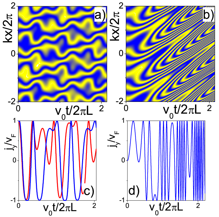
Figure 4: (Color online) Contour plot of $j_{y}(x,t)$ for the traveling wave potential (29), away from the resonance of matching velocities ($v_{\mbox{\tiny F}}/v_{0}=2.35$) a), cf. eq. (30) and at the resonance ($v_{\mbox{\tiny F}}/v_{0}=1$) b), cf. eq. (31). Bright (yellow): $j_{y}>0$, dark (blue): $j_{y}<0$. Throughout Fig. 4 we use parameters $kL=1.27$ and $W_{0}L/v_{0}=1.75$. Figures c) and d) display the time dependence of $j_{y}(x_{0},t)$ at fixed $x_{0}=L$ according to eq. (30): periodic oscillations (blue) are seen in the commensurate case, $v_{\mbox{\tiny F}}/v_{0}=2$, and aperiodic oscillations (red) when $v_{\mbox{\tiny F}}/v_{0}=2.35$. The resonant case $v_{\mbox{\tiny F}}/v_{0}=1$ is shown in d): according to eq. (31) the effective frequency of the oscillations now increases with time.

5 Conclusions

Using the exact solution of the Dirac equation for electrons in graphene moving perpendicular to a scalar potential barrier $W(x,t)$, we calculate the current component $j_{y}$ parallel to the barrier. In valley polarized situations for packets containing both, left and right moving waves, this current is nonzero despite of the vanishing incident momentum $p_{y}$. Its variance remains nonzero even without valley polarization. The here predicted current in graphene strikingly resembles the Josephson current of coupled superconductors and we find solutions that resemble Shapiro steps. Both, temporal and spatial Shapiro steps have been established, exhibiting nonzero mean current when averaged w.r.t. time or space. For time oscillating graphene superlattices and for traveling wave potentials, resonances were predicted due to spatio-temporal matching which can strongly amplify Josephson-like currents in graphene and, at large driving amplitudes, can generate a broad range of dense frequency components in the spectrum of $j_{y}(x_{0},t)$ at a given $x_{0}$. A resemblence to the ac-Josephson effect can arise.

- (1) K.S. Novoselov, A.K. Geim, S.V. Morozov, D. Jiang, M.I. Katsnelson, I.V. Grigorieva, S.V. Dubonos, A.A. Firsov, Nature 438, (2005) 197.
- (2) A.H. Castro Neto, F. Guinea, N.M.R. Peres, K.S. Novoselov, A.K. Geim, Rev. Mod. Phys. 81, (2009) 109.
- (3) M.I. Katsnelson, K.S. Novoselov, A.K. Geim, Nature Phys. 2, (2006) 620.
- (4) N. Stander, B. Huard, D. Goldhaber-Gordon, Phys. Rev. Lett. 102, (2009) 026807; A.F. Young, P. Kim, Nature Phys. 5, (2009) 222; S.-G. Nam, D.-K. Ki, J.W. Park, Y. Kim, J.S. Kim, H.-J. Lee, Nanotechnology 22, (2011) 415203.
- (5) C.X. Bai, X.D. Zhang, Phys. Rev. B 76, (2007) 075430; C.H. Park, L. Yang, Y.W. Son, M.L. Cohen, S.G. Louie, Nature Physics 4, (2008) 213; C.H. Park, L. Yang, Y.W. Son, M.L. Cohen, S.G. Louie, Phys. Rev. Lett. 101, (2008) 126804; M. Barbier, P. Vasilopoulos, F.M. Peeters, Phys. Rev. B 81, (2010) 075438; L.Z. Tan, C.H. Park, S.G. Louie, Phys. Rev. B 81, (2010) 195426.
- (6) Y.P. Bliokh, V. Freilikher, S. Savel’ev, F. Nori, Phys. Rev. B 79, (2009) 075123.
- (7) V.V. Cheianov, V. Fal’ko, B.L. Altshuler, Science 315, (2007) 1252; V.A. Yampol’skii, S. Savel’ev, F. Nori, New J. Phys. 10, (2008) 053024.
- (8) M. Barbier, P. Vasilopoulos, F.M. Peeters, Phys. Rev. B 80, (2009) 205415.
- (9) H.L. Calvo, H.M. Pastawski, S. Roche, L.E.F. Foa Torres, Appl. Phys. Lett. 98, (2011) 232103.
- (10) S.E. Savel’ev, A.S. Alexandrov, Phys. Rev. B 84, (2011) 035428.
- (11) M.V. Fistul, K.B. Efetov, Phys. Rev. Lett. 98, (2007) 256803.
- (12) H.-Y. Chiu, V. Perebeinos, Y.-M. Lin, P. Avouris, Nano Lett. 10, (2010) 4634; M.Y. Han, B. Özyilmaz, Y. Zhang, P. Kim, Phys. Rev. Lett. 98, (2007) 206805; B. Huard, J.A. Sulpizio, N. Stander, K. Todd, B. Yang, D. Goldhaber-Gordon, Phys. Rev. Lett. 98, (2007) 236803; B. Özyilmaz, P. Jarillo-Herrero, D. Efetov, D.A. Abanin, L.S. Levitov, P. Kim, Phys. Rev. Lett. 99, (2007) 166804; J.R. Williams, L. DiCarlo, C.M. Marcus, Science 317, (2007) 638.
- (13) T.K. Ghosh, A. De Martino, W. Häusler, L. Dell’Anna, R. Egger, Phys. Rev. B 77, (2008) 081404(R); W. Häusler, A. De Martino, T.K. Ghosh, R. Egger, Phys. Rev. B 78, (2008) 165402; W. Häusler, R. Egger, Phys. Rev. B 80, (2009) 161402(R); E. Grichuk, E. Manykin, Eur. Phys. J. B 86, (2013) 210.
- (14) S.E. Savel’ev, W. Häusler, P. Hänggi, Phys. Rev. Lett. 109, (2012) 226602.
- (15) J. Schliemann, Phys. Rev. B 75, (2007) 045304.
- (16) C.L. Kane, E.J. Mele, Phys. Rev. Lett. 95, (2005) 226801.
- (17) C.W.J. Beenakker, Rev. Mod. Phys. 80, (2008) 1337.
- (18) A. Rycerz, J. Tworzydlo, C.W.J. Beenakker, Nature Physics 3, (2007) 172.
- (19) S.A. Wolf, D.D. Awschalom, R.A. Buhrman, J.M. Daughton, S. von Molnár, M.L. Roukes, A.Y. Chtchelkanova, D.M. Treger, Science 294, (2001) 1488.
- (20) A.R. Akhmerov, J.H. Bardarson, A. Rycerz, C.W.J. Beenakker, Phys. Rev. B 77, (2008) 205416.
- (21) J.M. Pereira, F.M. Peeters, R.N. Costa Filho, G.A. Farias, J. Phys.: Condens. Matter 21, (2009) 045301.
- (22) J.L. Garcia-Pomar, A. Cortijo, M. Nieto-Vesperinas, Phys. Rev. Lett. 100, (2008) 236801.
- (23) A. Hill, A. Sinner, K. Ziegler, New J. Phys. 13, (2011) 035023.
- (24) T. Ando, T. Nakanishi, R. Saito, J. Phys. Soc. Jpn. 67, (1998) 2857.
- (25) E.B. Sonin, Phys. Rev. B 79, (2009) 195438.
- (26) V.V. Cheianov, V.I. Fal’ko, Phys. Rev. B 74, (2006) 041403(R).
- (27) P.G. Silvestrov, K.B. Efetov, Phys. Rev. Lett. 98, (2007) 016802.
- (28) S.V. Syzranov, M.V. Fistul, K.B. Efetov, Phys. Rev. B 78, (2008) 045407.
- (29) B. Trauzettel, Ya.M. Blanter, A.F. Morpurgo, Phys. Rev. B 75, (2007) 035305.
- (30) D. Solomon, Can. J. Phys. 88, (2010) 137.
- (31) R. Courant and D. Hilbert, Methods of Mathematical Physics (Wiley-Interscience, 1962) Volume II.
- (32) M. Tinkham, Introduction to Superconductivity (Dover Publications Inc., 2004).
- (33) S. Savel’ev, A.L. Rakhmanov, F. Nori, Phys. Rev. E 72, (2005) 056136; S. Savel’ev, A.M. Zagoskin, A.L. Rakhmanov, A.N. Omelyanchouk, Z. Washington, F. Nori, Phys. Rev. A 85, (2012) 013811.
- (34) H. Raether, Surface Plasmons (Springer, New York, 1988).