Drawing Graphs with Vertices at Specified Positions and Crossings at Large Angles

Abstract

Point-set embeddings and large-angle crossings are two areas of graph drawing that independently have received a lot of attention in the past few years. In this paper, we consider problems in the intersection of these two areas. Given the point-set-embedding scenario, we are interested in how much we gain in terms of computational complexity, curve complexity, and generality if we allow large-angle crossings as compared to the planar case.

We investigate two drawing styles where only bends or both bends and edges must be drawn on an underlying grid. We present various results for drawings with one, two, and three bends per edge.

1 Introduction

In point-set-embeddability problems one is given not just a graph that is to be drawn, but also a set of points in the plane that specify where the vertices of the graph can be placed. The problem class was introduced by Gritzmann et al. [8] twenty years ago. They showed that any $n$-vertex outerplanar graph can be embedded on any set of $n$ points in the plane (in general position) such that edges are represented by straight-line segments connecting the respective points and no two edge representations cross. Later on, the point-set-embeddability question was also raised for other drawing styles, for example, by Pach and Wenger [13] and by Kaufmann and Wiese [11] for drawings with polygonal edges, so-called polyline drawings. In these and most other works, however, planarity of the output drawing was an essential requirement.

Recent experiments on the readability of drawings [9] showed that polyline drawings with angles at edge crossings close to $90^{\circ}$ and a small number of bends per edge are just as readable as planar drawings. Motivated by these findings, Didimo et al. [4] recently defined RAC drawings where pairs of crossing edges must form a right angle and, more generally, $\alpha$AC drawings (for $\alpha\in(0,90^{\circ}]$) where the crossing angle must be at least $\alpha$. As usual, edges may not overlap and may not go through vertices.

In this paper, we investigate the intersection of the two areas, point-set embeddability (PSE) and RAC/$\alpha$AC. Specifically, we consider the following problems.

Problems RAC PSE and $\alpha$AC PSE. Given an $n$-vertex graph $G=(V,E)$ and a set $S$ of $n$ points in the plane, determine whether there exists a bijection $\mu$ between $V$ and $S$, and a polyline drawing of $G$ so that each vertex $v$ is mapped to $\mu(v)$ and the drawing is RAC (or $\alpha$AC). If such a drawing exists and the largest number of bends per edge in the drawing is $b$, we say that $G$ admits a RAC_b (or an $\alpha$AC_b) embedding on $S$.

If we insist on straight-line edges, the drawing is completely determined once we have fixed a bijection between vertex and point set. If we allow bends, however, PSE is also interesting with mapping, that is, if we are given a bijection $\mu$ between vertex and point set. We call an embedding using $\mu$ as the mapping $\mu$-respecting. The maximum number of bends over all edges in a polyline drawing is the curve complexity of the drawing.

We now list three results that motivate the study of RAC and $\alpha$AC point-set embeddings—even for planar graphs.

• Rendl and Woeginger [16] have already considered a special case of the question we investigate in this paper, that is, the interplay between planarity and RAC in PSE. They showed that, given a set $S$ of $n$ points in the plane, one can test in $O(n\log n)$ time whether a perfect matching admits a RAC₀ embedding on $S$. They required that edges are drawn as axis-aligned line segments. They also showed that if one additionally insists on planarity, the problem becomes NP-hard.

• Pach and Wenger [13] showed for the polyline drawing scenario with mapping that, if one insists on planarity, $\Omega(n)$ bends per edge are sometimes necessary even for the class of paths and for points in convex position.

• Cabello [2] proved that deciding whether a graph admits a planar straight-line embedding on a given point set is NP-hard even for $2$-outerplanar graphs.

In this paper, we concentrate on RAC PSE. In order to measure the size of our drawings, we assume that the given point set $S$ lies on a grid of size $n\times n$ where $n=|S|$. We further assume that the points in $S$ are in general position, that is, no two points lie on the same horizontal or vertical line. We call $S$ an $n\times n$ grid point set. We require that, in our output drawings, bends lie on grid points. We concentrate on two variants of the problem. We either restrict the edges, which are drawn as polygonal lines, to grid lines or we don’t. We refer to the restricted version of the problem as restricted RAC/$\alpha$AC PSE. We treat the restricted version in Section 2 and the unrestricted version in Section 3. The graphs we study are always undirected.

Our results concerning restricted RAC and $\alpha$AC PSE are as follows.

• Every $n$-vertex binary tree admits a restricted RAC₁ embedding on any $n\times n$ grid point set (Theorem 2.1). This is not known for the planar case—see our list of open problems in Section 4. We slightly extend this result to graphs of maximum degree 3 that arise when replacing the vertices of a binary tree by cycles. In the case of a single cycle, the statement even holds if the mapping is prescribed. This is not true in the planar case: take the 4-vertex cycle and the four points $(2,2),(4,4),(1,1),(3,3)$, in this order.

• Given a graph, a point set on the grid, and a mapping $\mu$, we can test in linear time whether the graph admits a $\mu$-respecting restricted RAC₁ point-set embedding (Theorem 2.3). The same simple 2-SAT based test works in the planar case but of course fails more often.

• Every $n$-vertex graph of maximum degree 3 admits a restricted RAC₂ embedding on any $n\times n$ grid point set even if the mapping is prescribed (Theorem 2.4). Given a matching with $n$ vertices, a set of $n$ points on the $y$-axis, and a mapping $\mu$, we can compute, in $O(n^{2})$ time, a $\mu$-respecting restricted RAC₂ embedding of minimum area (to the right of the $y$-axis, see Theorem 2.5).

Concerning unrestricted RAC and $\alpha$AC PSE, we show the following results which all hold even if the mapping is prescribed.

• Every graph with $n$ vertices and $m$ edges admits a RAC₃ embedding on any $n\times n$ grid point set within area $O\!\left((n+m)^{2}\right)$ (Theorem 3.1). To RAC draw arbitrary graphs, curve complexity 3 is needed—even without PSE [1]. In the planar case (with mapping), the curve complexity for PSE is $\Omega(n)$ [13].

• For any $\varepsilon>0$, we get a $(\pi/2-\varepsilon)$AC₂ drawing within area $O(nm)$ (Theorem 3.2). On a grid refined by a factor of $O(1/\varepsilon^{2})$, we get a $(\pi/2-\varepsilon)$AC₁ drawing within area $O(n^{2})$ (Theorem 3.3), which is optimal [6]. In the planar case, it is NP-hard to decide the existence of a 1-bend point-set embedding—both with [7] and without [11] prescribed mapping.

Related work.

Besides the above-mentioned work of Rendl and Woeginger [16], the study of PSE has primarily focussed on the planar case, in connection with the drawing conventions straight-line and polyline. A special case of the polyline drawings are Manhattan-geodesic drawings which require that the edges are drawn as monotone chains of axis-parallel line segments. This convention was recently introduced by Katz et al. [10]. They proved that Manhattan-geodesic PSE is NP-hard (even for subdivisions of cubic graphs). On the other hand, they provided an $O(n\log n)$ decision algorithm for the $n$-vertex cycle. They also showed that Manhattan-geodesic PSE with mapping is NP-hard even for perfect matchings—if edges are restricted to the grid.

Although RAC and $\alpha$AC drawings have been introduced very recently, there is already a large body of literature on the problem. Regarding the area of RAC drawings, Didimo et al. [4] proved that an unrestricted RAC₃ drawing of an $n$-vertex graph uses area $\Omega(n^{2})\cap O(m^{2})$. Di Giacomo et al. [6] showed that, for RAC₄ drawings, area $O(n^{3})$ suffices and that, for any $\varepsilon>0$, every $n$-vertex graph admits a $(\pi/2-\varepsilon)$AC₁ drawing within area $\Theta(n^{2})$. Our results for RAC₃ and AC₁ drawings (in Theorems 3.1 and 3.3) match the ones cited here, in spite of the fact that vertex positions are prescribed in our case.

2 Restricted RAC Point-Set Embeddings

In this section, we study restricted RAC point-set embeddings. It is clear that only graphs with maximum degree $4$ may admit a restricted RAC embedding on a point set. We start with the study of RAC₁ drawings.

2.1 Restricted RAC₁ point-set embeddings

The following result was independently achieved by Di Giacomo et al. [3].

Theorem 2.1

Every binary tree has a restricted RAC₁ embedding on every $n\times n$ grid point set.

Proof

Let $S$ be an $n\times n$ grid point set, let $T$ be a binary tree rooted at an arbitrary vertex $r$, and let $v_{1},\dots,v_{n}$ be a numbering of the vertices of $T$ given by a breadth-first-search traversal starting from $r$, i.e., $v_{1}=r$. For $i=1,\dots,n$, let $T_{i}$ be the subtree of $T$ rooted at vertex $v_{i}$.

Let $p_{1}$ be the point in $S$ such that the vertical line $\ell_{1}$ through $p_{1}$ splits $S_{1}=S$ according to $T_{1}=T$, that is, we split $S_{1}$ into a set $S_{2}$ of $|T_{2}|$ points on its left and a set $S_{3}$ of $|T_{3}|$ points on its right; see Fig. LABEL:sub@sfg:partition. Then we recursively pick points $p_{2}$ and $p_{3}$ and lines $\ell_{2}$ and $\ell_{3}$ that partition $S_{2}$ and $S_{3}$ according to $|T_{2}|$ and $|T_{3}|$. We continue until we arrive at the leaves of $T$. This process determines points $p_{1},\dots,p_{n}$ and lines $\ell_{1},\dots,\ell_{n}$ such that for $i=1,\dots,n$ point $p_{i}$ lies on $\ell_{i}$. We simply map vertex $v_{i}$ to point $p_{i}$ for $i=1,\dots,n$.

Consider an index $i\in\{1,\dots,n\}$. Our mapping makes sure that one subtree of $T_{i}$ is drawn on the left of $\ell_{i}$ and the other on the right of $\ell_{i}$. Let $v_{j}$ and $v_{j+1}$ be the children of $v_{i}$. We draw the edges $(v_{i},v_{j})$ and $(v_{i},v_{j+1})$ such that their horizontal segments are both incident to $v_{i}$, see Fig. LABEL:sub@sfg:edgedrawing.

The resulting drawing is clearly a RAC drawing since all edges are restricted to the grid. Since $S$ is in general position, no two edges can overlap except if they are incident to the same vertex. If we direct the edges of $T$ away from the root, then, by our drawing rule, in any vertex $v_{i}$ of $T$ the incoming edge arrives in $p_{i}$ with a vertical segment and the outgoing edges leave $p_{i}$ with horizontal segments in opposite directions.

We can, of course, also find a restricted RAC₁ embedding for paths as special binary trees. Actually, we can embed every $n$-vertex path or cycle on any $n\times n$ grid point set, even with mapping: we simply leave each point horizontally and enter the next one vertically in the order prescribed by the mapping.

It would, of course, be nice to generalize these embeddability results for binary trees and cycles (without given mapping) to larger classes of graphs, e.g., outerplanar graphs of maximum degree 3. This seems, however, to be quite difficult. A class of graphs that we can embed are maxdeg-3 cactus graphs that are constructed from binary trees by replacing vertices by cycles.

We can embed graphs of this type on any $n\times n$ grid point set by adjusting the embedding algorithm for binary trees. The basic idea is to treat each cycle similarly to a single tree vertex. We do this by reserving the adequate number of consecutive columns for the vertices of the cycle in the middle of the drawing area for the current subtree. We connect the cycle to the left subtree by leaving the leftmost reserved point to the left. We deal with the right subtree symmetrically. One of the points reserved for the cycle—say, $z$—must be connected to the parent vertex (or cycle). The difficulty is to make a cycle from the reserved points in such a way that $z$ can be entered vertically from its parent, which has been embedded before. This is possible but the proof is technical, and, hence, left for the appendix. Summing up, we get the following result.

Theorem 2.2

Let $G$ be an $n$-vertex graph of maximum degree 3 that arises when replacing the vertices of a binary tree by cycles and let $S$ be an $n\times n$ grid point set. Then $G$ admits a restricted RAC₁ embedding on $S$.

In the proofs of the previous theorems we exploited the fact that we could choose the vertex–point mapping as needed. Figure 2 shows a 6-vertex binary tree that does not have a restricted RAC₁ drawing on the given point set if the vertex–point mapping is fixed as indicated by the edges. Hence, we turn to the corresponding decision problem. We characterize situations when a restricted RAC₁ point-set embedding with mapping exists.

 

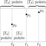
(a) Partition of the point set

  

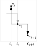
(b) Drawing of the edges

Figure 1: Illustrations for the proof of Theorem 2.1.

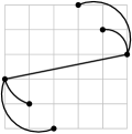
Figure 2: A binary tree without restricted RAC₁ drawing.

Theorem 2.3

Let $G$ be an $n$-vertex graph of maximum degree $4$, let $S$ be an $n\times n$ grid point set, and let $\mu$ be a vertex–point mapping. We can test in $O(n)$ time whether $G$ admits a $\mu$-respecting restricted RAC₁ embedding on $S$ and, if yes, construct such an embedding within the same time bound.

Proof

We use a 2-SAT encoding to solve the problem. A similar approach was used by Raghavan et al. [15] to deal with the planar case. We associate each edge $uv$ of $G$ with a Boolean variable $x_{uv}$. The two possible drawings of edge $uv$ correspond to the two literals $x_{uv}$ and $\neg x_{uv}$. Due to the fact that $S$ is in general position, only drawings of edges incident to the same vertex can possibly overlap.

Now we construct a 2-SAT formula $\phi$ as follows. Consider a pair of drawings of edges $uv$ and $uw$ that overlap. Assume that $x_{uv}$ and $\neg x_{vw}$ are the literals corresponding to the two edge drawings. Then we add the clause $\neg(x_{uv}\wedge\neg x_{uw})=\neg x_{uv}\vee x_{uw}$ to $\phi$.

It is clear that $\phi$ is satisfiable if and only if $G$ has a $\mu$-respecting RAC₁ embedding on $S$ without overlapping edges. Recall that the maximum degree of $G$ is 4. Hence, $\phi$ contains at most $n\cdot\binom{4}{2}\cdot 4$ clauses. Since the satisfiability of a 2-SAT formula can be decided in time linear in the number of clauses [5], the testing can be done in $O(n)$ time.

2.2 Restricted RAC₂ point-set embeddings

As in the previous subsection, it is clear that only graphs of maximum degree 4 can be drawn with the grid restriction. Consider, for a moment, a specialized restricted RAC₂ drawing convention that requires the first and the last (of the three) segments of an edge to go in the same direction—a bracket drawing. If we do not restrict the drawing area, then the problem of bracket embedding a graph $G$ on an $n\times n$ grid point set is equivalent to $4$-edge coloring $G$. The idea is that the four colors encode the direction of the first and last edge segment (going up, down, left, or right) and that the second edge segment is drawn sufficiently far away. The edge coloring makes sure that no two edges incident to the same vertex overlap. It is known that any graph of maximum degree 3 is $4$-edge colorable and that such a coloring can be found in linear time [17]. Let us summarize.

Theorem 2.4

Every graph $G$ of maximum degree 3 admits a restricted RAC₂ embedding on any $n\times n$ grid point set with any vertex–point mapping.

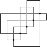
Figure 18: Restricted RAC₂ drawing of $K_{5}$ on a diagonal point set.

Note that there are graphs of maximum degree 4 that do not admit a $4$-edge coloring, but do admit a restricted RAC₂ embedding at least for some grid point sets (see Figure 18 in the appendix for such an embedding of $K_{5}$).

Now we turn to the problem of minimizing the drawing area. Observe that there are examples of a graph $G$, a grid point set $S$, and a mapping $\mu$ such that $G$ does not admit a restricted RAC₂ point-set embedding on $S$ with mapping $\mu$ if we insist that the drawing lies within the bounding box of $S$, see Fig. 3.

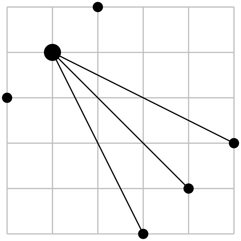
Figure 3: Counterexample.

We conjecture that restricted RAC₂ PSE is NP-hard. Therefore, we consider the special case where $S$ is one-dimensional. More precisely, we are looking for a one-page RAC₂ book embedding with given mapping. Recall that, generally, a $k$-page book embedding asks for a mapping of the vertices to points on a line, the spine of the book, and a mapping of the edges to the pages of the book (that is, half-planes incident to the spine) such that, for each page, the edges on that page can be drawn without crossings.

Clearly, in this setting, each vertex can only have degree 1, hence the given graph must be a (perfect) matching. Given these restrictions, we can minimize the area of the drawing.

Theorem 2.5

Let $S$ be a set of $n$ points on the $y$-axis, let $G$ be a matching consisting of $n/2$ edges, and let $\mu$ be a vertex–point mapping. A minimum-area $\mu$-respecting restricted RAC₂ drawing of $G$ to the right of the $y$-axis can be computed in $O(n^{2})$ time.

Proof

If $S$ contains pairs of neighboring points that correspond to edges of the given matching, we connect each of them by a (vertical) straight-line segment. To draw any of the remaining edges of the matching in a restricted RAC₂ fashion, we must connect its endpoints by two horizontal segments leaving the $y$-axis to the right and a vertical segment that joins the horizontal segments. As $G$ is a matching, only vertical segments can overlap. In order to minimize the drawing area, we, thus, have to minimize the number of vertical lines, the layers, needed to draw the vertical segments of all edges without overlap.

Let $G^{\prime}=(V^{\prime},E^{\prime})$ with $V^{\prime}=E$ and an edge connecting each pair of edges of $G$ that cannot use the same layer. Clearly, assigning the edges of $G$ to the minimum number of layers is the same as coloring the vertices of $G^{\prime}$ with the minimum number $\chi^{\prime}$ of colors.

Graph $G^{\prime}$ is an interval graph: for edge $uv$ of $G$—a vertex of $G^{\prime}$—the interval is $[\mu(u),\mu(v)]$. Hence, a coloring of $G^{\prime}$ using $\chi^{\prime}$ colors can be computed in $O(|V^{\prime}|+|E^{\prime}|)=O(n^{2})$ time [12]. This coloring yields an assignment of the edges to the minimum number of layers, which in turn corresponds to a minimum-area restricted RAC₂ drawing: we simply use the first $\chi^{\prime}$ vertical grid lines immediately to the right of the $y$-axis for the layers of the vertical edge segments.

If we are not given a prescribed mapping, then the problem becomes easy for all graphs of maximum degree 2. We simply draw the connected components of $G$, which are paths or cycles, one after the other using the points in $S$ from top to bottom. This can be done using only the $y$-axis for paths and using only one column right of the $y$-axis for cycles.

If we abandon the restriction to draw edges on the grid and relax the constraint on the crossing angle, we can find, for any graph, an $\alpha$AC₂ embedding on any point set on the $y$-axis with an arbitrary mapping, see the comment after the proof of Theorem 3.2.

3 Unrestricted RAC and $\alpha$AC Point-Set Embeddings

Didimo et al. [4] have shown that any graph with $n$ vertices and $m$ edges admits a RAC₃-drawing within area $O(m^{2})$. Their proof uses an algorithm of Papakostas and Tollis [14] for drawing graphs such that each vertex is represented by an axis-aligned rectangle and each edge by an L-shape, that is, an axis-aligned 1-bend polyline. Didimo et al. turn such a drawing into a RAC₃-drawing by replacing each rectangle with a point. In order to make the edges terminate at these points, they add at most two bends per edge. We now show how to compute a RAC₃-drawing of the same size (assuming $n\in O(m)$)—although we are restricted to the given point set.

Note that curve complexity 3 is actually necessary for RAC drawing arbitrary graphs—even without a prescribed point set: Arikushi et al. [1] showed that RAC₂ drawings only exist for graphs with a linear number of edges.

Theorem 3.1

Let $G$ be a graph with $n$ vertices and $m$ edges and let $S$ be an $n\times n$ grid point set. Then $G$ admits a RAC₃-drawing on $S$ (with or without given vertex–point mapping) within area $O\left((n+m)^{2}\right)$.

Proof

If the vertex–point mapping $\mu$ is not given, let $\mu$ be an arbitrary mapping. Let $v_{1},\ldots,v_{n}$ be an ordering of $V$ so that $p_{i}:=\mu(v_{i})$ has $x$-coordinate $i$. We construct a RAC₃-drawing as follows. Each edge has—after insertion of “virtual” bends—exactly three bends and four straight-line segments. We ensure that intersections involve only the “middle” segments of edges, and that these middle segments have only slope $+1$ or $-1$.

For an edge $uv$, we call the bend directly connected to $u$ a $u$-bend, the bend directly connected to $v$ a $v$-bend, and the remaining bend the middle bend. We start constructing the drawing by placing the $v$-bends for each vertex $v$, starting with $v_{n}$. We set the $y$-coordinate $y_{n}$ of the first $v_{n}$-bend to 0. Then, for $i=n,n-1,\dots,1$, observe that there are exactly $\deg v_{i}$ many $v_{i}$-bends, which we place in column $i+1$ starting at $y$-coordinate $y_{i}$ below the $n\times n$ grid using positions $\{(i+1,y_{i}),(i+1,y_{i}-2),(i+1,y_{i}-4),\ldots,(i+1,y_{i}-2\cdot(\deg v_{i}-1)\}$, see Figure 5. We connect each vertex with its associated bends without introducing any intersection since we stay inside the area between columns $i$ and $i+1$. We set $y_{i-1}=y_{i}-2\cdot(\deg v_{i}-1)-3$. If $v_{i}$ has degree 0, we do not place bends but set $y_{j-1}=y_{j}-3$ to avoid overlaps and crossings. Then we continue with $v_{i-1}$.

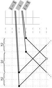
Figure 4: Construction of a RAC₃ drawing.

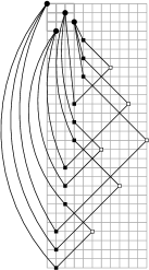
Figure 5: RAC₃-drawing of $K_{4}$ as in the proof of Theorem 3.1. For the sake of clarity, we replaced some straight-line segments by circular arcs.

Since we place the bends from right to left and from top to bottom by moving our “pointer” by $L_{1}$- (or Manhattan) distances 2 or 4, each pair of these bends has even Manhattan distance. To draw an edge $uv$, we first select a “free” $u$-bend position and a free $v$-bend position. For the two middle segments, we use slopes $+1$ and $-1$ such that the middle bend is to the right of the $u$- and $v$-bend. Since $u$- and $v$-bend have even Manhattan distance, the middle bend has integer coordinates.

Let $u$ and $v$ be two vertices with $u$-bend $b_{u}$ and $v$-bend $b_{v}$, respectively. The segments $\overline{ub_{u}}$ and $\overline{vb_{v}}$ cannot intersect; we want to see that the middle segment starting at $b_{u}$ also cannot intersect $\overline{vb_{v}}$. Such an intersection can only occur if $u$ lies to the left of $v$.By our construction, $b_{v}$ lies, in this case, above $b_{u}$ with a $y$-distance that is greater than their $x$-distance. As all middle segments have a slope of at most $+1$, $b_{v}$ lies above the relevant middle segment, which can, hence, not intersect $\overline{vb_{v}}$.

It remains to show the space limitation. Clearly, the drawing of any edge requires not more horizontal than vertical space. On the other hand, for any vertex $v$, we need at most $2\cdot\deg v+3$ rows below the grid, resulting in a total vertical space requirement of $O(n+m)$. This completes the proof.

In the remainder of this section we focus on $\alpha$AC point-set embeddings. We show that both area and curve complexity can be significantly improved if we soften the restriction on the crossing angles. Our results hold for both scenarios, with and without vertex–point mapping.

Theorem 3.2

Let $G$ be a graph with $n$ vertices and $m$ edges, let $S$ be a $n\times n$ grid point set, and let $0<\varepsilon<\frac{\pi}{2}$. Then $G$ admits a $(\frac{\pi}{2}-\varepsilon)$AC₂ embedding on $S$ (with or without given vertex–point mapping) within area $O(n(m+\cot\varepsilon))=O(n(m+1/\varepsilon^{2}))$.

Proof

If the vertex–point mapping $\mu$ is not given, let $\mu$ be arbitrary. Let $v_{1},\dots,v_{n}$ be an ordering of $V$ so that $p_{i}:=\mu(v_{i})$ has $x$-coordinate $i$. Each edge $e=uv$ has exactly two bends, a $u$-bend and a $v$-bend (with the obvious meanings). For $i=1,\dots,n$, we place all $v_{i}$-bends in column $i+1$. We make all middle segments of edges horizontal. Thus, the bends for an edge $e=v_{i}v_{j}$ are at positions $(i+1,y)$ and $(j+1,y)$ in some row $y<0$ below the original grid, see Figure 7. By using a dedicated row for each edge, we achieve that no two middle segments intersect. By construction, no two first or last edge segments intersect. Hence, crossings occur only between the horizontal middle segments and first or last segments. By making the $y$-coordinates of the middle segments small enough, we will achieve that all crossing angles are at least $\pi/2-\varepsilon$.

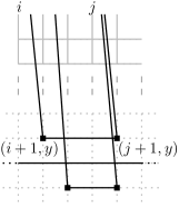
Figure 6: Constructing a 2-bend drawing with large crossing angles.

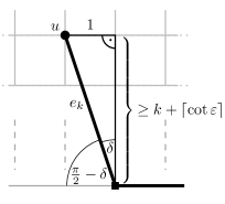
Figure 7: Angles in the 2-bend drawing.

Let $\{e_{1},\ldots,e_{m}\}$ be the set of edges of $G$, and let $uv:=e_{k}$ be one of these edges. We set the $y$-coordinates of the middle segment of $e_{k}$ to $-k-\lceil\cot\varepsilon\rceil$. Let $e_{k^{\prime}}$ be an edge whose horizontal segment intersects the first segment of $e_{k}$. The crossing angle is $\pi/2-\delta$, where $\delta$ is the angle between the vertical line through the $u$-bend and the first segment of $uv$, see Figure 7. We have $\delta\leq\operatorname{arccot}(k+\lceil\cot\varepsilon\rceil)\leq\varepsilon$. Thus, the crossing angle is at least $\pi/2-\varepsilon$. Note that $\cot\varepsilon\in O(1/\varepsilon^{2})$.

We used only the fact that no two points lie in the same column. Hence, the statement of the theorem does not change if we allow the points to lie on a single horizontal (or, by rotation, vertical) line as in Section 2.2.

In Theorem 3.2, we required the bends to lie on points of the given grid. The following result shows that we need only one bend per edge if we allow the bends to lie on points of a refined grid. For fixed $\epsilon>0$, our new drawings need less area than those of Theorem 3.2; even in terms of the refined grid.

Theorem 3.3

Let $G$ be a graph with $n$ vertices, let $S$ be an $n\times n$ grid point set, and let $0<\varepsilon<\frac{\pi}{2}$. Then $G$ admits a $(\frac{\pi}{2}-\varepsilon)$AC₁ embedding on $S$ (with or without given vertex–point mapping) on a grid that is finer than the original grid by a factor of $\lambda\in O(\cot\varepsilon)=O(1/\varepsilon^{2})$.

Proof

If the mapping $\mu$ is not given, let $\mu$ be an arbitrary mapping. The idea of our construction is as follows. For each edge, we first choose one of the two possible drawings on the grid lines with one bend. This gives us a drawing of the graph with many overlaps of edges. Then, we slightly twist each edge such that its horizontal segment becomes almost horizontal, meaning it gets a negative slope close to 0. At the same time, we make the vertical segment almost vertical, meaning it gets a very large positive slope, see Figure 9.

As we want all bends to be on grid points, we first refine the grid by an integral factor of $\lambda=\lceil 1+\cot\varepsilon\rceil$. We do this by inserting, at equal distances, $\lambda-1$ new rows or columns between two consecutive grid rows or columns, respectively. Now, a point $s=(a,b)\in S$ lies at $(\lambda a,\lambda b)$ w.r.t. the new $\lambda n\times\lambda n$ grid.

Let $e$ be an edge and let $(e_{x},e_{y})$ be the original position of the bend of $e$ w.r.t. the new grid. We choose the new position of the bend to be the unique grid point diagonally next to $(e_{x},e_{y})$ such that the horizontal and vertical segments of $e$ become almost horizontal and almost vertical, respectively. If we apply this construction to all edges, we get a drawing in which none of the almost horizontal and almost vertical segments belonging to some vertex $v$ can overlap. Moreover, two almost horizontal or two almost vertical segments belonging to different vertices neither overlap nor intersect due to $S$ being in general position. Thus, each crossing involves an almost horizontal and an almost vertical segment.

Let $e_{1}$ and $e_{2}$ be two crossing edges such that the almost horizontal segment involved in the crossing belongs to $e_{1}$. We can assume that the smaller angle of the crossing occurs to the top left of the crossing; the other case is symmetric by a rotation of the plane. Let $\delta^{-}$ be the angle formed by the almost horizontal segment of $e_{1}$ and a horizontal line, and let $\delta^{+}$ be the angle formed by the almost vertical segment of $e_{1}$ and a vertical line, see Figure 9. Then the crossing angle of $e_{1}$ and $e_{2}$ is $\alpha=\pi/2-\delta^{-}+\delta^{+}\geq\pi/2-\delta^{-}$. For $\delta^{-}$ to be maximal, the horizontal length $l$ of the almost horizontal segment has to be minimal. As this length cannot be less than $\lambda-1$, we get $\delta^{+}\leq\operatorname{arccot}(\lambda-1)\leq\varepsilon$. Hence, the crossing angle $\alpha$ is at least $\pi/2-\varepsilon$.

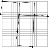
Figure 8: Drawing of $K_{4}$ on a grid refined by factor $\lambda=8$.

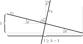
Figure 9: Angles in the 2-bend-drawing.

Note that we leave the original grid by at most one row or column of the refined grid in each direction. Hence, the area requirement is $O((n\cdot\cot\varepsilon)^{2})$ in terms of the finer grid. We argue that our area bounds are quite reasonable: for a minimum crossing angle of $70^{\circ}$, the drawings provided by Theorems 3.2 and 3.3 use grids of sizes at most $n(m+3)$ and $(3n)^{2}$, respectively.

4 Open Problems

In this paper, we have opened an interesting new area: the intersection of point-set embeddability and drawings with crossings at large angles. We have done a few first steps, but we leave open a large number of questions. We start with the restricted case where vertices, bends, and edges must lie on the grid.

1. Does every $n$-node binary tree have a restricted planar 1-bend embedding on any $n\times n$ grid point set?

2. Does every $n$-node ternary tree have a restricted RAC₁ embedding on any $n\times n$ grid point set?

3. What about outerplanar graphs?

4. Can we efficiently test whether a given graph has a restricted RAC₁ embedding on a given $n\times n$ grid point set?

5. What about RAC₂?

Recall that in the unrestricted case we don’t require edges to lie on the grid.

1. Can we efficiently test whether a given graph has a RAC₂ embedding on a given $n\times n$ grid point set? If yes, can we minimize its area?

2. Di Giacomo et al. [6] have shown that any graph with $n$ vertices and $m$ edges admits a RAC₄-drawing that uses area $O(n^{3})$. Can we achieve the same in our PSE setting?

Acknowledgments. We thank Beppe Liotta for suggesting the idea behind Theorem 3.3 to us.

Appendix

Theorem 0..2

Let $G$ be an $n$-vertex graph of maximum degree 3 that arises when replacing the vertices of a binary tree by cycles and let $S$ be an $n\times n$ grid point set. Then $G$ admits a restricted RAC₁ embedding on $S$.

Proof

We adjust the embedding algorithm for binary trees to work with the new graph class. The basic idea is to treat each cycle similar to a single vertex of a binary tree. We do this by reserving the adequate number of consecutive columns for the nodes of the cycle in the middle of the drawing area for the current subtree when splitting into the drawing areas for the subtrees. The subtrees are connected to the cycle by leaving one point to the right, and one point to the left, respectively. The most difficult part is to connect the reserved nodes to a cycle in such a way that the point representing the vertex that is the connector to the parent vertex (or cycle, respectively), which was embedded before, can be connected by entering the node with a vertical segment such that the connections to the left and the right are possible.

Let $C$ with $k:=|C|\geq 3$ be the cycle representing the root of the current subtree with vertices $u$ and $v$ connecting the cycle to the roots $r_{l}$ and $r_{r}$ of its left and right subtrees, respectively, and a vertex $z$ connecting $C$ to its parent $r$. Let $S^{\prime}=\left\{p_{1},\ldots,p_{k}\right\}$ be the set of points reserved for $C$ in consecutive columns ordered from left to right. The edge connecting $C$ to the left and right subtree enter the points representing $u$ and $v$ from left and right, respectively, while the edge connecting $z$ to $r$ enters $z$ from above or below, depending on the $y$-coordinate of the point chosen to represent $z$. Let $y_{r}$ be the $y$-coordinate of $r$. We analyze the different cases.

1. Vertex $z$ has a neighbor $w\neq u,v$ in $C$ and $k\geq 5$:

   Set $\mu(u)=p_{1}$ and $\mu(v)=p_{k}$. Either above or below the line $y=y_{r}$ we find two points $p,p^{\prime}\in S^{\prime}\setminus\left\{p_{1},p_{k}\right\}$. Let $p$ be the one closer to the line $y=y_{r}$. We set $\mu(p)=z,\mu(p^{\prime})=w$ and draw the edge $wz$ such that $p$ is entered vertically. Then we can complete the cycle such that each point is incident to a horizontal and a vertical segment, see Figure 11. It is easy to see that the connections to $r,r_{l}$ and $r_{r}$ can now be drawn without overlap.

   

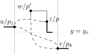
   Figure 10: Drawing of $C$ with at least 5 vertices and a neighbor $w$ of $z$.

   

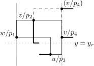
   Figure 11: Drawing of $C$ with $k=4$ and $p_{4}$ above $p_{3}$.

2. Vertex $z$ has a neighbor $w\neq u,v$ in $C$ and $k=4$:

   Let $C=\left(u,w,z,v\right)$ the other case being symmetric. If $p_{2}$ and $p_{3}$ both lie either below or above $y=y_{r}$ we can proceed as in case 1. If $p_{2}$ lies above $r$ and $p_{3}$ below we have two subcases depending on where $p_{4}$ is:

   • $p_{4}$ lies above $p_{3}$: We can draw $C$ as shown in Figure 11.

   • $p_{4}$ lies below $p_{3}$: We can draw $C$ as shown in Figure 13.

   

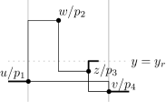
   Figure 12: Drawing of $C$ with $k=4$ and $p_{4}$ below $p_{3}$.

   

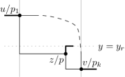
   Figure 13: Drawing of $C$ with $u,v$ as neighbors of $z$ and one point vertically between $p_{1}$ and $p_{k}$.

   If $p_{3}$ is above $r$ and $p_{2}$ below the cases are symmetric.

3. The two neighbors of $z$ are $u$ and $v$. If there is one point $p\in S^{\prime}\setminus\left\{p_{1},p_{k}\right\}$ that is vertically between $p_{1}$ and $p_{k}$, then we set $\mu(u)=p_{1},\mu(v)=p_{k}$ and $\mu(z)=p$ and draw $C$ as in Figure 13, where the second path connecting $u$ and $v$ can be drawn by having a vertical and a horizontal segment incident to each point.

   In the remaining cases, there is no such point vertically between $p_{1}$ and $p_{k}$.

   • If $k\geq 5$ we find, similar to case 1, two points $p,p^{\prime}\in S^{\prime}\setminus\left\{p_{1},p_{k}\right\}$ both below or above $r$ such that $p$ is the one closer to the line $y=y_{r}$. Again we set $\mu(z)=p$; if $p^{\prime}$ is left of $p$ we set $\mu(u)=p^{\prime}$ and $\mu(v)=p_{k}$, see Figure 15, and otherwise we symmetrically set $\mu(v)=p^{\prime}$ and $\mu(u)=p_{1}$. Now we can draw the cycle without overlap such that each point is incident to a vertical and a horizontal segment.

   • If $k=4$, we have $C=(u,z,v,w)$. If $p_{2}$ and $p_{3}$ lie both above or below $r$ we can proceed as in the previous case. Otherwise we know that both points are on different sides of $y=y_{r}$, and that $p_{1}$ and $p_{4}$ are both vertically between, below, or above $p_{2}$ and $p_{3}$. In the first case, we set $\mu(u)=p_{1},\mu(v)=p_{4},\mu(z)=p_{2}$ and $\mu(w)=p_{3}$ and create the drawing of $C$ as in Figure 15. As above and below are symmetric, the other two cases can be handled as shown in Figure 17.

     

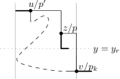
     Figure 14: Drawing of $C$ with $u,v$ as neighbors of $z$ and $k\geq 4$.

     

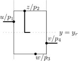
     Figure 15: Drawing of $C$ with $u,v$ as neighbors of $z$, $k=4$, and $p_{1},p_{4}$ vertically between $p_{2}$ and $p_{3}$.

   • Finally, if $k=3$, we set $\mu(u)=p_{1},\mu(v)=p_{3}$ and $\mu(z)=p_{2}$, and simply draw as shown in Figure 17.

     

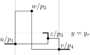
     Figure 16: Drawing of $C$ with $u,v$ as neighbors of $z$, $k=4$, and $p_{1},p_{4}$ vertically below $p_{2}$ and $p_{3}$.

     

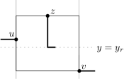
     Figure 17: Drawing of $C$ with $u,v$ as neighbors of $z$ and $k=3$.

References

- [1] K. Arikushi, R. Fulek, B. Keszegh, F. Morić, and C. Tóth. Graphs that admit right angle crossing drawings. In D. Thilikos, editor, Proc. 36th Int. Workshop Graph Theoretic Concepts Comput. Sci. (WG’10), volume 6410 of LNCS, pages 135–146. Springer-Verlag, 2010.
- [2] S. Cabello. Planar embeddability of the vertices of a graph using a fixed point set is NP-hard. J. Graph Alg. Appl., 10(2):353–366, 2006.
- [3] E. Di Giacomo, F. Frati, R. Fulek, L. Grilli, and M. Krug. Personal communication, 2011.
- [4] W. Didimo, P. Eades, and G. Liotta. Drawing graphs with right angle crossings. In F. K. Dehne, M. L. Gavrilova, J.-R. Sack, and C. D. Tóth, editors, Proc. 11th Int. Workshop Algorithms Data Struct. (WADS’09), volume 5664 of LNCS, pages 206–217. Springer-Verlag, 2009.
- [5] S. Even, A. Itai, and A. Shamir. On the complexity of timetable and multicommodity flow problems. SIAM J. Comput., 5(4):691–703, 1976.
- [6] E. D. Giacomo, W. Didimo, G. Liotta, and H. Meijer. Area, curve complexity, and crossing resolution of non-planar graph drawings. Theory Comput. Syst., pages 1–11, 2010.
- [7] X. Goaoc, J. Kratochvíl, Y. Okamoto, C.-S. Shin, A. Spillner, and A. Wolff. Untangling a planar graph. Discrete Comput. Geom., 42(4):542–569, 2009.
- [8] P. Gritzmann, B. Mohar, J. Pach, and R. Pollack. Embedding a planar triangulation with vertices at specified positions. Amer. Math. Mon., 98:165–166, 1991.
- [9] W. Huang, S.-H. Hong, and P. Eades. Effects of crossing angles. In Proc. 7th Int. IEEE Asia-Pacific Symp. Inform. Visual. (APVIS’08), pages 41–46, 2008.
- [10] B. Katz, M. Krug, I. Rutter, and A. Wolff. Manhattan-geodesic embedding of planar graphs. In D. Eppstein and E. R. Gansner, editors, Proc. 17th Int. Symp. Graph Drawing (GD’09), volume 5849 of LNCS, pages 207–218. Springer-Verlag, 2010.
- [11] M. Kaufmann and R. Wiese. Embedding vertices at points: Few bends suffice for planar graphs. J. Graph Alg. Appl., 6(1):115–129, 2002.
- [12] S. Olariu. An optimal greedy heuristic to color interval graphs. Inform. Process. Lett., 37(1):21–25, 1991.
- [13] J. Pach and R. Wenger. Embedding planar graphs at fixed vertex locations. Graphs Combin., 17(4):717–728, 2001.
- [14] A. Papakostas and I. G. Tollis. Efficient orthogonal drawings of high degree graphs. Algorithmica, 26:100–125, 2000.
- [15] R. Raghavan, J. Cohoon, and S. Sahni. Single bend wiring. J. Algorithms, 7(2):232–257, 1986.
- [16] F. Rendl and G. Woeginger. Reconstructing sets of orthogonal line segments in the plane. Discrete Math., 119:167–174, 1993.
- [17] S. Skulrattanakulchai. 4-edge-coloring graphs of maximum degree 3 in linear time. Inform. Process. Lett., 81(4):191–195, 2002.