IPMU 11-0124

UT-11-22

Isocurvature perturbations in extra radiation

Masahiro Kawasaki^a,b, Koichi Miyamoto^a, Kazunori Nakayama^c

and Toyokazu Sekiguchi^d

^aInstitute for Cosmic Ray Research, University of Tokyo, Kashiwa 277-8582, Japan
^bInstitute for the Physics and Mathematics of the Universe, University of Tokyo, Kashiwa 277-8568, Japan
^cDepartment of Physics, University of Tokyo, Bunkyo-ku, Tokyo 113-0033, Japan
^dDepartment of Physics and Astrophysics, Nagoya University, Nagoya 464-8602, Japan

Recent cosmological observations, including measurements of the CMB anisotropy and the primordial helium abundance, indicate the existence of an extra radiation component in the Universe beyond the standard three neutrino species. In this paper we explore the possibility that the extra radiation has isocurvatrue fluctuations. A general formalism to evaluate isocurvature perturbations in the extra radiation is provided in the mixed inflaton-curvaton system, where the extra radiation is produced by the decay of both scalar fields. We also derive constraints on the abundance of the extra radiation and the amount of its isocurvature perturbation. Current observational data favors the existence of an extra radiation component, but does not indicate its having isocurvature perturbation. These constraints are applied to some particle physics motivated models. If future observations detect isocurvature perturbations in the extra radiation, it will give us a hint to the origin of the extra radiation.

1 Introduction

It is known that most of the energy content of the present Universe consist of “dark” components: dark matter and dark energy. It is believed that the remaining components are well-known stuff: baryons, photons and neutrinos. These are ingredients of the standard cosmology supported by cosmological observations.

However, there is no reason to exclude the existence of additional component other than listed above as long as its abundance is not large so that the cosmological evolution scenario is not much affected. Actually, the WMAP measurement of the cosmic microwave background (CMB) anisotropy combined with observations of the baryon acoustic oscillation (BAO) and the Hubble parameter (H0) constrains the effective number of neutrino species $N_{\rm eff}$ as $N_{\rm eff}=4.34_{-0.88}^{+0.86}$ (68%C.L.) [1]. Including the Atacama Cosmology Telescope (ACT) data, the constraint is slightly improved as $N_{\rm eff}=4.56\pm 0.75$ (68%C.L.) [2]. The recent results from South Pole Telescope (SPT), combined with WMAP, BAO and H0 indicate $N_{\rm eff}=3.86\pm 0.42$ (68%C.L.) [3]. Thus these observations suggest the presence of an extra radiation component beyond the standard three neutrino species at the $2\sigma$ level . (See also Refs. [6, 7, 9, 8] for former analyses.) Hereafter we call non-interacting relativistic energy component other than neutrinos as “extra radiation”.

The CMB measurement is sensitive to the expansion rate of the Universe, or the total energy density of the Universe, at around the recombination epoch. On the other hand, the big-bang nucleosynthesis (BBN) also gives a constraint on the expansion rate at the cosmic temperature of $T\sim 1$MeV, where the weak interaction is frozen and the neutron-proton ratio is fixed. Thus the observation of the primordial helium abundance gives a constraint on the extra radiation component at $T\sim 1$MeV. Recently, it was reported that the primordial helium abundance derived from the observations of the extragalactic HII regions indicates an excess at the $2\sigma$ level compared with the theoretical expectation using the baryon number obtained from the WMAP data [10]. (See also Ref. [11].) Ref. [12] studied constraints on the effective number of neutrinos $N_{\rm eff}$ and the mass of extra radiation component using CMB (including WMAP 7yr, ACBAR, BICEP and QUaD), SDSS and H0 data, and similarly claimed the existence of an extra radiation and that its mass should be smaller than $\sim 0.4$ eV. If these observations are true, we need a theory beyond the standard model in which a new light particle species exists. Some cosmological scenarios and particle physics models are proposed in order to explain $\Delta N_{\rm eff}\simeq 1$ [17, 18, 19, 20, 21].

The most literature treating the extra radiation so far (implicitly) assumes that the extra radiation has the adiabatic perturbation. However, the property of the fluctuation of the extra radiation depends on its production mechanism. For example, there is a scenario that the decay of a scalar field nonthermally produces an extra radiation component [17, 20]. In this case the extra radiation has the fluctuation of the source scalar field, and if the scalar field is light during inflation, it obtains large-scale quantum fluctuations. Therefore, the extra radiation can have an independent perturbation from the adiabatic one: it is an isocurvature perturbation. Investigating the isocurvature perturbation in the extra radiation may have a potential to distinguish the model of the extra radiation, if future observations further confirm $\Delta N_{\rm eff}\simeq 1$.

Therefore, in this paper we study the effect of the isocurvature perturbation in the extra radiation and derive constraints on them using the currently available datasets. The effect on the CMB anisotropy is similar to that induced by the neutrino isocurvaure perturbation. But we are mainly interested in the case where the energy density of the extra radiation itself causes significant change in the Hubble expansion rate. These effects of the extra radiation with isocurvature perturbation are phenomenologically taken into account by scanning both the effective number of neutrino species $N_{\rm eff}$ and the neutrino isocurvature perturbation $S_{\nu}$.

First we develop formalism for calculating the primordial isocurvature perturbation in the extra radiation in Sec. 2. For concreteness we restrict ourselves to the two-scalar field case, which generalizes the curvaton model [22]. The extra radiation is assumed to be produced from decay of either or both of the scalar fields. We also point out that a large non-Gaussianity may exist in the isocurvature perturbation of the extra radiation. A similar study for the case of CDM/baryon isocurvature perturbations, including their non-Gaussianities, was done in Refs. [23, 24, 25, 26, 27, 28, 29, 30, 31, 32, 33]. In Sec. 3, we discuss the observational signatures of our model. In particular, we focus on the CMB angular power spectrum, which would be the best probe of our model for the time being. Then we derive observational constraints on such models with extra radiations and isocurvature perturbations using currently available datasets including WMAP, ACT, BAO and $H_{0}$ measurement in Sec. 4. They are applied to some particle physics-motivated models in Sec. 5. We conclude in Sec. 6.

We note that author in Ref. [34] also considered a specific model for isocurvature perturbations in extra radiation in the different context.

2 Formalism

We consider a cosmological scenario of two scalar fields, both of which obtain large-scale quantum fluctuations and may generate isocurvature perturbations as well as adiabatic ones. One is the inflaton field $\phi$ which initially dominates the energy density of the Universe during and soon after inflation. We also introduce another scalar field $\sigma$. We do not specify which of them is the dominant source of the adiabatic perturbation, since it depends much on models. For convenience we call $\sigma$ the curvaton even if it may not dominantly generate the adiabatic perturbation.

All the components of the Universe, photon, neutrino, CDM, baryon and extra radiation arise from both $\phi$ and $\sigma$. In general there exist isocurvature perturbations among these components. But we particularly focus on the isocurvature perturbations between the extra radiation and the standard radiation. We denote the extra radiation component by $X$, photon by $\gamma$, and neutrino by $\nu$. We also denote the Standard Model radiation which exists prior to the neutrino decoupling by $r$, and the $X$ together with $\nu$ by “DR” (dark radiation). We assume $X$ is produced by the decay of $\phi$ and/or $\sigma$ and has no interaction with the other components throughout the whole history of the Universe after production.

2.1 Nonlinear isocurvature perturbation

We define $\zeta$ as the curvature perturbation on the uniform-density slice. After the curvaton decay, it is the curvature perturbation on the slice where the total radiation energy density is spatially uniform. According to the $\delta N$ formalism [35, 36], it is related to the local e-folding number $N(t_{f},t_{i};\vec{x})$ as

$$\hat{\zeta}(\vec{x})=N(t_{f},t_{i};\vec{x})-\ln\frac{a(t_{f})}{a(t_{i})},$$ (1)

where $a(t)$ is the background scale factor. Here the hypersurface at $t=t_{f}$, in the radiation dominated era after the curvaton decays, is chosen to be the uniform density slice and the initial one at $t=t_{i}$ to be spatially flat slice. The curvature perturbation $\zeta$ on large scales is conserved unless there are isocurvature perturbations, or non-adiabatic pressure. It is expanded by the scalar field fluctuations $\delta\phi_{i}$ as

$$\hat{\zeta}=N_{\phi_{i}}\delta\phi_{i}+\frac{1}{2}N_{\phi_{i}\phi_{j}}\delta\phi_{i}\delta\phi_{j}+\dots.$$ (2)

In the two-field case, up to the second order, it is given by

$$\hat{\zeta}=N_{\phi}\delta\phi+N_{\sigma}\delta\sigma+\frac{1}{2}N_{\phi\phi}\delta\phi\delta\phi+N_{\phi\sigma}\delta\phi\delta\sigma+\frac{1}{2}N_{\sigma\sigma}\delta\sigma\delta\sigma.$$ (3)

Similarly we define the curvature perturbation of the fluid $i$, $\zeta_{i}$, as the curvature perturbation on the hypersurface where the energy density of $i$-th fluid is spatially uniform. $\zeta_{i}$’s are conserved on sufficiently large spatial scales as long as there no interactions or energy exchange between fluids [36]. If the $i$-th fluid has the equation of state $p_{i}=w_{i}\rho_{i}$, $\zeta_{i}$ and $\zeta$ are related by

$$\rho_{i}(\vec{x})=\bar{\rho}_{i}e^{3(1+w_{i})(\zeta_{i}-\zeta)},$$ (4)

where $\rho_{i}(\vec{x})$ is evaluated on the uniform density slice. Then we define the isocurvature perturbation between $i$-th and $j$-th fluids as [37]

$$S_{ij}\equiv 3(\zeta_{i}-\zeta_{j}).$$ (5)

In this paper we are interested in the isocurvature perturbation in the extra radiation $X$. For convenience, we define the isocurvature perturbation in the dark radiation, which includes both $X$ and neutrino, as

$$\hat{S}_{\rm DR}\equiv 3(\zeta_{\rm DR}-\hat{\zeta}).$$ (6)

It is formally expanded by the scalar field fluctuations $\delta\phi_{i}$ as

$$\hat{S}_{\rm DR}=S_{\phi_{i}}\delta\phi_{i}+\frac{1}{2}S_{\phi_{i}\phi_{j}}\delta\phi_{i}\delta\phi_{j}+\dots.$$ (7)

In the two-field case, up to the second order, it is given by

$$\hat{S}_{\rm DR}=S_{\phi}\delta\phi+S_{\sigma}\delta\sigma+\frac{1}{2}S_{\phi\phi}\delta\phi\delta\phi+S_{\phi\sigma}\delta\phi\delta\sigma+\frac{1}{2}S_{\sigma\sigma}\delta\sigma\delta\sigma.$$ (8)

The power spectra of the curvature/isocurvature perturbations, and their correlation are given by

$$\begin{split}\langle\hat{\zeta}(\vec{k}_{1})\hat{\zeta}(\vec{k}_{2})\rangle&\equiv(2\pi)^{3}\delta(\vec{k}_{1}+\vec{k}_{2})P_{\zeta\zeta}(k_{1}),\\ \langle\hat{\zeta}(\vec{k}_{1})\hat{S}_{\rm DR}(\vec{k}_{2})\rangle&\equiv(2\pi)^{3}\delta(\vec{k}_{1}+\vec{k}_{2})P_{\zeta S_{\rm DR}}(k_{1}),\\ \langle\hat{S}_{\rm DR}(\vec{k}_{1})\hat{S}_{\rm DR}(\vec{k}_{2})\rangle&\equiv(2\pi)^{3}\delta(\vec{k}_{1}+\vec{k}_{2})P_{S_{\rm DR}S_{\rm DR}}(k_{1}),\end{split}$$ (9)

where

$$\begin{split}P_{\zeta\zeta}(k)&=[N_{\phi}^{2}+N_{\sigma}^{2}]P_{\delta\phi}(k),\\ P_{\zeta S_{\rm DR}}(k)&=[N_{\phi}S_{\phi}+N_{\sigma}S_{\sigma}]P_{\delta\phi}(k),\\ P_{S_{\rm DR}S_{\rm DR}}(k)&=[S_{\phi}^{2}+S_{\sigma}^{2}]P_{\delta\phi}(k),\end{split}$$ (10)

where we have neglected higher order terms, and the power spectrum of $\delta\phi_{i}$ is defined as

$$\langle\delta\phi_{i}(\vec{k}_{1})\delta\phi_{j}(\vec{k}_{2})\rangle\equiv(2\pi)^{3}\delta(\vec{k}_{1}+\vec{k}_{2})P_{\delta\phi}(k_{1})\delta_{ij},$$ (11)

$$P_{\delta\phi}(k)=\frac{H_{\rm inf}^{2}}{2k^{3}}\left(\frac{k}{k_{0}}\right)^{n_{s}-1}.$$ (12)

Here $H_{\rm inf}$ is the Hubble parameter during inflation, $n_{s}$ is the scalar spectral index and $k_{0}$ is the pivot scale chosen as $k_{0}=0.002{\rm Mpc}^{-1}$.

The correlation parameter between the curvature and isocurvature perturbations is defined by

$$\gamma\equiv\frac{P_{\zeta S_{\mathrm{DR}}}(k_{0})}{\sqrt{P_{\zeta\zeta}(k_{0})P_{S_{\mathrm{DR}}S_{\mathrm{DR}}}(k_{0})}}=\frac{N_{\phi}S_{\phi}+N_{\sigma}S_{\sigma}}{\sqrt{(N_{\phi}^{2}+N_{\sigma}^{2})(S_{\phi}^{2}+S_{\sigma}^{2})}}.$$ (13)

The uncorrelated isocurvature perturbation corresponds to $\gamma=0$, and totally (anti-) correlated one to $\gamma=(-)1$. The effect of isocurvature perturbations on the CMB anisotropy depends on its magnitude as well as the correlation parameter. Thus what we need is to express $N_{\phi},S_{\phi},$ and so on, in terms of model parameters.

For later use, we also define the dimensionless power spectrum as $\mathcal{P}_{AB}(k)\equiv(k^{3}/2\pi^{2})P_{AB}(k)$ where the subscripts $A$ and $B$ are either $\zeta$ or $S_{\rm DR}$. Using the quantities given above, they are expressed as

$$\begin{split}\mathcal{P}_{\zeta\zeta}(k)&=[N_{\phi}^{2}+N_{\sigma}^{2}]\left(\frac{H_{\rm inf}}{2\pi}\right)^{2}\left(\frac{k}{k_{0}}\right)^{n_{s}-1},\\ \mathcal{P}_{\zeta S_{\rm DR}}(k)&=[N_{\phi}S_{\phi}+N_{\sigma}S_{\sigma}]\left(\frac{H_{\rm inf}}{2\pi}\right)^{2}\left(\frac{k}{k_{0}}\right)^{n_{s}-1},\\ \mathcal{P}_{S_{\rm DR}S_{\rm DR}}(k)&=[S_{\phi}^{2}+S_{\sigma}^{2}]\left(\frac{H_{\rm inf}}{2\pi}\right)^{2}\left(\frac{k}{k_{0}}\right)^{n_{s}-1}.\end{split}$$ (14)

In the following we formulate a method for calculating the extra radiation isocurvature perturbation in a typical cosmological setup.

2.2 Extra radiation and isocurvature perturbation

Now let us move to our concrete setup. Here we consider ${\phi}$ as the inflaton field. We want to know the final dark radiation (“DR”) isocurvature perturbation, and hence we must connect it to the primordial perturbations of $\phi$ and $\sigma$ through some transition points where constituents of the cosmological fluids change. Thus we evaluate the curvature perturbations step-by-step in the following. The evolution of the fluids in our model is summarized in Table. 1. We assume that the $\sigma$ decays well before BBN begins. Considering that the decay of $\sigma$ after BBN might produce significant energy in the form of radiations and hadrons and upset the standard BBN, it is a reasonable assumption. In the most part of this paper we take this assumption.

In general, the CDM and baryon can have isocurvature perturbations depending on their origins. However, including them makes the analysis too complicated. Thus we focus on the case where the extra radiation has an isocurvature perturbation and CDM/baryon do not. For example, if CDM/baryon are created from thermal bath after the curvaton decays, they only have adiabatic perturbations and our assumption is justified.

epoch	component	energy transfer
$\Gamma_{\phi}<H$	$\phi$, $\sigma$	$\phi\to X^{(\phi)}+r^{(\phi)}$
$\Gamma_{\sigma}<H<\Gamma_{\phi}$	$X^{(\phi)}$, $r^{(\phi)}$, $\sigma$	$\sigma\to X^{(\sigma)}+r^{(\sigma)}$
$\Gamma_{\nu}<H<\Gamma_{\sigma}$	$X$, $r$	$r\to\nu+r_{e}$
$\Gamma_{e^{\pm}}<H<\Gamma_{\nu}$	$X$, $\nu$, $r_{e}$ (${\rm DR}=X+\nu$)	$e^{\pm}\to\gamma$
$H<\Gamma_{e^{\pm}}$	$X$, $\nu$, $\gamma$ (${\rm DR}=X+\nu$)

Table 1: Energy components of the Universe at each epoch except for CDM and baryon. Here $\Gamma_{\phi}(\Gamma_{\sigma})$ is the decay rate of the inflaton (curvaton), and $\Gamma_{\nu}$ denotes the neutrino interaction rate at the neutrino freezeout. $\Gamma_{e^{\pm}}$ denotes the Hubble parameter at the $e^{\pm}$ annihilation. Here $r_{e}$ denotes the plasma consisting of $\gamma$ and $e^{\pm}$.

2.2.1 At the curvaton decay

Let us take the uniform density slice at the curvaton decay : $H(\vec{x})=\Gamma_{\sigma}$, where $\Gamma_{\sigma}$ is the decay rate of $\sigma$. We make use of the sudden decay approximation in the following analysis [38]. On this slice, we have following relations

$$\rho_{X}^{(\phi)}(\vec{x})+(1-r_{\sigma})\rho_{\sigma}(\vec{x})=\rho_{X}(\vec{x}),$$ (15)

$$\rho_{r}^{(\phi)}(\vec{x})+r_{\sigma}\rho_{\sigma}(\vec{x})=\rho_{r}(\vec{x}),$$ (16)

$$\rho_{r}^{(\phi)}(\vec{x})+\rho_{X}^{(\phi)}(\vec{x})+\rho_{\sigma}(\vec{x})=\rho_{\rm tot}(\vec{x})(=\bar{\rho}_{\rm tot}),$$ (17)

where $r_{\sigma}$ is the branching fraction of $\sigma$ into particles other than the extra radiation $X$. Superscript $(\phi)$ means that the corresponding component comes from the inflaton decay. The curvature perturbation of each component is related to its background value as

$$\rho_{X}^{(\phi)}(\vec{x})=\bar{\rho}_{X}^{(\phi)}e^{4(\zeta_{\phi}-\zeta)},$$ (18)

$$\rho_{r}^{(\phi)}(\vec{x})=\bar{\rho}_{r}^{(\phi)}e^{4(\zeta_{\phi}-\zeta)},$$ (19)

$$\rho_{X}(\vec{x})=\bar{\rho}_{X}e^{4(\zeta_{X}-\zeta)},$$ (20)

$$\rho_{r}(\vec{x})=\bar{\rho}_{r}e^{4(\zeta_{r}-\zeta)},$$ (21)

$$\rho_{\sigma}(\vec{x})=\bar{\rho}_{\sigma}e^{3(\zeta_{\sigma}-\zeta)}.$$ (22)

From these equations we obtain

$$R_{X}^{(\phi)}e^{4(\zeta_{\phi}-\zeta)}+R_{X}^{(\sigma)}e^{3(\zeta_{\sigma}-\zeta)}=R_{X}e^{4(\zeta_{X}-\zeta)},$$ (23)

$$R_{r}^{(\phi)}e^{4(\zeta_{\phi}-\zeta)}+R_{r}^{(\sigma)}e^{3(\zeta_{\sigma}-\zeta)}=R_{r}e^{4(\zeta_{r}-\zeta)},$$ (24)

$$(1-R_{\sigma})e^{4(\zeta_{\phi}-\zeta)}+R_{\sigma}e^{3(\zeta_{\sigma}-\zeta)}=1,$$ (25)

where we have defined

$$R_{\sigma}\equiv\bar{\rho}_{\sigma}/\bar{\rho}_{\rm tot}~{}~{}~{}{\rm at~{}\sigma~{}decay},\\$$ (26)

and

$$\begin{split}R_{X}^{(\phi)}&\equiv\bar{\rho}_{X}^{(\phi)}/\bar{\rho}_{\rm tot}=(1-r_{\phi})(1-R_{\sigma}),\\ R_{X}^{(\sigma)}&\equiv\bar{\rho}_{X}^{(\sigma)}/\bar{\rho}_{\rm tot}=(1-r_{\sigma})R_{\sigma},\\ R_{r}^{(\phi)}&\equiv\bar{\rho}_{r}^{(\phi)}/\bar{\rho}_{\rm tot}=r_{\phi}(1-R_{\sigma}),\\ R_{r}^{(\sigma)}&\equiv\bar{\rho}_{r}^{(\sigma)}/\bar{\rho}_{\rm tot}=r_{\sigma}R_{\sigma},\end{split}$$ (27)

where $r_{\phi}$ is the branching fraction of $\phi$ into particles other than the extra radiation $X$, and $R_{X}=R_{X}^{(\phi)}+R_{X}^{(\sigma)}=\bar{\rho}_{X}/\bar{\rho}_{\rm tot}$, $R_{r}=R_{r}^{(\phi)}+R_{r}^{(\sigma)}=\bar{\rho}_{r}/\bar{\rho}_{\rm tot}$. Notice that $R_{X}+R_{r}=1$. All of these quantities are evaluated at the curvaton decay, $H=\Gamma_{\sigma}$. As is already stated, these quantities are not constants in time because of the changes in the relativistic degrees of freedom $g_{*}$. Solving these equations up to the second order in $\zeta_{\phi}$ and $\zeta_{\sigma}$, we obtain

$$\begin{split}\zeta&=\zeta_{\phi}+R(\zeta_{\sigma}-\zeta_{\phi})+\frac{1}{2}R(1-R)(3+R)(\zeta_{\phi}-\zeta_{\sigma})^{2},\\ \zeta_{X}&=\frac{1}{4R_{X}}\left[(4R_{X}^{(\phi)}+(1-R)R_{X}^{(\sigma)})\zeta_{\phi}+(3+R)R_{X}^{(\sigma)}\zeta_{\sigma}\right]\\ &~{}~{}+\frac{(3+R)R_{X}^{(\sigma)}}{8R_{X}^{2}}\left[(1+R)(3-R)R_{X}^{(\phi)}+(1-R)RR_{X}^{(\sigma)}\right](\zeta_{\phi}-\zeta_{\sigma})^{2},\\ \zeta_{r}&=\frac{1}{4R_{r}}\left[(4R_{r}^{(\phi)}+(1-R)R_{r}^{(\sigma)})\zeta_{\phi}+(3+R)R_{r}^{(\sigma)}\zeta_{\sigma}\right]\\ &~{}~{}+\frac{(3+R)R_{r}^{(\sigma)}}{8R_{r}^{2}}\left[(1+R)(3-R)R_{r}^{(\phi)}+(1-R)RR_{r}^{(\sigma)}\right](\zeta_{\phi}-\zeta_{\sigma})^{2},\end{split}$$ (28)

where we have defined

$$R\equiv\frac{3R_{\sigma}}{4-R_{\sigma}}~{}~{}~{}\leftrightarrow~{}~{}~{}R_{\sigma}=\frac{4R}{3+R}.$$ (29)

Note that $\zeta_{X}$ and $\zeta_{r}$ are conserved quantities at superhorizon scales [37]. In general, the curvature perturbation $\zeta$ is not conserved in the presence of non-adiabatic pressure. In the present case, both $X$ and $r$ behave as radiation, and hence one may consider that $\zeta$ is conserved on sufficiently large scales. More precisely, however, the radiation energy density $\rho_{r}$ does not scale as $a(t)^{-4}$ because of the changes in the relativistic degrees of freedom $g_{*}$. Therefore, $\zeta$ is not conserved even after the curvaton decay. The changes in $\zeta$ at the changes in $g_{*}$ depends on the fraction in which the $X$ dominates the Universe.

2.2.2 At the neutrino freezeout

Next let us take the uniform density slice at the freezeout of neutrinos $H=\Gamma_{\nu}$ ($T\sim 1$MeV). On this slice we have the following relations

$$(1-c_{\nu})\rho_{r}(\vec{x})=\rho_{\gamma}(\vec{x}),$$ (30)

$$c_{\nu}\rho_{r}(\vec{x})=\rho_{\nu}(\vec{x}),$$ (31)

$$\rho_{r}(\vec{x})+\rho_{X}(\vec{x})=\rho_{\rm tot}(\vec{x})(=\bar{\rho}_{\rm tot}),$$ (32)

where $c_{\nu}$ is the energy fraction of neutrinos. For the standard three neutrino species, it is given by

$$c_{\nu}=\frac{\bar{\rho}_{\nu}}{\bar{\rho}_{r}}=\frac{21}{43}~{}~{}~{}~{}~{}{\rm at~{}neutrino~{}freezeout}.$$ (33)

Here the symbol $\gamma$ should be interpreted as a thermal plasma consisting of photons electrons and positrons. The curvature perturbation of each component is related to its background value as

$$\rho_{\nu}(\vec{x})=\bar{\rho}_{\nu}e^{4(\zeta_{\nu}-\tilde{\zeta})},$$ (34)

$$\rho_{\gamma}(\vec{x})=\bar{\rho}_{\gamma}e^{4(\zeta_{\gamma}-\tilde{\zeta})},$$ (35)

where $\tilde{\zeta}$ denotes the curvature perturbation at this epoch and it is different from $\zeta$ in Eq. (28). From Eqs. (30) and (31) we find

$$\zeta_{\gamma}=\zeta_{r},~{}~{}~{}\zeta_{\nu}=\zeta_{r},$$ (36)

which holds nonlinearly, as is expected. We also define dark radiation (DR) as the sum of extra radiation $X$ and neutrino. It satisfies

$$\rho_{X}(\vec{x})+c_{\nu}\rho_{r}(\vec{x})=\rho_{X}(\vec{x})+\rho_{\nu}(\vec{x})\equiv\rho_{\rm DR}(\vec{x}),$$ (37)

on the uniform density slice at the neutrino freezeout. The curvature perturbation of DR, $\zeta_{\rm DR}$, is given by

$$\rho_{\rm DR}(\vec{x})=\bar{\rho}_{\rm DR}e^{4(\zeta_{\rm DR}-\tilde{\zeta})}.$$ (38)

From Eq. (37), we find at first order

$$\zeta_{\rm DR}=\frac{\bar{\rho}_{X}}{\bar{\rho}_{\rm DR}}\zeta_{X}+\frac{\bar{\rho}_{\nu}}{\bar{\rho}_{\rm DR}}\zeta_{\nu}=\frac{\tilde{R}_{X}}{\tilde{R}_{\rm DR}}\zeta_{X}+\frac{c_{\nu}\tilde{R}_{r}}{\tilde{R}_{\rm DR}}\zeta_{r},$$ (39)

where we have defined $\tilde{R}_{\rm DR}\equiv\tilde{R}_{\rm DR}^{(\phi)}+\tilde{R}_{\rm DR}^{(\sigma)}=\bar{\rho}_{\rm DR}/\bar{\rho}_{\rm tot}|_{H=\Gamma_{\nu}}$, with

$$\begin{split}\tilde{R}_{\rm DR}^{(\phi)}&=\tilde{R}_{X}^{(\phi)}+c_{\nu}\tilde{R}_{r}^{(\phi)},\\ \tilde{R}_{\rm DR}^{(\sigma)}&=\tilde{R}_{X}^{(\sigma)}+c_{\nu}\tilde{R}_{r}^{(\sigma)}.\end{split}$$ (40)

Here quantities with a tilde means that they are evaluated at the neutrino freezeout. Relations between quantities with and without a tilde are given by

$$\tilde{R}_{X}=\frac{R_{X}}{R_{X}+R_{r}\left(\frac{g_{*}(H=\Gamma_{\sigma})}{g_{*}(H=\Gamma_{\nu})}\right)^{1/3}},~{}~{}~{}\tilde{R}_{r}=\frac{R_{r}\left(\frac{g_{*}(H=\Gamma_{\sigma})}{g_{*}(H=\Gamma_{\nu})}\right)^{1/3}}{R_{X}+R_{r}\left(\frac{g_{*}(H=\Gamma_{\sigma})}{g_{*}(H=\Gamma_{\nu})}\right)^{1/3}}.$$ (41)

This is approximated as

$$\tilde{R}_{X}\simeq R_{X}\left(\frac{g_{*}(H=\Gamma_{\nu})}{g_{*}(H=\Gamma_{\sigma})}\right)^{1/3},~{}~{}~{}\tilde{R}_{r}\simeq R_{r},$$ (42)

if $\rho_{X}(H=\Gamma_{\nu})\ll\rho_{r}(H=\Gamma_{\nu})$. Here $g_{*}(H=\Gamma_{\nu})=10.75$ is the relativistic degrees of freedom at the neutrino freezeout. Using these quantities, we find that $\tilde{\zeta}$ is given by

$$\begin{split}\tilde{\zeta}&=\zeta_{\phi}+\frac{3+R}{4}\left(\frac{\tilde{R}_{r}R_{r}^{(\sigma)}}{R_{r}}+\frac{\tilde{R}_{X}R_{X}^{(\sigma)}}{R_{X}}\right)\\ &\times\left[(\zeta_{\sigma}-\zeta_{\phi})+\left\{\frac{(1+R)(3-R)}{2}-\frac{3+R}{2}\left(\frac{\tilde{R}_{r}R_{r}^{(\sigma)}}{R_{r}}+\frac{\tilde{R}_{X}R_{X}^{(\sigma)}}{R_{X}}\right)\right\}(\zeta_{\sigma}-\zeta_{\phi})^{2}\right].\end{split}$$ (43)

It can be checked that it coincides with $\zeta$ in Eq. (28) for $\tilde{R}_{r}=R_{r}$ and $\tilde{R}_{X}=R_{X}$. Therefore, as is expected, the relative difference between the evolutions of $\rho_{X}$ and $\rho_{r}$ results in the non-conservation of the curvature perturbation.

Up to the second order in $\zeta_{\phi}$ and $\zeta_{\sigma}$, the DR isocurvature perturbation is given by

$$\begin{split}\tilde{S}_{\rm DR}&\equiv 3(\zeta_{\rm DR}-\tilde{\zeta})\\ &=3\frac{3+R}{4}\frac{\tilde{R}_{r}\tilde{R}_{X}}{\tilde{R}_{\rm DR}}\left(\frac{R_{r}^{(\sigma)}}{R_{r}}-\frac{R_{X}^{(\sigma)}}{R_{X}}\right)(1-c_{\nu})\Biggl{[}-(\zeta_{\sigma}-\zeta_{\phi})\Biggr{.}\\ &\left.+\left\{\frac{(R-3)(R+1)}{2}+\frac{3+R}{2\tilde{R}_{\rm DR}}\left(\frac{\tilde{R}_{r}R_{r}^{(\sigma)}(c_{\nu}+\tilde{R}_{\rm DR})}{R_{r}}+\frac{\tilde{R}_{X}R_{X}^{(\sigma)}(1+\tilde{R}_{\rm DR})}{R_{X}}\right)\right\}(\zeta_{\sigma}-\zeta_{\phi})^{2}\right].\end{split}$$ (44)

2.2.3 After the $e^{\pm}$ annihilation

Moreover, shortly after the neutrino freezeout, $e^{\pm}$ annihilation takes place. This also slightly affects the curvature perturbation, since the radiation energy increases while other components ($X$ and $\nu$) are unaffected. By taking the uniform density slice well after the $e^{\pm}$ annihilation, we find

$$\rho_{\gamma}(\vec{x})+\rho_{\nu}(\vec{x})+\rho_{X}(\vec{x})=\rho_{\rm tot}(\vec{x})(=\bar{\rho}_{\rm tot}).$$ (45)

In a similar way, we find the curvature perturbation $\hat{\zeta}$ at this epoch as

$$\begin{split}\hat{\zeta}&=\zeta_{\phi}+\frac{3+R}{4}\left(\frac{\hat{R}_{r}R_{r}^{(\sigma)}}{R_{r}}+\frac{\hat{R}_{X}R_{X}^{(\sigma)}}{R_{X}}\right)\\ &\times\left[(\zeta_{\sigma}-\zeta_{\phi})+\left\{\frac{(1+R)(3-R)}{2}-\frac{3+R}{2}\left(\frac{\hat{R}_{r}R_{r}^{(\sigma)}}{R_{r}}+\frac{\hat{R}_{X}R_{X}^{(\sigma)}}{R_{X}}\right)\right\}(\zeta_{\sigma}-\zeta_{\phi})^{2}\right],\end{split}$$ (46)

where quantities with a hat are defied at this epoch. They are given by

$$\hat{R}_{X}=\frac{\tilde{R}_{X}}{(1+\delta)\tilde{R}_{r}+\tilde{R}_{X}},~{}~{}~{}\hat{R}_{r}=\frac{(1+\delta)\tilde{R}_{r}}{(1+\delta)\tilde{R}_{r}+\tilde{R}_{X}},$$ (47)

where

$$1+\delta=\left(\frac{11}{4}\right)^{1/3}(1-c_{\nu})+c_{\nu}\simeq 1.205.$$ (48)

Here the “$r$” should be interpreted as the sum of $\gamma$ and $\nu$. The result (46) has the same form as (43) except for quantities with a tilde are replaced with those with a hat. Since $\zeta_{\rm DR}$ is conserved through the $e^{\pm}$ annihilation process, we can also evaluate the DR isocurvature perturbation as

$$\begin{split}\hat{S}_{\rm DR}&\equiv 3(\zeta_{\rm DR}-\hat{\zeta})\\ &=3\frac{3+R}{4}\frac{\hat{R}_{r}\hat{R}_{X}}{\hat{R}_{\rm DR}}\left(\frac{R_{r}^{(\sigma)}}{R_{r}}-\frac{R_{X}^{(\sigma)}}{R_{X}}\right)(1-\hat{c}_{\nu})\Biggl{[}-(\zeta_{\sigma}-\zeta_{\phi})\Biggr{.}\\ &\left.+\left\{\frac{(R-3)(R+1)}{2}+\frac{3+R}{2\hat{R}_{\rm DR}}\left(\frac{\hat{R}_{r}R_{r}^{(\sigma)}(\hat{c}_{\nu}+\hat{R}_{\rm DR})}{R_{r}}+\frac{\hat{R}_{X}R_{X}^{(\sigma)}(1+\hat{R}_{\rm DR})}{R_{X}}\right)\right\}(\zeta_{\sigma}-\zeta_{\phi})^{2}\right],\end{split}$$ (49)

where we have defined $\hat{R}_{\rm DR}=\bar{\rho}_{\rm DR}/\bar{\rho}_{\rm tot}$ evaluated after the $e^{\pm}$ annihilation, which is given by

$$\begin{split}\hat{R}_{\rm DR}=\hat{R}_{X}+\hat{c}_{\nu}\hat{R}_{r},\\ \end{split}$$ (50)

and

$$\hat{c}_{\nu}=\frac{\bar{\rho}_{\nu}}{\bar{\rho}_{\nu}+\bar{\rho}_{\gamma}}\simeq 0.405~{}~{}~{}{\rm after~{}e^{\pm}~{}annihilation.}$$ (51)

Notice that $\hat{c}_{\nu}(1+\delta)=\tilde{c}_{\nu}$.

2.2.4 Connecting to primordial perturbations

Finally we relate the curvature perturbation of $\phi$ and $\sigma$ to their quantum fluctuations, $\delta\phi$ and $\delta\sigma$. Let us take the uniform density slice when the curvaton $\sigma$ begins to oscillate. Assuming that the curvaton energy density at this epoch is negligible and the total energy density is dominated by the inflaton or the radiation coming from the inflaton decay, the curvaton oscillation begins uniformly in space on this slice. Just after that, the curvaton behaves as matter. Thus we have

$$\rho_{\sigma}(\vec{x})=\bar{\rho}_{\sigma}e^{3(\zeta_{\sigma}-\zeta_{\phi})}.$$ (52)

From this we obtain

$$\zeta_{\sigma}-\zeta_{\phi}=\frac{1}{3}\left(\frac{\delta\rho_{\sigma}}{\bar{\rho}_{\sigma}}-\frac{1}{2}\frac{\delta\rho_{\sigma}^{2}}{\bar{\rho}_{\sigma}^{2}}\right)=\frac{1}{3}\left(\frac{2\delta\sigma}{\sigma_{i}}-\frac{\delta\sigma^{2}}{\sigma_{i}^{2}}\right),$$ (53)

where $\sigma_{i}$ denotes the initial amplitude of the curvaton during inflation. On the other hand, $\zeta_{\phi}$ is given by the standard formula

$$\zeta_{\phi}=\frac{1}{M_{\rm P}^{2}}\frac{V}{V_{\phi}}\delta\phi+\frac{1}{2M_{\rm P}^{2}}\left(1-\frac{VV_{\phi\phi}}{V_{\phi}^{2}}\right)(\delta\phi)^{2},$$ (54)

where $V$ is the inflaton potential and $V_{\phi}(V_{\phi\phi})$ are its first (second) derivative with respect to $\phi$.

Now we have obtained all ingredients for expressing curvature/isocurvature perturbations in terms of model parameters. From Eqs. (46), (54) and (53), we obtain

$$\begin{split}&N_{\phi}=\frac{1}{M_{\rm P}^{2}}\frac{V}{V_{\phi}},\\ &N_{\sigma}=\frac{3+R}{6\sigma_{i}}\left(\frac{\hat{R}_{r}R_{r}^{(\sigma)}}{R_{r}}+\frac{\hat{R}_{X}R_{X}^{(\sigma)}}{R_{X}}\right),\\ &N_{\phi\phi}=\frac{1}{M_{\rm P}^{2}}\left(1-\frac{VV_{\phi\phi}}{V_{\phi}^{2}}\right),\\ &N_{\sigma\sigma}=\frac{2}{9\sigma_{i}^{2}}\frac{3+R}{4}\left(\frac{\hat{R}_{r}R_{r}^{(\sigma)}}{R_{r}}+\frac{\hat{R}_{X}R_{X}^{(\sigma)}}{R_{X}}\right)\\ &~{}~{}~{}~{}~{}\times\left[3+4R-2R^{2}-2(3+R)\left(\frac{\hat{R}_{r}R_{r}^{(\sigma)}}{R_{r}}+\frac{\hat{R}_{X}R_{X}^{(\sigma)}}{R_{X}}\right)\right].\end{split}$$ (55)

From Eqs. (49) and (53), we obtain

$$\begin{split}&S_{\sigma}=-\frac{3+R}{2\sigma_{i}}\frac{\hat{R}_{r}\hat{R}_{X}}{\hat{R}_{\rm DR}}\left(\frac{R_{r}^{(\sigma)}}{R_{r}}-\frac{R_{X}^{(\sigma)}}{R_{X}}\right)(1-\hat{c}_{\nu}),\\ &S_{\sigma\sigma}=\frac{3+R}{2\sigma_{i}^{2}}\frac{\hat{R}_{r}\hat{R}_{X}}{\hat{R}_{\rm DR}}\left(\frac{R_{r}^{(\sigma)}}{R_{r}}-\frac{R_{X}^{(\sigma)}}{R_{X}}\right)\frac{(1-\hat{c}_{\nu})}{3}\\ &~{}~{}~{}\times\left[2R^{2}-4R-3+\frac{2(3+R)}{\hat{R}_{\rm DR}}\left(\frac{\hat{R}_{r}R_{r}^{(\sigma)}(\hat{c}_{\nu}+\hat{R}_{\rm DR})}{R_{r}}+\frac{\hat{R}_{X}R_{X}^{(\sigma)}(1+\hat{R}_{\rm DR})}{R_{X}}\right)\right],\\ &S_{\phi}=S_{\phi\phi}=0.\end{split}$$ (56)

For later use, we summarize quantities relevant for calculating the CMB anisotropy. We define the effective number of neutrino species, $N_{\rm eff}$, by

$$\bar{\rho}_{\rm DR}=\bar{\rho}_{\nu}+\bar{\rho}_{X}=N_{\rm eff}\frac{7}{8}\left(\frac{4}{11}\right)^{4/3}\bar{\rho}_{\gamma},$$ (57)

where quantities are evaluated after the $e^{\pm}$ annihilation. The extra effective number of neutrino species, $\Delta N_{\rm eff}$, is then given by

$$\Delta N_{\rm eff}=3\frac{\bar{\rho}_{X}}{\bar{\rho}_{\nu}}=\frac{3\hat{R}_{X}}{\hat{c}_{\nu}\hat{R}_{r}}=\frac{3\tilde{R}_{X}}{c_{\nu}\tilde{R}_{r}}=\frac{43}{7}\frac{\tilde{R}_{X}}{\tilde{R}_{r}}.$$ (58)

While our primary interest in this paper resides in the Gaussian perturbations and hence the primordial power spectrum, the primordial bispectrum generated from non-Gaussian perturbations will be briefly discussed in the next subsection. The isocurvature perturbation in the dark radiation is then given by

$$\hat{S}_{\rm DR}=S_{\sigma}\delta\sigma=-\frac{\delta\sigma}{\sigma_{i}}\frac{3+R}{2}\frac{\hat{R}_{r}\hat{R}_{X}}{\hat{R}_{\rm DR}}\left(\frac{R_{r}^{(\sigma)}}{R_{r}}-\frac{R_{X}^{(\sigma)}}{R_{X}}\right)(1-\hat{c}_{\nu}).$$ (59)

The curvature perturbation is given by

$$\hat{\zeta}=N_{\phi}\delta\phi+N_{\sigma}\delta\sigma=\zeta_{\phi}+\frac{3+R}{6}\left(\frac{\hat{R}_{r}R_{r}^{(\sigma)}}{R_{r}}+\frac{\hat{R}_{X}R_{X}^{(\sigma)}}{R_{X}}\right)\frac{\delta\sigma}{\sigma_{i}}.$$ (60)

The correlation parameter (13) in this case is given by

$$\gamma={\rm sign}(S_{\sigma})\frac{N_{\sigma}}{\sqrt{N_{\phi}^{2}+N_{\sigma}^{2}}}.$$ (61)

2.3 Non-Gaussianity in isocurvature perturbations of the extra radiation

In this paper we do not go into details of analysis on non-Gaussianities, but it may be worth mentioning them briefly here since, to the best of our knowledge, no literature has discussed non-Gaussianities in the extra radiation isocurvature perturbation or the neutrino isocurvture perturbation. For this purpose, we have expressed all quantities up to the second order in $\delta\phi$ and $\delta\sigma$.

Non-Gaussianities of the cosmological perturbations are characterized by their bispectra. In the present case we have isocurvature perturbations in the extra radiation as well as the adiabatic perturbation, and hence non-Gaussianities may appear in various combinations. We define the bispectrum of the curvature/isocurvature perturbations through their three point correlation functions as

$$\begin{split}\langle\hat{\zeta}(\vec{k}_{1})\hat{\zeta}(\vec{k}_{2})\hat{\zeta}(\vec{k}_{3})\rangle&\equiv(2\pi)^{3}\delta(\vec{k}_{1}+\vec{k}_{2}+\vec{k}_{3})B_{\zeta\zeta\zeta}(k_{1},k_{2},k_{3}),\\ \langle\hat{\zeta}(\vec{k}_{1})\hat{\zeta}(\vec{k}_{2})\hat{S}_{\rm DR}(\vec{k}_{3})\rangle+({\rm cyclic})&\equiv(2\pi)^{3}\delta(\vec{k}_{1}+\vec{k}_{2}+\vec{k}_{3})B_{\zeta\zeta S}(k_{1},k_{2},k_{3}),\\ \langle\hat{\zeta}(\vec{k}_{1})\hat{S}_{\rm DR}(\vec{k}_{2})\hat{S}_{\rm DR}(\vec{k}_{3})\rangle+({\rm cyclic})&\equiv(2\pi)^{3}\delta(\vec{k}_{1}+\vec{k}_{2}+\vec{k}_{3})B_{\zeta SS}(k_{1},k_{2},k_{3}),\\ \langle\hat{S}_{\rm DR}(\vec{k}_{1})\hat{S}_{\rm DR}(\vec{k}_{2})\hat{S}_{\rm DR}(\vec{k}_{3})\rangle&\equiv(2\pi)^{3}\delta(\vec{k}_{1}+\vec{k}_{2}+\vec{k}_{3})B_{SSS}(k_{1},k_{2},k_{3}),\end{split}$$ (62)

where

$$\begin{split}B_{\zeta\zeta\zeta}(k_{1},k_{2},k_{3})&=[N_{\phi}^{2}N_{\phi\phi}+N_{\sigma}^{2}N_{\sigma\sigma}]\left[P_{\delta\phi}(k_{1})P_{\delta\phi}(k_{2})+({\rm 2~{}perms.})\right],\\ B_{\zeta\zeta S}(k_{1},k_{2},k_{3})&=[N_{\phi}^{2}S_{\phi\phi}+N_{\sigma}^{2}S_{\sigma\sigma}+2N_{\phi}S_{\phi}N_{\phi\phi}+2N_{\sigma}S_{\sigma}N_{\sigma\sigma}]\left[P_{\delta\phi}(k_{1})P_{\delta\phi}(k_{2})+({\rm 2~{}perms.})\right],\\ B_{\zeta SS}(k_{1},k_{2},k_{3})&=[S_{\phi}^{2}N_{\phi\phi}+S_{\sigma}^{2}N_{\sigma\sigma}+2N_{\phi}S_{\phi}S_{\phi\phi}+2N_{\sigma}S_{\sigma}S_{\sigma\sigma}]\left[P_{\delta\phi}(k_{1})P_{\delta\phi}(k_{2})+({\rm 2~{}perms.})\right],\\ B_{SSS}(k_{1},k_{2},k_{3})&=[S_{\phi}^{2}S_{\phi\phi}+S_{\sigma}^{2}S_{\sigma\sigma}]\left[P_{\delta\phi}(k_{1})P_{\delta\phi}(k_{2})+({\rm 2~{}perms.})\right].\end{split}$$ (63)

Here we have neglected contributions from purely non-Gaussian parts, e.g., terms which are proportional to $N_{\phi\phi}^{3},N_{\phi\phi}^{2}S_{\phi\phi}$, etc. The first one, $B_{\zeta\zeta\zeta}$, is same as that usually studied in the mixed inflaton-curvaton system [41]. Others are bispectra that arise only when the extra radiation has isocurvature perturbations. Also one should notice that the first two terms and the remaining two terms in $B_{\zeta\zeta S}$ and $B_{\zeta SS}$ have different effects on the CMB anisotropy. Non-Gaussian imprints of the extra radiation components on the CMB anisotropy may also be important for constraining or confirming models of extra radiation. We leave these issues for future work.

3 Observational signature of isocurvature perturbations in the extra radiation

Isocurvature perturbations in the extra radiation generated in the early Universe affect the late-time structure formation and hence the CMB anisotropy. Since extra radiations and active massless neutrinos are cosmologically equivalent, the initial condition for the structure formation with $S_{\mathrm{DR}}\neq 0$ can be identified as the neutrino isocurvature perturbation mode [42]. In this section, the neutrino isocurvature density (NID) perturbation collectively means the isocurvature perturbation of the dark radiation (DR), which is sum of the active neutrinos and the extra radiation particle $X$. Therefore, all the following analyses are applied to the case of the standard neutrino isocurvature perturbation if there are no extra radiation particles and the dark radiation consists only of the active neutrinos: $S_{\rm DR}=S_{\nu}(=3(\zeta_{\nu}-\zeta))$ and $\hat{R}_{\rm DR}=R_{\nu}(=\rho_{\nu}/\rho_{\rm tot})$. Our formulation includes more general case where the extra radiation $X$ significantly contributes to the relativistic energy density and the isocurvature perturbation. In addition, throughout this section, we assume a vanilla flat $\Lambda$CDM model as the unperturbed Universe, and all the associated cosmological parameters are fixed to the WMAP 7-year mean value [1], except the effective number of neutrino species, which can deviate from the standard value due to the existence of the extra radiation, i.e. $N_{\mathrm{eff}}\neq 3.04$.

So far, several authors have investigated the initial perturbation evolution (i.e. at superhorizon scales deep in the radiation dominated (RD) epoch) for the NID mode [42, 43]. Perturbation evolution at subhorizon scales or in later epoch can be calculated numerically by adopting Boltzmann codes (e.g. CAMB [44]). This allows us to constrain the amplitude of the NID mode from current cosmological observations. For the time being, the best probe of the NID mode is the CMB temperature anisotropy. Thus we concentrate on the CMB signals of the NID mode in this section.

Although the adiabatic (AD) and the CDM isocurvature (CI) modes have been investigated in many literatures (e.g. Ref. [47]) and well understood, there are few papers which offer physical understanding of the perturbation evolution beyond the initial behavior for the NID mode (See also Ref. [48]). In the following, we investigate the semi-analytical description of the perturbation evolution for the NID mode.

3.1 Perturbation equations

We firstly summarize the evolution equations of the cosmological perturbation at a linear level. Scalar perturbations in the flat Universe are to be discussed, which can be expanded in terms of the eigen function $Q(\vec{k},\vec{x})=\exp[i\vec{k}\cdot\vec{x}]$. We consider a single Fourier mode with a wave number $\vec{k}$. In addition, we adopt the conformal Newtonian gauge, where physics can be intuitively understood in various cases. In this gauge, the perturbed metric is given by

$$ds^{2}=a(\eta)^{2}\left[-(1+2\Psi Q)d\eta^{2}+\delta_{ij}(1+2\Phi Q)dx^{i}dx^{j}\right],$$ (64)

where $\eta$ is the conformal time, $a(\eta)$ is the scale factor, and $\Psi$ and $\Phi$ are the gravitational potentials. The perturbed energy-momentum tensor of a fluid is given by

$$T^{0}_{0} = -(1+\delta Q)\rho,$$ (65)

$$T^{0}_{i} = VQ_{i}(\rho+p),$$ (66)

$$T^{j}_{0} = -VQ^{j}(\rho+p),$$ (67)

$$T^{i}_{j} = -(\delta^{i}_{j}(1+\pi_{L}Q)+\Pi Q^{i}_{j})p,$$ (68)

where $\delta=\delta\rho/\rho$, $V$, $\pi_{L}=\delta p/p$ and $\Pi$ are the density, bulk velocity, pressure and anisotropic stress perturbations, respectively. Note that $Q_{i}=-i\hat{k}_{i}Q$ and $Q_{ij}=-(\hat{k}_{i}\hat{k}_{j}-\delta_{ij}/3)Q$ represent (traceless parts of) the spatial derivatives of $Q$. Our notation is basically same as that adopted in Ref. [47].

The Einstein equation gives a set of perturbation equations for the metric,

$$k^{2}\Phi+3\mathcal{H}(\dot{\Phi}-\mathcal{H}\Psi) = 4\pi Ga^{2}\bar{\rho}_{\rm tot}\delta_{\rm tot},$$ (69)

$$k(\dot{\Phi}-\mathcal{H}\Psi) = -4\pi Ga^{2}(\bar{\rho}_{\rm tot}+\bar{p}_{\rm tot})V_{\rm tot},$$ (70)

$$\ddot{\Phi}+\mathcal{H}(2\dot{\Phi}-\dot{\Psi})-(2\dot{\mathcal{H}}+\mathcal{H}^{2})\Psi+\frac{k^{2}}{3}(\Phi+\Psi) = 4\pi Ga^{2}\bar{p}_{\rm tot}\pi_{L\,{\rm tot}},$$ (71)

$$k^{2}(\Phi+\Psi) = -8\pi Ga^{2}\bar{p}_{\rm tot}\Pi_{\rm tot}$$ (72)

where $\mathcal{H}=\dot{a}/a$ is the conformal hubble expansion rate and the subscript “tot” represents the total fluid which consists of CDM, baryons, photons and neutrinos. Here and hereafter the dot represents a derivative with respective to $\eta$.

On the other hand, the conservation law of energy-momentum gives the perturbation equations of the fluids. For CDM they are given by

$$\dot{\delta}_{c}=-kV_{c}-3\dot{\Phi},\quad\dot{V}_{c}=-\mathcal{H}V_{c}+k\Psi.$$ (73)

As for baryons, we obtain

$$\dot{\delta}_{b}=-kV_{b}-3\dot{\Phi},\quad\dot{V}_{b}=-\mathcal{H}V_{b}+k\Psi+\frac{a\sigma_{T}n_{e}}{f}(V_{\gamma}-V_{b}),$$ (74)

where $f\equiv 3\bar{\rho}_{b}/4\bar{\rho}_{\gamma}$ roughly denotes the ratio of the baryon and photon energy density and the cross section of the Thomson scattering and the number density of electrons are denoted by $\sigma_{T}$ and $n_{e}$, respectively. We also obtain perturbation equations for photons

$$\dot{\delta}_{\gamma}=-\frac{4}{3}kV_{\gamma}-4\dot{\Phi},\quad\dot{V}_{\gamma}=k(\delta_{\gamma}+\Psi-\frac{1}{6}\Pi_{\gamma})-a\sigma_{T}n_{e}(V_{\gamma}-V_{b}),$$ (75)

and DR

$$\dot{\delta}_{\rm DR}=-\frac{4}{3}kV_{\rm DR}-4\dot{\Phi},\quad\dot{V}_{\rm DR}=k(\delta_{\rm DR}+\Psi-\frac{1}{6}\Pi_{\rm DR}).$$ (76)

Note that here we have omitted evolution equations for the anisotropic stress and higher order multipole moments of photons and DR, which are not very important for our discussion. (However, these are included in numerical calculations.)

3.2 Initial conditions

By solving equations (69)-(76) at superhorizon scales deep in RD epoch, we obtain several independent initial solutions for the structure formation, which can be characterized by the gauge-invariant curvature perturbations $\zeta$ and isocurvature perturbations $S_{ij}$ . While our primary interest resides in the NID mode, other initial modes (i.e. AD and CI) are also discussed in a parallel manner for reference.

Now let us summarize the initial conditions for the AD, CI and NID modes. In Ref. [42], they are derived in the synchronous gauge, and we can obtain the initial conditions in the Newtonian gauge by performing a gauge transformation. Since we are mostly interested in the CMB signals of these modes, here we restrict ourselves to the initial solutions for only the perturbations in the photon fluid and the metric. For later convenience, we define $k_{\mathrm{eq}}=\Omega_{m}H_{0}/\sqrt{\Omega_{r}}$, which roughly corresponds to the horizon scale at the matter-radiation equality.

The AD mode is characterized with nonzero initial $\zeta$. Up to $\mathcal{O}(\eta)$, the initial condition for the AD mode is given as

$$\delta_{\gamma}/\hat{\zeta}(0) = \frac{20}{15+4\hat{R}_{\rm DR}}+\frac{5(15+16\hat{R}_{\rm DR})}{2(15+4\hat{R}_{\rm DR})(15+2\hat{R}_{\rm DR})}k_{\mathrm{eq}}\eta,$$ (77)

$$V_{\gamma}/\hat{\zeta}(0) = -\frac{5}{15+4\hat{R}_{\rm DR}}k\eta,$$ (78)

$$\Psi/\hat{\zeta}(0) = -\frac{10}{15+4\hat{R}_{\rm DR}}+\frac{25(3-8\hat{R}_{\rm DR})}{8(15+4\hat{R}_{\rm DR})(15+2\hat{R}_{\rm DR})}k_{\mathrm{eq}}\eta,$$ (79)

$$\Phi/\hat{\zeta}(0) = \frac{10+4\hat{R}_{\rm DR}}{15+4\hat{R}_{\rm DR}}-\frac{5(15+16\hat{R}_{\rm DR})}{8(15+4\hat{R}_{\rm DR})(15+2\hat{R}_{\rm DR})}k_{\mathrm{eq}}\eta,$$ (80)

where $\hat{R}_{\rm DR}=\frac{\bar{\rho}_{\rm DR}}{\bar{\rho}_{\gamma}+\bar{\rho}_{\rm DR}}$ is the fraction of DR (= neutrinos + $X$) in the radiation energy density, which can be rewritten in terms of $N_{\mathrm{eff}}$ defined in Eq. (57) as

$$\hat{R}_{\rm DR}=\frac{N_{\mathrm{eff}}\frac{7}{8}\left(\frac{4}{11}\right)^{4/3}}{1+N_{\mathrm{eff}}\frac{7}{8}\left(\frac{4}{11}\right)^{4/3}}.$$ (81)

We note that the initial density perturbation of photons $\delta_{\gamma}$ and the metric perturbations $\Psi,~{}\Phi$ are all nonzero and comparable in the amplitude. As is well known, this fact results in the cosine-like acoustic oscillation of the photon-baryon fluid, which will be discussed in more detail in the next subsection.

The CI mode is characterized by a nonzero initial CDM isocurvature perturbation $\hat{S}_{c}\equiv 3(\zeta_{c}-\hat{\zeta})=3(\delta_{c}-\frac{4}{3}\delta_{\gamma})$, where $\zeta_{c}$ is the curvature perturbation on the uniform density slice of CDM. In the same way as the AD mode, the initial condition for the CI mode can be obtained as

$$\delta_{\gamma}/\hat{S}_{c}(0) = -\frac{\hat{R}_{c}(15+4\hat{R}_{\rm DR})}{2(15+2\hat{R}_{\rm DR})}k_{\mathrm{eq}}\eta,$$ (82)

$$V_{\gamma}/\hat{S}_{c}(0) = \mathcal{O}(\eta^{2}),$$ (83)

$$\Psi/\hat{S}_{c}(0) = \frac{\hat{R}_{c}(-15+4\hat{R}_{\rm DR})}{8(15+2\hat{R}_{\rm DR})}k_{\mathrm{eq}}\eta,$$ (84)

$$\Phi/\hat{S}_{c}(0) = \frac{\hat{R}_{c}(15+4\hat{R}_{\rm DR})}{8(15+2\hat{R}_{\rm DR})}k_{\mathrm{eq}}\eta,$$ (85)

where $\hat{R}_{c}$ is the fraction of CDM in the energy density of matters, i.e. $\hat{R}_{c}=\bar{\rho}_{c}/(\bar{\rho}_{c}+\bar{\rho}_{b})$. In the CI mode, $\delta_{\gamma},~{}\Psi$ and $\Phi$ all vanish initially, which results in the sine-like acoustic oscillation of the photon-baryon fluid.

The NID mode is characterized by a non-vanishing initial DR isocurvature perturbation $\hat{S}_{\rm DR}$. The initial condition for the NID mode is given as

$$\delta_{\gamma}/\hat{S}_{\rm DR}(0) = -\frac{\hat{R}_{\rm DR}(8\hat{R}_{\rm DR}+11)}{\hat{R}_{\gamma}(15+4\hat{R}_{\rm DR})}+\frac{\hat{R}_{\rm DR}(2\hat{R}_{\rm DR}-15)}{(2\hat{R}_{\rm DR}+15)(4\hat{R}_{\rm DR}+15)}k_{\mathrm{eq}}\eta,$$ (86)

$$V_{\gamma}/\hat{S}_{\rm DR}(0) = -\frac{19\hat{R}_{\rm DR}}{4\hat{R}_{\gamma}(4\hat{R}_{\rm DR}+15)}k\eta,$$ (87)

$$\Psi/\hat{S}_{\rm DR}(0) = -\frac{\hat{R}_{\rm DR}}{15+4\hat{R}_{\rm DR}}-\frac{\hat{R}_{\rm DR}(2\hat{R}_{\rm DR}-15)}{4(4\hat{R}_{\rm DR}+15)(2\hat{R}_{\rm DR}+15)}k_{\mathrm{eq}}\eta,$$ (88)

$$\Phi/\hat{S}_{\rm DR}(0) = -\frac{2\hat{R}_{\rm DR}}{4\hat{R}_{\rm DR}+15}-\frac{\hat{R}_{\rm DR}(2\hat{R}_{\rm DR}-75)}{4(4\hat{R}_{\rm DR}+15)(2\hat{R}_{\rm DR}+15)}k_{\mathrm{eq}}\eta,$$ (89)

where $\hat{R}_{\gamma}=1-\hat{R}_{\rm DR}$. This NID initial condition is distinct from both the AD and CI modes in several respects. First of all, photons have non-vanishing initial density perturbations $\delta_{\gamma}(0)\neq 0$ in the NID mode, which is in contrast to the CI mode, where $\delta_{\gamma}$ vanishes initially. On the other hand, while $\delta_{\gamma}$ does not vanish initially for the AD mode also, the gravitational potentials for the NID mode are initially much smaller than those for the AD mode. This is because the density perturbations in photons and DR cancel out each other for the NID mode, and the density perturbations in the total radiations vanish. However, due to the presence of the anisotropic stress in DR, initial $\Psi$ and $\Phi$ do not vanish exactly. In a nutshell, the NID initial condition can be characterized by non-vanishing $\delta_{\gamma}$ and small $\Phi$ and $\Psi$.

3.3 Acoustic oscillation

Now we discuss how evolution of the photon perturbation in the NID mode differs from those in the AD and CI modes. Before recombination, as perturbations enter the horizon $k\simeq\mathcal{H}$, the photon fluid undergoes the acoustic oscillation. Tight-coupling approximation is a good approximation above the diffusion scale of photons. In the limit of tight-coupling, the photons and baryons can be treated as a single fluid with sound velocity $c_{s}=1/\sqrt{3(1+f)}$ and obey equations of motion given by

$$\dot{\delta}_{\gamma} = -\frac{4}{3}kV_{\gamma}-4\dot{\Phi},$$ (90)

$$\dot{V}_{\gamma} = -\frac{\dot{f}}{1+f}V_{\gamma}+\frac{3}{4}kc_{s}^{2}\delta_{\gamma}+k\Psi,$$ (91)

which are combined into a single second order differential equation

$$\ddot{\delta}_{\gamma}+\frac{\dot{f}}{1+f}\dot{\delta}_{\gamma}+k^{2}c_{s}^{2}\delta_{\gamma}=4F,$$ (92)

where

$$F=-\ddot{\Phi}-\frac{\dot{f}}{1+f}\dot{\Phi}-\frac{k^{2}}{3}\Psi.$$ (93)

The left hand side of Eq. (92) describes the acoustic oscillation of the photon-baryon fluid and $4F$ in the right hand side can be regarded as an external force.

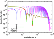
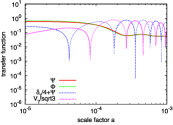
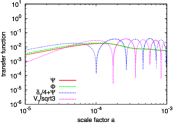
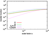
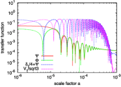
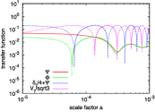
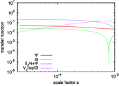
Figure 1: Perturbation evolution of the photon fluid and the metric. We showed the metric perturbations $\Psi$ (solid red) and $\Phi$ (dashed green), the photon effective temperature perturbation $\delta_{\gamma}/4+\Psi$ (dotted blue) and the photon velocity perturbation $V_{\gamma}/\sqrt{3}$(dot-dashed magenta). Positive and negative values are represented by thick and thin lines, respectively. From the top to bottom, each row corresponds to AD, CI and NID modes, in order. From the left to right, each column corresponds to three different scales $k=1$, $0.1$, $0.01$ Mpc^-1 in order.

Fig. 1 shows perturbation evolution of the photon fluid and the metric for the AD, CI and NID modes at three different scales ($k=1,~{}0.1$ and $0.01$ Mpc^-1), which are calculated by using a modified version of CAMB. In the figure, we plotted the metric perturbations $\Psi$ and $\Phi$, the photon effective temperature perturbation $\delta_{\gamma}/4+\Psi$ and the photon velocity perturbation $V_{\gamma}/\sqrt{3}$. As can be see from the figure, when perturbations enter the horizon, the photon fluids starts the acoustic oscillations, and at subhorizon scales the effective temperature $\delta_{\gamma}/4+\Psi$ keeps oscillating with an almost constant amplitude as long as it damps inside the diffusion scale. On the other hand, the photon velocity perturbation $V_{\gamma}/\sqrt{3}$ oscillates with the same amplitude but a phase shifted by $\pi/2$ compared with the effective temperature perturbation. We also note that gravitational potentials decay during the horizon crossing in RD.

Now we discuss the differences in the photon acoustic oscillation among the three different initial modes. The most distinct one that is found in Fig. 1 would be the difference in the oscillation phase for CI mode against other two modes. This originates from the fact that in CI mode oscillation starts with vanishing $\delta_{\gamma}$ at $\eta=0$, while oscillations of the other two modes start with non-vanishing $\delta_{\gamma}$. On the other hand, the differences between AD and NID modes may be less noticeable as their oscillation phases look similar. The most significant difference can be found in the change in the oscillation amplitudes between the horizon crossing. The amplitude of the acoustic oscillation gets boosted by the decay of gravitational potentials in the AD mode, which is less effective in the NID mode due to the initial smallness of the gravitational potentials.

In order to verify the above discussion, we adopt the semi-analytic solution of the acoustic oscillation derived in Ref. [47]. Under the adiabatic approximation, the WKB solution of Eq. (92) can be obtained as

$$\left[1+f(\eta)\right]^{1/4}\delta_{\gamma}(\eta) = \delta_{\gamma}(0)\cos kr_{s}(\eta)+\frac{\sqrt{3}}{k}\left[\dot{\delta}_{\gamma}(0)+\frac{1}{4}\dot{f}(0)\delta_{\gamma}(0)\right]\sin kr_{s}(\eta)$$ (94)

$$+\frac{4\sqrt{3}}{k}\int^{\eta}_{0}d\eta^{\prime}\left[1+f(\eta^{\prime})\right]^{3/4}\sin\left[kr_{s}(\eta)-kr_{s}(\eta^{\prime})\right]F(\eta^{\prime}),$$

where

$$r_{s}(\eta)=\int_{0}^{\eta}d\eta^{\prime}c_{s}(\eta^{\prime})$$ (95)

is the sound horizon of the photon-baryon fluid. In Eq. (94), the first and second terms correspond to the free damped oscillation which reflect the initial condition of photon density and velocity perturbations. On the other hand, the third term corresponds to the forced oscillation driven by the gravitational potentials. In the following discussion, the first, second, and third terms are called the cosine, sine and forced terms, respectively.

In Fig. 2, the time evolution of the photon density perturbation are plotted for the AD, CI and NID modes at $k=0.1\mathrm{Mpc}^{-1}$. In the figure, we have shown exact numerical solutions for $\delta_{\gamma}$ as well as the WKB solutions Eq. (94) obtained by adopting the numerically evaluated source term $F$. We can see that the WKB solution is in excellent agreement with the exact one, regardless of initial conditions. This allows us to understand correctly the physical origin that drives the evolution of photon perturbations by comparing the different terms in Eq. (94). For this purpose, we have also plotted the WKB cosine, sine and forced terms separately in the figure.

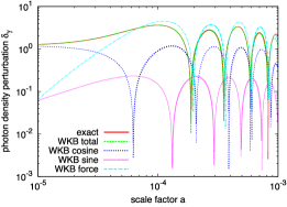
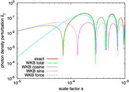
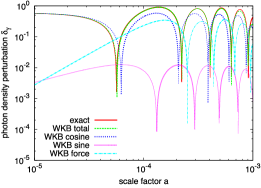
Figure 2: Time evolutions of the photon density perturbation $\delta_{\gamma}$ for AD (top), CI (middle) and NID (bottom) modes at $k=0.1~{}\mathrm{Mpc}^{-1}$. Plotted are the exact solution (solid red) the total WKB solution (dashed green), and three terms consisting the total WKB solution including the cosine term (dotted blue), sine term (dot-dahsed magenta) and term from the external force (dot-dot-dahsed light blue). Positive and negative values are represented by thick and thin lines, respectively.

For the AD mode, we see that the forced term dominates the acoustic oscillation and imprint of the initial cosine-like oscillation induced by $\delta_{\gamma}(0)$ is almost invisible. However, the external force also induces an acoustic oscillation with cosine-like phase, as the gravitational potentials also oscillate in a similar manner around the horizon crossing. Totally, the acoustic oscillation for AD mode can be regarded as a kind of forced oscillation with a cosine-type phase.

In the case of CI mode, the source term is also dominant as can be seen in Fig. 2. Since the gravitational potentials grow proportionally to $\eta$ at superhorizon scales as the density perturbations in CDM generates the curvature perturbation, they induce a sine-type acoustic oscillation rather than a cosine-type one. The acoustic oscillation in the CI mode can be regarded as a forced oscillation with a sine-type phase.

On the other hand, in the case of NID mode, the cosine term dominates the acoustic oscillation and the forced term is subdominant. This is in contrast to the previous two modes. This result comes from the fact that the gravitational potentials are initially small and grow little before the horizon crossing in NID mode. Therefore, the acoustic oscillation for the NID mode can be regarded as free oscillation with a cosine-type phase.

Smallness of the gravitational potentials also affect the perturbation evolution of photons after the recombination, when photons become collisionless and free-stream in the potentials which are dominantly formed by the CDM density perturbations. While gravitational potentials is constant deep in the matter dominated (MD) epoch, it is not fully MD just after the recombination, where the potentials decay during the horizon crossing. Effective temperature of free-streaming photons are boosted (or suppressed) due to the decay of the potentials $\Phi-\Psi$, which is well known as the early integrated Sachs-Wolfe (ISW) effect. In the AD and CI modes, the early ISW effect is significant, since their gravitational potentials are relatively large at the time of horizon crossing. Contrastively, the gravitational potentials are small in the NID mode, and hence their decay affects the photon perturbations little.

3.4 CMB temperature power spectrum

In Fig. 3, we plot the CMB temperature power spectrum ($C^{\mathrm{TT}}_{\ell}$) for the NID mode as well as those for other AD and CI modes for reference. The spectrum of the NID mode has distinct features coming from the fact that the evolution of photon perturbations in the NID mode is different from those in the AD and CI modes as we have seen above.

First of all, the positions of acoustic peaks in $C^{\mathrm{TT}}_{\ell}$ for the NID mode are more similar to those for the AD mode than those for the CI mode, which reflects the phase of acoustic oscillation in the each initial mode. In addition, the amplitude at the first acoustic peak ($\ell\simeq 300$) in the NID mode is almost same as that at the Sachs-Wolfe (SW) plateau ($\ell\lesssim 50$). This reflects the smallness of the gravitational potentials in the NID mode, where decay of the potentials does not boost the photon temperature significantly before and after the recombination. This should be contrasted to the AD mode, where the amplitude of $C^{\mathrm{TT}}_{\ell}$ at the acoustic regime is higher than that at the SW plateau.

Finally, we would like to give some brief comments on the effects of $\Delta N_{\mathrm{eff}}>0$ on the CMB power spectrum. At the sensitivity of current and near-future observations such as Planck, two characteristic changes from the case of $\Delta N_{\mathrm{eff}}=0$ would be important. One is that the RD epoch lasts longer and hence the expansion rate of the Universe becomes larger given at fixed redshifts. This enhances the early ISW effect and causes shifts in the acoustic peaks towards smaller angular scales. Another is that the free-streaming of neutrinos affects the perturbation evolution more significantly. This enhances the decay of the gravitational potentials before perturbations enter the sound horizon of the photon-baryon fluid and dampens the photon perturbations in the RD epoch. Thus, this effect suppresses the amplitude of $C^{\mathrm{TT}}_{\ell}$ at small angular scales. For more detailed discussion, we refer to e.g. Refs. [49, 9].

Figure 3: The CMB temperature power spectrum ($C^{\mathrm{TT}}_{\ell}$) for the AD, CI and NID modes.

4 Constraints from current observations

In this section we derive constraints on the isocurvature perturbations in the extra radiation using current cosmological observations. We adopt CMB data of WMAP 7-year result [50, 51, 52] and ACT [53, 54, 2] at small angular scales. While CMB power spectrum is the best probe for neutrino isocurvature perturbations, CMB itself contains considerable amount of parameter degeneracies among $S_{\mathrm{DR}}$, $N_{\mathrm{eff}}$ and other cosmological parameters. In order to solve the degeneracies, we also include data from the baryon acoustic oscillation (BAO) in the power spectrum of SDSS galaxies [55] and the direct measurement of the Hubble constant (H0) [56]. Hereafter, we will refer to sets of combined datasets of WMAP+ACT and WMAP+ACT+BAO+H0 as “CMB” and “ALL”, respectively.

The initial condition for structure formation in our model is a mixture of the AD and NID modes and these two initial modes can be in general correlated. Correlation functions of the initial modes, or equivalently the primordial perturbation spectra, form a symmetric matrix. We assume that the primordial perturbation spectra can be represented by power-law with same spectral indices. Then the primordial power spectra can be parametrized as follows, which is widely seen in literatures:

$$\begin{pmatrix}\mathcal{P}_{\zeta\zeta}(k)&\mathcal{P}_{\zeta S_{\mathrm{DR}}}(k)\\ \mathcal{P}_{S_{\mathrm{DR}}\zeta}(k)&\mathcal{P}_{S_{\mathrm{DR}}S_{\mathrm{DR}}}(k)\\ \end{pmatrix}=A_{s}\left(\frac{k}{k_{0}}\right)^{n_{s}-1}\begin{pmatrix}1-\alpha&\gamma\sqrt{\alpha(1-\alpha)}\\ \gamma\sqrt{\alpha(1-\alpha)}&\alpha\end{pmatrix},$$ (96)

where $\mathcal{P}_{AB}$ is the (cross-)power spectrum of initial perturbations $A$ and $B$ defined in Eq. (14), and $\gamma$ denotes the correlation parameter given in (13).

parameters	symbols	prior ranges
baryon density parameter	$\omega_{b}$	$0.005\to 0.1$
CDM density parameter	$\omega_{c}$	$0.01\to 0.99$
angular scale of sound horizon	$\theta_{s}$	$0.5\to 10$
optical depth of reionization	$\tau$	$0.01\to 0.8$
effective number of neutrino species	$N_{\mathrm{eff}}$	$(3.046\to 10)$
spectral index of primordial power spectra	$n_{s}$	$0.5\to 1.5$
amplitude of primordial power spectra	$\ln[10^{10}A_{s}]$	$2.7\to 4$
fraction of NID mode in primordial perturbations	$\alpha$	$0\to 1$
correlation between AD and NID modes	$\gamma$	$(-1\to 1)$
template amplitude of thermal SZ effect	$A_{SZ}$	$0\to 2$
template amplitude of Poisson distributed sources	$A_{p}$	$0\to 30$
template amplitude of clustered dust	$A_{cl}$	$0\to 15$

Table 2: Model parameters we constrain in our analysis. First nine from the top are the primary cosmological parameters, and rest three are the nuisance ones. The last column shows the range of top-hat priors for the parameters we adopt in the analysis. Note that the prior ranges of $N_{\mathrm{eff}}$ and $\gamma$, which are shown with parentheses, are only adopted when they are varied in the analysis (see text for more details).

In a most general case, the parameter space we explore consists of nine primary cosmological parameters $(\omega_{b},~{}\omega_{c},~{}\theta_{s},~{}\tau,~{}N_{\mathrm{eff}},~{}n_{s},~{}A_{s},~{}\alpha,~{}\gamma)$. Definitions of these parameters and top-hat priors we adopt in the parameter estimation are listed in Table 2. In particular, we take $N_{\mathrm{eff}}\geq 3.046$ since our model assumes that there are always the Standard Model neutrinos which are fully thermalized in the early Universe. In order to take account of foregrounds, we also include three nuisance parameters $A_{SZ}$, $A_{p}$, $A_{cl}$, which measure the amplitudes of power spectra from the Sunyaev-Zel’dovich (SZ) effect, point source, and clustered dust, respectively. We adopt the same template power spectra for these foregrounds as in the cosmological parameter estimation of Ref. [2]. In particular, templates for the SZ effect and clustered dust are based on Ref. [57].

There are several works where constraints on the NID mode are investigated [58, 59, 60, 62, 63]. $N_{\rm eff}$ is however fixed to the standard value $3.04$ in these analyses, so that our analysis explore a new parameter space which has not been investigated so far.

Parameter estimation is performed using a modified version of the publicly available CosmoMC code [64]. Convergence of a Markov chain Monte Carlo (MCMC) analysis is diagnosed by the Gelman-Rubin test $R-1<0.1$.

4.1 Fixed $\gamma$

parameters	CMB	ALL
$100\omega_{b}$	$2.35^{+0.10}_{-0.10}$	$2.25^{+0.05}_{-0.05}$
$\omega_{c}$	$0.135^{+0.016}_{-0.016}$	$0.133^{+0.012}_{-0.012}$
$\theta_{s}$	$1.038^{+0.003}_{-0.003}$	$1.037^{+0.003}_{-0.003}$
$\tau$	$0.089^{+0.007}_{-0.007}$	$0.085^{+0.007}_{-0.006}$
$N_{\mathrm{eff}}$ (95%CL)	$\leq 6.5$	$\leq 5.3$
$n_{s}$	$1.02^{+0.03}_{-0.03}$	$0.987^{+0.015}_{-0.015}$
$\ln[10^{10}A_{s}]$	$3.19^{+0.05}_{-0.05}$	$3.17^{+0.04}_{-0.04}$
$\alpha$ (95%CL)	$\leq 0.16$	$\leq 0.11$

Table 3: Constraints for the uncorrelated case ($\gamma=0$). We present mean values and 68 %CL intervals for cosmological parameters except for $N_{\mathrm{eff}}$ and $\alpha$, for which we present 95 %CL intervals since they are not bounded from below.

Figure 4: 68 % and 95 % CL constraints in $N_{\mathrm{eff}}$-$\alpha$ plane from the CMB (red solid) and ALL (green dashed) datasets. From top to bottom, shown are the constraints for the uncorrelated ($\gamma=0$), totally correlated ($\gamma=1$) and totally anti-correlated ($\gamma=-1$) cases. Note that the scales are not same among three panels.

Before varying all the nine primary parameters, we first fix $\gamma$ to $0$ or $\pm 1$ and vary other parameters. This allows us to investigate the constraints for the uncorrelated and totally (anti-)correlated cases separately.

Let us see from the constraints for the uncorrelated case ($\gamma=0$). Constraints on parameters are summarized in Table. 3. In particular, we obtain constraints $N_{\mathrm{eff}}\leq 5.3$ and $\alpha\leq 0.11$ at 95 %CL from the ALL dataset. We also show 2d constraints in $N_{\mathrm{eff}}$-$\alpha$ plane in Fig. 4. We see there is no strong degeneracy between $N_{\mathrm{eff}}$ and $\alpha$, so that constraints on these two parameters can be discussed separately. As is often discussed, current CMB observations essentially constrain the epoch of matter-radiation equality. Consequently, when $N_{\mathrm{eff}}$ is freely varied, $\omega_{c}$ and $N_{\mathrm{eff}}$ are strongly degenerated. This degeneracy is partially solved by including BAO and H0, which determine $\Omega_{m}$ and $H_{0}$ and hence lead to a better constraint on $N_{\mathrm{eff}}$. On the other hand, BAO and H0 data are also effective in the determination of $\omega_{b}$, which is strongly degenerated with $n_{s}$ because these two affect the relative height of the first and second peaks in a similar way. $\alpha$ is mostly degenerated with $\omega_{b}$ and $n_{s}$ because mixture of the NID mode $\alpha\neq 0$ affects the relative height of acoustic peaks with little effect on the peak positions. Thus, inclusion of BAO and H0 improves the constraint on $\alpha$ by solving its degeneracy with $\omega_{b}$ and $n_{s}$.

parameters	CMB	ALL
$100\omega_{b}$	$2.17^{+0.06}_{-0.06}$	$2.19^{+0.05}_{-0.05}$
$\omega_{c}$	$0.133^{+0.014}_{-0.014}$	$0.130^{+0.012}_{-0.012}$
$\theta_{s}$	$1.032^{+0.003}_{-0.003}$	$1.033^{+0.003}_{-0.003}$
$\tau$	$0.087^{+0.007}_{-0.007}$	$0.088^{+0.006}_{-0.007}$
$N_{\mathrm{eff}}$ (95%CL)	$\leq 5.4$	$\leq 5.1$
$n_{s}$	$0.97^{+0.02}_{-0.02}$	$0.972^{+0.015}_{-0.015}$
$\ln[10^{10}A_{s}]$	$3.16^{+0.04}_{-0.04}$	$3.15^{+0.04}_{-0.04}$
$\alpha$ (95%CL)	$\leq 0.012$	$\leq 0.011$

Table 4: Same table as in Table. 3 but for the totally correlated case ($\gamma=1$).

parameters	CMB	ALL
$100\omega_{b}$	$2.31^{+0.07}_{-0.07}$	$2.25^{+0.05}_{-0.04}$
$\omega_{c}$	$0.135^{+0.016}_{-0.016}$	$0.135^{+0.011}_{-0.011}$
$\theta_{s}$	$1.041^{+0.003}_{-0.003}$	$1.039^{+0.003}_{-0.003}$
$\tau$	$0.089^{+0.007}_{-0.007}$	$0.083^{+0.006}_{-0.006}$
$N_{\mathrm{eff}}$ (95%CL)	$\leq 6.2$	$\leq 5.2$
$n_{s}$	$1.01^{+0.02}_{-0.02}$	$0.987^{+0.013}_{-0.014}$
$\ln[10^{10}A_{s}]$	$3.10^{+0.04}_{-0.04}$	$3.11^{+0.04}_{-0.04}$
$\alpha$ (95%CL)	$\leq 0.013$	$\leq 0.007$

Table 5: Same table as in Table. 3 but for the anti-correlated case ($\gamma=-1$).

Let us then turn our attention to the totally correlated ($\gamma=1$) and anti-correlated ($\gamma=-1$) cases. Constraints on parameters for these two cases are summarized in Tables 4-5 and 2d constraints in $N_{\mathrm{eff}}$-$\alpha$ plane are also shown in Fig. 4. From the ALL dataset, we obtain $N_{\mathrm{eff}}\leq 5.4$ and $\alpha\leq 0.011$ for the totally correlated case and $N_{\mathrm{eff}}\leq 5.2$ and $\alpha\leq 0.007$ for the totally anti-correlated case, respectively. We first note that the constraints on $\alpha$ for the correlated cases are an order of magnitude tighter than those for the uncorrelated case. This is because given fixed $\alpha$, the NID mode affects the CMB power spectrum more significantly for the correlated cases than the uncorrelated one due to the power $P_{\zeta S_{\mathrm{DR}}}(k)$ arising from the cross correlation of the AD and NID modes. For small enough $\alpha$ of order e.g. $10^{-3}$, changes in the CMB power spectrum are somewhat similar in magnitude but opposite in the sign. However, data adopted in the analysis are not very constraining and relatively large $\alpha\simeq 0.01$ is allowed, where degeneracies of $\alpha$ with other parameters are different between the totally correlated and anti-correlated cases. For the totally correlated case ($\gamma=1$) $\alpha$ is not degenerated with other parameters strongly. This is the reason why the CMB constraint on $\alpha$ is little improved by including BAO and H0 for this case. On the other hand, $\alpha$ considerably is degenerated with $\omega_{c}$ and $n_{s}$ for the case of anti-correlated case ($\gamma=-1$). Better determination of $H_{0}$ and $\Omega_{m}$ due to inclusion of BAO and H0 directly tightens the constraint on $\omega_{c}$. Furthermore, $n_{s}$ itself is also strongly degenerated with $\omega_{c}$ and hence becomes more tightly constrained. Such the improvement in determination of $\omega_{c}$ and $n_{s}$ finally results in better constraints on $\alpha$.

4.2 Fixed $N_{\mathrm{eff}}$

As we have discussed in Introduction, there are several cosmological observations which independently show preference for a somewhat larger $N_{\mathrm{eff}}\simeq 4$ over the standard $N_{\mathrm{eff}}=3.04$ at around 2$\sigma$ level. When we look over the constraints obtained so far, it can be seen that such preference still survives, though with somewhat reduced significance, even if we include the possibility for the extra radiation to have isocurvature fluctuations which can be uncorrelated or totally (anti-)correlated with $\zeta$. This motivate us to investigate a generally correlated case with a fixed $N_{\mathrm{eff}}\neq 3.04$, for which we devote the rest of this section.

We perform MCMC analysis with $\gamma$ being varied and $N_{\mathrm{eff}}=4$ being fixed. We impose a top-hat prior on $\gamma$ with a range $[-1,1]$, and priors for other parameters are as listed in Table 2. This time we use only the ALL dataset and the resultant constraints are summarized in Table 6. In addition, the 2d constraint in the $\gamma$-$\alpha$ plane is shown in Fig. 5. As can be seen from the figure, we do not find any evidence for $\alpha>0$ and the extra radiation which is assumed to exist is consistent with purely AD perturbations. When $\gamma$ is marginalized, we obtain an upper bound $\alpha\leq 0.12$ at 95% CL, which is almost the same as one obtained for the uncorrelated case. We note that the constraint on $\gamma$ is of little importance, as long as $\alpha$ is consistent with zero.

parameters	ALL
$100\omega_{b}$	$2.24^{+0.05}_{-0.05}$
$\omega_{c}$	$0.129^{+0.004}_{-0.004}$
$\theta_{s}$	$1.037^{+0.003}_{-0.004}$
$\tau$	$0.086^{+0.007}_{-0.007}$
$n_{s}$	$0.983^{+0.013}_{-0.012}$
$\ln[10^{10}A_{s}]$	$3.16^{+0.06}_{-0.05}$
$\alpha$ (95%CL)	$\leq 0.12$
$\gamma$	$0.025^{+0.123}_{-0.080}$

Table 6: Constraints in the case that $N_{\rm eff}$ is set to $4$ and $\gamma$ is varied. We present mean values and 68 %CL intervals for cosmological parameters except for $\alpha$, for which we present 95 %CL intervals since it is not bounded from below.

Figure 5: 68 % and 95 % CL constraints in $\gamma$-$\alpha$ plane from ALL datasets.

4.3 Varying $N_{\mathrm{eff}}$ and $\gamma$

We finally present constraints for the most general case, where all nine primary parameters including $N_{\mathrm{eff}}$, $\alpha$ and $\gamma$ are varied simultaneously. Parameter constraints from ALL dataset are presented in Table 7. Compared with the case with fixed $N_{\mathrm{eff}}=4$ in Table 6, we can find that there is no significant degradation of constraints on parameters except for $\omega_{c}$, which is significantly degenerated with $N_{\mathrm{eff}}$. On the other hand, upper bound on $N_{\mathrm{eff}}$ is also as tight as those obtained for the case of fixed $\gamma$ in Section 4.1.

Marginalized constraints on $N_{\mathrm{eff}}$ and $\alpha$ are given as $N_{\mathrm{eff}}\leq 5.1$ and $\alpha\leq 0.11$ at 95 %CL. Following the results so far, we again do not find any signature for existence of non-vanishing isocurvature perturbations in extra radiations. 2d marginalized constraints for $N_{\mathrm{eff}}$, $\alpha$ and $\gamma$ are presented in Fig. 6.

parameters	ALL
$100\omega_{b}$	$2.24^{+0.05}_{-0.05}$
$\omega_{c}$	$0.131^{+0.011}_{-0.012}$
$\theta_{s}$	$1.037^{+0.003}_{-0.003}$
$\tau$	$0.083^{+0.006}_{-0.006}$
$N_{\mathrm{eff}}$ (95%CL)	$\leq 5.1$
$n_{s}$	$0.983^{+0.016}_{-0.015}$
$\ln[10^{10}A_{s}]$	$3.14^{+0.05}_{-0.05}$
$\alpha$ (95%CL)	$\leq 0.11$
$\gamma$	$0.07^{+0.11}_{-0.14}$

Table 7: Constraints for the generally correlated case ($-1\leq\gamma\leq 1$) from ALL dataset. We present mean values and 68 %CL intervals for cosmological parameters except for $N_{\mathrm{eff}}$ and $\alpha$, for which we present 95 %CL intervals since they are not bounded from below.

Figure 6: 68 % and 95 % CL constraints on $(N_{\mathrm{eff}},\alpha,\gamma)$ for generally correlated case from ALL dataset.

5 Implications

We have formulated a method for calculating the isocurvature perturbations in the extra radiation and derived observational constraints on them. Now let us apply the results to some concrete cases. Before discussing a concrete model, we derive formulae for some limiting cases for later convenience.

5.1 Limiting cases

5.1.1 Uncorrelated case

First, we suppose that the inflaton $\phi$ does not decay into $X$ ($r_{\phi}=1$) and the adiabatic perturbation is dominantly produced by the inflaton $(N_{\phi}\gg N_{\sigma})$. The $\sigma$ decays into $X$ with branching fraction of $1-r_{\sigma}$. Then one can easily imagine that the $X$ has an isocurvature perturbation that traces the primordial perturbation of $\sigma$.

In this case, from Eq. (58) we have

$$\Delta N_{\rm eff}\simeq\frac{3(1-r_{\sigma})R_{\sigma}}{c_{\nu}(1-(1-r_{\sigma})R_{\sigma})}\left(\frac{g_{*}(H=\Gamma_{\nu})}{g_{*}(H=\Gamma_{\sigma})}\right)^{1/3}.$$ (97)

and

$$\hat{S}_{\rm DR}\simeq\frac{(1-r_{\sigma})(1-R_{\sigma})(1-c_{\nu})}{\tilde{R}_{\rm DR}}\left(\frac{g_{*}(H=\Gamma_{\nu})}{g_{*}(H=\Gamma_{\sigma})}\right)^{1/3}\frac{2R\delta\sigma}{\sigma_{i}}.$$ (98)

with

$$\tilde{R}_{\rm DR}\simeq(1-r_{\sigma})R_{\sigma}\left(\frac{g_{*}(H=\Gamma_{\nu})}{g_{*}(H=\Gamma_{\sigma})}\right)^{1/3}+c_{\nu}(1-R_{\sigma}+r_{\sigma}R_{\sigma}).$$ (99)

In deriving (98), we have approximated parameters as $\hat{R}_{X}\simeq\tilde{R}_{X}\ll 1$ and $\hat{R}_{r}\simeq\tilde{R}_{r}$. Note that the condition $(N_{\phi}\gg N_{\sigma})$ leads to the constraint $2R\delta\sigma/\sigma_{i}\ll 10^{-4}$. In that limit the correlation parameter (61) is small : $|\gamma|\ll 1$. Thus the isocurvature perturbation is nearly uncorrelated with the curvature perturbation. It should be noticed that $S_{\rm DR}$ vanishes in the limit $R_{\sigma}\to 1$, since the inflaton contribution to the curvature perturbation becomes zero, as is clear from (28).

Fig. 7 shows constraints on $R_{\sigma}$-$r_{\sigma}$ plane for uncorrelated case. This is drawn by translating the results shown in the top panel of Fig. 4 into the constraint on $R_{\sigma}$ and $r_{\sigma}$, using (58) and (59). 1$\sigma$ and 2$\sigma$ allowed regions are shown by blue and orange, respectively. Contours of $\alpha$ and $\Delta N_{{\rm eff}}$ are also shown. In this figure $2R\delta\sigma/\sigma_{i}=0.1\times\zeta_{\phi}\simeq 5\times 10^{-6}$ and $g_{*}(H=\Gamma_{\sigma})=100$ are fixed.

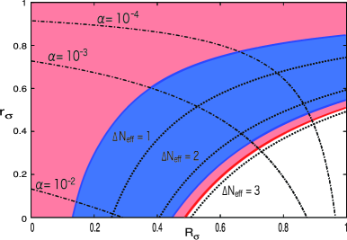
Figure 7: Constraints on $R_{\sigma}$-$r_{\sigma}$ plane for uncorrelated case. 1$\sigma$ and 2$\sigma$ allowed regions are shown by blue and orange, respectively. Contours of $\alpha$ and $\Delta N_{{\rm eff}}$ are also shown. In this figure $2R\delta\sigma/\sigma_{i}\simeq 5\times 10^{-6}$ is fixed.

5.1.2 Totally anti-correlated case

Next, suppose that the $\sigma$ does not decay into $X$, i.e., $r_{\sigma}=1$, and $\sigma$ dominantly produces the curvature perturbation ($N_{\phi}\ll N_{\sigma}$) : $\sigma$ truly takes a role of curvaton. The inflaton $\phi$ is assumed to decay into $X$ with branching fraction of $1-r_{\phi}$. Then the extra radiation $X$ produced by the inflaton decay is expected to have isocurvature perturbation correlated with the curvature one.

In this case we have

$$\Delta N_{\rm eff}\simeq\frac{3(1-r_{\phi})(1-R_{\sigma})}{c_{\nu}(r_{\phi}(1-R_{\sigma})+R_{\sigma})}\left(\frac{g_{*}(H=\Gamma_{\nu})}{g_{*}(H=\Gamma_{\sigma})}\right)^{1/3},$$ (100)

and

$$\hat{S}_{\rm DR}=-\frac{(1-r_{\phi})(1-R_{\sigma})(1-c_{\nu})}{\tilde{R}_{\rm DR}}\left(\frac{g_{*}(H=\Gamma_{\nu})}{g_{*}(H=\Gamma_{\sigma})}\right)^{1/3}\frac{2R\delta\sigma}{\sigma_{i}}.$$ (101)

with

$$\tilde{R}_{\rm DR}\simeq(1-r_{\phi})(1-R_{\sigma})\left(\frac{g_{*}(H=\Gamma_{\nu})}{g_{*}(H=\Gamma_{\sigma})}\right)^{1/3}+c_{\nu}(r_{\phi}+R_{\sigma}-r_{\phi}R_{\sigma}).$$ (102)

In deriving (101), we have approximated parameters as $\hat{R}_{X}\simeq\tilde{R}_{X}\ll 1$ and $\hat{R}_{r}\simeq\tilde{R}_{r}$. Notice that we have the condition $2R\delta\sigma/\sigma_{i}\simeq 1.5\times 10^{-4}$ in order for the curvaton to produce the curvature perturbation. In this limit, the correlation parameter (61) becomes $\gamma\simeq-1$ : the isocurvature perturbation is almost totally anti-correlated with the curvature perturbation. Also we need $R\gtrsim 0.01$ in order not to have too large non-Gaussianity.

Fig. 8 shows constraints on $R_{\sigma}$-$r_{\phi}$ plane for totally anti-correlated case. This figure is obtained by converting bottom panel of Fig. 4 using (58) and (59). 2$\sigma$ allowed regions are shown by orange. Any values of $R_{\sigma}$ and $r_{\phi}$ are excluded at 1$\sigma$ level. In this figure, contours of both $\alpha$ and $\Delta N_{{\rm eff}}$ are shown. Note that in the case of $r_{\sigma}=1$, the following relation between $\alpha$ and $\Delta N_{\rm eff}$ is satisfied.

$$\sqrt{\frac{\alpha}{1-\alpha}}=-\frac{\hat{S}_{\rm DR}}{\hat{\zeta}}=3(1-\hat{c}_{\nu})\frac{\Delta N_{\rm eff}}{3+\Delta N_{\rm eff}},$$ (103)

which is derived from (58), (59) and (60). Here $g_{*}(H=\Gamma_{\sigma})$ is set to $100$ in this figure.

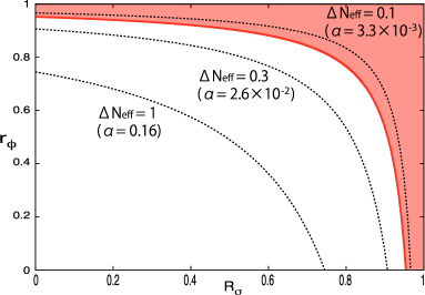
Figure 8: Constraints on $R_{\sigma}$-$r_{\phi}$ plane for totally anti-correlated case. 2$\sigma$ allowed regions are shown by orange. There is no 1$\sigma$ allowed region.

5.2 Particle physics model

A model to explain $\Delta N_{\rm eff}\simeq 1$ was proposed in Ref. [17]. It is based on the supersymmetric (SUSY) extension of the axion model. The axion is a pseudo Nambu-Goldstone boson associated with the spontaneous breakdown of the Peccei-Quinn (PQ) symmetry, which is introduced in order to solve the strong CP problem in quantum chromo dynamics [65]. In a SUSY axion model, there exists a scalar field $\sigma$, called saxion, which is a scalar partner of the PQ axion [66]. The saxion can naturally have a mass of the order of the gravitino, which is the superpartner of the graviton, and it can be $\mathcal{O}$(keV)-$\mathcal{O}$(TeV). The saxion can have a large initial amplitude $\sigma_{i}$ during inflation, and may obtain quantum fluctuations of $\delta\sigma\sim H_{\rm inf}/(2\pi)$ since its mass is much smaller than the Hubble scale during inflation. Therefore, the saxion is a candidate for the curvaton. The saxion decay mode depends on the model (see e.g. Refs. [67, 68, 69, 70, 71, 72]). We consider following two cases : the saxion dominantly decays into two axions $(\sigma\to aa)$ and into the Higgs boson pair $(\sigma\to hh)$. The former situation is typically realized in the KSVZ axion model [73] and leads to the uncorrelated isocurvature perturbation in the relativistic axion particles if the curvature perturbation is dominantly sourced by the inflaton. The latter possibility appears in the DFSZ axion model [74]. In this case, the saxion can take a role of the curvaton and thermally produced axions after the inflaton decay have correlated isocurvature perturbations. In the axion model, the axion also has an isocurvature perturbation which results in the CDM isocurvature mode. We do not discuss it in detail since it can be reduced by tuning the initial misalignment angle.

5.2.1 SUSY KSVZ axion model

First, let us consider the case where the saxion decays into two axions. This is often the case in the KSVZ axion model [73]. The decay rate of this process is given by

$$\Gamma(\sigma\to 2a)=\frac{f^{2}}{64\pi}\frac{m_{\sigma}^{3}}{f_{a}^{2}},$$ (104)

where $f_{a}$ denotes the PQ symmetry breaking scale, which is constrained as $10^{9}$GeV $\lesssim f_{a}\lesssim 10^{12}$GeV and $f$ is a typically $\mathcal{O}(1)$ constant. Hereafter we take $f=1$. The temperature at the saxion decay is calculated as

$$T_{\sigma}\simeq 100~{}{\rm MeV}\left(\frac{100}{g_{*}(T_{\sigma})}\right)^{1/4}\left(\frac{m_{\sigma}}{100{\rm GeV}}\right)^{3/2}\left(\frac{10^{12}{\rm GeV}}{f_{a}}\right).$$ (105)

The saxion also decays into gluons if kinematically allowed. The branching ratio of the saxion into gluons, $r_{\sigma}$, is given by

$$r_{\sigma}\simeq\frac{2\alpha_{s}^{2}}{\pi^{2}}\sim 3\times 10^{-3},$$ (106)

and hence very small. Nonthermal axions produced by the saxion decay is regarded as an extra radiation $X$, since the PQ axion has only extremely weak interaction with ordinary matter and its mass is very small. The abundance of the saxion coherent oscillation is given by

$$\begin{split}\frac{\rho_{\sigma}}{s}=\frac{1}{8}T_{\rm R}\left(\frac{\sigma_{i}}{M_{\rm P}}\right)^{2}\simeq 2\times 10^{-8}{\rm GeV}\left(\frac{T_{\rm R}}{10^{6}{\rm GeV}}\right)\left(\frac{\sigma_{i}}{10^{12}{\rm GeV}}\right)^{2},\end{split}$$ (107)

for $m_{\sigma}>\Gamma_{\phi}$ and

$$\begin{split}\frac{\rho_{\sigma}}{s}=\frac{1}{8}T_{\rm osc}\left(\frac{\sigma_{i}}{M_{\rm P}}\right)^{2}\simeq 2\times 10^{-6}{\rm GeV}\left(\frac{m_{\sigma}}{100{\rm GeV}}\right)^{1/2}\left(\frac{\sigma_{i}}{10^{12}{\rm GeV}}\right)^{2},\end{split}$$ (108)

for $m_{\sigma}<\Gamma_{\phi}$ where $s$ denotes the entropy density, $T_{\rm R}$ the reheating temperature after inflation which is related to the inflaton decay rate $\Gamma_{\phi}$ as $T_{\rm R}=(10/\pi^{2}g_{*})^{1/4}\sqrt{\Gamma_{\phi}M_{P}}$ and $T_{\rm osc}\equiv(10/\pi^{2}g_{*})^{1/4}\sqrt{m_{\sigma}M_{P}}$. Thus $R\simeq(3/4)R_{\sigma}=3\rho_{\sigma}/(4\rho_{\rm tot})$ at the $\sigma$ decay is estimated as

$$\begin{split}R=\frac{1}{8}\frac{T_{\rm R}}{T_{\sigma}}\frac{\sigma_{i}^{2}}{M_{\rm P}^{2}}\simeq 2\times 10^{-4}\left(\frac{T_{\rm R}}{10^{6}{\rm GeV}}\right)\left(\frac{1{\rm GeV}}{m_{\sigma}}\right)^{3/2}\left(\frac{f_{a}}{10^{12}{\rm GeV}}\right)^{3}\left(\frac{\sigma_{i}}{f_{a}}\right)^{2},\end{split}$$ (109)

for $R\ll 1$ and $m_{\sigma}>\Gamma_{\phi}$ and

$$\begin{split}R=\frac{1}{8}\frac{T_{\rm osc}}{T_{\sigma}}\frac{\sigma_{i}^{2}}{M_{\rm P}^{2}}\simeq 2\times 10^{-3}\left(\frac{1{\rm GeV}}{m_{\sigma}}\right)\left(\frac{f_{a}}{10^{12}{\rm GeV}}\right)^{3}\left(\frac{\sigma_{i}}{f_{a}}\right)^{2},\end{split}$$ (110)

for $R\ll 1$ and $m_{\sigma}<\Gamma_{\phi}$. Assuming that the inflaton decays only to the visible sector $(r_{\phi}=1)$, $\Delta N_{\rm eff}$ and $S_{\rm DR}$ are obtained by substituting (109) into Eqs. (97) and (98). The $\Delta N_{\rm eff}$ is estimated as

$$\Delta N_{\rm eff}\simeq\frac{43}{7}\frac{R_{\sigma}}{1-R_{\sigma}}\left(\frac{g_{*}(H=\Gamma_{\nu})}{g_{*}(H=\Gamma_{\sigma})}\right)^{1/3}.$$ (111)

Therefore, both $\Delta N_{\rm eff}$ and $\hat{S}_{\rm DR}$ can have sizable values depending on model parameters.

5.2.2 SUSY DFSZ axion model

Next let us consider the case where the saxion dominantly decays into a Higgs boson pair, as is realized in the DFSZ axion model [74]. In this case, the saxion can take a role of the curvaton. The decay rate of this process is given by

$$\Gamma(\sigma\to 2h)=\frac{1}{8\pi}\frac{m_{\sigma}^{3}}{f_{a}^{2}}\left(\frac{\mu}{m_{\sigma}}\right)^{4},$$ (112)

where $\mu$ denotes the so-called $\mu$-parameter in SUSY, which gives the higgsino mass. If this is the dominant mode, the invisible branching ratio into an axion pair is estimated as

$$1-r_{\sigma}=\frac{1}{8}\left(\frac{m_{\sigma}}{\mu}\right)^{4},$$ (113)

which can be very small if $\mu>m_{\sigma}$, and we have $r_{\sigma}\simeq 1$. However, even if we neglect the nonthermal axions produced by the saxion decay, there is another contribution from thermal production during reheating. For simplicity we consider the case that axions are thermalized after the inflaton decays, which occurs if the reheating temperature satisfies [75]

$$T_{\rm R}\gtrsim T_{\rm D}\equiv 9.6\times 10^{6}~{}{\rm GeV}\left(\frac{f_{a}}{10^{10}{\rm GeV}}\right)^{2.246}.$$ (114)

If the reheating temperature is higher than this, axions are thermalized for $T>T_{\rm D}$ and decouple from thermal bath at $T\simeq T_{\rm D}$. At this moment, the fraction of the axion energy density relative to the total radiation energy density is given by $g_{*}(T=T_{\rm D})^{-1}$. Thus we can effectively regard that the inflaton decayed into axions with branching fraction of $\simeq g_{*}(T=T_{\rm D})^{-1}$. Therefore, we can replace $1-r_{\phi}$, which is defined at the curvaton (saxion) decay, with

$$1-r_{\phi}=\frac{1}{g_{*}(T=T_{\rm D})}\left(\frac{g_{*}(H=\Gamma_{\sigma})}{g_{*}(T=T_{\rm D})}\right)^{1/3}.$$ (115)

From Eq. (100), we obtain a well known expression for the $\Delta N_{\rm eff}$ for thermalized species (see e.g., Ref. [19])

$$\Delta N_{\rm eff}\simeq\frac{3(1-r_{\phi})}{c_{\nu}}\left(\frac{g_{*}(H=\Gamma_{\nu})}{g_{*}(H=\Gamma_{\sigma})}\right)^{1/3}=\frac{4}{7}\left(\frac{g_{*}(H=\Gamma_{\nu})}{g_{*}(T=T_{\rm D})}\right)^{4/3},$$ (116)

for $R_{\sigma}\ll 1$. Otherwise, the saxion decay dilutes the thermally produced axions to a negligible level. Those thermal axions have an anti-correlated isocurvature perturbation to the curvature perturbation, since the latter is assumed to be produced dominantly by the curvaton. The magnitude of the isocurvature perturbation in this case is given by (101).

6 Conclusions and discussion

In this paper, we have investigated isocurvature perturbations in an extra radiation component. We have firstly formulated how primordial isocurvature perturbations between the extra radiation and the Standard Model radiation can be generated from fluctuations of two scalar fields in the inflationary Universe. We gave a detailed description of what isocurvature perturbations in the dark radiation are generated. Our derivation of the isocuravature perturbations is based on the $\delta N$ formalism and fully non-linear. We have also pointed out that non-Gaussianities can be generated in such isocurvature perturbations, which are to be investigated in more detail in future works. It would be straightforward to extend our formulation for cases with three or more fields. We have also discussed observational signatures of the isocurvature perturbations in the extra radiation. We have pointed out that our model leads to distinct features in the CMB power spectrum which are different from those predicted by the ordinary curvature and CDM/baryon isocurvature perturbations. We have shown that that our model can be constrained from current cosmological observations. Roughly speaking, CMB combined with BAO and the direct measurement of $H_{0}$ gives constraints on the abundance of the extra radiation and the amplitude of its isocurvature perturbations as $3\leq N_{\mathrm{eff}}\leq 5$ and $\alpha\leq 0.1~{}(0.01)$ for the uncorrelated (totally correlated/anti-correlated) case. These are also translated into constraints on some limiting scenarios which can be realized in models based on particle physics such as SUSY axion model.

Our model will be tested more precisely by cosmological observations which are ongoing or projected in the near future. In particular, CMB power spectrum from the Planck survey is expected to improve constraints on both $N_{\mathrm{eff}}$ and $\alpha$ by an order of magnitude. Furthermore, non-Gaussianities and other observational signatures would be also informative.

Appendix A Extra radiation production after BBN

So far we have assumed that the $\sigma$ decays before the BBN and hence the neutrino freezeout epoch. This may not necessarily be the case. If the $\sigma$ mainly decays into the $X$ particle without producing a significant amount of visible particles, the decay of $\sigma$ does not upset BBN. Thus it may be possible that the $\sigma$ decays after the neutrino freezeout but well before the recombination. In this case the produced $X$ particles contribute to $\Delta N_{\rm eff}$ measured from CMB but does not affect $\Delta N_{\rm eff}$ measured from BBN. Examples of concrete models were proposed in Ref. [17, 20]. In this appendix we derive a formula in such a case.

The scenario we are considering here is summarized in Table 8. The curvaton $\sigma$ decays after BBN begins. if the decay is too late, the effects of extra radiation on the CMB and LSS are much more different and we do not consider such a case. Thus we restrict the lifetime of the curvaton to be less than $\sim 10^{8}~{}{\rm sec}$. By taking the uniform density slice at the curvaton decay, we have following relations

$$\rho_{X}^{(\phi)}(\vec{x})+(1-r_{\sigma}^{(\gamma)}-r_{\sigma}^{(\nu)})\rho_{\sigma}(\vec{x})=\rho_{X}(\vec{x}),$$ (117)

$$\rho_{\gamma}^{(\phi)}(\vec{x})+r_{\sigma}^{(\gamma)}\rho_{\sigma}(\vec{x})=\rho_{\gamma}(\vec{x}),$$ (118)

$$\rho_{\nu}^{(\phi)}(\vec{x})+r_{\sigma}^{(\nu)}\rho_{\sigma}(\vec{x})=\rho_{\nu}(\vec{x}),$$ (119)

$$\rho_{\gamma}^{(\phi)}(\vec{x})+\rho_{\nu}^{(\phi)}(\vec{x})+\rho_{X}^{(\phi)}(\vec{x})+\rho_{\sigma}(\vec{x})=\rho_{\rm tot}(\vec{x})(=\bar{\rho}_{\rm tot}).$$ (120)

Here $r_{\sigma}^{(\gamma)}$ and $r_{\sigma}^{(\nu)}$ are the branching ratios of $\sigma$ into the photon and neutrino. The curvature perturbation of each component is related to its background value as

$$\rho_{X}^{(\phi)}(\vec{x})=\bar{\rho}_{X}^{(\phi)}e^{4(\zeta_{\phi}-\hat{\zeta})},$$ (121)

$$\rho_{\gamma}^{(\phi)}(\vec{x})=\bar{\rho}_{\gamma}^{(\phi)}e^{4(\zeta_{\phi}-\hat{\zeta})},$$ (122)

$$\rho_{\nu}^{(\phi)}(\vec{x})=\bar{\rho}_{\nu}^{(\phi)}e^{4(\zeta_{\phi}-\hat{\zeta})},$$ (123)

$$\rho_{\sigma}(\vec{x})=\bar{\rho}_{\sigma}e^{3(\zeta_{\sigma}-\hat{\zeta})}.$$ (124)

The requirement that the curvaton decay should not spoil BBN sets strong constraint on the branching ratio into the photon [76] and neutrino [77]. Therefore we can safely set $r_{\sigma}^{(\gamma)}=r_{\sigma}^{(\nu)}=0$ since we are considering the case where the curvaton energy density is not negligible at the curvaton decay. Then we soon find

$$\zeta_{\gamma}=\zeta_{\phi},~{}~{}~{}\zeta_{\nu}=\zeta_{\phi}.$$ (125)

The total curvature perturbation and the curvature perturbation in $X$ are found to be

$$\begin{split}\hat{\zeta}&=\zeta_{\phi}+R(\zeta_{\sigma}-\zeta_{\phi})+\frac{1}{2}R(1-R)(3+R)(\zeta_{\phi}-\zeta_{\sigma})^{2},\\ \zeta_{X}&=\frac{1}{4R_{X}}\left[(4R_{X}^{(\phi)}+(1-R)R_{X}^{(\sigma)})\zeta_{\phi}+(3+R)R_{X}^{(\sigma)}\zeta_{\sigma}\right]\\ &~{}~{}+\frac{(3+R)R_{X}^{(\sigma)}}{8R_{X}^{2}}\left[(1+R)(3-R)R_{X}^{(\phi)}+(1-R)RR_{X}^{(\sigma)}\right](\zeta_{\phi}-\zeta_{\sigma})^{2},\end{split}$$ (126)

where $R$ is defined by Eq. (29) with $R_{\sigma}\equiv\bar{\rho}_{\sigma}/\bar{\rho}_{\rm tot}|_{H=\Gamma_{\sigma}}$. Notice also that $R_{X}^{(\sigma)}=R_{\sigma}$ and $R_{r}^{(\sigma)}=0$ in the present case. Other quantities are also defined as Eq. (27). Since there are no changes in the relativistic degrees of freedom after the curvaton decay, the expression (126) gives the final curvature perturbation. The DR energy density is defined by

$$\rho_{\nu}^{(\phi)}(\vec{x})+\rho_{X}^{(\phi)}(\vec{x})+\rho_{\sigma}(\vec{x})=\rho_{\rm DR}(\vec{x}),$$ (127)

on the uniform density slice, where $\rho_{\rm DR}(\vec{x})=\bar{\rho}_{\rm DR}e^{4(\zeta_{\rm DR}-\hat{\zeta})}$. The DR isocurvature perturbation is calculated as

$$\begin{split}\hat{S}_{\rm DR}&\equiv 3(\zeta_{\rm DR}-\hat{\zeta})\\ &=-3\frac{R_{r}R}{R_{\rm DR}}(1-\hat{c}_{\nu})\left[-(\zeta_{\sigma}-\zeta_{\phi})+\left\{\frac{(R-3)(R+1)}{2}+\frac{2R}{R_{\rm DR}}(1+R_{\rm DR})\right\}(\zeta_{\sigma}-\zeta_{\phi})^{2}\right],\end{split}$$ (128)

where $\hat{c}_{\nu}$ is given in Eq. (51), $R_{r}=(\bar{\rho}_{\gamma}+\bar{\rho}_{\nu})/\bar{\rho}_{\rm tot}$ and $R_{\rm DR}=(\bar{\rho}_{X}+\bar{\rho}_{\nu})/\bar{\rho}_{\rm tot}$ evaluated after the curvaton decay.

epoch	component	energy transfer
$\Gamma_{\phi}<H$	$\phi$, $\sigma$	$\phi\to X^{(\phi)}+r^{(\phi)}$
$\Gamma_{\nu}<H<\Gamma_{\phi}$	$X^{(\phi)}$, $r^{(\phi)}$, $\sigma$	$r^{(\phi)}\to\nu+r_{e}$
$\Gamma_{e^{\pm}}<H<\Gamma_{\nu}$	$X^{(\phi)}$, $\nu$, $r_{e}$, $\sigma$	$e^{\pm}\to\gamma$
$\Gamma_{\sigma}<H<\Gamma_{e^{\pm}}$	$X^{(\phi)}$, $\nu$, $\gamma$, $\sigma$	$\sigma\to X^{(\sigma)}$
$H<\Gamma_{\sigma}$	$X$, $\nu$, $\gamma$ (${\rm DR}=X+\nu$)

Table 8: Same as Table 1 but for the case of $\Gamma_{\sigma}<\Gamma_{e^{\pm}}$. The $\sigma$ is assumed to dominantly decay into $X$.

The extra effective number of neutrino species, $\Delta N_{\rm eff}$, is given by

$$\Delta N_{\rm eff}=3\frac{\rho_{X}}{\rho_{\nu}}=\frac{3R_{\sigma}}{\hat{c}_{\nu}R_{r}}.$$ (129)

This is explicitly evaluated as

$$\Delta N_{\rm eff}\simeq 1.1\left(\frac{1{\rm keV}}{T_{\sigma}}\right)\left(\frac{\rho_{\sigma}/s}{10^{-7}{\rm GeV}}\right).$$ (130)

References

- [1] E. Komatsu et al. [ WMAP Collaboration ], Astrophys. J. Suppl. 192, 18 (2011). [arXiv:1001.4538 [astro-ph.CO]].
- [2] J. Dunkley, R. Hlozek, J. Sievers et al., [arXiv:1009.0866 [astro-ph.CO]].
- [3] R. Keisler, C. L. Reichardt, K. A. Aird, B. A. Benson, L. E. Bleem, J. E. Carlstrom, C. L. Chang, H. M. Cho et al., [arXiv:1105.3182 [astro-ph.CO]].
- [4] A. X. Gonzalez-Morales, R. Poltis, B. D. Sherwin and L. Verde, arXiv:1106.5052 [astro-ph.CO].
- [5] J. Hamann, arXiv:1110.4271 [astro-ph.CO].
- [6] G. Mangano, A. Melchiorri, O. Mena, G. Miele, A. Slosar, JCAP 0703, 006 (2007). [astro-ph/0612150].
- [7] M. Cirelli, A. Strumia, JCAP 0612, 013 (2006). [astro-ph/0607086].
- [8] V. Simha, G. Steigman, JCAP 0806, 016 (2008). [arXiv:0803.3465 [astro-ph]].
- [9] K. Ichikawa, T. Sekiguchi, T. Takahashi, Phys. Rev. D78, 083526 (2008). [arXiv:0803.0889 [astro-ph]].
- [10] Y. I. Izotov, T. X. Thuan, Astrophys. J. 710, L67-L71 (2010). [arXiv:1001.4440 [astro-ph.CO]].
- [11] E. Aver, K. A. Olive, E. D. Skillman, JCAP 1005, 003 (2010). [arXiv:1001.5218 [astro-ph.CO]]; E. Aver, K. A. Olive, E. D. Skillman, [arXiv:1012.2385 [astro-ph.CO]].
- [12] J. Hamann, S. Hannestad, G. G. Raffelt, I. Tamborra, Y. Y. Y. Wong, Phys. Rev. Lett. 105, 181301 (2010). [arXiv:1006.5276 [hep-ph]].
- [13] S. H. Hansen, G. Mangano, A. Melchiorri, G. Miele, O. Pisanti, Phys. Rev. D65, 023511 (2002). [astro-ph/0105385].
- [14] M. Kawasaki, F. Takahashi, M. Yamaguchi, Phys. Rev. D66, 043516 (2002). [hep-ph/0205101].
- [15] L. A. Popa, A. Vasile, JCAP 0806, 028 (2008). [arXiv:0804.2971 [astro-ph]].
- [16] G. Mangano, G. Miele, S. Pastor, O. Pisanti, S. Sarikas, JCAP 1103, 035 (2011). [arXiv:1011.0916 [astro-ph.CO]].
- [17] K. Ichikawa, M. Kawasaki, K. Nakayama, M. Senami, F. Takahashi, JCAP 0705, 008 (2007). [hep-ph/0703034 [HEP-PH]].
- [18] L. M. Krauss, C. Lunardini, C. Smith, [arXiv:1009.4666 [hep-ph]].
- [19] K. Nakayama, F. Takahashi, T. T. Yanagida, Phys. Lett. B697, 275-279 (2011). [arXiv:1010.5693 [hep-ph]].
- [20] W. Fischler, J. Meyers, Phys. Rev. D83, 063520 (2011). [arXiv:1011.3501 [astro-ph.CO]].
- [21] P. C. de Holanda, A. Y. .Smirnov, [arXiv:1012.5627 [hep-ph]].
- [22] D. H. Lyth, D. Wands, Phys. Lett. B524, 5-14 (2002). [hep-ph/0110002]; T. Moroi, T. Takahashi, Phys. Lett. B522, 215-221 (2001). [hep-ph/0110096]; K. Enqvist, M. S. Sloth, Nucl. Phys. B626, 395-409 (2002). [hep-ph/0109214].
- [23] M. Kawasaki, K. Nakayama, T. Sekiguchi, T. Suyama, F. Takahashi, JCAP 0811, 019 (2008). [arXiv:0808.0009 [astro-ph]].
- [24] M. Kawasaki, K. Nakayama, F. Takahashi, JCAP 0901, 002 (2009). [arXiv:0809.2242 [hep-ph]].
- [25] D. Langlois, F. Vernizzi, D. Wands, JCAP 0812, 004 (2008). [arXiv:0809.4646 [astro-ph]].
- [26] M. Kawasaki, K. Nakayama, T. Sekiguchi, T. Suyama, F. Takahashi, JCAP 0901, 042 (2009). [arXiv:0810.0208 [astro-ph]].
- [27] C. Hikage, K. Koyama, T. Matsubara, T. Takahashi, M. Yamaguchi, Mon. Not. Roy. Astron. Soc. 398, 2188-2198 (2009). [arXiv:0812.3500 [astro-ph]].
- [28] E. Kawakami, M. Kawasaki, K. Nakayama, F. Takahashi, JCAP 0909, 002 (2009). [arXiv:0905.1552 [astro-ph.CO]].
- [29] C. Hikage, D. Munshi, A. Heavens, P. Coles, Mon. Not. Roy. Astron. Soc. 404, 1505-1511 (2010). [arXiv:0907.0261 [astro-ph.CO]].
- [30] K. Nakayama, F. Takahashi, Phys. Lett. B679, 436-439 (2009). [arXiv:0907.0834 [hep-ph]].
- [31] D. Langlois, A. Lepidi, JCAP 1101, 008 (2011). [arXiv:1007.5498 [astro-ph.CO]].
- [32] D. Langlois, T. Takahashi, JCAP 1102, 020 (2011). [arXiv:1012.4885 [astro-ph.CO]].
- [33] D. Langlois, B. van Tent, [arXiv:1104.2567 [astro-ph.CO]].
- [34] W. Hu, Phys. Rev. D 59, 021301 (1999) [arXiv:astro-ph/9809142].
- [35] M. Sasaki, E. D. Stewart, Prog. Theor. Phys. 95, 71-78 (1996). [astro-ph/9507001].
- [36] D. H. Lyth, K. A. Malik, M. Sasaki, JCAP 0505, 004 (2005). [astro-ph/0411220].
- [37] D. Wands, K. A. Malik, D. H. Lyth, A. R. Liddle, Phys. Rev. D62, 043527 (2000). [astro-ph/0003278].
- [38] M. Sasaki, J. Valiviita, D. Wands, Phys. Rev. D74, 103003 (2006). [astro-ph/0607627].
- [39] K. Enqvist, S. Nurmi, JCAP 0510, 013 (2005). [astro-ph/0508573]; K. Enqvist, T. Takahashi, JCAP 0809, 012 (2008). [arXiv:0807.3069 [astro-ph]]; Q. -G. Huang, Y. Wang, JCAP 0809, 025 (2008). [arXiv:0808.1168 [hep-th]].
- [40] M. Kawasaki, K. Nakayama, F. Takahashi, JCAP 0901, 026 (2009). [arXiv:0810.1585 [hep-ph]]; P. Chingangbam, Q. -G. Huang, JCAP 0904, 031 (2009). [arXiv:0902.2619 [astro-ph.CO]]; Q. -G. Huang, JCAP 1011, 026 (2010). [arXiv:1008.2641 [astro-ph.CO]].
- [41] K. Ichikawa, T. Suyama, T. Takahashi, M. Yamaguchi, Phys. Rev. D78, 023513 (2008). [arXiv:0802.4138 [astro-ph]].
- [42] M. Bucher, K. Moodley, N. Turok, Phys. Rev. D62, 083508 (2000). [astro-ph/9904231].
- [43] R. Trotta, [astro-ph/0410115].
- [44] A. Lewis, A. Challinor, A. Lasenby, Astrophys. J. 538, 473-476 (2000). [astro-ph/9911177].
- [45] C. Gordon, A. Lewis, Phys. Rev. D67, 123513 (2003). [astro-ph/0212248].
- [46] M. Kawasaki, T. Sekiguchi, T. Takahashi, [arXiv:1104.5591 [astro-ph.CO]].
- [47] W. Hu, N. Sugiyama, Astrophys. J. 444, 489-506 (1995). [astro-ph/9407093].
- [48] C. Zunckel, P. Okouma, S. M. Kasanda, K. Moodley and B. A. Bassett, Phys. Lett. B 696, 433 (2011) [arXiv:1006.4687 [astro-ph.CO]].
- [49] S. Bashinsky, U. Seljak, Phys. Rev. D69, 083002 (2004). [astro-ph/0310198].
- [50] B. Gold et al., Astrophys. J. Suppl. 192, 15 (2011) [arXiv:1001.4555 [astro-ph.GA]].
- [51] D. Larson et al., Astrophys. J. Suppl. 192, 16 (2011) [arXiv:1001.4635 [astro-ph.CO]].
- [52] N. Jarosik et al., Astrophys. J. Suppl. 192, 14 (2011) [arXiv:1001.4744 [astro-ph.CO]].
- [53] A. Hajian et al., arXiv:1009.0777 [astro-ph.CO].
- [54] S. Das et al., Astrophys. J. 729, 62 (2011) [arXiv:1009.0847 [astro-ph.CO]].
- [55] B. A. Reid et al. [SDSS Collaboration], Mon. Not. Roy. Astron. Soc. 401, 2148 (2010) [arXiv:0907.1660 [astro-ph.CO]].
- [56] A. G. Riess et al., Astrophys. J. 699, 539 (2009) [arXiv:0905.0695 [astro-ph.CO]].
- [57] N. Sehgal et al., Astrophys. J. 709, 920 (2010) [arXiv:0908.0540 [astro-ph.CO]].
- [58] R. Trotta, A. Riazuelo and R. Durrer, Phys. Rev. D 67, 063520 (2003) [arXiv:astro-ph/0211600].
- [59] K. Moodley, M. Bucher, J. Dunkley, P. G. Ferreira and C. Skordis, Phys. Rev. D 70, 103520 (2004) [arXiv:astro-ph/0407304].
- [60] M. Beltran, J. Garcia-Bellido, J. Lesgourgues and A. Riazuelo, Phys. Rev. D 70, 103530 (2004) [arXiv:astro-ph/0409326].
- [61] R. Bean, J. Dunkley and E. Pierpaoli, Phys. Rev. D 74, 063503 (2006) [arXiv:astro-ph/0606685].
- [62] R. Trotta, Mon. Not. Roy. Astron. Soc. 375, L26 (2007) [arXiv:astro-ph/0608116].
- [63] M. Kawasaki and T. Sekiguchi, Prog. Theor. Phys. 120, 995 (2008) [arXiv:0705.2853 [astro-ph]].
- [64] A. Lewis, S. Bridle, Phys. Rev. D66, 103511 (2002). [astro-ph/0205436].
- [65] For reviews, see J. E. Kim, Phys. Rept. 150, 1-177 (1987); J. E. Kim, G. Carosi, Rev. Mod. Phys. 82, 557-602 (2010). [arXiv:0807.3125 [hep-ph]].
- [66] K. Rajagopal, M. S. Turner, F. Wilczek, Nucl. Phys. B358, 447-470 (1991); T. Goto, M. Yamaguchi, Phys. Lett. B276, 103-107 (1992).
- [67] E. J. Chun, A. Lukas, Phys. Lett. B357, 43-50 (1995). [hep-ph/9503233].
- [68] T. Asaka, M. Yamaguchi, Phys. Lett. B437, 51-61 (1998). [hep-ph/9805449]; Phys. Rev. D59, 125003 (1999). [hep-ph/9811451].
- [69] N. Abe, T. Moroi, M. Yamaguchi, JHEP 0201, 010 (2002). [hep-ph/0111155].
- [70] M. Kawasaki, K. Nakayama, M. Senami, JCAP 0803, 009 (2008). [arXiv:0711.3083 [hep-ph]]; M. Kawasaki, K. Nakayama, Phys. Rev. D77, 123524 (2008). [arXiv:0802.2487 [hep-ph]].
- [71] S. Nakamura, K. -i. Okumura, M. Yamaguchi, Phys. Rev. D77, 115027 (2008). [arXiv:0803.3725 [hep-ph]].
- [72] S. Kim, W. -I. Park, E. D. Stewart, JHEP 0901, 015 (2009). [arXiv:0807.3607 [hep-ph]].
- [73] J. E. Kim, Phys. Rev. Lett. 43, 103 (1979); M. A. Shifman, A. I. Vainshtein, V. I. Zakharov, Nucl. Phys. B166, 493 (1980).
- [74] M. Dine, W. Fischler, M. Srednicki, Phys. Lett. B104, 199 (1981); A. R. Zhitnitsky, Sov. J. Nucl. Phys. 31, 260 (1980) [Yad. Fiz. 31, 497 (1980)].
- [75] P. Graf, F. D. Steffen, Phys. Rev. D83, 075011 (2011). [arXiv:1008.4528 [hep-ph]].
- [76] M. Kawasaki, K. Kohri, T. Moroi, Phys. Lett. B625, 7-12 (2005). [astro-ph/0402490]; Phys. Rev. D71, 083502 (2005). [astro-ph/0408426].
- [77] T. Kanzaki, M. Kawasaki, K. Kohri, T. Moroi, Phys. Rev. D76, 105017 (2007). [arXiv:0705.1200 [hep-ph]].