Masses of the tensor mesons with $J^{P}=2^{-}$

Abstract

We calculate the two-point correlation function using the interpolating current with $J^{PC}=2^{-}$. After performing the Borel sum rule analysis, the extracted masses of the $2^{--}$ tensor charmonium and bottomonium are $3.97\pm 0.25$ GeV and $10.13\pm 0.34$ GeV respectively. For comparison, we also perform the moment sum rule analysis for the charmonium and bottomonium systems. We extend the same analysis to study the $\bar{q}q,\bar{q}s,\bar{s}s,\bar{q}c,\bar{s}c,\bar{q}b,\bar{s}b$ and $\bar{c}b$ systems. Their masses are $1.78\pm 0.12,1.85\pm 0.14,2.00\pm 0.16,2.86\pm 0.14,3.01\pm 0.21,5.66\pm 0.33,6.40\pm 0.25$, and $7.08\pm 0.34$ GeV respectively.

I Introduction

Charmonium spectroscopy provides a crucial test of the quantum chromodynamics(QCD) in both the perturbative and nonperturbative regimes. The charmonium spectrum can be calculated using the potential models  Brambilla et al. (2004). In the picture of the conventional quark model, the charmonium states are characterized by the $J^{PC}$ quantum numbers: $P=(-)^{L+1},C=(-)^{L+S}$, where $L$ is the orbital angular momentum and $S$ the total spin. Their quantum numbers are $J^{PC}=0^{\pm+},1^{\pm-},1^{++},2^{++},2^{-\pm}$ and so on.

There has been a revival of the charmonium spectroscopy in the past eight years. Since the operation of the large facilities such as Tevatron and two B-factories, many unexpected charmonium or charmonium-like states above the open charm threshold have been discovered, such as $X(3872),Y(4260),Y(4360),Y(4660),Z^{+}(4430)$ etc.  Swanson (2006); Zhu (2008); Bracko (2009); Yuan (2009); Rosner (2007). Some of them tend to decay into a charmonium state plus light hadrons. The underlying structures of these new states are not known precisely. They are sometimes speculated to be the candidates of the exotic states such as the molecular states, the tetraquark states, the hybrid charmonium, the baryonium states and so on.

After the discoveries of $\eta_{c}(2S)$ and $h_{c}(1P)$ Choi et al. (2008); Rosner et al. (2005), all the charmonium states below the open charm threshold have been observed experimentally  Nakamura et al. (2010). They are $J/\psi(1^{3}S_{1}),\psi(2S)(2^{3}S_{1}),\chi_{c0,1,2}(1^{3}P_{0,1,2}),\eta_{c}(1^{1}S_{0}),\eta_{c}(2S)(2^{1}S_{0})$ and $h_{c}(1^{1}P_{1})$. All these charmonium resonances are narrow. Below the $D\bar{D}$ threshold, there is only one tensor meson $\chi_{c2}(1P)$.

In the study of the meson spectroscopy, the local meson interpolating fields $\bar{\psi}(x)\Gamma\psi(x)$ are usually introduced. However, these operators are useful only in the study of the low-lying states with $J^{PC}=0^{\pm+},1^{\pm-},1^{++}$ etc. In order to explore the higher spin states, the non-local fermion operators with covariant derivatives acting on the quark fields should be used. For example, the authors studied the charmonium spectrum including the higher spin states by including the non-local operators in the framework of the lattice QCD simulations in Ref. Dudek et al. (2008). The masses and decay constants of the ground states heavy $\chi_{Q2}$ tensor mesons have been calculated by using the QCD sum rules approach in Ref. Aliev et al. (2010). The newly observed resonance $X(1600)$ was studied as a $J^{PC}I^{G}=2^{++}2^{+}$ four-quark state in the framework of QCD finite energy sum rules in Ref. Wei et al. (2006). The tensor currents with $J^{PC}=2^{++}$ Reinders et al. (1982); Aliev and Shifman (1982) and $2^{--}$  Aliev and Shifman (1982) were firstly employed to study the light quarks systems.

In this work, we use the tensor current with $J^{PC}=2^{--}$ to calculate the two-point correlation function in the most general situation. Then we perform the QCD sum rule analysis and extract the masses of the $2^{--}$ tensor states. Especially for the charmonium and bottomonium states, we also perform the moment sum rule analysis for comparison. None of these possible resonances has been observed up to now except for the strange mesons $K_{2}(1770)$ and $K_{2}(1820)$, which have $I(J^{P})=\frac{1}{2}(2^{-})$ with no definite $C$ parity.

The paper is organized as follows. In Sec. II, we discuss the quantum numbers of the interpolating current and calculate the two-point correlation function in the general situation. In order to cross-check the quantum number of the interpolating current, we discuss the reduction of the current in the non-relativistic limit in Appendix  A. We perform the Borel sum rule analysis for various systems in Sec. III. For comparison, we present the moment sum rule analysis for the charmonium and bottomonium systems in Sec. IV. The last section is a short summary.

II The Two-point Correlation Function

In the framework of QCD sum rule Shifman et al. (1979); Reinders et al. (1985); Colangelo (2000), we consider the two-point correlation function:

$$\Pi_{\mu\nu,\rho\sigma}(q) = i\int d^{4}xe^{iq\cdot x}\left\{\langle 0|T[J_{\mu\nu}(x)J_{\rho\sigma}^{{\dagger}}(y)]|0\rangle\right\}_{y\to 0}$$ (1)

$$= \frac{1}{2}(\eta_{\mu\rho}\eta_{\nu\sigma}+\eta_{\mu\sigma}\eta_{\nu\rho}-\frac{2}{3}\eta_{\mu\nu}\eta_{\rho\sigma})\Pi(q^{2})+...,$$

with $\eta_{\mu\nu}=q_{\mu}q_{\nu}/q^{2}-g_{\mu\nu}$. The symbol $\left\{\cdots\right\}_{y\to 0}$ means that we let $y=0$ after all the calculations except the Fourier transform. $J_{\mu\nu}$ is the tensor interpolating current with $J^{PC}=2^{--}$:

$$J_{\mu\nu}=\bar{Q}_{1}(x)(\gamma_{\mu}\gamma_{5}\overleftrightarrow{D_{\nu}}+\gamma_{\nu}\gamma_{5}\overleftrightarrow{D_{\mu}}-\frac{2}{3}\eta_{\mu\nu}\gamma_{5}\overleftrightarrow{D\!\!\!/})Q_{2}(x).$$ (2)

The $\eta_{\mu\nu}$ term is introduced to ensure the trace condition:

$$g^{\mu\nu}J_{\mu\nu}=0,$$ (3)

The covariant derivative $\overleftrightarrow{D_{\mu}}$ is defined as:

$$\overleftrightarrow{D_{\mu}} =\overrightarrow{D_{\mu}}-\overleftarrow{D_{\mu}},$$ (4)

$$\overrightarrow{D_{\mu}} =\overrightarrow{\partial_{\mu}}+ig\frac{\lambda^{a}}{2}A^{a}_{\mu},\overleftarrow{D_{\mu}}=\overleftarrow{\partial_{\mu}}-ig\frac{\lambda^{a}}{2}A^{a}_{\mu},$$ (5)

The interpolating current in Eq. (2) was first constructed in Ref. Aliev and Shifman (1982) to study the tensor meson $f_{2}(1670)$ in the framework of QCD sum rule. It was also introduced in Ref. Reinders et al. (1985) as an operator with $J^{PC}=2^{-+}$. However, we will show in Appendix A that it carries the odd $C$ parity through the charge conjugation transformation. We also discuss this tensor operator in the framework of the quark model. In fact, its $J_{ij}$ component reduces to the D-wave tensor operator while its $J_{0i}$ component reduces to the P-wave axial-vector operator in the non-relativistic limit.

In order to study the tensor resonance, one should pick out the intrinsic spin-2 tensor structure from the two-point correlation function induced by the tensor current. In Eq. (1), $\Pi(q^{2})$ contains contributions from the pure tensor states only and “…” represents the other possible structures from other states such as the spin-1 states. At the hadron level, the correlation function $\Pi(q^{2})$ satisfies the dispersion relation:

$$\Pi(q^{2})=\int_{(m_{1}+m_{2})^{2}}^{\infty}\frac{\rho(s)}{s-q^{2}-i\epsilon},$$ (6)

The hadronic spectral density $\rho(s)$ is usually assumed to take the pole plus continuum contribution:

$$\rho(s) \equiv \sum_{n}\delta(s-m_{n}^{2})\langle 0|\eta|n\rangle\langle n|\eta^{+}|0\rangle$$ (7)

$$= f_{X}^{2}m_{X}^{6}\delta(s-m_{X}^{2})+\mbox{continuum},$$

where $m_{X}$ denotes the mass of the resonance $X$ and $f_{X}$ stands for the coupling constant of the tensor meson to the current $J_{\mu\nu}$:

$$\langle 0|J_{\mu\nu}|X\rangle=f_{X}m_{X}^{3}\epsilon_{\mu\nu}\;.$$ (8)

Here $\epsilon_{\mu\nu}$ is the polarization tensor.

The correlation function can also be computed at the quark-gluon level using the operator product expansion(OPE) method. For the heavy quark systems, it’s convenient to evaluate the Wilson coefficient in the momentum space. In our calculation we only consider the first order perturbative and various condensates contributions, i.e., the bare quark loop in Fig. II, $\langle g_{s}^{2}G^{2}\rangle$ terms in Fig. II and $\langle g_{s}^{3}fG^{3}\rangle$ terms in Fig. II. The massive quark propagator in an external field $A_{\mu}(x)$ in the fixed-point gauge is listed in Appendix B. The quark lines attached with gluon legs contain terms proportional to $y$. We keep these terms throughout the evaluation and let $y$ go to zero after finishing the derivatives. In Fig. II and Fig. II, the diagrams with a gluon leg attached at the right vertex are linear in $y$ and vanish after putting $y=0$. They do not contribute to the correlation function.

Figure 1: Feynman diagrams of the perturbative term for the vacuum polarization. The solid and dashed lines denote the quark line and interpolating current respectively.

Figure 2: Feynman diagrams of the $\langle g_{s}^{2}G^{2}\rangle$ contribution to the vacuum polarization. The solid, curly and dashed lines denote the quark, gluon lines and currents respectively.

Figure 3: Feynman diagrams of the $\langle g_{s}^{3}fG^{3}\rangle$ contribution to the vacuum polarization.

Figure 4: Feynman diagrams of the $\langle g_{s}\bar{q}q\rangle^{2}$ contribution to the vacuum polarization.

In order to suppress the higher states contributions, it is significant to perform the Borel transform to the correlation function, which also helps improve the convergence of the OPE series. With the assumption of the quark-hadron duality, we derive the tensor meson sum rule:

$$\Pi(M_{B}^{2})=f_{X}^{2}m_{X}^{6}e^{-m_{X}^{2}/M_{B}^{2}}=\int_{(m_{1}+m_{2})^{2}}^{s_{0}}dse^{-s/M_{B}^{2}}\rho(s),$$ (9)

where $s_{0}$ is the threshold parameter. Then we can extract the meson mass $m_{X}$:

$$m_{X}^{2}=-\frac{\frac{\partial}{\partial(1/M_{B}^{2})}\Pi(M_{B}^{2})}{\Pi(M_{B}^{2})}=\frac{\int_{(m_{1}+m_{2})^{2}}^{s_{0}}dse^{-s/M_{B}^{2}}s\rho(s)}{\int_{(m_{1}+m_{2})^{2}}^{s_{0}}dse^{-s/M_{B}^{2}}\rho(s)}.$$ (10)

After performing the Borel transform, the correlation function reads:

$$\Pi^{pert}(M_{B}^{2}) =\frac{6}{\pi^{2}}\int_{(m_{1}+m_{2})^{2}}^{s_{0}}dse^{-s/M_{B}^{2}}\int_{x_{min}}^{x_{max}}dx\Big{\{}\big{[}m_{1}^{2}-s(1-x)\big{]}x+m_{2}^{2}(1-x)\Big{\}}\big{[}m_{1}m_{2}-(m_{1}^{2}-m_{2}^{2}+sx)x\big{]},$$

$$\Pi^{\langle G^{2}\rangle}_{1}(M_{B}^{2}) =\frac{\langle g_{s}^{2}GG\rangle}{24\pi^{2}}\int_{(m_{1}+m_{2})^{2}}^{s_{0}}dse^{-s/M_{B}^{2}}\int_{x_{min}}^{x_{max}}dx(8x^{2}-4x-5),$$

$$\Pi^{\langle G^{2}\rangle}_{2}(M_{B}^{2}) =-\frac{\langle g_{s}^{2}GG\rangle}{24\pi^{2}}\int_{0}^{1}dx\bigg{[}\frac{(4x^{3}-2x^{2}-9x+2)m_{1}^{2}}{(1-x)^{2}}+\frac{2(9x^{2}-9x+4)m_{1}m_{2}}{(1-x)x}-\frac{(4x^{2}-4x-5)m_{2}^{2}}{x}$$

$$\hskip 96.73918pt+\frac{2x(x+2)m_{1}^{4}}{M_{B}^{2}(1-x)^{3}}-\frac{(2x+3)m_{1}^{3}m_{2}}{M_{B}^{2}(1-x)^{2}}+\frac{2(x^{2}-x+1)m_{1}^{2}m_{2}^{2}}{M_{B}^{2}(1-x)^{2}x}$$

$$\hskip 96.73918pt+\frac{(2x-3)m_{1}m_{2}^{3}}{M_{B}^{2}x^{2}}-\frac{2m_{2}^{4}}{M_{B}^{2}x^{2}}\bigg{]}e^{-\tilde{m}^{2}/M_{B}^{2}},$$

$$\Pi^{\langle G^{3}\rangle}(M_{B}^{2}) =\frac{\langle g_{s}^{3}fGGG\rangle}{288\pi^{2}}\int_{0}^{1}dx\bigg{[}\frac{(20x^{3}+3x^{2}-66x+35)}{(1-x)^{2}}-\frac{3(2x^{2}+3x-2)m_{1}^{4}}{M_{B}^{4}(1-x)^{4}}+\frac{2(5x^{2}+4x-2)m_{1}^{3}m_{2}}{M_{B}^{4}(1-x)^{3}x}$$

$$\hskip 96.73918pt+\frac{(10x^{3}-32x^{2}+39x-14)m_{1}^{2}m_{2}^{2}}{M_{B}^{4}(1-x)^{3}x^{2}}-\frac{(32x^{4}-71x^{3}+14x^{2}+6x-7)m_{1}^{2}}{M_{B}^{2}(1-x)^{3}x}$$

$$\hskip 96.73918pt+\frac{6(x^{2}-4x+2)m_{1}m_{2}^{3}}{M_{B}^{4}(1-x)x^{3}}-\frac{(32x^{4}-46x^{3}+124x^{2}-96x+33)m_{1}m_{2}}{M_{B}^{2}(1-x)^{2}x^{2}}$$

$$\hskip 96.73918pt-\frac{3m_{2}^{4}}{M_{B}^{4}(1-x)x^{2}}+\frac{(32x^{3}-87x^{2}+72x-20)m_{2}^{2}}{M_{B}^{2}(1-x)^{2}x}\bigg{]}e^{-\tilde{m}^{2}/M_{B}^{2}},$$

$$\Pi^{\langle\bar{q}g_{s}\sigma Gq\rangle}(M_{B}^{2}) =-2m_{2}\langle\bar{q}_{1}g_{s}\sigma\cdot Gq_{1}\rangle e^{-m_{2}^{2}/M_{B}^{2}}-2m_{1}\langle\bar{q}_{2}g_{s}\sigma\cdot Gq_{2}\rangle e^{-m_{1}^{2}/M_{B}^{2}},$$

$$\Pi^{\langle g_{s}\bar{q}q\rangle^{2}}(M_{B}^{2}) =-\frac{16}{9}g_{s}^{2}\langle\bar{q}_{1}q_{1}\rangle\langle\bar{q}_{2}q_{2}\rangle.$$ (11)

where $x_{min}=\frac{1}{2}\Big{\{}1+\frac{m_{2}^{2}-m_{1}^{2}}{s}-\big{[}(1+\frac{m_{2}^{2}-m_{1}^{2}}{s})^{2}-4m_{2}^{2}/s\big{]}^{1/2}\Big{\}},x_{max}=\frac{1}{2}\Big{\{}1+\frac{m_{2}^{2}-m_{1}^{2}}{s}+\big{[}(1+\frac{m_{2}^{2}-m_{1}^{2}}{s})^{2}-4m_{2}^{2}/s\big{]}^{1/2}\Big{\}}$ and $\tilde{m}^{2}=\frac{xm_{1}^{2}+m_{2}^{2}(1-x)}{(1-x)x}$. Only the two-gluon condensate contribution $\Pi^{\langle G^{2}\rangle}(M_{B}^{2})$ and tri-gluon condensate contribution $\Pi^{\langle G^{3}\rangle}(M_{B}^{2})$ are involved for the heavy quark systems ($Q_{1},Q_{2}=c,b$). For the $\bar{q}q,\bar{q}s,\bar{s}s,\bar{q}c,\bar{s}c,\bar{q}b$ and $\bar{s}b$ systems, the four quark condensate $g_{s}^{2}\langle\bar{q}_{1}q_{1}\rangle\langle\bar{q}_{2}q_{2}\rangle$ (only for the light quarks systems, $q_{1},q_{2}=u,d,s$) and the quark-gluon mixed condensate $\langle\bar{q}g_{s}\sigma\cdot Gq\rangle$ are also needed. Among these systems, the charge neutral ones have the quantum numbers $J^{PC}=2^{--}$ and the charged ones have $J^{P}=2^{-}$ with no definite $C$ parity. The quark condensate $\langle\bar{q}q\rangle$ does not contribute to the intrinsic tensor structure. The four quark condensate $g_{s}^{2}\langle\bar{q}_{1}q_{1}\rangle\langle\bar{q}_{2}q_{2}\rangle$ as shown in Fig. II, always plays an important role in the conventional $q\bar{q}$ meson sum rules Shifman et al. (1979); Reinders et al. (1985). In the present case, only the first diagram in Fig. II contributes to the correlation function. All the other diagrams vanish due to the special Lorentz structure of the current.

III Numerical Analysis

In the QCD sum rule analysis we use the following values of the quark masses and various condensates Shifman et al. (1979); Reinders et al. (1985); Nakamura et al. (2010); Jamin et al. (2002):

$$m_{u}(2\text{ GeV})=(2.9\pm 0.6)\text{ MeV}\,,$$

$$m_{d}(2\text{ GeV})=(5.2\pm 0.9)\text{ MeV}\,,$$

$$m_{q}(2\text{ GeV})=(4.0\pm 0.7)\text{ MeV}\,,$$

$$m_{s}(2\text{ GeV})=(101^{+29}_{-21})\text{ MeV}\,,$$

$$\langle\bar{q}q\rangle=-(0.23\pm 0.03)^{3}\text{ GeV}^{3}\,,$$

$$\langle\bar{q}g_{s}\sigma Gq\rangle=-M_{0}^{2}\langle\bar{q}q\rangle\,,$$

$$M_{0}^{2}=(0.8\pm 0.2)\text{ GeV}^{2}\,,$$

$$\langle\bar{s}s\rangle/\langle\bar{q}q\rangle=0.8\pm 0.2\,,$$ (12)

$$\langle g_{s}^{2}GG\rangle=(0.88\pm 0.14)\text{ GeV}^{4}\,,$$

$$\langle g_{s}^{3}fGGG\rangle=(0.087\pm 0.011)\text{ GeV}^{6}\,.$$

where the $up,down$ and $strange$ quark masses are the current quark masses in a mass-independent subtraction scheme such as $\overline{MS}$ at a scale $\mu=2$ GeV. The running charm quark mass has been determined by the moment sum rule in Refs. Dominguez et al. (1994); Narison (1994); Eidemuller and Jamin (2001); Kuhn and Steinhauser (2001); Ioffe and Zyablyuk (2003). Recently, the value has been updated by using the four loop results for the vacuum polarization function Chetyrkin et al. (2009).

Since we have not calculated the next leading order radiative correction due to the complicated interpolating current in the present work, it is desirable to extract the charm quark mass within the same QCD sum rule formalism using the experimental $J/\psi$ mass as input. The $J/\psi$ sum rule derived from the interpolating current $j_{\mu}=\bar{c}\gamma_{\mu}c$ was known very well Reinders et al. (1985). With the same criterion of the present tensor current and keeping only the leading order perturbative term, gluon condensate and tri-gluon condensate contributions, we show the Borel sum rule results in Fig. III using the experimental data Nakamura et al. (2010). The extracted charm and bottom quark mass are $m_{c}=(1.35\pm 0.08)$ GeV and $m_{b}=(4.60\pm 0.18)$ GeV as shown in Fig. III.

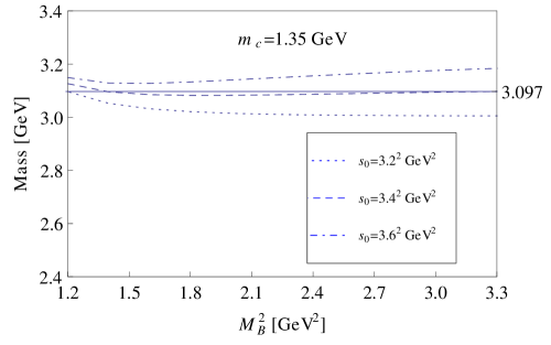
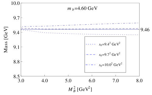
Figure 5: Running masses of the charm and bottom quarks in the Borel sum rules for $J/\psi$ and $\Upsilon(1S)$, respectively.

After performing the Borel transform, the correlation function in Eq. (II) is the function of the threshold parameter $s_{0}$ and Borel mass $M_{B}$. In the Borel sum rules analysis, there should exist suitable working regions of these two parameters in order to obtain a stable mass sum rules. For this purpose we choose the value of $s_{0}$ around which the extracted mass $m_{X}$ is stable with the variation of $M_{B}^{2}$. In Eq. (II), the exponential weight functions suppress the higher states contributions for the small value of $M_{B}^{2}$. However, the convergence of the OPE series becomes bad if $M_{B}^{2}$ is too small. These two opposite requirements restrict the domain of the Borel mass. We define the pole contribution (PC) as:

$$\text{PC}=\frac{\int_{4m_{c}^{2}}^{s_{0}}dse^{-s/M_{B}^{2}}\rho(s)}{\int_{4m_{c}^{2}}^{\infty}dse^{-s/M_{B}^{2}}\rho(s)},$$ (13)

The constraint of a relatively large pole contribution leads to the upper bound $M^{2}_{max}$ of the Borel parameter while the requirement of the OPE convergence yields the lower bound $M^{2}_{min}$.

Using the parameter values in Eq. (12), we study the tensor charmonium system by considering only $\Pi^{pert}(M_{B}^{2})$, $\Pi^{\langle G^{2}\rangle}(M_{B}^{2})$ and $\Pi^{\langle G^{3}\rangle}(M_{B}^{2})$ in Eq. (II) with $m_{1}=m_{2}=m_{c}$. The two-gluon condensate contribution is the dominant correction to the correlation function in this situation. The lower bound of the Borel parameter is obtained as $M^{2}_{min}=2.7$ GeV² by requiring that the two-gluon condensate correction be less than one fifth of the perturbative term and the tri-gluon condensate correction less than one fifth of the two-gluon condensate correction. The upper limit of $M_{B}^{2}$ is the function of $s_{0}$ as shown in Eq. (13). We choose $\sqrt{s_{0}}=4.4$ GeV around which the variation of the extracted mass $m_{X}$ with $M_{B}^{2}$ is the minimum, as shown in Fig. IIIa. Then we require that the pole contribution be larger than $50\%$ to get the upper bound of the Borel mass $M^{2}_{max}=4.0$ GeV².

By performing the numerical analysis in the domain $2.7\leq M_{B}^{2}\leq 4.0$ GeV², we obtain a stable mass sum rule of the $2^{--}$ charmonium system. The dependence of the extracted mass $m_{X}$ with the Borel parameter is very weak in this domain of $M_{B}^{2}$, as shown in Fig. IIIb. The extracted mass for the possible charmonium tensor state is about $3.97\pm 0.25$ GeV. As expected naively in the quark model, this value is slightly higher than the mass of the lowest D-wave $1^{--}$ charmonium state $\psi(3770)$.

We extend the same analysis to the $\bar{c}b$ and $\bar{b}b$ heavy quark systems and collect the numerical results in Table III. The masses of the $B_{c}$ and bottomonium tensor states are extracted to be $7.08\pm 0.34$ and $10.13\pm 0.34$ GeV, respectively. The errors are from the uncertainties of the quark masses, QCD condensates, the threshold values and the Borel parameter. The mass of the $2^{-}$ $\bar{c}b$ state was predicted to be around $7.0-7.1$ GeV in Refs. Eichten and Feinberg (1981); Gershtein et al. (1988); Chen and Kuang (1993); Eichten and Quigg (1994), which is consistent with our calculation.

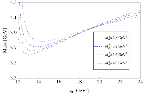
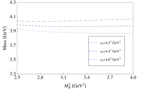
  (a)                                                                    (b)

Figure 6: Variation of $m_{X}$ with $s_{0}$(a) and $M^{2}_{B}$(b) for the $2^{--}$ charmonium state in the framework of the Borel sum rules.

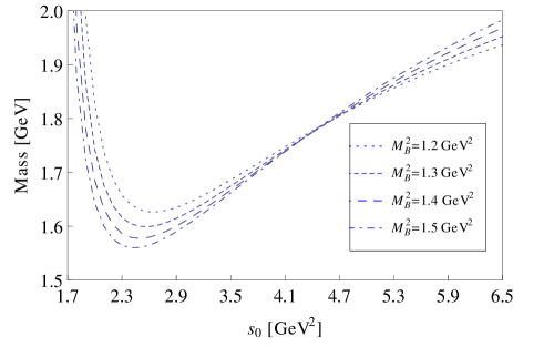
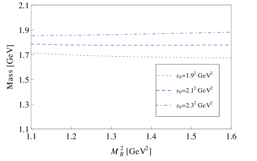
Figure 7: Variation of $m_{X}$ with $s_{0}$ and $M^{2}_{B}$ for the $2^{--}$ $\bar{q}q$ state in the framework of the Borel sum rules.

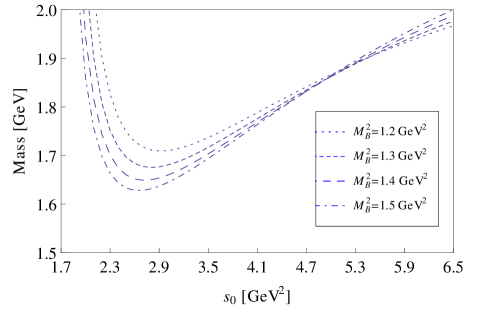
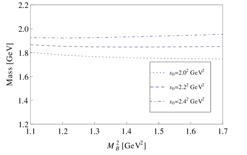
Figure 8: Variation of $m_{X}$ with $s_{0}$ and $M^{2}_{B}$ for the $2^{-}$ $\bar{q}s$ state in the framework of the Borel sum rules.

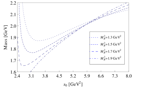
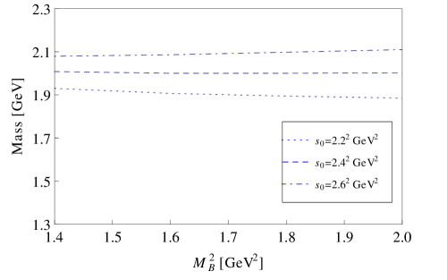
Figure 9: Variation of $m_{X}$ with $s_{0}$ and $M^{2}_{B}$ for the $2^{--}$ $\bar{s}s$ state in the framework of the Borel sum rules.

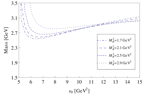
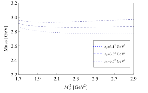
Figure 10: Variation of $m_{X}$ with $s_{0}$ and $M^{2}_{B}$ for the $2^{-}$ $\bar{q}c$ state in the framework of the Borel sum rules.

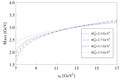
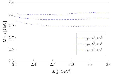
Figure 11: Variation of $m_{X}$ with $s_{0}$ and $M^{2}_{B}$ for the $2^{-}$ $\bar{s}c$ state in the framework of the Borel sum rules.

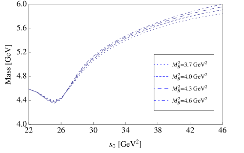
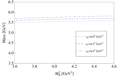
Figure 12: Variation of $m_{X}$ with $s_{0}$ and $M^{2}_{B}$ for the $2^{-}$ $\bar{q}b$ state in the framework of the Borel sum rules.

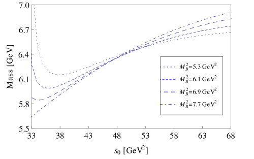
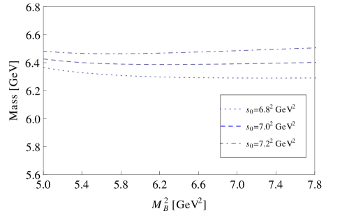
Figure 13: Variation of $m_{X}$ with $s_{0}$ and $M^{2}_{B}$ for the $2^{-}$ $\bar{s}b$ state in the framework of the Borel sum rules.

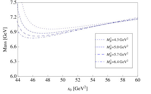
Figure 14: Variation of $m_{X}$ with $s_{0}$ and $M^{2}_{B}$ for the $2^{-}$ $\bar{c}b$ state in the framework of the Borel sum rules.

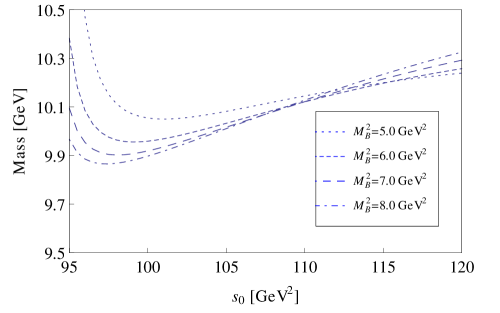
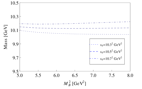
Figure 15: Variation of $m_{X}$ with $s_{0}$ and $M^{2}_{B}$ for the $2^{--}$ bottomonium state in the framework of the Borel sum rules.

We also extend the analysis to the $\bar{q}q,\bar{q}s,\bar{s}s,\bar{q}c,\bar{s}c,\bar{q}b$ and $\bar{s}b$ systems, where $q$ denotes $u$ or $d$ quark. As mentioned in Sec. II, the four quark condensate $g_{s}^{2}\langle\bar{q}_{1}q_{1}\rangle\langle\bar{q}_{2}q_{2}\rangle$ and the quark-gluon mixed condensate $\langle\bar{q}g_{s}\sigma\cdot Gq\rangle$ should be considered now. The corresponding parameters such as the quark masses and the condensates should be used for different systems in Eq. (II). Especially for the $\bar{q}c$ ($\bar{s}c$) system, only the light (strange) quark-gluon mixed condensate needs to be considered. After performing the numerical analysis, the variations of the mass with the threshold value $s_{0}$ and Borel parameter $M_{B}^{2}$ are shown in Figs. III-III. We show the Borel window, the threshold value and the extracted mass for all these systems in Table III. As shown in Table III, the light tensor meson mass is about 1.78 GeV, which is consistent with the value 1.63 GeV in Ref. Aliev and Shifman (1982).

System	$s_{0}(\mbox{GeV}^{2})$	$[M^{2}_{\mbox{min}}$,$M^{2}_{\mbox{max}}](\mbox{GeV}^{2})$	$m_{X}$(GeV)
$\bar{q}q$	$2.1^{2}$	$1.2-1.5$	$1.78\pm 0.12$
$\bar{q}s$	$2.2^{2}$	$1.2-1.6$	$1.85\pm 0.14$
$\bar{s}s$	$2.4^{2}$	$1.4-1.9$	$2.00\pm 0.16$
$\bar{q}c$	$3.3^{2}$	$1.6-2.9$	$2.86\pm 0.14$
$\bar{s}c$	$3.6^{2}$	$2.0-3.5$	$3.01\pm 0.21$
$\bar{c}c$	$4.4^{2}$	$2.7-4.0$	$3.97\pm 0.25$
$\bar{q}b$	$6.2^{2}$	$3.7-4.6$	$5.66\pm 0.33$
$\bar{s}b$	$7.0^{2}$	$4.1-7.7$	$6.40\pm 0.25$
$\bar{c}b$	$7.5^{2}$	$4.3-6.4$	$7.08\pm 0.34$
$\bar{b}b$	$10.5^{2}$	$5.0-8.0$	$10.13\pm 0.34$

Table 1: Numerical results for the various $2^{-(-)}$ tensor states in the framework of the Borel sum rules.

IV Moment sum rule analysis for $c\bar{c}$ and $b\bar{b}$ systems

For comparison, we may also use the method of the moment sum rule Shifman et al. (1979); Reinders et al. (1985) to study the $2^{--}$ charmonium and bottomonium systems. To suppress the contribution of the higher states and pick out the lowest lying resonance, we define the moment by taking derivatives of the polarization function $\Pi(q^{2})$ in Euclidean region $q^{2}=-Q^{2}<0$:

$$M_{n}(Q^{2}_{0})=\frac{1}{n!}\bigg{(}-\frac{d}{dQ^{2}}\bigg{)}^{n}\Pi(Q^{2})|_{Q^{2}=Q_{0}^{2}}=\int_{4m_{Q}^{2}}^{\infty}\frac{\rho(s)}{(s+Q^{2}_{0})^{n+1}}ds.$$ (14)

With the spectral function in Eq. 7, we obtain:

$$M_{n}(Q^{2}_{0})=\frac{f_{X}^{2}m_{X}^{6}}{(m_{X}^{2}+Q_{0}^{2})^{n+1}}\big{[}1+\delta_{n}(Q_{0}^{2})\big{]},$$ (15)

where $\delta_{n}(Q_{0}^{2})$ denotes the higher states contributions to the moment divided by the lowest lying resonance contribution. To eliminate $f_{X}$ in Eq. (15), one can consider the ratio of the moments:

$$r(n,Q_{0}^{2})\equiv\frac{M_{n}(Q_{0}^{2})}{M_{n+1}(Q_{0}^{2})}=\big{(}m_{X}^{2}+Q_{0}^{2}\big{)}\frac{1+\delta_{n}(Q_{0}^{2})}{1+\delta_{n+1}(Q_{0}^{2})}.$$ (16)

From the ratio $r(n,Q_{0}^{2})$ one can immediately extract the mass of the lowest lying resonance $m_{X}$ for $\delta_{n}(Q_{0}^{2})\cong\delta_{n+1}(Q_{0}^{2})$ at sufficiently high $n$.

However, taking higher derivative $n$ means moving further away from the asymptotically free region. This can be compensated by choosing a larger $Q_{0}^{2}$. In Eq. (16), it will be difficult to extract the mass of the lowest lying resonance for large value of $Q_{0}^{2}$ because $\delta_{n}(Q_{0}^{2})$ converges less fast in this situation. In fact, one can arrive a region in the $(n,Q_{0}^{2})$ plane where the lowest lying resonance dominates the integral in Eq. (14) and the nonperturbative contribution is not too large. The moment $M_{n}(Q^{2})$ can be drawn from the Borel transformed correlation function shown in Sec. II after taking into account the gluon condensate and tri-gluon condensate.

Using the QCD condensates in Eq. (12) and the heavy quark masses extracted in Fig. III, we perform numerical analysis to obtain the $c\bar{c}$ and $b\bar{b}$ hadron masses as the function of $Q_{0}^{2}$ and $n$. In Fig. IV, we show the masses of the $2^{--}$ charmonium and bottomonium states as the function of $n$. There is a mass minimum in these curves under the variation with $n$. By choosing $Q_{0}^{2}=50m_{c}^{2},60m_{c}^{2},70m_{c}^{2}$ for the charmonium system and $Q_{0}^{2}=4m_{b}^{2},8m_{b}^{2},12m_{b}^{2}$ for the bottomonium system, the extracted mass converges to $m_{X_{c\bar{c}}}=(4.13\pm 0.20)$ GeV and $m_{X_{b\bar{b}}}=(10.27\pm 0.39)$ GeV respectively. These values are consistent with the results of the Borel sum rules within the errors.

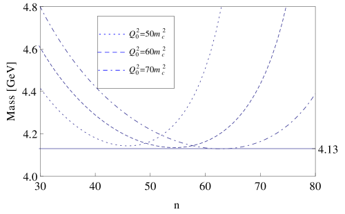
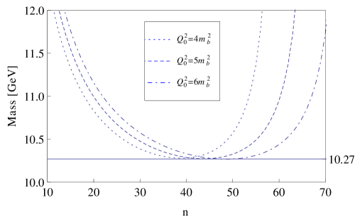
Figure 16: Variation of $m_{X}$ with $n$ for the charmonium and bottomonium states in the framework of the moment sum rules.

V Summary

We have shown that the interpolating tensor current in Eq. (2) is the correct operator for the $J^{PC}=2^{--}$ meson, the $J_{ij}$ and $J_{0i}$ components of which reduce to the D-wave and P-wave states respectively in the non-relativistic limit in terms of the quark model picture as shown in the appendix. Then we make the operator product expansion (OPE) and calculate the two-point correlation function. For the heavy quark $\bar{Q}_{1}Q_{2}$ ($Q_{1},Q_{2}=c,b$) systems, the power corrections include the gluon condensate $\langle g_{s}^{2}GG\rangle$ and the tri-gluon condensate $\langle g_{s}^{3}fGGG\rangle$ only. For the light quarks systems and the light-heavy quarks systems, the four quark condensate $g_{s}^{2}\langle\bar{q}_{1}q_{1}\rangle\langle\bar{q}_{2}q_{2}\rangle$ (only for the light quarks systems) and the quark-gluon mixed condensate $\langle\bar{q}g_{s}\sigma\cdot Gq\rangle$ also contribute to the sum rules. While the gluon condensate $\langle g_{s}^{2}GG\rangle$ is the dominant nonperturbative correction for the above systems, these terms also play an important role in the tensor meson sum rules.

Within the framework of the Borel sum rules, we have studied the $\bar{q}q,\bar{q}s,\bar{q}c,\bar{s}c,\bar{c}c,\bar{q}b,\bar{s}b,\bar{c}b$ and $\bar{b}b$ systems. All these systems display stable QCD sum rules in the working regions of the Borel parameter $M_{B}^{2}$. Up to now, none of these $2^{-}$ tensor mesons have been observed except the strange meson $K_{2}(1770)$ and $K_{2}(1820)$  Nakamura et al. (2010). As shown in Table. III, the extracted mass of the $\bar{q}s$ tensor state is about 1.85 GeV, which is consistent with the mass of the strange mesons $K_{2}(1770)$ and $K_{2}(1820)$  Nakamura et al. (2010). The lowest D-wave charmonium state is $\psi(3770)$ with $J^{PC}=1^{--}$. The extracted mass of the $2^{--}$ D-wave charmonium state is around $3.97$ GeV, which is slightly higher than $\psi(3770)$ as expected in the quark model. For the charmonium and bottomonium systems, we also perform the moment sum rules analysis for comparison. Hopefully the present investigation will be helpful to the future experimental search of these tensor states.

Appendix A THE QUANTUM NUMBERS OF THE INTERPOLATING CURRENT

In order to study the quantum numbers of the tensor current in Eq. (2), we perform the parity transformation and charge conjugation transformation to $J_{\mu\nu}$:

$$\mathbb{P}J_{\mu\nu}\mathbb{P}^{-1} =-(-1)^{\mu}(-1)^{\nu}J_{\mu\nu}$$

$$\mathbb{C}J_{\mu\nu}\mathbb{C}^{-1} =-J_{\mu\nu}$$ (17)

where $(-1)^{\mu}=1$ for $\mu=0$ and $(-1)^{\mu}=-1$ for $\mu=1,2,3$. With these relations and the trace condition in Eq. (3), the tensor current can couple to the $1^{+-}$ ($J_{0i}$ components, i=1,2,3) and $2^{--}$ ($J_{ij}$ components) states at the same time.

It’s interesting to reduce this operator in the non-relativistic limit and center of mass frame in terms of the quark model language.

$$J_{ij}(x) = \bar{Q}_{1}(x)\gamma_{i}\gamma_{5}\overleftrightarrow{\partial_{j}}Q_{2}(x)+(i\leftrightarrow j)$$ (18)

$$\sim \bar{u}(p^{\prime},s)\gamma_{i}\gamma_{5}ik_{j}v(p,r)+(i\leftrightarrow j)=-\frac{1}{2m}\varphi_{s}^{{\dagger}}\epsilon_{ikl}\sigma_{l}k_{k}k_{j}\chi_{r}+(i\leftrightarrow j)$$

$$J_{0i}(x) = \bar{Q}_{1}(x)(\gamma_{0}\gamma_{5}\overleftrightarrow{\partial_{i}}+\gamma_{i}\gamma_{5}\overleftrightarrow{\partial_{0}})Q_{2}(x)$$ (19)

$$\sim \bar{u}(p^{\prime},s)\gamma_{0}\gamma_{5}ik_{i}v(p,r)=ik_{i}\varphi_{s}^{{\dagger}}\chi_{r}$$

$$J_{00}(x) \sim ik_{0}\varphi_{s}^{{\dagger}}\chi_{r}=0$$ (20)

in which $k=p-p^{\prime}$ and ${\vec{q}}={\vec{p}}+{\vec{p}}^{\prime}=0$ in the center of mass system. We have used the non-relativistic limit: $E_{p^{\prime}}=E_{p}=m,k_{0}=0$. It is obvious that $J_{ij}$ reduces to the D-wave and $J_{0i}$ reduces to P-wave in the non-relativistic limit. Therefore the quantum numbers of the current should be $2^{--}$ for the $J_{ij}$ component and $1^{+-}$ for the $J_{0i}$ component.

Appendix B THE MOMENTUM SPACE PROPAGATOR

To calculate the higher dimensional gluonic operators, we consider the gluon field as an external one with the fixed-point gauge condition Dubovikov and Smilga (1981); Cronstrom (1980); Shifman (1980):

$$(x-x_{0})^{\mu}A_{\mu}^{a}(x)=0,$$ (21)

where $x_{0}$ is an arbitrary point in space which can be chosen to be the origin. Then the four potential $A_{\mu}^{a}$ can be expressed in terms of the field strength tensor $G_{\mu\nu}$($G_{\mu\nu}=\frac{\lambda^{a}}{2}G_{\mu\nu}^{a}$):

$$A_{\mu}(x) =\int_{0}^{1}tdtG_{\nu\mu}(tx)x^{\nu}$$

$$=\frac{1}{2}x^{\nu}G_{\nu\mu}(0)+\frac{1}{3}x^{\alpha}x^{\nu}D_{\alpha}G_{\nu\mu}(0)+\frac{1}{8}x^{\alpha}x^{\beta}x^{\nu}D_{\alpha}D_{\beta}G_{\nu\mu}(0)+...,$$

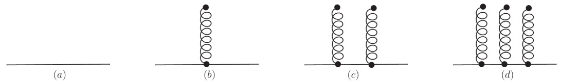
Figure 17: Graphic representations of the massive quark propagators with gluon legs attached to the quark line.

Denote the massive quark propagator between the position $x$ and $y$ in the coordinate space as $iS_{0}(x,y)$. The massive quark propagator in the momentum space can be obtained as:

$$iS(p) =iS_{0}(p)+iS_{g}(p)+iS_{gg}(p)+iS_{ggg}(p),$$ (22)

where $iS_{0}(p)$ is the free quark propagator as shown in Fig. B(a):

$$iS_{0}(p)=\frac{i}{\hat{p}-m},$$ (23)

$iS_{g}(p)$ is the quark propagator with one gluon leg attached as shown in Fig B(b):

$$iS_{g}(p)=\frac{i}{4}\frac{\lambda^{n}}{2}g_{s}G^{n}_{\mu\nu}\frac{\sigma^{\mu\nu}(\hat{p}+m)+(\hat{p}+m)\sigma^{\mu\nu}}{(p^{2}-m^{2})^{2}}+\frac{i}{2}\frac{\lambda^{n}}{2}g_{s}G^{n}_{\mu\nu}\bigg{[}\frac{2y^{\mu}p^{\nu}(\hat{p}+m)}{(p^{2}-m^{2})^{2}}-\frac{y^{\mu}\gamma^{\nu}}{p^{2}-m^{2}}\bigg{]}$$ (24)

$iS_{gg}(p)$ is the quark propagator with two gluon legs attached as shown in Fig B(c):

$$iS_{gg}(p) = -\frac{i}{4}\frac{\lambda^{a}}{2}\frac{\lambda^{b}}{2}g^{2}_{s}G^{a}_{\mu\rho}G^{b}_{\nu\sigma}\frac{\hat{p}+m}{(p^{2}-m^{2})^{5}}\big{(}f^{\mu\rho\nu\sigma}+f^{\mu\nu\rho\sigma}+f^{\mu\nu\sigma\rho}\big{)}$$ (25)

$$-\frac{1}{4}\frac{\lambda^{a}}{2}\frac{\lambda^{b}}{2}g^{2}_{s}G^{a}_{\mu\rho}G^{b}_{\nu\sigma}\frac{\hat{p}+m}{(p^{2}-m^{2})^{4}}\Big{[}y^{\sigma}(f^{\mu\rho\nu}+f^{\mu\nu\rho})+y^{\rho}f^{\mu\nu\sigma}-iy^{\rho}y^{\sigma}f^{\mu\nu}(p^{2}-m^{2})\Big{]}$$

$iS_{ggg}(p)$ is the quark propagator with three gluon legs attached as shown in Fig B(d):

$$iS_{ggg}(p) = \frac{i}{8}\frac{\lambda^{a}}{2}\frac{\lambda^{b}}{2}\frac{\lambda^{c}}{2}g_{s}^{3}G^{a}_{\mu\alpha}G^{b}_{\nu\beta}G^{c}_{\rho\gamma}\frac{\hat{p}+m}{(p^{2}-m^{2})^{7}}\big{(}f^{\mu\alpha\nu\beta\rho\gamma}+f^{\mu\alpha\nu\rho\beta\gamma}+f^{\mu\alpha\nu\rho\gamma\beta}+f^{\mu\nu\alpha\beta\rho\gamma}+f^{\mu\nu\beta\alpha\rho\gamma}+f^{\mu\nu\beta\rho\alpha\gamma}$$ (26)

$$+f^{\mu\nu\beta\rho\gamma\alpha}+f^{\mu\nu\alpha\rho\beta\gamma}+f^{\mu\nu\alpha\rho\gamma\beta}+f^{\mu\nu\rho\alpha\beta\gamma}+f^{\mu\nu\rho\beta\alpha\gamma}+f^{\mu\nu\rho\beta\gamma\alpha}+f^{\mu\nu\rho\alpha\gamma\beta}+f^{\mu\nu\rho\gamma\alpha\beta}+f^{\mu\nu\rho\gamma\beta\alpha}\big{)}$$

$$-\frac{i}{8}\frac{\lambda^{a}}{2}\frac{\lambda^{b}}{2}\frac{\lambda^{c}}{2}g_{s}^{3}G^{a}_{\mu\alpha}G^{b}_{\nu\beta}G^{c}_{\rho\gamma}\frac{\hat{p}+m}{(p^{2}-m^{2})^{6}}\bigg{\{}\Big{[}iy^{\alpha}(f^{\mu\nu\beta\rho\gamma}+f^{\mu\nu\rho\beta\gamma}+f^{\mu\nu\rho\gamma\beta})+iy^{\beta}(f^{\mu\alpha\nu\rho\gamma}+f^{\mu\nu\alpha\rho\gamma}$$

$$+f^{\mu\nu\rho\gamma\alpha}+f^{\mu\nu\rho\alpha\gamma})+iy^{\gamma}(f^{\mu\alpha\nu\beta\rho}+f^{\mu\alpha\nu\rho\beta}+f^{\mu\nu\alpha\beta\rho}+f^{\mu\nu\beta\alpha\rho}+f^{\mu\nu\beta\rho\alpha}+f^{\mu\nu\alpha\rho\beta}+f^{\mu\nu\rho\alpha\beta}+f^{\mu\nu\rho\beta\alpha})\Big{]}$$

$$+(p^{2}-m^{2})\Big{[}y^{\alpha}y^{\beta}f^{\mu\nu\rho\gamma}+y^{\alpha}y^{\gamma}(f^{\mu\nu\beta\rho}+f^{\mu\nu\rho\beta})+y^{\beta}y^{\gamma}(f^{\mu\alpha\nu\rho}+f^{\mu\nu\alpha\rho}+f^{\mu\nu\rho\alpha})\Big{]}$$

$$-iy^{\alpha}y^{\beta}y^{\gamma}f^{\mu\nu\rho}(p^{2}-m^{2})^{2}\bigg{\}}$$

where $f^{\mu\nu...\alpha\beta}=\gamma^{\mu}(p^{2}-m^{2})\gamma^{\nu}(p^{2}-m^{2})...\gamma^{\alpha}(p^{2}-m^{2})\gamma^{\beta}(p^{2}-m^{2})$.

References

- Brambilla et al. (2004) N. Brambilla et al. (Quarkonium Working Group) (2004), eprint hep-ph/0412158.
- Swanson (2006) E. S. Swanson, Phys. Rept. 429, 243 (2006), eprint hep-ph/0601110.
- Zhu (2008) S.-L. Zhu, Int. J. Mod. Phys. E17, 283 (2008), eprint hep-ph/0703225.
- Bracko (2009) M. Bracko (2009), eprint 0907.1358.
- Yuan (2009) C.-Z. Yuan (Belle) (2009), eprint 0910.3138.
- Rosner (2007) J. L. Rosner, J. Phys. Conf. Ser. 69, 012002 (2007), eprint hep-ph/0612332.
- Choi et al. (2008) S. K. Choi et al. (BELLE), Phys. Rev. Lett. 100, 142001 (2008), eprint 0708.1790.
- Rosner et al. (2005) J. L. Rosner et al. (CLEO), Phys. Rev. Lett. 95, 102003 (2005), eprint hep-ex/0505073.
- Nakamura et al. (2010) K. Nakamura et al. (Particle Data Group), J. Phys. G37, 075021 (2010).
- Dudek et al. (2008) J. J. Dudek, R. G. Edwards, N. Mathur, and D. G. Richards, Phys. Rev. D77, 034501 (2008), eprint 0707.4162.
- Aliev et al. (2010) T. M. Aliev, K. Azizi, and M. Savci, Phys. Lett. B690, 164 (2010), eprint 1002.2767.
- Wei et al. (2006) W. Wei, L. Zhang, and S.-L. Zhu, Int. J. Mod. Phys. A21, 4617 (2006), eprint hep-ph/0411140.
- Reinders et al. (1982) L. J. Reinders, S. Yazaki, and H. R. Rubinstein, Nucl. Phys. B196, 125 (1982).
- Aliev and Shifman (1982) T. M. Aliev and M. A. Shifman, Phys. Lett. B112, 401 (1982).
- Shifman et al. (1979) M. A. Shifman, A. I. Vainshtein, and V. I. Zakharov, Nucl. Phys. B147, 385 (1979).
- Reinders et al. (1985) L. J. Reinders, H. Rubinstein, and S. Yazaki, Phys. Rept. 127, 1 (1985).
- Colangelo (2000) P. Colangelo, and A. Khodjamirian, Frontier of Particle Physics 3* (2000), eprint hep-ph/0010175.
- Jamin et al. (2002) M. Jamin, J. A. Oller, and A. Pich, Eur. Phys. J. C24, 237 (2002), eprint hep-ph/0110194.
- Dominguez et al. (1994) C. A. Dominguez, G. R. Gluckman, and N. Paver, Phys. Lett. B333, 184 (1994), eprint hep-ph/9406329.
- Narison (1994) S. Narison, Phys. Lett. B341, 73 (1994), eprint hep-ph/9408376.
- Eidemuller and Jamin (2001) M. Eidemuller and M. Jamin, Phys. Lett. B498, 203 (2001), eprint hep-ph/0010334.
- Kuhn and Steinhauser (2001) J. H. Kuhn and M. Steinhauser, Nucl. Phys. B619, 588 (2001), eprint hep-ph/0109084.
- Ioffe and Zyablyuk (2003) B. L. Ioffe and K. N. Zyablyuk, Eur. Phys. J. C27, 229 (2003), eprint hep-ph/0207183.
- Chetyrkin et al. (2009) K. G. Chetyrkin et al., Phys. Rev. D80, 074010 (2009), eprint 0907.2110.
- Eichten and Feinberg (1981) E. Eichten and F. Feinberg, Phys. Rev. D23, 2724 (1981).
- Gershtein et al. (1988) S. S. Gershtein, V. V. Kiselev, A. K. Likhoded, S. R. Slabospitsky, and A. V. Tkabladze, Sov. J. Nucl. Phys. 48, 327 (1988).
- Chen and Kuang (1993) Y.-Q. Chen and Y.-P. Kuang, Phys. Rev. D47, 350 (1993).
- Eichten and Quigg (1994) E. J. Eichten and C. Quigg, Phys. Rev. D49, 5845 (1994), eprint hep-ph/9402210.
- Dubovikov and Smilga (1981) M. S. Dubovikov and A. V. Smilga, Nucl. Phys. B185, 109 (1981).
- Cronstrom (1980) C. Cronstrom, Phys. Lett. B90, 267 (1980).
- Shifman (1980) M. A. Shifman, Nucl. Phys. B173, 13 (1980).