Lie-Algebraic Interpretation of the Maximal Superintegrability and Exact Solvability of the Coulomb-Rosochatius Potential in $n$ Dimensions

Abstract

The potential group method is applied to the $n$-dimensional Coulomb-Rosochatius potential, whose bound states and scattering states are worked out in detail. As far as scattering is concerned, the $S$-matrix elements are computed by the method of intertwining operators and an integral representation is obtained for the scattering amplitude. It is shown that the maximal superintegrability of the system is due to the underlying potential group and that the $2n-1$ integral of motions are related to Casimir operators of subgroups.

1 Introduction

The Coulomb system in arbitrary dimensions is among the well-known and best studied exactly solvable systems in quantum mechanics[1]-[13]. It describes the dynamics of charged particles under the influence of the $1/r$  potential. This is what we conventionally mean by Coulomb system, even if the true $n$-dimensional Coulomb potential satisfying the Poisson equation goes like $1/r^{n-2}$, for $n\geq 3$.

It has been shown that the bound and scattering states of a Coulomb system in $n$ dimensions can be associated with the rotation group $SO\left(n+1\right)$ and the Lorentz group $SO\left(n,1\right),$ respectively[1]-[4]. In other words, for a fixed energy, these groups appear as invariance groups of the system. These symmetries for $n=3$ were discovered by Fock[14] and Bargmann[15]. Moreover, it was pointed out in Ref.[7] that the dynamical group that yields the positive and negative energy spectra of the Coulomb problem in $n$ dimensions is $SO\left(2,n+1\right)$,  while the dynamical group in the case $n=3$ had been discussed by Barut[16]. It is also worth noting that Coulomb and harmonic-oscillator systems are the only spherically symmetric superintegrable systems in arbitrary dimensions.

We recall that in classical mechanics a closed system with $n$ degrees of freedom is completely integrable if it admits $n$ integrals of motion (including the Hamiltonian ) that are independent and in involution , i.e. the Poisson brackets of any two integrals are zero. The system is called superintegrable if there exist $q$, $1\leq q\leq n-1$, additional independent integrals of motion. The cases $q=1$ and $q=n-1$ correspond to minimal and maximal superintegrability, respectively. In quantum mechanics the definitions of complete integrability and superintegrability are same, but Poisson brackets are replaced by commutators (see Ref.[17] for a general review).

In the present work we shall consider a quantum system characterized by a Hamiltonian of the form

$$H=\frac{1}{2}p^{2}-\frac{\alpha}{r}+\sum_{i=1}^{n}\frac{\beta_{i}}{2x_{i}^{2}}\qquad.$$ (1)

We shall call the system governed by the Hamiltonian given above the Coulomb-Rosochatius[18] system.The motion is confined to the region bounded by the singularity of $H$ at hyper-planes $x_{i}=0,\ i=1,2,\ldots,n$ , i.e. hyper-octant ( one of the $2^{n}$ regions of Euclidean space $E^{n}$). Without loss of generality this can be taken to be the non-negative hyper-octant ( i.e. where $x_{i}\geq 0,\ i=1,2,\ldots,n$ ).

The main interest of the Coulomb-Rosochatius system consists in its maximal superintegrability, recently proved for $n=3$ in the classical case[19] (see also [20]). The system had been proved long ago [21],[22] to be quasi-maximally superintegrable for $n\leq 3$, i.e. to admit $2n-2$ operators quadratic in the momenta. For $n=3$, the fifth integral of motion quartic in the momenta was explicitly worked out in Refs[19]-[20], thus proving the maximal superintegrability of the classical Coulomb-Rosochatius system. Finally, the maximal superintegrability of the classical system (1) in $n$-dimensional spherical, hyperbolic and Euclidean spaces was proved in Ref.[23]: here again, one of the $2n-1$ functionally independent integrals of motion turns out to be quartic in the momenta, while the remaining ones are quadratic.

The main purpose of the present work is the complete algebraic solution of bound states and scattering states of the quantum-mechanical Coulomb-Rosochatius system in $n$ dimensions and the derivation of the $2n-1$ integrals of motion expected for maximal superintegrability.

Before describing the method of solution of the quantum Coulomb-Rosochatius system in $n$ dimensions , a few definitions are in order: a Lie group $G$ is an invariance group for a quantum-mechanical system with Hamiltonian $H$ if the latter can be related to a suitable function of a Casimir operator, $C$, of the group, $G$

$$H=f\left(C\right)\;.$$ (2)

An algebraic derivation of the energy spectrum is possible also when

$$H=f\left(C\right)|_{\mathcal{H}}.$$ (3)

where $\mathcal{H}$ is a subspace of the carrier space. In this case the group $G$ describes the same energy states of a family of Hamiltonians $H$ with different potential strength. This is why $G$ is called potential group [24]. Such an approach was proposed by Ghirardi [25], who worked it out in detail for the Scarf potential [26]. It is similar to the approach of Olshanetsky and Perelomov [27, 28], where quantum integrable systems are related to the radial part of the Laplace operator on homogeneous spaces,i.e. to the radial part of a second-order Casimir operator of a Lie group. Moreover, it has been shown in Ref. [29] that the $S$ matrix  can be associated with an intertwining operator, $A$, between two Weyl-equivalent representations, $U^{\chi}$ and $U^{\widetilde{\chi}}$, of $G$, i.e. two representations with the same Casimir eigenvalues.

By definition, $A$ satisfies the following equations

$$AU^{\chi}\left(g\right)=U^{\widetilde{\chi}}\left(g\right)A\;,\;\forall\;g\;\epsilon\;G$$ (4)

and

$$AdU^{\chi}\left(b\right)=dU^{\widetilde{\chi}}\left(b\right)\;,\;\ \forall\;b\;\epsilon\;\mathfrak{g}$$ (5)

where $dU^{\chi}$ and $dU^{\widetilde{\chi}}$ are the corresponding representations of the algebra, $\mathfrak{g}$, of $G$. Eqs. (4-5) have high restrictive power, determining the intertwining operator up to a constant. The $S$ matrix coincides with the intertwining operator $A$

$$S=A$$ (6)

if eq. (2) holds, and with the reduction of $A$ to a proper Hilbert subspace $\mathcal{H}$

$$S=A|_{\mathcal{H}}$$ (7)

if eq. (3) holds.

The plan of the paper is as follows: Section 2 will describe in full detail the potential group for the Coulomb-Rosochatius system, with a potential specialized to

$$V(r)=-\frac{\gamma}{r}+\sum_{i=1}^{n}\frac{\kappa_{i}\left(\kappa_{i}+1\right)}{x_{i}^{2}},$$ (8)

with Subsection 2.1 dedicated to the derivation of bound states and Subsection 2.2 to scattering states. Finally, Section 3 will be devoted to conclusions and perspectives.

2 Potential group for the Coulomb-Rosochatius system

It is well known that the group $SO\left(N+1\right)$ ( $SO\left(N,1\right)$ ) has a class of unitary irreducible representations (UIR’s) characterized by a number $j,\ j=0,1,2,\ldots$ ($j=-\frac{N-1}{2}+i\rho,\ \rho>0$) in which the basis vectors are completely labelled by $N-1$ numbers only. This representation can be realized in the Hilbert space spanned by negative-energy (positive-energy) states corresponding to a fixed eigenvalue of the Coulomb Hamiltonian in $N$ dimensions. According to this, one introduces the angular momentum operators $L_{ij}$ and the $N$-dimensional Runge-Lenz vector $A_{i}$

$$L_{ij}=\zeta_{i}\pi_{j}-\zeta_{j}\pi_{i}\;,\;\left(i,j=1,...,N\right)$$ (9)

and

$$A_{i} = -\frac{1}{2}\sum_{j=1}^{N}\left(L_{ij}\pi_{j}+\pi_{j}L_{ij}\right)+\frac{\gamma\zeta_{i}}{\sqrt{\zeta^{2}}}\;$$ (10)

$$= \left(\zeta\cdot\pi\right)\pi_{i}-\zeta_{i}\pi^{2}-i\frac{N-1}{2}\pi_{i}+\frac{\gamma\zeta_{i}}{\sqrt{\zeta^{2}}},\;(i=1,...,N)$$

respectively, where $\zeta=\left(\zeta_{1},\zeta_{2},\ldots,\zeta_{N}\right)$, $\ \ \pi=\left(\ \pi_{1},\pi_{2},\ldots,\pi_{N}\right),\ \pi_{j}=-i\frac{\partial}{\partial\zeta_{j}}$, , $\zeta^{2}=\sum_{i=1}^{N}\zeta_{i}^{2}$, $\pi^{2}=\sum_{i=1}^{N}\pi_{i}^{2}$. These operators satisfy the following commutation relations

$$\left[L_{ij},L_{kl}\right]={\normalsize i}\left({\normalsize\delta}_{ik}L_{jl}+{\normalsize\delta}_{jl}L_{ik}-{\normalsize\delta}_{il}L_{jk}-{\normalsize\delta}_{jk}L_{il}\right)$$

$$\left[L_{ij},A_{k}\right]={\normalsize i}\left({\normalsize\delta}_{ik}A_{j}-{\normalsize\delta}_{jk}A_{i}\right)$$ (11)

$$\left[A_{i},A_{j}\right]=-{\normalsize i}2hL_{ij}\;,$$

where $h$ is the Coulomb Hamiltonian in $N$ dimensions

$$h=\frac{1}{2}\pi^{2}-\frac{\gamma}{\sqrt{\zeta^{2}}}.$$ (12)

Since $\left[L_{ij},h\right]=\left[A_{i},h\right]=0$ , we may restrict the above algebra to a subspace where $h$ has a definite eigenvalue $\varepsilon$ and define a new set of operators as follows

$$M_{i,0} = -M_{0,i}=\left|2\varepsilon\right|^{-\frac{1}{2}}A_{i}\;,\;(i=1,...,N)$$

$$M_{ij} = L_{ij}\;,\;\left(i,j=1,...,N\right).$$ (13)

Then, as a result, we obtain the Lie algebra of $SO\left(N+1\right)$ (when $\varepsilon$ is negative) and the Lie algebra of $SO\left(N,1\right)$ (when $\varepsilon$ is positive)

$$\left[M_{\mu\nu},M_{\sigma\lambda}\right]={\normalsize i}\left(g_{\mu\sigma}M_{\nu\lambda}+g_{\nu\lambda}M_{\mu\sigma}-g_{\mu\lambda}M_{\nu\sigma}-g_{\nu\sigma}M_{\mu\lambda}\right)\;,$$ (14)

where $\mu,\nu=0,1,2,...,N$ and

$$g_{\mu\nu} = \left(+,+,\ldots,+,+\right)\quad\textstyle{for\ \ }SO\left(N+1\right)$$ (15)

$$g_{\mu\nu} = \left(-,+,\ldots,+,+\right)\quad\textstyle{for\ \ }SO\left(N,1\right)$$

The generators $M_{\mu\nu}$ act in the eigenspace $\mathcal{H}$ of $h$ equipped with the scalar product

$$\left(\phi_{1},\phi_{2}\right)=\int\limits_{R^{N}}\phi_{1}^{\ast}\left(\zeta\right)\phi_{2}\left(\zeta\right)d\zeta,\quad\zeta\in R^{N}$$ (16)

where $d\zeta=d\zeta_{1}d\zeta_{2}\cdots d\zeta_{N}$. A detailed discussion of the $SO\left(N+1\right)$ ($SO\left(N,1\right)$) representation  generated by operators (13) is given in Refs.[1]-[4].

At this stage we note that, in  general, one can define the generators of $SO\left(N+1\right)$ ( $SO\left(N,1\right)$ ) (let us call them $\tilde{M}_{\mu\nu}$), as follows

$$\tilde{M}_{i,0} = -\tilde{M}_{0,i}=\left|2\varepsilon\right|^{-\frac{1}{2}}\lambda^{1/2}\left(\zeta\right)\circ A_{i}\circ\lambda^{-1/2}\left(\zeta\right)$$

$$\tilde{M}_{ij} = \lambda^{1/2}\left(\zeta\right)\circ L_{ij}\circ\lambda^{-1/2}\left(\zeta\right)$$

where $\lambda$ is some non-negative function of $\ \zeta$. Now the generators $\tilde{M}_{\mu\nu}$ act in the eigenspace $\tilde{\mathcal{H}}$ of $\tilde{h}=\lambda^{1/2}\left(\zeta\right)\circ h\circ\lambda^{-1/2}\left(\zeta\right)$ equipped with the scalar product

$$\left(\tilde{\phi}_{1},\tilde{\phi}_{2}\right)=\int\limits_{R^{N}}\tilde{\phi}_{1}^{\ast}\left(\zeta\right)\tilde{\phi}_{2}\left(\zeta\right)d\mu\left(\zeta\right),\quad\zeta\in R^{N}$$ (17)

where $d\mu\left(\zeta\right)=\lambda^{-1}\left(\zeta\right)d\zeta$ is a quasi-invariant measure on  $R^{N}$. The representations acting in $\mathcal{H}$ and $\tilde{\mathcal{H}}$ are, of course, unitarily equivalent. The unitary mapping $W$ which realizes the equivalence is given by

$$W:\textstyle{\ \ \ \ }\phi\rightarrow\tilde{\phi}=\lambda^{1/2}\left(\zeta\right)\phi$$ (18)

Although these representations are equivalent from the mathematical view-point, they may be related to different physical problems. We shall prove that the bound states and scattering states of the quantum system (8) are related to the representation of $SO(3n+1)$ and $SO(3n,1)$ , respectively, acting in the Hilbert space with scalar product

$$\left(\tilde{\phi}_{1},\tilde{\phi}_{2}\right)=\int\limits_{R^{3n}}\tilde{\phi}_{1}^{\ast}\left(\zeta\right)\tilde{\phi}_{2}\left(\zeta\right)d\mu\left(\zeta\right),$$ (19)

where $d\mu\left(\zeta\right)=\prod_{i=1}^{n}\left(\zeta_{3i-2}^{2}+\zeta_{3i-1}^{2}+\zeta_{3i}^{2}\right)^{-1}d\zeta$. To this end, we choose $N=3n$ and $\lambda\left(\zeta\right)=\prod_{i=1}^{n}\left(\zeta_{3i-2}^{2}+\zeta_{3i-1}^{2}+\zeta_{3i}^{2}\right)$. Then we introduce the second-order Casimir operator

$$\tilde{C}=\frac{1}{2}\sum\limits_{\mu,\nu=0}^{3n}\tilde{M}^{\mu\nu}\tilde{M}_{\mu\nu}$$ (20)

and consider the following operator depending on $\tilde{C}$

$$\frac{\gamma^{2}}{\left[\tilde{C}+\left(\frac{3n-1}{2}\right)^{2}\right]}$$

$$= \frac{\partial^{2}}{\partial\zeta_{1}^{2}}+\ldots+\frac{\partial^{2}}{\partial\zeta_{3n}^{2}}-\frac{2}{\zeta_{1}^{2}+\zeta_{2}^{2}+\zeta_{3}^{2}}\left(\zeta_{1}\frac{\partial}{\partial\zeta_{1}}+\zeta_{2}\frac{\partial}{\partial\zeta_{2}}+\zeta_{3}\frac{\partial}{\partial\zeta_{3}}\right)$$

$$-\cdots-\frac{2}{\zeta_{3n-2}^{2}+\zeta_{3n-1}^{2}+\zeta_{3n}^{2}}\left(\zeta_{3n-2}\frac{\partial}{\partial\zeta_{3n-2}}+\zeta_{3n-1}\frac{\partial}{\partial\zeta_{3n-1}}+\zeta_{3n}\frac{\partial}{\partial\zeta_{3n}}\right)+\frac{2\gamma}{\sqrt{\zeta^{2}}}$$

Decomposing $R^{3n}$ into the direct sum of three-dimensional subspaces and introducing spherical coordinates in these subspaces

$$\zeta=\left(x_{1}u_{1},x_{2}u_{2},\ldots,x_{n}u_{n}\right)$$ (21)

where $u_{i}=\left(\sin\alpha_{i}\sin\beta_{i},\sin\alpha_{i}\cos\beta_{i},\cos\alpha_{i}\right),\ x_{i}\geq 0,\ 0\leq\alpha_{i}\leq\pi,\ 0\leq\beta_{i}\leq 2\pi,\ (i=1,2,\ldots,n)$ , we have

$$\frac{\gamma^{2}}{\left[\tilde{C}+\left(\frac{3n-1}{2}\right)^{2}\right]}$$

$$= \sum_{i=1}^{n}\left[\frac{\partial^{2}}{\partial x_{i}^{2}}+\frac{1}{x_{i}^{2}}\left(\frac{1}{\sin\alpha_{i}}\frac{\partial}{\partial\alpha_{i}}\sin\alpha_{i}\frac{\partial}{\partial\alpha_{i}}+\frac{1}{\sin^{2}\alpha_{i}}\frac{\partial^{2}}{\partial\beta_{i}^{2}}\right)\right]+\frac{2\gamma}{\sqrt{x^{2}}}$$

with $x=\left(x_{1},x_{2},\ldots,x_{n}\right).$ With this coordinate system the measure $d\mu\left(\zeta\right)$ in formula (19) becomes $d\mu\left(\zeta\right)=dx\prod_{i=1}^{n}\sin\alpha_{i}d\alpha_{i}d\beta_{i}$, where $dx=dx_{1}dx_{2}\cdots dx_{n}.$

Let $\mathcal{H}_{K}$, $K=\left(\kappa_{1},\kappa_{2},\ldots,\kappa_{n};\sigma_{1},\sigma_{2},\ldots,\sigma_{n}\right)$, be a subspace of functions $\hat{\phi}\left(\zeta\right)=\Psi\left(x\right)\prod_{i=1}^{n}Y_{\kappa_{i}}^{\sigma_{i}}\left(\alpha_{i},\beta_{i}\right),$ with fixed $K$, where $Y_{\kappa_{i}}^{\sigma_{i}}\left(\alpha_{i},\beta_{i}\right)$ are spherical harmonics of degree $\kappa_{i}$. Thus, the operator (2) restricted to this subspace becomes

$$\left.\frac{\gamma^{2}}{\left[\tilde{C}+\left(\frac{3n-1}{2}\right)^{2}\right]}\right|_{\mathcal{H}_{K}}=\sum_{i=1}^{n}\left[\frac{\partial^{2}}{\partial x_{i}^{2}}-\frac{\kappa_{i}\left(\kappa_{i}+1\right)}{x_{i}^{2}}\right]+\frac{2\gamma}{\sqrt{x^{2}}}\;,$$ (23)

where we have used the fact that

$$\left(\frac{1}{\sin\alpha_{i}}\frac{\partial}{\partial\alpha_{i}}\sin\alpha_{i}\frac{\partial}{\partial\alpha_{i}}+\frac{1}{\sin^{2}\alpha_{i}}\frac{\partial^{2}}{\partial\beta_{i}^{2}}\right)Y_{\kappa_{i}}^{\sigma_{i}}\left(\alpha_{i},\beta_{i}\right)=-\kappa_{i}\left(\kappa_{i}+1\right)Y_{\kappa_{i}}^{\sigma_{i}}\left(\alpha_{i},\beta_{i}\right)$$

Hence, the Hamiltonian

$$H=-\frac{1}{2}\nabla^{2}-\frac{\gamma}{\sqrt{x^{2}}}+\sum_{i=1}^{n}\frac{\kappa_{i}\left(\kappa_{i}+1\right)}{2x_{i}^{2}}$$

can be described in terms of the potential groups $SO\left(3n+1\right)$ and $SO\left(3n,1\right)$ since

$$H=-\left.\frac{\gamma^{2}}{2\left[\tilde{C}+\left(\frac{3n-1}{2}\right)^{2}\right]}\right|_{\mathcal{H}_{K}}\;,$$

Moreover, since the Casimir operators of the groups in the chain

$$G \supset SO\left(3n\right)\supset SO\left(3n-3\right)\times SO\left(3\right)\supset SO\left(3n-6\right)\times SO\left(3\right)\times SO\left(3\right)\supset\ldots$$ (24)

$$\supset SO\left(3\right)\times SO\left(3\right)\times\ldots\times SO\left(3\right)\supset SO\left(2\right)\times SO\left(2\right)\times\ldots\times SO\left(2\right)$$

where $G$ is either $SO\left(3n+1\right)$ or $SO\left(3n,1\right)$, form a complete set of $3n$ commuting operators ( including the Casimir operator, $\widetilde{C}$, of $G$ ), i.e. the operators $\widetilde{C},\ \tilde{C}^{SO(3n-3p)},\ \tilde{C}^{SO(3)_{k}}$ and $\tilde{C}^{SO(2)_{k}},$ where $\ p=0,1,2,\ldots,n-2,\ k=1,2,\ldots,n$ and

$$\tilde{C}^{SO(3n-3p)} = \frac{1}{2}\sum_{i,j=1}^{3n-3p}\tilde{M}_{ij}^{2}=-\frac{1}{2}\sum_{i,j=1}^{n-p}\left(x_{i}\frac{\partial}{\partial x_{j}}-x_{j}\frac{\partial}{\partial x_{i}}\right)^{2}-\left(\sum_{i=1}^{n-p}x_{i}^{2}\right)$$

$$\times\sum_{j=1}^{n-p}\frac{1}{x_{j}^{2}}\left[\frac{1}{\sin\alpha_{j}}\frac{\partial}{\partial\alpha_{j}}\sin\alpha_{j}\frac{\partial}{\partial\alpha_{j}}+\frac{1}{\sin^{2}\alpha_{j}}\frac{\partial^{2}}{\partial\beta_{j}^{2}}\right]-2\left(n-p\right)\left(n-p-1\right),$$

$$\tilde{C}^{SO(3)_{k}}=\frac{1}{2}\sum_{i,j=3\left(n-k\right)+1}^{3\left(n-k\right)+3}\tilde{M}_{ij}^{2}=-\left(\frac{1}{\sin\alpha_{k}}\frac{\partial}{\partial\alpha_{k}}\sin\alpha_{k}\frac{\partial}{\partial\alpha_{k}}+\frac{1}{\sin^{2}\alpha_{k}}\frac{\partial^{2}}{\partial\beta_{k}^{2}}\right),$$ (26)

and

$$\tilde{C}^{SO(2)_{k}}=\frac{1}{2}\sum_{i,j=3\left(n-k\right)+2}^{3\left(n-k\right)+3}\tilde{M}_{ij}^{2}=-\frac{\partial^{2}}{\partial\beta_{k}^{2}}$$ (27)

are mutually commuting operators, it follows from formula (2) that the $n-1$ operators

$$I_{p} = \left.\left[\tilde{C}^{SO(3n-3p)}+2\left(n-p\right)\left(n-p-1\right)\right]\right|_{\mathcal{H}_{K}}$$

$$= -\frac{1}{2}\sum_{i,j=1}^{n-p}\left(x_{i}\frac{\partial}{\partial x_{j}}-x_{j}\frac{\partial}{\partial x_{i}}\right)^{2}-\sum_{i=1}^{n-p}x_{i}^{2}\sum_{j=1}^{n-p}\frac{\kappa_{j}\left(\kappa_{j}+1\right)}{x_{j}^{2}},\ \;p=0,1,2,\ldots,n-2$$

are integrals of motion. These integrals of motion are responsible for the separability of $H$ in spherical coordinates.

The remaining $n-1$ integrals of motion can be related to Casimir operators

$$\tilde{C}^{SO(3n-3q)} = \frac{1}{2}\sum_{i,j=3q+1}^{3n}\tilde{M}_{ij}^{2}=-\frac{1}{2}\sum_{i,j=q+1}^{n}\left(x_{i}\frac{\partial}{\partial x_{j}}-x_{j}\frac{\partial}{\partial x_{i}}\right)^{2}-\left(\sum_{i=q+1}^{n}x_{i}^{2}\right)$$

$$\times\sum_{j=q+1}^{n}\frac{1}{x_{j}^{2}}\left[\frac{1}{\sin\alpha_{j}}\frac{\partial}{\partial\alpha_{j}}\sin\alpha_{j}\frac{\partial}{\partial\alpha_{j}}+\frac{1}{\sin^{2}\alpha_{j}}\frac{\partial^{2}}{\partial\beta_{j}^{2}}\right]-2\left(n-q\right)\left(n-q-1\right),$$

$$\tilde{C}^{G^{\prime}} = \frac{1}{2}\sum\limits_{\mu,\nu=0}^{3}\tilde{M}^{\mu\nu}\tilde{M}_{\mu\nu}=-\frac{1}{2\varepsilon}\left\{\left[\mathcal{A}_{1}+x_{1}\sum_{i=1}^{n}\frac{1}{x_{i}^{2}}\left(\frac{1}{\sin\alpha_{i}}\frac{\partial}{\partial\alpha_{i}}\sin\alpha_{i}\frac{\partial}{\partial\alpha_{i}}+\frac{1}{\sin^{2}\alpha_{i}}\frac{\partial^{2}}{\partial\beta_{i}^{2}}\right)\right]^{2}\right.$$

$$\left.-\left(p\cdot x\frac{1}{x_{1}^{2}}x\cdot p-2\varepsilon\right)\left(\frac{1}{\sin\alpha_{1}}\frac{\partial}{\partial\alpha_{1}}\sin\alpha_{1}\frac{\partial}{\partial\alpha_{1}}+\frac{1}{\sin^{2}\alpha_{1}}\frac{\partial^{2}}{\partial\beta_{1}^{2}}\right)-\frac{\left(n-1\right)\left(n-3\right)}{4x_{1}^{2}}+2\varepsilon\right\}$$

with $\mathcal{A}_{1}=\left(x\cdot p\right)p_{1}-x_{1}p^{2}-i\frac{n-1}{2}p_{1}+\frac{\gamma x_{1}}{\sqrt{x^{2}}},$ $x=\left(x_{1},x_{2},\ldots,x_{n}\right)$$\ \ p=\left(\ p_{1},p_{2},\ldots,p_{n}\right)$ and $\ p_{j}=-i\frac{\partial}{\partial x_{j}}$, of the groups in the chain

$$G \supset SO\left(3n-3\right)\times G^{\prime}\supset SO\left(3n-6\right)\times SO\left(3\right)\times SO\left(3\right)\supset\ldots$$

$$\supset SO\left(3\right)\times SO\left(3\right)\times\ldots\times SO\left(3\right)\supset SO\left(2\right)\times SO\left(2\right)\times\ldots\times SO\left(2\right)$$

where $G^{\prime}$ is either $SO\left(4\right)$ or $SO\left(3,1\right)$. Namely,

$$J_{q} = \left.\left[\tilde{C}^{SO(3n-3q)}+2\left(n-q\right)\left(n-q-1\right)\right]\right|_{\mathcal{H}_{K}}$$

$$= -\frac{1}{2}\sum_{i,j=q+1}^{n}\left(x_{i}\frac{\partial}{\partial x_{j}}-x_{j}\frac{\partial}{\partial x_{i}}\right)^{2}-\sum_{i=q+1}^{n}x_{i}^{2}\sum_{j=q+1}^{n}\frac{\kappa_{j}\left(\kappa_{j}+1\right)}{x_{j}^{2}},\ q=1,2,\ldots,n-2$$

and

$$J_{n-1} = -2\varepsilon\left.\left[\tilde{C}^{G^{\prime}}-\tilde{C}^{SO(3)_{1}}-1\right]\right|_{\mathcal{H}_{K}}$$

$$= \left[\mathcal{A}_{1}-x_{1}\sum_{i=1}^{n}\frac{\kappa_{i}\left(\kappa_{i}+1\right)}{x_{i}^{2}}\right]^{2}+\kappa_{1}\left(\kappa_{1}+1\right)\left(p\cdot x\right)\frac{1}{x_{1}^{2}}\left(x\cdot p\right)-\frac{\left(n-1\right)\left(n-3\right)}{4x_{1}^{2}}$$

are constants of motion, too.

It is worth noting that, since $J_{n-1}$ is quartic in the momenta, the complete set of mutually commuting operators $\left\{H,J_{q},\ q=1,2,\ldots,n-1\right\}$ does not specify a separable coordinate system.

2.1 Bound states

The bound-state spectrum is immediately obtained from the eigenvalue of the Casimir operator $\tilde{C}$ of the potential group $SO\left(3n+1\right)$, i.e. $j\left(j+3n-1\right)$, in the form

$$E=-\frac{\gamma^{2}}{2\left(j+\frac{3n-1}{2}\right)^{2}}\;,$$ (31)

where $j$ takes on integer values from $\kappa_{1}+\kappa_{2}+\ldots+\kappa_{n}$ upwards.

The basis functions $\left|j;lMK\right\rangle$ for Hilbert space $\tilde{\mathcal{H}}$ can be defined as the common set of eigenfunctions of the Casimir operators of  the groups forming the chain (24)

$$\tilde{C}\left|j;lMK\right\rangle = j\left(j+3n-1\right)\left|j;lMK\right\rangle$$

$$\tilde{C}^{SO(3n-3p)}\left|j;lMK\right\rangle = m_{p}\left(m_{p}+3n-3p-2\right)\left|j;lMK\right\rangle,\quad p=0,1,\ldots,n-2$$

$$\tilde{C}^{SO(3)_{i}}\left|j;lMK\right\rangle = \kappa_{i}\left(\kappa_{i}+1\right)\left|j;lMK\right\rangle,\ \ i=1,2,\ldots,n$$

$$\tilde{C}^{SO(2)_{i}}\left|j;lMK\right\rangle = \sigma_{i}^{2}\left|j;lMK\right\rangle,\ \ i=1,2,\ldots,n$$

where $m_{0}\equiv l$ and $M$ and $K$ are the collective indexes$\ \left(m_{1},m_{2},\ldots,m_{n-2}\right)$ and  $K=\left(\kappa_{1},\kappa_{2},\ldots,\kappa_{n};\sigma_{1},\sigma_{2},\ldots,\sigma_{n}\right)$, respectively. It is also known that in correspondence with every chain of subgroups in $SO(N)$ it is possible to define a polyspherical system on $R^{N}$ (see Ch. 10 of Ref.[30]). According to this, we introduce polyspherical coordinates on $R^{3n}$ by choosing $x_{i}$ in (21) as

$$\begin{array}[t]{l}x_{1}=r\sin\theta_{n-1}\sin\theta_{n-2}\ldots\sin\theta_{2}\sin\theta_{1}\\ x_{2}=r\sin\theta_{n-1}\sin\theta_{n-2}\ldots\sin\theta_{2}\cos\theta_{1}\\ \cdots\\ x_{n-1}=r\sin\theta_{n-1}\cos\theta_{n-2}\\ x_{n}=r\cos\theta_{n-1}\end{array}$$ (32)

where $r\geq 0,\ 0\leq\theta_{i}\leq\pi/2,\$ for $i=1,2,\ldots,n-1$.

By construction

$$\ \left\langle\zeta\right.\left|j;lMK\right\rangle=\psi\left(x\right)\prod_{i=1}^{n}Y_{\kappa_{i}}^{\sigma_{i}}\left(\alpha_{i},\beta_{i}\right)$$

where $\psi\left(x\right)$ is the bound-state wave function

$$\psi\left(x\right)=\mathcal{R}_{jl}\left(r\right)\mathcal{Y}_{lM}\left(\hat{x}\right),\ \hat{x}=x/r$$ (33)

Here $\mathcal{R}_{jl}\left(r\right)$ is the radial part of the wave function, while $\mathcal{Y}_{lM}\left(\hat{x}\right)$ is the angular part of it. According to (18) $\mathcal{R}_{jl}\left(r\right)$ is related to the radial part $\mathcal{R}_{jl}^{Coul}\left(r\right)$ of the $3n$-dimensional Coulomb wave function [5] as

$$\mathcal{R}_{jl}\left(r\right) = r^{n}\mathcal{R}_{jl}^{Coul}\left(r\right)$$

$$= cu^{l+n}e^{-\frac{u}{2}}L_{j-l}^{2l+3n-2}\left(u\right)\;,\;u=4\gamma r/\left(2j+3n-1\right)\;,$$

where  $L_{n}^{\alpha}$ are Laguerre polynomials and

$$c=\left(2\gamma\right)^{-n/2}\left[j+\frac{1}{2}\left(3n-1\right)\right]^{-\frac{1}{2}\left(n+1\right)}\left[\frac{\Gamma\left(j-l+1\right)}{2\Gamma\left(j+l+3n-1\right)}\right]^{\frac{1}{2}}\;,$$ (34)

while $\mathcal{Y}_{lM}\left(\hat{x}\right)$ are related to the ($3n-1)$-dimensional spherical harmonics $Y_{lMK}\left(\hat{\zeta}\right)$ in the above polyspherical coordinates as

$$Y_{lMK}\left(\hat{\zeta}\right)=\mathcal{Y}_{lM}\left(\hat{x}\right)\prod_{k=1}^{n-1}\left(\sin^{n-k}\theta_{n-k}\cos\theta_{n-k}\right)^{-1}\prod_{i=1}^{n}Y_{\kappa_{i}}^{\sigma_{i}}\left(\alpha_{i},\beta_{i}\right),\ \hat{\zeta}=\zeta/r$$ (35)

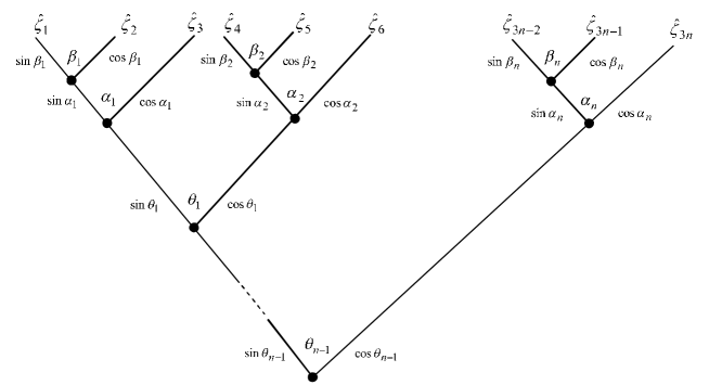
Figure 1: A tree of polyspherical coordinates for $S^{3n-1}$.

In order to write $Y_{lMK}\left(\hat{\zeta}\right)$ we make use of a graphical method called the tree method (see Section 10.5 of Ref.[30]). According to this method polyspherical coordinate systems on the sphere of unit radius can be described by graphs called trees. The trees contain nodes and each node has two edges, which are distinguished as left or right edge. An angle is associated with each node and the sine (cosine) of this angle is associated with the corresponding left (right) edge. The free (upper) ends of tree are labelled left to right with Cartesian coordinates. Then the Cartesian coordinate $\hat{\zeta}_{i}$ is equal to the product of trigonometrical functions on the edges along the unique path connecting the lowest node with  $\hat{\zeta}_{i}$. In Fig.1 we associate a tree with a polyspherical coordinate system on $S^{3n-1}$ given by formulae (21) and (32). Hence, the ($3n-1)$-dimensional spherical harmonics $Y_{lMK}\left(\hat{\zeta}\right)$ corresponding to this tree can be obtained by the rules described in Section 10.5.3 of Ref.[30]. As a result we have

$$\mathcal{Y}_{lM}\left(\hat{x}\right) = \chi\prod_{i=1}^{n-2}\sin^{m_{i}+n-i}\theta_{n-i}\cos^{\kappa_{i}+1}\theta_{n-i}P_{\left(m_{i-1}-m_{i}-\kappa_{i}\right)/2}^{\left(m_{i}+\frac{3n-3i}{2}-1,\quad\kappa_{i}+\frac{1}{2}\right)}\left(\cos 2\theta_{n-i}\right)$$ (36)

$$\times\sin^{\kappa_{n}+1}\theta_{1}\cos^{\kappa_{n-1}+1}\theta_{1}P_{\left(m_{n-2}-\kappa_{n}-\kappa_{n-1}\right)/2}^{\left(\kappa_{n}+\frac{1}{2},\quad\kappa_{n-1}+\frac{1}{2}\right)}\left(\cos 2\theta_{1}\right)\;,$$

where $P_{n}^{\left(\alpha,\beta\right)}$ are Jacobi polynomials and $\chi$ is a normalization constant

$$\chi = \prod_{i=1}^{n-2}\left[\frac{\Gamma\left(\frac{1}{2}\left(m_{i-1}+m_{i}+\kappa_{i}+3n-3i+1\right)\right)\Gamma\left(\frac{1}{2}\left(m_{i-1}-m_{i}-\kappa_{i}+2\right)\right)\left(2m_{i}+3n-3i+1\right)}{\Gamma\left(\frac{1}{2}\left(m_{i-1}+m_{i}-\kappa_{i}\right)\right)\Gamma\left(\frac{1}{2}\left(m_{i-1}-m_{i}+\kappa_{i}+3\right)\right)}\right]^{\frac{1}{2}}$$ (37)

$$\times\left[\frac{\Gamma\left(\frac{1}{2}\left(m_{n-2}+\kappa_{n}+\kappa_{n-1}+4\right)\right)\Gamma\left(\frac{1}{2}\left(m_{n-2}-\kappa_{n}-\kappa_{n-1}+2\right)\right)\left(2m_{n-2}+4\right)}{\Gamma\left(\frac{1}{2}\left(m_{n-2}+\kappa_{n}-\kappa_{n-1}+3\right)\right)\Gamma\left(\frac{1}{2}\left(m_{n-2}-\kappa_{n}+\kappa_{n-1}+3\right)\right)}\right]^{\frac{1}{2}}$$

2.2 Scattering states

Once the group structure of the problem has been recognized, the associated $S$ matrix can be computed by using matrices  that intertwine Weyl-equivalent representations of $SO\left(3n,1\right)$ in the bases corresponding to the reduction (24). We find it expedient to use, for this purpose, equation (4). By realizing the principal series of $SO\left(3n,1\right)$ on suitable Hilbert spaces of appropriate functions, one can derive from (4) the functional relations satisfied by the kernel of the intertwining operator, written in integral form and, consequently, the explicit representation of the matrix elements of the operator itself.

It is known that the most degenerate principal series representations of $SO(N,1)$ labelled with the quantum number $j=-\frac{N-1}{2}+i\rho,\$ with $\rho>0,$ can be realized on $\mathcal{L}_{2}\left(S^{N-1}\right)$ (see Section 9.2.1 of Ref[30])

$$U_{j}\left(g\right)f\left(\eta\right)=\left(\omega_{g}\right)^{j}f\left(\eta_{g}\right)\;,\quad\eta\in S^{N-1}$$ (38)

where

$$\omega_{g}=\sum_{i=1}^{N}g_{Ni}^{-1}\eta_{i}+g_{NN},\quad\left(\eta_{g}\right)_{k}=\frac{\sum_{i=1}^{N}g_{ki}^{-1}\eta_{i}+g_{kN}}{\sum_{i=1}^{N}g_{Ni}^{-1}\eta_{i}+g_{NN}}$$

The representations specified by labels $j\,\$and $1-N-j\,$ are Weyl-equivalent.

The operator $A$ defined by

$$\left(Af\right)\left(\eta\right)=\int\mathcal{K}\left(\eta,\eta^{\prime}\right)f\left(\eta^{\prime}\right)d\eta^{\prime}$$ (39)

intertwines representations $j$ and $1-N-j$ on condition that

$$\mathcal{K}\left(\eta_{g},\eta_{g}^{\prime}\right)=\left(\omega_{g}\right)^{N-1+j}\left(\omega_{g}^{\prime}\right)^{N-1+j}\mathcal{K}(\eta,\eta^{\prime})\;.$$ (40)

The kernel, $K$ , is uniquely determined by Eq. (40) up to a constant and is given by

$$\mathcal{K}(\eta,\eta^{\prime})=\varkappa\left(1-\eta\cdot\eta^{\prime}\right)^{1-N-j}\;.$$ (41)

with

$$\varkappa=2^{-\frac{N-1}{2}+{\normalsize i}\rho}\frac{\Gamma\left(\frac{N-1}{2}+{\normalsize i}\rho\right)}{\pi^{\frac{N-1}{2}}\Gamma\left(-{\normalsize i}\rho\right)}$$ (42)

Taking into account the fact that the spherical harmonics $Y_{lMK}$ (35) form a basis in $\mathcal{L}_{2}\left(S^{3n-1}\right)$, corresponding to the above reduction, we obtain the following integral representation for the matrix elements of $A$

$$\left\langle j;l^{\prime}M^{\prime}K^{\prime}\right|A\left|j;lMK\right\rangle=\int\mathcal{K}(\eta,\eta^{\prime})Y_{l^{\prime}M^{\prime}K^{\prime}}^{\ast}\left(\eta^{\prime}\right)Y_{lMK}\left(\eta\right)d\eta d\eta^{\prime}\;.$$ (43)

Therefore

$$\left\langle j;l^{\prime}M^{\prime}K^{\prime}\right|A\left|j;lMK\right\rangle=A_{l}\delta_{ll^{\prime}}\delta_{MM^{\prime}}\delta_{KK^{\prime}}\;,$$ (44)

where

$$\;A_{l}=\frac{\Gamma\left(\frac{3n-1}{2}+{\normalsize i}\rho+l\right)}{\Gamma\left(\frac{3n-1}{2}-{\normalsize i}\rho+l\right)}.$$ (45)

According to this, we have

$$S\left(p;p^{\prime}\right)=\sum\limits_{lM}A_{l}\mathcal{Y}_{lM}\left(\hat{p}\right)\mathcal{Y}_{lM}^{\ast}\left(\hat{p}^{\prime}\right)\;.$$ (46)

Thus, the scattering amplitude, $f\left(p;p^{\prime}\right)$, is defined by

$$f\left(p;p^{\prime}\right)=\left(-i\right)\left(\frac{2\pi}{p}\right)^{\frac{n-1}{2}}\sum\limits_{lM}\left(A_{l}-1\right)\mathcal{Y}_{lM}\left(\hat{p}\right)\mathcal{Y}_{lM}^{\ast}\left(\hat{p}^{\prime}\right)\;.$$ (47)

We can omit unity in the brackets of formula (47) when $\hat{p}^{\prime}\neq\hat{p}$ , leaving

$$f\left(p;p^{\prime}\right)=\left(-i\right)\left(\frac{2\pi}{p}\right)^{\frac{n-1}{2}}\sum\limits_{lM}\frac{\Gamma\left(\frac{3n-1}{2}+{\normalsize i}\rho+l\right)}{\Gamma\left(\frac{3n-1}{2}-{\normalsize i}\rho+l\right)}\mathcal{Y}_{lM}\left(\hat{p}\right)\mathcal{Y}_{lM}^{\ast}\left(\hat{p}^{\prime}\right)\;.$$ (48)

Moreover, formulae (35) and the following expansion of the kernel

$$\left(1-\eta\cdot\eta^{\prime}\right)^{-\frac{3n-1}{2}-{\normalsize i}\rho}=\left(2\pi\right)^{\frac{3n-1}{2}}\frac{2^{-i\rho}\Gamma\left(-{\normalsize i}\rho\right)}{\Gamma\left(\frac{3n-1}{2}+{\normalsize i}\rho\right)}\sum\limits_{lMK}\frac{\Gamma\left(\frac{3n-1}{2}+{\normalsize i}\rho+l\right)}{\Gamma\left(\frac{3n-1}{2}-{\normalsize i}\rho+l\right)}Y_{lMK}^{\ast}\left(\eta^{\prime}\right)Y_{lMK}\left(\eta\right)\;,$$

yield an integral representation of the scattering amplitude

$$f\left(p;p^{\prime}\right) = \frac{1}{ip^{\frac{n-1}{2}}}\frac{2^{i\rho}\Gamma\left(\frac{3n-1}{2}+{\normalsize i}\rho\right)}{\Gamma\left(-{\normalsize i}\rho\right)}\Lambda\left(\theta_{n-1},\ldots,\theta_{1}\right)\Lambda\left(\theta_{n-1}^{\prime},\ldots,\theta_{1}^{\prime}\right)$$

$$\times\int_{0}^{\pi}\cdots\int_{0}^{\pi}\left(1-\hat{p}_{1}\hat{p}_{1}^{\prime}\cos\alpha_{1}-\hat{p}_{2}\hat{p}_{2}^{\prime}\cos\alpha_{2}-\cdots-\hat{p}_{n}\hat{p}_{n}^{\prime}\cos\alpha_{n}\right)^{-\frac{3n-1}{2}-{\normalsize i}\rho}$$

$$\times P_{\kappa_{1}}\left(\cos\alpha_{1}\right)P_{\kappa_{2}}\left(\cos\alpha_{2}\right)\cdots P_{\kappa_{n}}\left(\cos\alpha_{n}\right)\sin\alpha_{1}\sin\alpha_{2}\cdots\sin\alpha_{n}d\alpha_{1}d\alpha_{2}\cdots d\alpha_{n}$$

where

$$\Lambda\left(\theta_{n-1},\ldots,\theta_{1}\right)=\prod_{i=1}^{n-1}\sin^{n-i}\theta_{n-i}\cos\theta_{n-i}$$

When $\kappa_{i}=0,$ formula (2.2) simplifies to

$$f\left(p;p^{\prime}\right)=\frac{1}{ip^{\frac{n-1}{2}}}\frac{2^{i\rho}\Gamma\left(\frac{n-1}{2}+{\normalsize i}\rho\right)}{\Gamma\left(-{\normalsize i}\rho\right)}\sum_{\epsilon_{i}=\pm}\sigma\left(1-\epsilon_{1}\hat{p}_{1}\hat{p}_{1}^{\prime}-\epsilon_{2}\hat{p}_{2}\hat{p}_{2}^{\prime}-\cdots-\epsilon_{n}\hat{p}_{n}\hat{p}_{n}^{\prime}\right)^{-\frac{n-1}{2}-{\normalsize i}\rho}$$ (50)

with

$$\sigma=\prod_{i=1}^{n}\epsilon_{i}$$

It is worth noting that the amplitude (50) does not reduce to the Coulomb amplitude $f_{Coul}$ in $n$ dimensions [4]

$$f_{Coul}\left(p;p^{\prime}\right)=\frac{1}{ip^{\frac{n-1}{2}}}\frac{2^{i\rho}\Gamma\left(\frac{n-1}{2}+{\normalsize i}\rho\right)}{\Gamma\left(-{\normalsize i}\rho\right)}\left(1-\hat{p}_{1}\hat{p}_{1}^{\prime}-\hat{p}_{2}\hat{p}_{2}^{\prime}-\cdots-\hat{p}_{n}\hat{p}_{n}^{\prime}\right)^{-\frac{n-1}{2}-{\normalsize i}\rho}$$ (51)

when $\kappa_{i}$ is set equal to zero. The reason for this discrepancy lies in the fact that we solve the Schrödinger equation for $x_{i}\geq 0,\ (i=1,2,\ldots,n)$  with boundary conditions

$$\Psi\left(x\right)=0\textstyle{\ \ for\ \ }x_{i}=0,\;(i=1,\ldots,n)$$

3 Conclusions and outlook

The present work is the latest in a series of papers where the potential group approach and the method of intertwining operators (formulae (2-7)) have been applied to non-central extensions of the Coulomb potential: Ref.[31] studied the bound states of the three-dimensional Coulomb potential plus a barrier term with the $SO\left(5\right)$ potential group and Ref.[32] the scattering states of similar potentials with $SO\left(5,1\right)$ potential group. A first simultaneous analysis of bound and scattering states of a three-dimensional Coulomb-Rosochatius potential of type (8) was performed in Ref[33], where the use of potential groups $SO\left(7\right)$ for bound states and $SO\left(6,1\right)$ for scattering states. Generally, in the $n$-dimensional case for Coulomb-Rosochatius potential one can choose potential groups $SO\left(qn+1\right)$ and $SO\left(qn,1\right)$ with $q=2,3,\ldots$ . Then the potential strengths $\beta_{i}$ will be related to eigenvalues $k_{i}\left(k_{i}+q-2\right),\ k_{i}=0,1,2,\ldots,$ of Casimir operators of subgroups $SO\left(q\right)_{i}$ as: $\beta_{i}=\left(k_{i}+\frac{q-2}{2}\right)^{2}-\frac{1}{4}.$ In the present work, we have chosen $q=3$.

The method has proved useful also in deriving the full set of  $2n-1$ constants of motion, related to Casimir invariants of subgroups appearing in the decomposition chains, thus proving the maximal superintegrability of the system.

The potential group approach is quite general and, obviously, not limited to the orthogonal and pseudo-orthogonal symmetries underlying the Coulomb-Rosochatius Hamiltonian. Systems with different symmetries will be studied in future works.

References

• [1] Alliluev SP 1958 Sov. Phys.-JETP 6 156.
• [2] Bander M and Itzykson C 1966 Rev. Mod. Phys. 38 330.
• [3] Bander M and Itzykson C 1966 Rev. Mod. Phys.38 346.
• [4] Rasmussen WO and SalamΓ³ S 1979 J. Math. Phys. 20 1064.
• [5] Nieto MM 1979 Am. J. Phys. 47 1067.
• [6] Kostelecky VA and Nieto MM 1985 Phys. Rev. D 32 2627.
• [7] Thieleker E 1989 Pacific J. Math. 139 339.
• [8] Zeng GJ, Su KL and Li M 1994 Phys. Rev. A 50 4373.
• [9] Kostelecky VA and Russell N 1996 J. Math. Phys. 37 2166.
• [10] Yafaev D 1997 J. Phys. A: Math. Gen 30 6981.
• [11] Daboul C and Daboul J 1998 Phys.Lett.B 425 135.
• [12] LΓ©vai G, Konya B and Papp Z 1998 J. Math. Phys. 39 5811.
• [13] Nouri S 1999 J. Math. Phys. 40 1294.
• [14] Fock VA 1935 Z. Phys.98 145.
• [15] Bargmann V 1936 Z. Phys. 99 576.
• [16] Barut AO 1972 Dynamical and Generalized Symmetries in Quantum Theory (University of Canterbury Press, Christchurch, New Zealand).
• [17] Tempesta P, Winternitz P, Harnad J, Miller Jr JW, G. Pogosyan RodrΓ­guez MA, eds.,2004 Β Superintegrability in Classical and Quantum Systems, MontrΓ©al, CRM Proceedings and Lecture Notes 37, American Mathematical Society.
• [18] Rosochatius E 1877 Ε°ber die Bewegung eines Punktes , inaugural dissertation, University of GΕ‘ttingen (Unger, Berlin).
• [19] Verrier PE and Evans NW 2008, J. Math. Phys.Β 49 022902.
• [20] RodrΓ­guez MA, Tempesta P and Winternitz P 2009 J. Phys. Conf. Ser. 175 012013.
• [21] Makarov AA, Smorodinsky JA, Valiev Kh and Winternitz P 1967 Nuovo Cimento 52 A 1061.
• [22] Evans NW 1990 Phys. Rev. A Β 41 5666.
• [23] Ballestreros Á and Herranz FJ 2009 J. Phys. A: Math. Theor.42 245203.
• [24] Alhassid Y, GΓΌrsey F and Iachello F 1983, Ann. Phys. Β 148 346.
• [25] Ghirardi GC 1972 Nuovo Cimento A 10 97.
• [26] Scarf FL 1958 Phys. Rev. 112 1137.
• [27] Olshanetsky MA and Perelomov AM 1977 Lett. Math. Phys.Β 2 7.
• [28] Olshanetsky MA and Perelomov AM 1983 Phys. Rep.94 313.
• [29] Kerimov GA 1998 Phys. Rev. Lett.80 2976.
• [30] Vilenkin NJa and Klimyk AU 1993 Representation of Lie Goups and Special Functions , Vol. 2 (Kluwer Academic Publishers, Dordrecht, Holland).
• [31] Kerimov GA 2006 J. Phys. A: Math. Gen.39 1183.
• [32] Kerimov GA 2007 J. Phys. A: Math. Theor. 40 7297.
• [33] Kerimov GA and Ventura A 2010 J. Phys. A: Math. Theor. 43 255304.