1 Introduction
Motions on hyperbolic spaces have been studied since the end of the Fifties and most of the papers devoted to them deal with the so-called hyperbolic Brownian motion (see, e.g., Gertsenshtein and Vasiliev [4 ] , Gruet [5 ] , Monthus and Texier [9 ] , Lao and Orsingher [7 ] ).
More recently also works concerning two-dimensional random motions at finite velocity on planar hyperbolic spaces have been introduced and analyzed (Orsingher and De Gregorio [11 ] ).
While in [11 ] the components of motion are supposed to be independent, we present here a planar random motion with interacting components. Its counterpart on the unit sphere is also examined and discussed.
The space on which our motion develops is the Poincaré upper half-plane H 2 + = { ( x , y ) : y > 0 } superscript subscript 𝐻 2 conditional-set 𝑥 𝑦 𝑦 0 H_{2}^{+}=\{(x,y):y>0\} H 2 + subscript superscript 𝐻 2 H^{+}_{2}
d s 2 = d x 2 + d y 2 y 2 . d superscript 𝑠 2 d superscript 𝑥 2 d superscript 𝑦 2 superscript 𝑦 2 \mathrm{d}s^{2}=\frac{\mathrm{d}x^{2}+\mathrm{d}y^{2}}{y^{2}}. (1.1)
The propagation of light in a planar non-homogeneous medium, according to the Fermat principle, must obey the law
sin α ( y ) c ( x , y ) = cost 𝛼 𝑦 𝑐 𝑥 𝑦 cost \frac{\sin\alpha(y)}{c(x,y)}=\mathrm{cost} (1.2)
where α ( y ) 𝛼 𝑦 \alpha(y) y 𝑦 y c ( x , y ) = y 𝑐 𝑥 𝑦 𝑦 c(x,y)=y H 2 + superscript subscript 𝐻 2 H_{2}^{+}
In [2 ] it is shown that the light propagates in a non-homogeneous half-plane H 2 + superscript subscript 𝐻 2 H_{2}^{+} n ( x , y ) = 1 / y 𝑛 𝑥 𝑦 1 𝑦 n(x,y)=1/y
Scattered obstacles in the non-homogeneous medium cause random deviations in the propagation of light and this leads to the random model analyzed below.
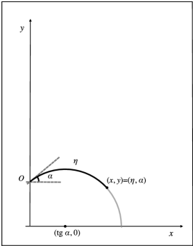
The position of points in H 2 + superscript subscript 𝐻 2 H_{2}^{+} ( x , y ) 𝑥 𝑦 (x,y) ( η , α ) 𝜂 𝛼 (\eta,\alpha) η 𝜂 \eta H 2 + superscript subscript 𝐻 2 H_{2}^{+} O 𝑂 O ( 0 , 1 ) 0 1 (0,1) η 𝜂 \eta 1.1 x 𝑥 x ( x , y ) 𝑥 𝑦 (x,y) O 𝑂 O x 𝑥 x H 2 + superscript subscript 𝐻 2 H_{2}^{+}
The angle α 𝛼 \alpha O 𝑂 O ( x , y ) 𝑥 𝑦 (x,y) 1
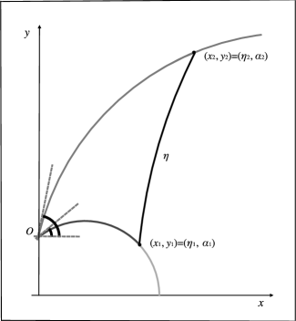
Figure 1: Figure 1(a) illustrates the hyperbolic coordinates. Figure 1(b) refers to the hyperbolic triangle of Carnot formula.
The formulas which relate the polar hyperbolic coordinates ( η , α ) 𝜂 𝛼 (\eta,\alpha) ( x , y ) 𝑥 𝑦 (x,y) [12 ] , page 213)
{ x = sinh η cos α cosh η − sinh η sin α η > 0 , y = 1 cosh η − sinh η sin α − π 2 < α < π 2 . cases 𝑥 𝜂 𝛼 𝜂 𝜂 𝛼 𝜂 0 𝑦 1 𝜂 𝜂 𝛼 𝜋 2 𝛼 𝜋 2 \left\{\begin{array}[]{lr}x=\frac{\sinh\eta\cos\alpha}{\cosh\eta-\sinh\eta\sin\alpha}&\eta>0,\\
y=\frac{1}{\cosh\eta-\sinh\eta\sin\alpha}&-\frac{\pi}{2}<\alpha<\frac{\pi}{2}.\end{array}\right. (1.3)
For each value of α 𝛼 \alpha
( x − tan α ) 2 + y 2 = 1 cos 2 α . superscript 𝑥 𝛼 2 superscript 𝑦 2 1 superscript 2 𝛼 (x-\tan\alpha)^{2}+y^{2}=\frac{1}{\cos^{2}\alpha}. (1.4)
For α = π 2 𝛼 𝜋 2 \alpha=\frac{\pi}{2} 1.4 y 𝑦 y H 2 + superscript subscript 𝐻 2 H_{2}^{+}
From (1.3 η 𝜂 \eta ( x , y ) 𝑥 𝑦 (x,y) O 𝑂 O
cosh η = x 2 + y 2 + 1 2 y . 𝜂 superscript 𝑥 2 superscript 𝑦 2 1 2 𝑦 \cosh\eta=\frac{x^{2}+y^{2}+1}{2y}. (1.5)
From (1.5 η 𝜂 \eta O 𝑂 O ( 0 , cosh η ) 0 𝜂 (0,\cosh\eta) sinh η 𝜂 \sinh\eta
The expression of the hyperbolic distance between two arbitrary points ( x 1 , y 1 ) subscript 𝑥 1 subscript 𝑦 1 (x_{1},y_{1}) ( x 2 , y 2 ) subscript 𝑥 2 subscript 𝑦 2 (x_{2},y_{2})
cosh η = ( x 1 − x 2 ) 2 + y 1 2 + y 2 2 2 y 1 y 2 . 𝜂 superscript subscript 𝑥 1 subscript 𝑥 2 2 superscript subscript 𝑦 1 2 superscript subscript 𝑦 2 2 2 subscript 𝑦 1 subscript 𝑦 2 \cosh\eta=\frac{(x_{1}-x_{2})^{2}+y_{1}^{2}+y_{2}^{2}}{2y_{1}y_{2}}. (1.6)
In fact, by considering the hyperbolic triangle with vertices at ( 0 , 1 ) 0 1 (0,1) ( x 1 , y 1 ) subscript 𝑥 1 subscript 𝑦 1 (x_{1},y_{1}) ( x 2 , y 2 ) subscript 𝑥 2 subscript 𝑦 2 (x_{2},y_{2}) η 𝜂 \eta ( x 1 , y 1 ) subscript 𝑥 1 subscript 𝑦 1 (x_{1},y_{1}) ( x 2 , y 2 ) subscript 𝑥 2 subscript 𝑦 2 (x_{2},y_{2})
cosh η = cosh η 1 cosh η 2 − sinh η 1 sinh η 2 cos ( α 1 − α 2 ) 𝜂 subscript 𝜂 1 subscript 𝜂 2 subscript 𝜂 1 subscript 𝜂 2 subscript 𝛼 1 subscript 𝛼 2 \cosh\eta=\cosh\eta_{1}\cosh\eta_{2}-\sinh\eta_{1}\sinh\eta_{2}\cos(\alpha_{1}-\alpha_{2}) (1.7)
where ( η 1 , α 1 ) subscript 𝜂 1 subscript 𝛼 1 (\eta_{1},\alpha_{1}) ( η 2 , α 2 ) subscript 𝜂 2 subscript 𝛼 2 (\eta_{2},\alpha_{2}) ( x 1 , y 1 ) subscript 𝑥 1 subscript 𝑦 1 (x_{1},y_{1}) ( x 2 , y 2 ) subscript 𝑥 2 subscript 𝑦 2 (x_{2},y_{2}) 1 1.4
tan α i = x i 2 + y i 2 − 1 2 x i for i = 1 , 2 , formulae-sequence subscript 𝛼 𝑖 superscript subscript 𝑥 𝑖 2 superscript subscript 𝑦 𝑖 2 1 2 subscript 𝑥 𝑖 for 𝑖 1 2
\tan\alpha_{i}=\frac{x_{i}^{2}+y_{i}^{2}-1}{2x_{i}}\mathrm{\;\;\;\;\;\;for\;}i=1,2, (1.8)
and view of (1.5 1.8 1.6 ( x 1 , y 1 ) subscript 𝑥 1 subscript 𝑦 1 (x_{1},y_{1}) ( 0 , 1 ) 0 1 (0,1)
If α 1 − α 2 = π 2 subscript 𝛼 1 subscript 𝛼 2 𝜋 2 \alpha_{1}-\alpha_{2}=\frac{\pi}{2} 1.7
cosh η = cosh η 1 cosh η 2 𝜂 subscript 𝜂 1 subscript 𝜂 2 \cosh\eta=\cosh\eta_{1}\cosh\eta_{2} (1.9)
which plays an important role in the present paper.
The motion considered here is the non-Euclidean counterpart of the planar motion with orthogonal deviations studied in Orsingher [10 ] . The main object of the investigation is the hyperbolic distance of the moving point from the origin. We are able to give explicit expressions for its mean value, also under the condition that the number of changes of direction is known. In the case of motion in H 2 + superscript subscript 𝐻 2 H_{2}^{+} [11 ] ) an explicit expression for the distribution of the hyperbolic distance η 𝜂 \eta η ( t ) 𝜂 𝑡 \eta(t)
We obtain the following explicit formula for the mean value of the hyperbolic distance which reads
E { cosh η ( t ) } 𝐸 𝜂 𝑡 \displaystyle E\{\cosh\eta(t)\} = \displaystyle= e − λ t 2 { cosh t 2 λ 2 + 4 c 2 + λ λ 2 + 4 c 2 sinh t 2 λ 2 + 4 c 2 } superscript 𝑒 𝜆 𝑡 2 𝑡 2 superscript 𝜆 2 4 superscript 𝑐 2 𝜆 superscript 𝜆 2 4 superscript 𝑐 2 𝑡 2 superscript 𝜆 2 4 superscript 𝑐 2 \displaystyle e^{-\frac{\lambda t}{2}}\left\{\cosh\frac{t}{2}\sqrt{\lambda^{2}+4c^{2}}+\frac{\lambda}{\sqrt{\lambda^{2}+4c^{2}}}\sinh\frac{t}{2}\sqrt{\lambda^{2}+4c^{2}}\right\} (1.10)
= \displaystyle= E e T ( t ) 𝐸 superscript 𝑒 𝑇 𝑡 \displaystyle Ee^{T(t)}
where T ( t ) 𝑇 𝑡 T(t) λ 2 𝜆 2 \frac{\lambda}{2} 2 c 2 𝑐 2c
The telegraph process represents the random motion of a particle moving with constant velocity and changing direction at Poisson-paced times (see, for example [11 ] ).
Section 5 5 5 T 1 subscript 𝑇 1 T_{1} η 1 ( t ) subscript 𝜂 1 𝑡 \eta_{1}(t)
E { cosh η 1 ( t ) | N ( t ) ≥ 1 } = λ λ 2 + 4 c 2 sinh t 2 λ 2 + 4 c 2 sinh λ t 2 . 𝐸 conditional-set subscript 𝜂 1 𝑡 𝑁 𝑡 1 𝜆 superscript 𝜆 2 4 superscript 𝑐 2 𝑡 2 superscript 𝜆 2 4 superscript 𝑐 2 𝜆 𝑡 2 E\{\cosh\eta_{1}(t)|N(t)\geq 1\}=\frac{\lambda}{\sqrt{\lambda^{2}+4c^{2}}}\frac{\sinh\frac{t}{2}\sqrt{\lambda^{2}+4c^{2}}}{\sinh\frac{\lambda t}{2}}. (1.11)
The last section considers the motion at finite velocity, with
orthogonal deviations at Poisson times, on the unit-radius sphere.
The main results concern the mean value E { cos d ( P 0 P t ) } 𝐸 d subscript 𝑃 0 subscript 𝑃 𝑡 E\{\cos\mathrm{d}(P_{0}P_{t})\} d ( P 0 P t ) d subscript 𝑃 0 subscript 𝑃 𝑡 \mathrm{d}(P_{0}P_{t}) P t subscript 𝑃 𝑡 P_{t} P 0 subscript 𝑃 0 P_{0}
2 Description of the Planar Random Motion on the Poincaré Half-Plane H 2 + superscript subscript 𝐻 2 H_{2}^{+}
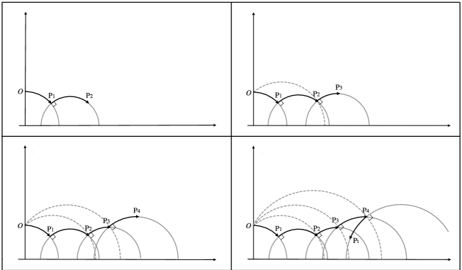
We start our analysis by considering a particle located at the origin O 𝑂 O H 2 + superscript subscript 𝐻 2 H_{2}^{+} ( 0 , 0 ) 0 0 (0,0) 1 1 1 x 𝑥 x λ 𝜆 \lambda
At the occurrence of the first Poisson event, the particle starts moving on the circumference orthogonal to the previous one.
After having reached the point P 2 subscript 𝑃 2 P_{2} O 𝑂 O P 2 subscript 𝑃 2 P_{2} 2
In general, at the n 𝑛 n P n subscript 𝑃 𝑛 P_{n} P n subscript 𝑃 𝑛 P_{n} O 𝑂 O 2
At each Poisson event the particle moves from the reached position P 𝑃 P 1 2 1 2 \frac{1}{2} P 𝑃 P O 𝑂 O
Figure 2: In the first three figures a sample path where the particle chooses the outward direction is depicted. In the last one a trajectory with one step moving towards the origin is depicted.
The hyperbolic length of the arc run by the particle during the inter-time between two successive changes of direction, occurring at t k − 1 subscript 𝑡 𝑘 1 t_{k-1} t k subscript 𝑡 𝑘 t_{k} c ( t k − t k − 1 ) 𝑐 subscript 𝑡 𝑘 subscript 𝑡 𝑘 1 c(t_{k}-t_{k-1}) k ≥ 1 𝑘 1 k\geq 1 t 0 = 0 subscript 𝑡 0 0 t_{0}=0 c 𝑐 c
c = d s d t = 1 y d x 2 + d y 2 d t 2 . 𝑐 d 𝑠 d 𝑡 1 𝑦 d superscript 𝑥 2 d superscript 𝑦 2 d superscript 𝑡 2 c=\frac{\mathrm{d}s}{\mathrm{d}t}=\frac{1}{y}\sqrt{\frac{\mathrm{d}x^{2}+\mathrm{d}y^{2}}{\mathrm{d}t^{2}}}. (2.1)
The Cartesian coordinates of the points P k subscript 𝑃 𝑘 P_{k}
The construction outlined above shows that the arcs O P k − 1 𝑂 subscript 𝑃 𝑘 1 OP_{k-1} P k − 1 P k subscript 𝑃 𝑘 1 subscript 𝑃 𝑘 P_{k-1}P_{k} O P k 𝑂 subscript 𝑃 𝑘 OP_{k} P k − 1 subscript 𝑃 𝑘 1 P_{k-1}
cosh d ( O P k ) = cosh d ( O P k − 1 ) cosh d ( P k − 1 P k ) . d 𝑂 subscript 𝑃 𝑘 d 𝑂 subscript 𝑃 𝑘 1 d subscript 𝑃 𝑘 1 subscript 𝑃 𝑘 \cosh\mathrm{d}(OP_{k})=\cosh\mathrm{d}(OP_{k-1})\cosh\mathrm{d}(P_{k-1}P_{k}). (2.2)
The hyperbolic distance η ( t ) 𝜂 𝑡 \eta(t) P t subscript 𝑃 𝑡 P_{t} n 𝑛 n
cosh η ( t ) 𝜂 𝑡 \displaystyle\cosh\eta(t) = \displaystyle= cosh d ( O P t ) d 𝑂 subscript 𝑃 𝑡 \displaystyle\cosh\mathrm{d}(OP_{t}) (2.3)
= \displaystyle= cosh d ( P n P t ) cosh d ( O P n ) d subscript 𝑃 𝑛 subscript 𝑃 𝑡 d 𝑂 subscript 𝑃 𝑛 \displaystyle\cosh\mathrm{d}(P_{n}P_{t})\cosh\mathrm{d}(OP_{n})
= \displaystyle= cosh c ( t − t n ) ∏ k = 1 n cosh c ( t k − t k − 1 ) 𝑐 𝑡 subscript 𝑡 𝑛 superscript subscript product 𝑘 1 𝑛 𝑐 subscript 𝑡 𝑘 subscript 𝑡 𝑘 1 \displaystyle\cosh c(t-t_{n})\prod_{k=1}^{n}\cosh c(t_{k}-t_{k-1})
= \displaystyle= ∏ k = 1 n + 1 cosh c ( t k − t k − 1 ) , superscript subscript product 𝑘 1 𝑛 1 𝑐 subscript 𝑡 𝑘 subscript 𝑡 𝑘 1 \displaystyle\prod_{k=1}^{n+1}\cosh c(t_{k}-t_{k-1}),
where t 0 = 0 subscript 𝑡 0 0 t_{0}=0 t n + 1 = t subscript 𝑡 𝑛 1 𝑡 t_{n+1}=t t k subscript 𝑡 𝑘 t_{k} k = 0 , 1 , … , n 𝑘 0 1 … 𝑛
k=0,1,\dots,n
T = { 0 = t 0 < t 1 < ⋯ < t k < ⋯ < t n < t n + 1 = t } . 𝑇 0 subscript 𝑡 0 subscript 𝑡 1 ⋯ subscript 𝑡 𝑘 ⋯ subscript 𝑡 𝑛 subscript 𝑡 𝑛 1 𝑡 T=\{0=t_{0}<t_{1}<\cdots<t_{k}<\cdots<t_{n}<t_{n+1}=t\}. (2.4)
This means that cosh η ( t ) 𝜂 𝑡 \cosh\eta(t) 2.3 O 𝑂 O N ( t ) = n 𝑁 𝑡 𝑛 N(t)=n
We remark that the geodesic distance (2.3 2.3 n 𝑛 n c 𝑐 c
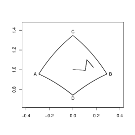
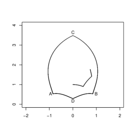
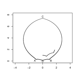
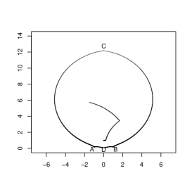
Figure 3: The set of all possible points reachable by the process for different values of t 𝑡 t c = 0.05 𝑐 0.05 c=0.05 N ( t ) = 2 𝑁 𝑡 2 N(t)=2
The set of possible positions at different times t 𝑡 t 3 A 𝐴 A B 𝐵 B C 𝐶 C D 𝐷 D
The ensemble of points having the same hyperbolic distance from O 𝑂 O t 𝑡 t C = ( 0 , cosh η ( t ) ) 𝐶 0 𝜂 𝑡 C=(0,\cosh\eta(t)) sinh η ( t ) 𝜂 𝑡 \sinh\eta(t)
cosh η ( t ) = ∏ k = 1 n + 1 cosh c ( t k − t k − 1 ) , 𝜂 𝑡 superscript subscript product 𝑘 1 𝑛 1 𝑐 subscript 𝑡 𝑘 subscript 𝑡 𝑘 1 \cosh\eta(t)=\prod_{k=1}^{n+1}\cosh c(t_{k}-t_{k-1}), (2.5)
the ordinate of the center C 𝐶 C
∏ k = 1 n + 1 sinh c ( t k − t k − 1 ) superscript subscript product 𝑘 1 𝑛 1 𝑐 subscript 𝑡 𝑘 subscript 𝑡 𝑘 1 \prod_{k=1}^{n+1}\sinh c(t_{k}-t_{k-1}) (2.6)
because
sinh η ( t ) ≥ ∏ k = 1 n + 1 sinh c ( t k − t k − 1 ) 𝜂 𝑡 superscript subscript product 𝑘 1 𝑛 1 𝑐 subscript 𝑡 𝑘 subscript 𝑡 𝑘 1 \sinh\eta(t)\geq\prod_{k=1}^{n+1}\sinh c(t_{k}-t_{k-1}) (2.7)
and (2.6 t 𝑡 t
3 The Equations Related to the Mean Hyperbolic Distance
In this section we study the conditional and unconditional mean values of the hyperbolic distance η ( t ) 𝜂 𝑡 \eta(t)
E n ( t ) subscript 𝐸 𝑛 𝑡 \displaystyle E_{n}(t) = \displaystyle= E { cosh η ( t ) | N ( t ) = n } 𝐸 conditional-set 𝜂 𝑡 𝑁 𝑡 𝑛 \displaystyle E\{\cosh\eta(t)|N(t)=n\}
= \displaystyle= n ! t n ∫ 0 t d t 1 ∫ t 1 t d t 2 ⋯ ∫ t n − 1 t d t n ∏ k = 1 n + 1 cosh c ( t k − t k − 1 ) 𝑛 superscript 𝑡 𝑛 superscript subscript 0 𝑡 differential-d subscript 𝑡 1 superscript subscript subscript 𝑡 1 𝑡 differential-d subscript 𝑡 2 ⋯ superscript subscript subscript 𝑡 𝑛 1 𝑡 differential-d subscript 𝑡 𝑛 superscript subscript product 𝑘 1 𝑛 1 𝑐 subscript 𝑡 𝑘 subscript 𝑡 𝑘 1 \displaystyle\frac{n!}{t^{n}}\int_{0}^{t}\mathrm{d}t_{1}\int_{t_{1}}^{t}\mathrm{d}t_{2}\cdots\int_{t_{n-1}}^{t}\mathrm{d}t_{n}\prod_{k=1}^{n+1}\cosh c(t_{k}-t_{k-1})
= \displaystyle= n ! t n I n ( t ) , 𝑛 superscript 𝑡 𝑛 subscript 𝐼 𝑛 𝑡 \displaystyle\frac{n!}{t^{n}}I_{n}(t),
where
I n ( t ) = ∫ 0 t d t 1 ⋯ ∫ t n − 1 t d t n ∏ k = 1 n + 1 cosh c ( t k − t k − 1 ) , subscript 𝐼 𝑛 𝑡 superscript subscript 0 𝑡 differential-d subscript 𝑡 1 ⋯ superscript subscript subscript 𝑡 𝑛 1 𝑡 differential-d subscript 𝑡 𝑛 superscript subscript product 𝑘 1 𝑛 1 𝑐 subscript 𝑡 𝑘 subscript 𝑡 𝑘 1 I_{n}(t)=\int_{0}^{t}\mathrm{d}t_{1}\cdots\int_{t_{n-1}}^{t}\mathrm{d}t_{n}\prod_{k=1}^{n+1}\cosh c(t_{k}-t_{k-1}), (3.2)
and by
E ( t ) 𝐸 𝑡 \displaystyle E(t) = \displaystyle= E { cosh η ( t ) } 𝐸 𝜂 𝑡 \displaystyle E\{\cosh\eta(t)\}
= \displaystyle= ∑ n = 0 ∞ E { cosh η ( t ) | N ( t ) = n } P r { N ( t ) = n } superscript subscript 𝑛 0 𝐸 conditional-set 𝜂 𝑡 𝑁 𝑡 𝑛 𝑃 𝑟 𝑁 𝑡 𝑛 \displaystyle\sum_{n=0}^{\infty}E\{\cosh\eta(t)|N(t)=n\}Pr\{N(t)=n\}
= \displaystyle= e − λ t ∑ n = 0 ∞ λ n I n ( t ) . superscript 𝑒 𝜆 𝑡 superscript subscript 𝑛 0 superscript 𝜆 𝑛 subscript 𝐼 𝑛 𝑡 \displaystyle e^{-\lambda t}\sum_{n=0}^{\infty}\lambda^{n}I_{n}(t).
At first, we state the following result concerning the evaluation of the integrals I n ( t ) subscript 𝐼 𝑛 𝑡 I_{n}(t) n ≥ 1 𝑛 1 n\geq 1
Lemma 3.1 .
The functions
I n ( t ) = ∫ 0 t d t 1 ∫ t 1 t d t 2 ⋯ ∫ t n − 1 t d t n ∏ k = 1 n + 1 cosh c ( t k − t k − 1 ) , subscript 𝐼 𝑛 𝑡 superscript subscript 0 𝑡 differential-d subscript 𝑡 1 superscript subscript subscript 𝑡 1 𝑡 differential-d subscript 𝑡 2 ⋯ superscript subscript subscript 𝑡 𝑛 1 𝑡 differential-d subscript 𝑡 𝑛 superscript subscript product 𝑘 1 𝑛 1 𝑐 subscript 𝑡 𝑘 subscript 𝑡 𝑘 1 I_{n}(t)=\int_{0}^{t}\mathrm{d}t_{1}\int_{t_{1}}^{t}\mathrm{d}t_{2}\cdots\int_{t_{n-1}}^{t}\mathrm{d}t_{n}\prod_{k=1}^{n+1}\cosh c(t_{k}-t_{k-1}), (3.4)
with t 0 = 0 subscript 𝑡 0 0 t_{0}=0 t n + 1 = t subscript 𝑡 𝑛 1 𝑡 t_{n+1}=t
d 2 d t 2 I n = d d t I n − 1 + c 2 I n superscript d 2 d superscript 𝑡 2 subscript 𝐼 𝑛 d d 𝑡 subscript 𝐼 𝑛 1 superscript 𝑐 2 subscript 𝐼 𝑛 \frac{\mathrm{d}^{2}}{\mathrm{d}t^{2}}I_{n}=\frac{\mathrm{d}}{\mathrm{d}t}I_{n-1}+c^{2}I_{n} (3.5)
where t > 0 𝑡 0 t>0 n ≥ 1 𝑛 1 n\geq 1 I 0 ( t ) = cosh c t subscript 𝐼 0 𝑡 𝑐 𝑡 I_{0}(t)=\cosh{ct}
Proof
We first note that
d d t I n d d 𝑡 subscript 𝐼 𝑛 \displaystyle\frac{\mathrm{d}}{\mathrm{d}t}I_{n} = \displaystyle= ∫ 0 t d t 1 ⋯ ∫ t n − 2 t d t n − 1 ∏ k = 1 n cosh c ( t k − t k − 1 ) superscript subscript 0 𝑡 differential-d subscript 𝑡 1 ⋯ superscript subscript subscript 𝑡 𝑛 2 𝑡 differential-d subscript 𝑡 𝑛 1 superscript subscript product 𝑘 1 𝑛 𝑐 subscript 𝑡 𝑘 subscript 𝑡 𝑘 1 \displaystyle\int_{0}^{t}\mathrm{d}t_{1}\cdots\int_{t_{n-2}}^{t}\mathrm{d}t_{n-1}\prod_{k=1}^{n}\cosh c(t_{k}-t_{k-1})
+ \displaystyle+ c ∫ 0 t d t 1 ⋯ ∫ t n − 1 t d t n ∏ k = 1 n cosh c ( t k − t k − 1 ) sinh c ( t − t n ) 𝑐 superscript subscript 0 𝑡 differential-d subscript 𝑡 1 ⋯ superscript subscript subscript 𝑡 𝑛 1 𝑡 differential-d subscript 𝑡 𝑛 superscript subscript product 𝑘 1 𝑛 𝑐 subscript 𝑡 𝑘 subscript 𝑡 𝑘 1 𝑐 𝑡 subscript 𝑡 𝑛 \displaystyle c\int_{0}^{t}\mathrm{d}t_{1}\cdots\int_{t_{n-1}}^{t}\mathrm{d}t_{n}\prod_{k=1}^{n}\cosh c(t_{k}-t_{k-1})\sinh c(t-t_{n})
= \displaystyle= I n − 1 + c ∫ 0 t d t 1 ⋯ ∫ t n − 1 t d t n ∏ k = 1 n cosh c ( t k − t k − 1 ) sinh c ( t − t n ) subscript 𝐼 𝑛 1 𝑐 superscript subscript 0 𝑡 differential-d subscript 𝑡 1 ⋯ superscript subscript subscript 𝑡 𝑛 1 𝑡 differential-d subscript 𝑡 𝑛 superscript subscript product 𝑘 1 𝑛 𝑐 subscript 𝑡 𝑘 subscript 𝑡 𝑘 1 𝑐 𝑡 subscript 𝑡 𝑛 \displaystyle I_{n-1}+c\int_{0}^{t}\mathrm{d}t_{1}\cdots\int_{t_{n-1}}^{t}\mathrm{d}t_{n}\prod_{k=1}^{n}\cosh c(t_{k}-t_{k-1})\sinh c(t-t_{n})
and therefore
d 2 d t 2 I n superscript d 2 d superscript 𝑡 2 subscript 𝐼 𝑛 \displaystyle\frac{\mathrm{d}^{2}}{\mathrm{d}t^{2}}I_{n} = \displaystyle= d d t I n − 1 + c 2 ∫ 0 t d t 1 ⋯ ∫ t n − 1 t d t n ∏ k = 1 n + 1 cosh c ( t k − t k − 1 ) d d 𝑡 subscript 𝐼 𝑛 1 superscript 𝑐 2 superscript subscript 0 𝑡 differential-d subscript 𝑡 1 ⋯ superscript subscript subscript 𝑡 𝑛 1 𝑡 differential-d subscript 𝑡 𝑛 superscript subscript product 𝑘 1 𝑛 1 𝑐 subscript 𝑡 𝑘 subscript 𝑡 𝑘 1 \displaystyle\frac{\mathrm{d}}{\mathrm{d}t}I_{n-1}+c^{2}\int_{0}^{t}\mathrm{d}t_{1}\cdots\int_{t_{n-1}}^{t}\mathrm{d}t_{n}\prod_{k=1}^{n+1}\cosh c(t_{k}-t_{k-1}) (3.7)
= \displaystyle= d d t I n − 1 + c 2 I n . d d 𝑡 subscript 𝐼 𝑛 1 superscript 𝑐 2 subscript 𝐼 𝑛 \displaystyle\frac{\mathrm{d}}{\mathrm{d}t}I_{n-1}+c^{2}I_{n}.
■ ■ \blacksquare
In view of Lemma 3.1
Theorem 3.2 .
The mean value E ( t ) = E { cosh η ( t ) } 𝐸 𝑡 𝐸 𝜂 𝑡 E(t)=E\{\cosh\eta(t)\}
d 2 d t 2 E ( t ) = − λ d d t E ( t ) + c 2 E ( t ) superscript d 2 d superscript 𝑡 2 𝐸 𝑡 𝜆 d d 𝑡 𝐸 𝑡 superscript 𝑐 2 𝐸 𝑡 \frac{\mathrm{d}^{2}}{\mathrm{d}t^{2}}E(t)=-\lambda\frac{\mathrm{d}}{\mathrm{d}t}E(t)+c^{2}E(t) (3.8)
with initial conditions
{ E ( 0 ) = 1 , d d t E ( t ) | t = 0 = 0 . cases 𝐸 0 1 missing-subexpression evaluated-at d d 𝑡 𝐸 𝑡 𝑡 0 0 missing-subexpression \left\{\begin{array}[]{lr}E(0)=1,\\
\left.\frac{\mathrm{d}}{\mathrm{d}t}E(t)\right|_{t=0}=0.\end{array}\right. (3.9)
The explicit value of the mean hyperbolic distance is therefore
E ( t ) = e − λ t 2 { cosh t λ 2 + 4 c 2 2 + λ λ 2 + 4 c 2 sinh t λ 2 + 4 c 2 2 } . 𝐸 𝑡 superscript 𝑒 𝜆 𝑡 2 𝑡 superscript 𝜆 2 4 superscript 𝑐 2 2 𝜆 superscript 𝜆 2 4 superscript 𝑐 2 𝑡 superscript 𝜆 2 4 superscript 𝑐 2 2 E(t)=e^{-\frac{\lambda t}{2}}\left\{\cosh\frac{t\sqrt{\lambda^{2}+4c^{2}}}{2}+\frac{\lambda}{\sqrt{\lambda^{2}+4c^{2}}}\sinh\frac{t\sqrt{\lambda^{2}+4c^{2}}}{2}\right\}. (3.10)
Proof
From (3
d d t E ( t ) = − λ E ( t ) + e − λ t ∑ n = 0 ∞ λ n d d t I n d d 𝑡 𝐸 𝑡 𝜆 𝐸 𝑡 superscript 𝑒 𝜆 𝑡 superscript subscript 𝑛 0 superscript 𝜆 𝑛 d d 𝑡 subscript 𝐼 𝑛 \frac{\mathrm{d}}{\mathrm{d}t}E(t)=-\lambda E(t)+e^{-\lambda t}\sum_{n=0}^{\infty}\lambda^{n}\frac{\mathrm{d}}{\mathrm{d}t}I_{n} (3.11)
and thus, in view of (3.7 I − 1 = 0 subscript 𝐼 1 0 I_{-1}=0
d 2 d t 2 E ( t ) superscript d 2 d superscript 𝑡 2 𝐸 𝑡 \displaystyle\frac{\mathrm{d}^{2}}{\mathrm{d}t^{2}}E(t)
= − λ d d t E ( t ) − λ ( d d t E ( t ) + λ E ( t ) ) + e − λ t ∑ n = 0 ∞ λ n ( d d t I n − 1 + c 2 I n ) absent 𝜆 d d 𝑡 𝐸 𝑡 𝜆 d d 𝑡 𝐸 𝑡 𝜆 𝐸 𝑡 superscript 𝑒 𝜆 𝑡 superscript subscript 𝑛 0 superscript 𝜆 𝑛 d d 𝑡 subscript 𝐼 𝑛 1 superscript 𝑐 2 subscript 𝐼 𝑛 \displaystyle=-\lambda\frac{\mathrm{d}}{\mathrm{d}t}E(t)-\lambda\left(\frac{\mathrm{d}}{\mathrm{d}t}E(t)+\lambda E(t)\right)+e^{-\lambda t}\sum_{n=0}^{\infty}\lambda^{n}\left(\frac{\mathrm{d}}{\mathrm{d}t}I_{n-1}+c^{2}I_{n}\right)
= − 2 λ d d t E ( t ) − λ 2 E ( t ) + c 2 E ( t ) + e − λ t ∑ n = 0 ∞ λ n d d t I n − 1 absent 2 𝜆 d d 𝑡 𝐸 𝑡 superscript 𝜆 2 𝐸 𝑡 superscript 𝑐 2 𝐸 𝑡 superscript 𝑒 𝜆 𝑡 superscript subscript 𝑛 0 superscript 𝜆 𝑛 d d 𝑡 subscript 𝐼 𝑛 1 \displaystyle=-2\lambda\frac{\mathrm{d}}{\mathrm{d}t}E(t)-\lambda^{2}E(t)+c^{2}E(t)+e^{-\lambda t}\sum_{n=0}^{\infty}\lambda^{n}\frac{\mathrm{d}}{\mathrm{d}t}I_{n-1}
= − 2 λ d d t E ( t ) − λ 2 E ( t ) + c 2 E ( t ) + λ ( d d t E ( t ) + λ E ( t ) ) absent 2 𝜆 d d 𝑡 𝐸 𝑡 superscript 𝜆 2 𝐸 𝑡 superscript 𝑐 2 𝐸 𝑡 𝜆 d d 𝑡 𝐸 𝑡 𝜆 𝐸 𝑡 \displaystyle=-2\lambda\frac{\mathrm{d}}{\mathrm{d}t}E(t)-\lambda^{2}E(t)+c^{2}E(t)+\lambda\left(\frac{\mathrm{d}}{\mathrm{d}t}E(t)+\lambda E(t)\right)
= − λ d d t E ( t ) + c 2 E ( t ) . absent 𝜆 d d 𝑡 𝐸 𝑡 superscript 𝑐 2 𝐸 𝑡 \displaystyle=-\lambda\frac{\mathrm{d}}{\mathrm{d}t}E(t)+c^{2}E(t). (3.12)
While it is straightforward to see that the first condition in (3.9
d d t E ( t ) | t = 0 = lim Δ t ↓ 0 E ( Δ t ) − 1 Δ t evaluated-at d d 𝑡 𝐸 𝑡 𝑡 0 subscript ↓ Δ 𝑡 0 𝐸 Δ 𝑡 1 Δ 𝑡 \left.\frac{\mathrm{d}}{\mathrm{d}t}E(t)\right|_{t=0}=\lim_{\Delta t\downarrow 0}\frac{E(\Delta t)-1}{\Delta t} (3.13)
and observe that
E ( Δ t ) 𝐸 Δ 𝑡 \displaystyle E(\Delta t) (3.14)
= ( 1 − λ Δ t ) cosh c Δ t + λ ∫ 0 Δ t cosh c t 1 cosh c ( Δ t − t 1 ) d t 1 + o ( Δ t ) absent 1 𝜆 Δ 𝑡 𝑐 Δ 𝑡 𝜆 superscript subscript 0 Δ 𝑡 𝑐 subscript 𝑡 1 𝑐 Δ 𝑡 subscript 𝑡 1 differential-d subscript 𝑡 1 o Δ 𝑡 \displaystyle=(1-\lambda\Delta t)\cosh c\Delta t+\lambda\int_{0}^{\Delta t}\cosh ct_{1}\cosh c(\Delta t-t_{1})\mathrm{d}t_{1}+\mathrm{o}(\Delta t)
= ( 1 − λ Δ t ) cosh c Δ t + λ Δ t 2 cosh c Δ t + λ 2 c sinh c Δ t + o ( Δ t ) , absent 1 𝜆 Δ 𝑡 𝑐 Δ 𝑡 𝜆 Δ 𝑡 2 𝑐 Δ 𝑡 𝜆 2 𝑐 𝑐 Δ 𝑡 o Δ 𝑡 \displaystyle=(1-\lambda\Delta t)\cosh c\Delta t+\frac{\lambda\Delta t}{2}\cosh c\Delta t+\frac{\lambda}{2c}\sinh{c\Delta t}+\mathrm{o}(\Delta t),
by substituting (3.14 3.13 3.14 E { cosh η ( Δ t ) | N ( Δ t ) = 1 } 𝐸 conditional-set 𝜂 Δ 𝑡 𝑁 Δ 𝑡 1 E\{\cosh\eta(\Delta t)|N(\Delta t)=1\} 3 k = 1 𝑘 1 k=1 t = Δ t 𝑡 Δ 𝑡 t=\Delta t
The general solution to equation (3
E ( t ) = e − λ t 2 { A e t 2 λ 2 + 4 c 2 + B e − t 2 λ 2 + 4 c 2 } . 𝐸 𝑡 superscript 𝑒 𝜆 𝑡 2 A superscript 𝑒 𝑡 2 superscript 𝜆 2 4 superscript 𝑐 2 B superscript 𝑒 𝑡 2 superscript 𝜆 2 4 superscript 𝑐 2 E(t)=e^{-\frac{\lambda t}{2}}\left\{\mathrm{A}e^{\frac{t}{2}\sqrt{\lambda^{2}+4c^{2}}}+\mathrm{B}e^{-\frac{t}{2}\sqrt{\lambda^{2}+4c^{2}}}\right\}. (3.15)
By imposing the initial conditions, the constants A 𝐴 A B 𝐵 B
A = λ + λ 2 + 4 c 2 2 λ 2 + 4 c 2 , B = λ 2 + 4 c 2 − λ 2 λ 2 + 4 c 2 . formulae-sequence 𝐴 𝜆 superscript 𝜆 2 4 superscript 𝑐 2 2 superscript 𝜆 2 4 superscript 𝑐 2 𝐵 superscript 𝜆 2 4 superscript 𝑐 2 𝜆 2 superscript 𝜆 2 4 superscript 𝑐 2 A=\frac{\lambda+\sqrt{\lambda^{2}+4c^{2}}}{2\sqrt{\lambda^{2}+4c^{2}}},\;\;\;\;\;\;\;\;\;\;\;B=\frac{\sqrt{\lambda^{2}+4c^{2}}-\lambda}{2\sqrt{\lambda^{2}+4c^{2}}}. (3.16)
From (3.15 3.16
E ( t ) = e − λ t 2 2 { λ + λ 2 + 4 c 2 λ 2 + 4 c 2 e t 2 λ 2 + 4 c 2 + λ 2 + 4 c 2 − λ λ 2 + 4 c 2 e − t 2 λ 2 + 4 c 2 } 𝐸 𝑡 superscript 𝑒 𝜆 𝑡 2 2 𝜆 superscript 𝜆 2 4 superscript 𝑐 2 superscript 𝜆 2 4 superscript 𝑐 2 superscript 𝑒 𝑡 2 superscript 𝜆 2 4 superscript 𝑐 2 superscript 𝜆 2 4 superscript 𝑐 2 𝜆 superscript 𝜆 2 4 superscript 𝑐 2 superscript 𝑒 𝑡 2 superscript 𝜆 2 4 superscript 𝑐 2 E(t)=\frac{e^{-\frac{\lambda t}{2}}}{2}\left\{\frac{\lambda+\sqrt{\lambda^{2}+4c^{2}}}{\sqrt{\lambda^{2}+4c^{2}}}e^{\frac{t}{2}\sqrt{\lambda^{2}+4c^{2}}}+\frac{\sqrt{\lambda^{2}+4c^{2}}-\lambda}{\sqrt{\lambda^{2}+4c^{2}}}e^{-\frac{t}{2}\sqrt{\lambda^{2}+4c^{2}}}\right\}
so that (3.10 ■ ■ \blacksquare
Remark 3.1 .
The mean value E ( t ) 𝐸 𝑡 E(t) t → ∞ → 𝑡 t\to\infty x 𝑥 x
Of course, if c = 0 𝑐 0 c=0 E ( t ) = 1 𝐸 𝑡 1 E(t)=1 λ → ∞ → 𝜆 \lambda\to\infty E ( t ) = 1 𝐸 𝑡 1 E(t)=1
If λ → 0 → 𝜆 0 \lambda\to 0 E ( t ) = cosh c t 𝐸 𝑡 𝑐 𝑡 E(t)=\cosh ct t 𝑡 t
We note that the hyperbolic distance itself tends to infinity as t → ∞ → 𝑡 t\to\infty
lim t → ∞ cosh η ( t ) = ∏ k = 1 ∞ cosh d ( P k P k − 1 ) = ∞ subscript → 𝑡 𝜂 𝑡 superscript subscript product 𝑘 1 d subscript 𝑃 𝑘 subscript 𝑃 𝑘 1 \lim_{t\to\infty}\cosh\eta(t)=\prod_{k=1}^{\infty}\cosh\mathrm{d}(P_{k}P_{k-1})=\infty (3.17)
and (3.17
Remark 3.2 .
By taking into account the difference-differential equation (3.5 3 E n ( t ) subscript 𝐸 𝑛 𝑡 E_{n}(t)
d 2 d t 2 E n + 2 n t d d t E n − n t d d t E n − 1 + n 2 − n t 2 ( E n − E n − 1 ) − c 2 E n = 0 . superscript d 2 d superscript 𝑡 2 subscript 𝐸 𝑛 2 𝑛 𝑡 d d 𝑡 subscript 𝐸 𝑛 𝑛 𝑡 d d 𝑡 subscript 𝐸 𝑛 1 superscript 𝑛 2 𝑛 superscript 𝑡 2 subscript 𝐸 𝑛 subscript 𝐸 𝑛 1 superscript 𝑐 2 subscript 𝐸 𝑛 0 \frac{\mathrm{d}^{2}}{\mathrm{d}t^{2}}E_{n}+\frac{2n}{t}\frac{\mathrm{d}}{\mathrm{d}t}E_{n}-\frac{n}{t}\frac{\mathrm{d}}{\mathrm{d}t}E_{n-1}+\frac{n^{2}-n}{t^{2}}(E_{n}-E_{n-1})-c^{2}E_{n}=0. (3.18)
In order to obtain the explicit value of the conditional mean value E n ( t ) subscript 𝐸 𝑛 𝑡 E_{n}(t) E ( t ) 𝐸 𝑡 E(t) 3.18
Theorem 3.3 .
The conditional mean values E n ( t ) subscript 𝐸 𝑛 𝑡 E_{n}(t) n ≥ 1 𝑛 1 n\geq 1
E n ( t ) subscript 𝐸 𝑛 𝑡 \displaystyle E_{n}(t) = \displaystyle= ∑ r = 0 [ n 2 ] 1 2 n n ! ( n − 2 r ) ! ∑ j = 0 ∞ ( r + j j ) ( c t ) 2 j ( 2 r + 2 j ) ! superscript subscript 𝑟 0 delimited-[] 𝑛 2 1 superscript 2 𝑛 𝑛 𝑛 2 𝑟 superscript subscript 𝑗 0 binomial 𝑟 𝑗 𝑗 superscript 𝑐 𝑡 2 𝑗 2 𝑟 2 𝑗 \displaystyle\sum_{r=0}^{\left[\frac{n}{2}\right]}\frac{1}{2^{n}}\frac{n!}{(n-2r)!}\sum_{j=0}^{\infty}\binom{r+j}{j}\frac{(ct)^{2j}}{(2r+2j)!}
+ \displaystyle+ ∑ r = 0 [ n − 1 2 ] 1 2 n n ! ( n − 2 r − 1 ) ! ∑ j = 0 ∞ ( r + j j ) ( c t ) 2 j ( 2 r + 2 j + 1 ) ! superscript subscript 𝑟 0 delimited-[] 𝑛 1 2 1 superscript 2 𝑛 𝑛 𝑛 2 𝑟 1 superscript subscript 𝑗 0 binomial 𝑟 𝑗 𝑗 superscript 𝑐 𝑡 2 𝑗 2 𝑟 2 𝑗 1 \displaystyle\sum_{r=0}^{\left[\frac{n-1}{2}\right]}\frac{1}{2^{n}}\frac{n!}{(n-2r-1)!}\sum_{j=0}^{\infty}\binom{r+j}{j}\frac{(ct)^{2j}}{(2r+2j+1)!}
Proof
By expanding the hyperbolic functions in (3.10
E ( t ) 𝐸 𝑡 \displaystyle E(t) = \displaystyle= e − λ t 2 [ ∑ k = 0 ∞ 1 ( 2 k ) ! ( t 2 λ 2 + 4 c 2 ) 2 k \displaystyle e^{-\frac{\lambda t}{2}}\left[\sum_{k=0}^{\infty}\frac{1}{(2k)!}\left(\frac{t}{2}\sqrt{\lambda^{2}+4c^{2}}\right)^{2k}\right.
+ \displaystyle+ λ λ 2 + 4 c 2 ∑ k = 0 ∞ 1 ( 2 k + 1 ) ! ( t 2 λ 2 + 4 c 2 ) 2 k + 1 ] . \displaystyle\left.\frac{\lambda}{\sqrt{\lambda^{2}+4c^{2}}}\sum_{k=0}^{\infty}\frac{1}{(2k+1)!}\left(\frac{t}{2}\sqrt{\lambda^{2}+4c^{2}}\right)^{2k+1}\right].
By applying the Newton binomial formula to the terms in the round brackets and by expanding e λ t 2 superscript 𝑒 𝜆 𝑡 2 e^{\frac{\lambda t}{2}}
E ( t ) 𝐸 𝑡 \displaystyle E(t) = \displaystyle= e − λ t ∑ m = 0 ∞ 1 m ! ( λ t 2 ) m [ ∑ k = 0 ∞ 1 ( 2 k ) ! ( t 2 ) 2 k ∑ r = 0 k ( k r ) λ 2 r ( 2 c ) 2 k − 2 r \displaystyle e^{-\lambda t}\sum_{m=0}^{\infty}\frac{1}{m!}\left(\frac{\lambda t}{2}\right)^{m}\left[\sum_{k=0}^{\infty}\frac{1}{(2k)!}\left(\frac{t}{2}\right)^{2k}\sum_{r=0}^{k}\binom{k}{r}\lambda^{2r}(2c)^{2k-2r}\right. (3.21)
+ \displaystyle+ λ ∑ k = 0 ∞ 1 ( 2 k + 1 ) ! ( t 2 ) 2 k + 1 ∑ r = 0 k ( k r ) λ 2 r ( 2 c ) 2 k − 2 r ] . \displaystyle\left.\lambda\sum_{k=0}^{\infty}\frac{1}{(2k+1)!}\left(\frac{t}{2}\right)^{2k+1}\sum_{r=0}^{k}\binom{k}{r}\lambda^{2r}(2c)^{2k-2r}\right].
Finally, interchanging the summation order, it results that
E ( t ) 𝐸 𝑡 \displaystyle E(t) (3.22)
= e − λ t [ ∑ m = 0 ∞ ∑ r = 0 ∞ 1 m ! r ! ( λ t 2 ) 2 r + m ( 2 r + m ) ! ( 2 r + m ) ! ∑ j = 0 ∞ ( r + j ) ! j ! ( c t ) 2 j ( 2 r + 2 j ) ! \displaystyle=e^{-\lambda t}\left[\sum_{m=0}^{\infty}\sum_{r=0}^{\infty}\frac{1}{m!r!}\left(\frac{\lambda t}{2}\right)^{2r+m}\frac{(2r+m)!}{(2r+m)!}\sum_{j=0}^{\infty}\frac{(r+j)!}{j!}\frac{(ct)^{2j}}{(2r+2j)!}\right.
+ ∑ m = 0 ∞ ∑ r = 0 ∞ 1 m ! r ! ( λ t 2 ) 2 r + m + 1 ( 2 r + m + 1 ) ! ( 2 r + m + 1 ) ! ∑ j = 0 ∞ ( r + j ) ! j ! ( c t ) 2 j ( 2 r + 2 j + 1 ) ! ] . \displaystyle+\left.\sum_{m=0}^{\infty}\sum_{r=0}^{\infty}\frac{1}{m!r!}\left(\frac{\lambda t}{2}\right)^{2r+m+1}\frac{(2r+m+1)!}{(2r+m+1)!}\sum_{j=0}^{\infty}\frac{(r+j)!}{j!}\frac{(ct)^{2j}}{(2r+2j+1)!}\right].
Since
E ( t ) = e − λ t ∑ n = 0 ∞ ( λ t ) n n ! E n ( t ) , 𝐸 𝑡 superscript 𝑒 𝜆 𝑡 superscript subscript 𝑛 0 superscript 𝜆 𝑡 𝑛 𝑛 subscript 𝐸 𝑛 𝑡 E(t)=e^{-\lambda t}\sum_{n=0}^{\infty}\frac{(\lambda t)^{n}}{n!}E_{n}(t), (3.23)
from (3.22 3.23
E n ( t ) subscript 𝐸 𝑛 𝑡 \displaystyle E_{n}(t) (3.24)
= ∑ m , r : 2 r + m = n 1 2 2 r + m ( 2 r + m ) ! m ! ∑ j = 0 ∞ ( r + j j ) ( c t ) 2 j ( 2 r + 2 j ) ! absent subscript : 𝑚 𝑟
2 𝑟 𝑚 𝑛 1 superscript 2 2 𝑟 𝑚 2 𝑟 𝑚 𝑚 superscript subscript 𝑗 0 binomial 𝑟 𝑗 𝑗 superscript 𝑐 𝑡 2 𝑗 2 𝑟 2 𝑗 \displaystyle=\sum_{m,\,r:\;2r+m=n}\frac{1}{2^{2r+m}}\frac{(2r+m)!}{m!}\sum_{j=0}^{\infty}\binom{r+j}{j}\frac{(ct)^{2j}}{(2r+2j)!}
+ ∑ m , r : 2 r + m + 1 = n 1 2 2 r + m + 1 ( 2 r + m + 1 ) ! m ! ∑ j = 0 ∞ ( r + j j ) ( c t ) 2 j ( 2 r + 2 j + 1 ) ! subscript : 𝑚 𝑟
2 𝑟 𝑚 1 𝑛 1 superscript 2 2 𝑟 𝑚 1 2 𝑟 𝑚 1 𝑚 superscript subscript 𝑗 0 binomial 𝑟 𝑗 𝑗 superscript 𝑐 𝑡 2 𝑗 2 𝑟 2 𝑗 1 \displaystyle+\sum_{m,\,r:\;2r+m+1=n}\frac{1}{2^{2r+m+1}}\frac{(2r+m+1)!}{m!}\sum_{j=0}^{\infty}\binom{r+j}{j}\frac{(ct)^{2j}}{(2r+2j+1)!}
= ∑ r = 0 [ n 2 ] 1 2 n n ! ( n − 2 r ) ! ∑ j = 0 ∞ ( r + j j ) ( c t ) 2 j ( 2 r + 2 j ) ! absent superscript subscript 𝑟 0 delimited-[] 𝑛 2 1 superscript 2 𝑛 𝑛 𝑛 2 𝑟 superscript subscript 𝑗 0 binomial 𝑟 𝑗 𝑗 superscript 𝑐 𝑡 2 𝑗 2 𝑟 2 𝑗 \displaystyle=\sum_{r=0}^{\left[\frac{n}{2}\right]}\frac{1}{2^{n}}\frac{n!}{(n-2r)!}\sum_{j=0}^{\infty}\binom{r+j}{j}\frac{(ct)^{2j}}{(2r+2j)!}
+ ∑ r = 0 [ n − 1 2 ] 1 2 n n ! ( n − 2 r − 1 ) ! ∑ j = 0 ∞ ( r + j j ) ( c t ) 2 j ( 2 r + 2 j + 1 ) ! , superscript subscript 𝑟 0 delimited-[] 𝑛 1 2 1 superscript 2 𝑛 𝑛 𝑛 2 𝑟 1 superscript subscript 𝑗 0 binomial 𝑟 𝑗 𝑗 superscript 𝑐 𝑡 2 𝑗 2 𝑟 2 𝑗 1 \displaystyle+\sum_{r=0}^{\left[\frac{n-1}{2}\right]}\frac{1}{2^{n}}\frac{n!}{(n-2r-1)!}\sum_{j=0}^{\infty}\binom{r+j}{j}\frac{(ct)^{2j}}{(2r+2j+1)!},
and this represents the explicit form of the conditional mean values.
■ ■ \blacksquare
Remark 3.3 .
We check formula (3.3 E n ( t ) subscript 𝐸 𝑛 𝑡 E_{n}(t) n = 0 , 1 , 2 , 3 𝑛 0 1 2 3
n=0,1,2,3
It can be noted that for n = 0 𝑛 0 n=0 r = 0 𝑟 0 r=0 3.3
E { cosh η ( t ) | N ( t ) = 0 } = ∑ j = 0 ∞ ( c t ) 2 j ( 2 j ) ! = cosh c t . 𝐸 conditional-set 𝜂 𝑡 𝑁 𝑡 0 superscript subscript 𝑗 0 superscript 𝑐 𝑡 2 𝑗 2 𝑗 𝑐 𝑡 E\{\cosh\eta(t)|N(t)=0\}=\sum_{j=0}^{\infty}\frac{(ct)^{2j}}{(2j)!}=\cosh ct. (3.25)
For n = 1 𝑛 1 n=1 3.3 r = 0 𝑟 0 r=0
E { cosh η ( t ) | N ( t ) = 1 } 𝐸 conditional-set 𝜂 𝑡 𝑁 𝑡 1 \displaystyle E\{\cosh\eta(t)|N(t)=1\} = \displaystyle= 1 2 ∑ j = 0 ∞ ( c t ) 2 j ( 2 j ) ! + 1 2 ∑ j = 0 ∞ ( c t ) 2 j ( 2 j + 1 ) ! 1 2 superscript subscript 𝑗 0 superscript 𝑐 𝑡 2 𝑗 2 𝑗 1 2 superscript subscript 𝑗 0 superscript 𝑐 𝑡 2 𝑗 2 𝑗 1 \displaystyle\frac{1}{2}\sum_{j=0}^{\infty}\frac{(ct)^{2j}}{(2j)!}+\frac{1}{2}\sum_{j=0}^{\infty}\frac{(ct)^{2j}}{(2j+1)!} (3.26)
= \displaystyle= 1 2 cosh c t + 1 2 c t sinh c t . 1 2 𝑐 𝑡 1 2 𝑐 𝑡 𝑐 𝑡 \displaystyle\frac{1}{2}\cosh ct+\frac{1}{2ct}\sinh ct.
For n = 2 𝑛 2 n=2 r = 0 , 1 𝑟 0 1
r=0,1 r = 0 𝑟 0 r=0
E { cosh η ( t ) | N ( t ) = 2 } 𝐸 conditional-set 𝜂 𝑡 𝑁 𝑡 2 \displaystyle E\{\cosh\eta(t)|N(t)=2\} = \displaystyle= 1 2 2 ∑ j = 0 ∞ ( c t ) 2 j ( 2 j ) ! + 1 2 ∑ j = 0 ∞ ( j + 1 j ) ( c t ) 2 j ( 2 j + 2 ) ! 1 superscript 2 2 superscript subscript 𝑗 0 superscript 𝑐 𝑡 2 𝑗 2 𝑗 1 2 superscript subscript 𝑗 0 binomial 𝑗 1 𝑗 superscript 𝑐 𝑡 2 𝑗 2 𝑗 2 \displaystyle\frac{1}{2^{2}}\sum_{j=0}^{\infty}\frac{(ct)^{2j}}{(2j)!}+\frac{1}{2}\sum_{j=0}^{\infty}\binom{j+1}{j}\frac{(ct)^{2j}}{(2j+2)!} (3.27)
+ \displaystyle+ 1 2 ∑ j = 0 ∞ ( c t ) 2 j ( 2 j + 1 ) ! 1 2 superscript subscript 𝑗 0 superscript 𝑐 𝑡 2 𝑗 2 𝑗 1 \displaystyle\frac{1}{2}\sum_{j=0}^{\infty}\frac{(ct)^{2j}}{(2j+1)!}
= \displaystyle= 1 2 2 cosh c t + ( 1 2 2 c t + 1 2 c t ) sinh c t . 1 superscript 2 2 𝑐 𝑡 1 superscript 2 2 𝑐 𝑡 1 2 𝑐 𝑡 𝑐 𝑡 \displaystyle\frac{1}{2^{2}}\cosh ct+\left(\frac{1}{2^{2}ct}+\frac{1}{2ct}\right)\sinh ct.
For n = 3 𝑛 3 n=3
E { cosh η ( t ) | N ( t ) = 3 } 𝐸 conditional-set 𝜂 𝑡 𝑁 𝑡 3 \displaystyle E\{\cosh\eta(t)|N(t)=3\} (3.28)
= 1 2 3 ∑ j = 0 ∞ ( c t ) 2 j ( 2 j ) ! + 3 ! 2 3 ∑ j = 0 ∞ ( j + 1 j ) ( c t ) 2 j ( 2 j + 2 ) ! absent 1 superscript 2 3 superscript subscript 𝑗 0 superscript 𝑐 𝑡 2 𝑗 2 𝑗 3 superscript 2 3 superscript subscript 𝑗 0 binomial 𝑗 1 𝑗 superscript 𝑐 𝑡 2 𝑗 2 𝑗 2 \displaystyle=\frac{1}{2^{3}}\sum_{j=0}^{\infty}\frac{(ct)^{2j}}{(2j)!}+\frac{3!}{2^{3}}\sum_{j=0}^{\infty}\binom{j+1}{j}\frac{(ct)^{2j}}{(2j+2)!}
+ 3 2 3 ∑ j = 0 ∞ ( c t ) 2 j ( 2 j + 1 ) ! + 3 2 2 ∑ j = 0 ∞ ( j + 1 j ) ( c t ) 2 j ( 2 j + 3 ) ! 3 superscript 2 3 superscript subscript 𝑗 0 superscript 𝑐 𝑡 2 𝑗 2 𝑗 1 3 superscript 2 2 superscript subscript 𝑗 0 binomial 𝑗 1 𝑗 superscript 𝑐 𝑡 2 𝑗 2 𝑗 3 \displaystyle+\frac{3}{2^{3}}\sum_{j=0}^{\infty}\frac{(ct)^{2j}}{(2j+1)!}+\frac{3}{2^{2}}\sum_{j=0}^{\infty}\binom{j+1}{j}\frac{(ct)^{2j}}{(2j+3)!}
= ( 1 2 3 + 3 2 3 ( c t ) 2 ) cosh c t + ( 6 2 3 c t − 3 ( 2 c t ) 3 ) sinh c t . absent 1 superscript 2 3 3 superscript 2 3 superscript 𝑐 𝑡 2 𝑐 𝑡 6 superscript 2 3 𝑐 𝑡 3 superscript 2 𝑐 𝑡 3 𝑐 𝑡 \displaystyle=\left(\frac{1}{2^{3}}+\frac{3}{2^{3}(ct)^{2}}\right)\cosh ct+\left(\frac{6}{2^{3}ct}-\frac{3}{(2ct)^{3}}\right)\sinh ct.
The same results can be obtained directly from (3
For each step the ensemble of points with hyperbolic distance equal to c ( t k − t k − 1 ) 𝑐 subscript 𝑡 𝑘 subscript 𝑡 𝑘 1 c(t_{k}-t_{k-1}) C k subscript 𝐶 𝑘 C_{k} sinh c ( t k − t k − 1 ) 𝑐 subscript 𝑡 𝑘 subscript 𝑡 𝑘 1 \sinh c(t_{k}-t_{k-1}) ( 0 , cosh c ( t k − t k − 1 ) ) 0 𝑐 subscript 𝑡 𝑘 subscript 𝑡 𝑘 1 (0,\cosh c(t_{k}-t_{k-1})) t 𝑡 t n 𝑛 n C t subscript 𝐶 𝑡 C_{t} η ( t ) 𝜂 𝑡 \eta(t) ( 0 , cosh η ( t ) ) 0 𝜂 𝑡 (0,\cosh\eta(t)) sinh η ( t ) 𝜂 𝑡 \sinh\eta(t)
cosh η ( t ) = ∏ k = 1 n + 1 cosh c ( t k − t k − 1 ) 𝜂 𝑡 superscript subscript product 𝑘 1 𝑛 1 𝑐 subscript 𝑡 𝑘 subscript 𝑡 𝑘 1 \cosh\eta(t)=\prod_{k=1}^{n+1}\cosh c(t_{k}-t_{k-1}) (3.29)
so that the ordinate of the center of C t subscript 𝐶 𝑡 C_{t} C k subscript 𝐶 𝑘 C_{k}
sinh η ( t ) 𝜂 𝑡 \displaystyle\sinh\eta(t) = \displaystyle= 1 + cosh 2 η ( t ) 1 superscript 2 𝜂 𝑡 \displaystyle\sqrt{1+\cosh^{2}\eta(t)}
= \displaystyle= 1 + ∏ k = 1 n + 1 cosh 2 c ( t k − t k − 1 ) 1 superscript subscript product 𝑘 1 𝑛 1 superscript 2 𝑐 subscript 𝑡 𝑘 subscript 𝑡 𝑘 1 \displaystyle\sqrt{1+\prod_{k=1}^{n+1}\cosh^{2}c(t_{k}-t_{k-1})}
≥ \displaystyle\geq ∏ k = 1 n + 1 sinh c ( t k − t k − 1 ) superscript subscript product 𝑘 1 𝑛 1 𝑐 subscript 𝑡 𝑘 subscript 𝑡 𝑘 1 \displaystyle\prod_{k=1}^{n+1}\sinh c(t_{k}-t_{k-1})
and this shows that the quantity ∏ k = 1 n + 1 sinh c ( t k − t k − 1 ) superscript subscript product 𝑘 1 𝑛 1 𝑐 subscript 𝑡 𝑘 subscript 𝑡 𝑘 1 \prod_{k=1}^{n+1}\sinh c(t_{k}-t_{k-1}) C t subscript 𝐶 𝑡 C_{t}
Theorem 3.4 .
The functions
J n ( t ) = ∫ 0 t d t 1 ∫ t 1 t d t 2 ⋯ ∫ t n − 1 t d t n ∏ k = 1 n + 1 sinh c ( t k − t k − 1 ) , subscript 𝐽 𝑛 𝑡 superscript subscript 0 𝑡 differential-d subscript 𝑡 1 superscript subscript subscript 𝑡 1 𝑡 differential-d subscript 𝑡 2 ⋯ superscript subscript subscript 𝑡 𝑛 1 𝑡 differential-d subscript 𝑡 𝑛 superscript subscript product 𝑘 1 𝑛 1 𝑐 subscript 𝑡 𝑘 subscript 𝑡 𝑘 1 J_{n}(t)=\int_{0}^{t}\mathrm{d}t_{1}\int_{t_{1}}^{t}\mathrm{d}t_{2}\cdots\int_{t_{n-1}}^{t}\mathrm{d}t_{n}\prod_{k=1}^{n+1}\sinh c(t_{k}-t_{k-1}), (3.31)
where t 0 = 0 subscript 𝑡 0 0 t_{0}=0 t n + 1 = t > 0 subscript 𝑡 𝑛 1 𝑡 0 t_{n+1}=t>0 n ≥ 1 𝑛 1 n\geq 1
J n ( t ) = t 2 n + 1 c n + 1 n ! ∑ r = 0 ∞ ( n + r ) ! r ! ( c t ) 2 r ( 2 r + 2 n + 1 ) ! , subscript 𝐽 𝑛 𝑡 superscript 𝑡 2 𝑛 1 superscript 𝑐 𝑛 1 𝑛 superscript subscript 𝑟 0 𝑛 𝑟 𝑟 superscript 𝑐 𝑡 2 𝑟 2 𝑟 2 𝑛 1 J_{n}(t)=\frac{t^{2n+1}c^{n+1}}{n!}\sum_{r=0}^{\infty}\frac{(n+r)!}{r!}\frac{(ct)^{2r}}{(2r+2n+1)!}, (3.32)
where J 0 ( t ) = sinh c t subscript 𝐽 0 𝑡 𝑐 𝑡 J_{0}(t)=\sinh{ct}
Proof
We first note that the functions J n ( t ) subscript 𝐽 𝑛 𝑡 J_{n}(t) n ≥ 1 𝑛 1 n\geq 1 t > 0 𝑡 0 t>0
d 2 d t 2 J n = c J n − 1 + c 2 J n , n ≥ 1 , t > 0 . formulae-sequence superscript d 2 d superscript 𝑡 2 subscript 𝐽 𝑛 𝑐 subscript 𝐽 𝑛 1 superscript 𝑐 2 subscript 𝐽 𝑛 formulae-sequence 𝑛 1 𝑡 0 \frac{\mathrm{d}^{2}}{\mathrm{d}t^{2}}J_{n}=cJ_{n-1}+c^{2}J_{n},\hskip 34.14322ptn\geq 1,\hskip 4.55254ptt>0. (3.33)
Since
d d t J n = c ∫ 0 t d t 1 ⋯ ∫ t n − 1 t d t n ∏ k = 1 n sinh c ( t k − t k − 1 ) cosh c ( t − t n ) , d d 𝑡 subscript 𝐽 𝑛 𝑐 superscript subscript 0 𝑡 differential-d subscript 𝑡 1 ⋯ superscript subscript subscript 𝑡 𝑛 1 𝑡 differential-d subscript 𝑡 𝑛 superscript subscript product 𝑘 1 𝑛 𝑐 subscript 𝑡 𝑘 subscript 𝑡 𝑘 1 𝑐 𝑡 subscript 𝑡 𝑛 \frac{\mathrm{d}}{\mathrm{d}t}J_{n}=c\int_{0}^{t}\mathrm{d}t_{1}\cdots\int_{t_{n-1}}^{t}\mathrm{d}t_{n}\prod_{k=1}^{n}\sinh c(t_{k}-t_{k-1})\cosh c(t-t_{n}), (3.34)
we have that
d 2 d t 2 J n superscript d 2 d superscript 𝑡 2 subscript 𝐽 𝑛 \displaystyle\frac{\mathrm{d}^{2}}{\mathrm{d}t^{2}}J_{n} = \displaystyle= c ∫ 0 t d t 1 ⋯ ∫ t n − 2 t d t n − 1 ∏ k = 1 n sinh c ( t k − t k − 1 ) 𝑐 superscript subscript 0 𝑡 differential-d subscript 𝑡 1 ⋯ superscript subscript subscript 𝑡 𝑛 2 𝑡 differential-d subscript 𝑡 𝑛 1 superscript subscript product 𝑘 1 𝑛 𝑐 subscript 𝑡 𝑘 subscript 𝑡 𝑘 1 \displaystyle c\int_{0}^{t}\mathrm{d}t_{1}\cdots\int_{t_{n-2}}^{t}\mathrm{d}t_{n-1}\prod_{k=1}^{n}\sinh c(t_{k}-t_{k-1}) (3.35)
+ \displaystyle+ c 2 ∫ 0 t d t 1 ⋯ ∫ t n − 1 t d t n ∏ k = 1 n + 1 sinh c ( t k − t k − 1 ) superscript 𝑐 2 superscript subscript 0 𝑡 differential-d subscript 𝑡 1 ⋯ superscript subscript subscript 𝑡 𝑛 1 𝑡 differential-d subscript 𝑡 𝑛 superscript subscript product 𝑘 1 𝑛 1 𝑐 subscript 𝑡 𝑘 subscript 𝑡 𝑘 1 \displaystyle c^{2}\int_{0}^{t}\mathrm{d}t_{1}\cdots\int_{t_{n-1}}^{t}\mathrm{d}t_{n}\prod_{k=1}^{n+1}\sinh c(t_{k}-t_{k-1})
= \displaystyle= c J n − 1 + c 2 J n . 𝑐 subscript 𝐽 𝑛 1 superscript 𝑐 2 subscript 𝐽 𝑛 \displaystyle cJ_{n-1}+c^{2}J_{n}.
From (3.33
G ( s , t ) = ∑ n = 0 ∞ s n J n 𝐺 𝑠 𝑡 superscript subscript 𝑛 0 superscript 𝑠 𝑛 subscript 𝐽 𝑛 G(s,t)=\sum_{n=0}^{\infty}s^{n}J_{n} (3.36)
satisfies the differential equation
d 2 d t 2 G = c ( s + c ) G . superscript d 2 d superscript 𝑡 2 𝐺 𝑐 𝑠 𝑐 𝐺 \frac{\mathrm{d}^{2}}{\mathrm{d}t^{2}}G=c(s+c)G. (3.37)
In fact, by (3.33
∑ n = 0 ∞ s n d 2 d t 2 J n = c s ∑ n = 0 ∞ s n − 1 J n − 1 + c 2 ∑ n = 0 ∞ s n J n superscript subscript 𝑛 0 superscript 𝑠 𝑛 superscript d 2 d superscript 𝑡 2 subscript 𝐽 𝑛 𝑐 𝑠 superscript subscript 𝑛 0 superscript 𝑠 𝑛 1 subscript 𝐽 𝑛 1 superscript 𝑐 2 superscript subscript 𝑛 0 superscript 𝑠 𝑛 subscript 𝐽 𝑛 \sum_{n=0}^{\infty}s^{n}\frac{\mathrm{d}^{2}}{\mathrm{d}t^{2}}J_{n}=cs\sum_{n=0}^{\infty}s^{n-1}J_{n-1}+c^{2}\sum_{n=0}^{\infty}s^{n}J_{n} (3.38)
and this easily yields (3.37 3.37
G ( s , t ) = A e t c ( s + c ) + B e − t c ( s + c ) 𝐺 𝑠 𝑡 A superscript 𝑒 𝑡 𝑐 𝑠 𝑐 B superscript 𝑒 𝑡 𝑐 𝑠 𝑐 G(s,t)=\mathrm{A}e^{t\sqrt{c(s+c)}}+\mathrm{B}e^{-t\sqrt{c(s+c)}} (3.39)
and that G ( s , t ) 𝐺 𝑠 𝑡 G(s,t)
{ G ( s , 0 ) = 0 , d d t G ( s , t ) | t = 0 = c , cases 𝐺 𝑠 0 0 missing-subexpression evaluated-at d d 𝑡 𝐺 𝑠 𝑡 𝑡 0 𝑐 missing-subexpression \left\{\begin{array}[]{lr}G(s,0)=0,\\
\left.\frac{\mathrm{d}}{\mathrm{d}t}G(s,t)\right|_{t=0}=c,\end{array}\right. (3.40)
it follows that
G ( s , t ) = c s + c sinh t c ( s + c ) . 𝐺 𝑠 𝑡 𝑐 𝑠 𝑐 𝑡 𝑐 𝑠 𝑐 G(s,t)=\frac{\sqrt{c}}{\sqrt{s+c}}\sinh t\sqrt{c(s+c)}. (3.41)
By expanding the sinh \sinh 3.41
G ( s , t ) 𝐺 𝑠 𝑡 \displaystyle G(s,t) = \displaystyle= c s + c ∑ k = 0 ∞ ( t c ( s + c ) ) 2 k + 1 ( 2 k + 1 ) ! = ∑ k = 0 ∞ t 2 k + 1 c k + 1 ( s + c ) k ( 2 k + 1 ) ! 𝑐 𝑠 𝑐 superscript subscript 𝑘 0 superscript 𝑡 𝑐 𝑠 𝑐 2 𝑘 1 2 𝑘 1 superscript subscript 𝑘 0 superscript 𝑡 2 𝑘 1 superscript 𝑐 𝑘 1 superscript 𝑠 𝑐 𝑘 2 𝑘 1 \displaystyle\sqrt{\frac{c}{s+c}}\sum_{k=0}^{\infty}\frac{(t\sqrt{c(s+c)})^{2k+1}}{(2k+1)!}=\sum_{k=0}^{\infty}\frac{t^{2k+1}c^{k+1}(s+c)^{k}}{(2k+1)!} (3.42)
= \displaystyle= ∑ k = 0 ∞ ∑ j = 0 k ( k j ) s j c k − j t 2 k + 1 c k + 1 ( 2 k + 1 ) ! = ∑ j = 0 ∞ s j { ∑ k = j ∞ ( k j ) c k − j t 2 k + 1 c k + 1 ( 2 k + 1 ) ! } superscript subscript 𝑘 0 superscript subscript 𝑗 0 𝑘 binomial 𝑘 𝑗 superscript 𝑠 𝑗 superscript 𝑐 𝑘 𝑗 superscript 𝑡 2 𝑘 1 superscript 𝑐 𝑘 1 2 𝑘 1 superscript subscript 𝑗 0 superscript 𝑠 𝑗 superscript subscript 𝑘 𝑗 binomial 𝑘 𝑗 superscript 𝑐 𝑘 𝑗 superscript 𝑡 2 𝑘 1 superscript 𝑐 𝑘 1 2 𝑘 1 \displaystyle\sum_{k=0}^{\infty}\sum_{j=0}^{k}\binom{k}{j}s^{j}c^{k-j}\frac{t^{2k+1}c^{k+1}}{(2k+1)!}=\sum_{j=0}^{\infty}s^{j}\left\{\sum_{k=j}^{\infty}\binom{k}{j}c^{k-j}\frac{t^{2k+1}c^{k+1}}{(2k+1)!}\right\}
= \displaystyle= ∑ j = 0 ∞ s j { t 2 j + 1 c j + 1 j ! ∑ r = 0 ∞ ( j + r ) ! r ! ( c t ) 2 r ( 2 r + 2 j + 1 ) ! } superscript subscript 𝑗 0 superscript 𝑠 𝑗 superscript 𝑡 2 𝑗 1 superscript 𝑐 𝑗 1 𝑗 superscript subscript 𝑟 0 𝑗 𝑟 𝑟 superscript 𝑐 𝑡 2 𝑟 2 𝑟 2 𝑗 1 \displaystyle\sum_{j=0}^{\infty}s^{j}\left\{\frac{t^{2j+1}c^{j+1}}{j!}\sum_{r=0}^{\infty}\frac{(j+r)!}{r!}\frac{(ct)^{2r}}{(2r+2j+1)!}\right\}
and, in view of (3.36 3.32 ■ ■ \blacksquare
Remark 3.4 .
We consider the quantity
∑ n = 0 ∞ n ! t n J n ( t ) P r { N ( t ) = n } superscript subscript 𝑛 0 𝑛 superscript 𝑡 𝑛 subscript 𝐽 𝑛 𝑡 𝑃 𝑟 𝑁 𝑡 𝑛 \displaystyle\sum_{n=0}^{\infty}\frac{n!}{t^{n}}J_{n}(t)Pr\{N(t)=n\} = \displaystyle= e − λ t ∑ n = 0 ∞ λ n J n ( t ) = e − λ t G ( λ , t ) superscript 𝑒 𝜆 𝑡 superscript subscript 𝑛 0 superscript 𝜆 𝑛 subscript 𝐽 𝑛 𝑡 superscript 𝑒 𝜆 𝑡 𝐺 𝜆 𝑡 \displaystyle e^{-\lambda t}\sum_{n=0}^{\infty}\lambda^{n}J_{n}(t)=e^{-\lambda t}G(\lambda,t)
= \displaystyle= e − λ t c λ + c sinh t c ( λ + c ) superscript 𝑒 𝜆 𝑡 𝑐 𝜆 𝑐 𝑡 𝑐 𝜆 𝑐 \displaystyle e^{-\lambda t}\frac{\sqrt{c}}{\sqrt{\lambda+c}}\sinh t\sqrt{c(\lambda+c)}
which represents a lower bound for mean values of the radius of the circle C 𝐶 C t 𝑡 t 3.4
c 2 + c λ − λ 2 > 0 . superscript 𝑐 2 𝑐 𝜆 superscript 𝜆 2 0 c^{2}+c\lambda-\lambda^{2}>0. (3.44)
For large values of λ 𝜆 \lambda C 𝐶 C O 𝑂 O
4 About the Higher Moments of the Hyperbolic Distance
In this section we study the conditional and unconditional higher moments of the hyperbolic distance η ( t ) 𝜂 𝑡 \eta(t)
M n ( t ) subscript 𝑀 𝑛 𝑡 \displaystyle M_{n}(t) = \displaystyle= E { cosh 2 η ( t ) | N ( t ) = n } 𝐸 conditional-set superscript 2 𝜂 𝑡 𝑁 𝑡 𝑛 \displaystyle E\{\cosh^{2}\eta(t)|N(t)=n\}
= \displaystyle= n ! t n ∫ 0 t d t 1 ∫ t 1 t d t 2 ⋯ ∫ t n − 1 t d t n ∏ k = 1 n + 1 cosh 2 c ( t k − t k − 1 ) 𝑛 superscript 𝑡 𝑛 superscript subscript 0 𝑡 differential-d subscript 𝑡 1 superscript subscript subscript 𝑡 1 𝑡 differential-d subscript 𝑡 2 ⋯ superscript subscript subscript 𝑡 𝑛 1 𝑡 differential-d subscript 𝑡 𝑛 superscript subscript product 𝑘 1 𝑛 1 superscript 2 𝑐 subscript 𝑡 𝑘 subscript 𝑡 𝑘 1 \displaystyle\frac{n!}{t^{n}}\int_{0}^{t}\mathrm{d}t_{1}\int_{t_{1}}^{t}\mathrm{d}t_{2}\cdots\int_{t_{n-1}}^{t}\mathrm{d}t_{n}\prod_{k=1}^{n+1}\cosh^{2}c(t_{k}-t_{k-1})
= \displaystyle= n ! t n U n ( t ) , 𝑛 superscript 𝑡 𝑛 subscript 𝑈 𝑛 𝑡 \displaystyle\frac{n!}{t^{n}}U_{n}(t),
where
U n ( t ) = ∫ 0 t d t 1 ⋯ ∫ t n − 1 t d t n ∏ k = 1 n + 1 cosh 2 c ( t k − t k − 1 ) , subscript 𝑈 𝑛 𝑡 superscript subscript 0 𝑡 differential-d subscript 𝑡 1 ⋯ superscript subscript subscript 𝑡 𝑛 1 𝑡 differential-d subscript 𝑡 𝑛 superscript subscript product 𝑘 1 𝑛 1 superscript 2 𝑐 subscript 𝑡 𝑘 subscript 𝑡 𝑘 1 U_{n}(t)=\int_{0}^{t}\mathrm{d}t_{1}\cdots\int_{t_{n-1}}^{t}\mathrm{d}t_{n}\prod_{k=1}^{n+1}\cosh^{2}c(t_{k}-t_{k-1}), (4.2)
and by
M ( t ) 𝑀 𝑡 \displaystyle M(t) = \displaystyle= E { cosh 2 η ( t ) } 𝐸 superscript 2 𝜂 𝑡 \displaystyle E\{\cosh^{2}\eta(t)\}
= \displaystyle= ∑ n = 0 ∞ E { cosh 2 η ( t ) | N ( t ) = n } P r { N ( t ) = n } superscript subscript 𝑛 0 𝐸 conditional-set superscript 2 𝜂 𝑡 𝑁 𝑡 𝑛 𝑃 𝑟 𝑁 𝑡 𝑛 \displaystyle\sum_{n=0}^{\infty}E\{\cosh^{2}\eta(t)|N(t)=n\}Pr\{N(t)=n\}
= \displaystyle= e − λ t ∑ n = 0 ∞ λ n U n ( t ) . superscript 𝑒 𝜆 𝑡 superscript subscript 𝑛 0 superscript 𝜆 𝑛 subscript 𝑈 𝑛 𝑡 \displaystyle e^{-\lambda t}\sum_{n=0}^{\infty}\lambda^{n}U_{n}(t).
At first, we state the following results concerning the evaluation of the integrals U n ( t ) subscript 𝑈 𝑛 𝑡 U_{n}(t) n ≥ 1 𝑛 1 n\geq 1
Lemma 4.1 .
The functions
U n ( t ) = ∫ 0 t d t 1 ∫ t 1 t d t 2 ⋯ ∫ t n − 1 t d t n ∏ k = 1 n + 1 cosh 2 c ( t k − t k − 1 ) , subscript 𝑈 𝑛 𝑡 superscript subscript 0 𝑡 differential-d subscript 𝑡 1 superscript subscript subscript 𝑡 1 𝑡 differential-d subscript 𝑡 2 ⋯ superscript subscript subscript 𝑡 𝑛 1 𝑡 differential-d subscript 𝑡 𝑛 superscript subscript product 𝑘 1 𝑛 1 superscript 2 𝑐 subscript 𝑡 𝑘 subscript 𝑡 𝑘 1 U_{n}(t)=\int_{0}^{t}\mathrm{d}t_{1}\int_{t_{1}}^{t}\mathrm{d}t_{2}\cdots\int_{t_{n-1}}^{t}\mathrm{d}t_{n}\prod_{k=1}^{n+1}\cosh^{2}c(t_{k}-t_{k-1}), (4.4)
with t 0 = 0 subscript 𝑡 0 0 t_{0}=0 t n + 1 = t subscript 𝑡 𝑛 1 𝑡 t_{n+1}=t
d 3 d t 3 U n = d 2 d t 2 U n − 1 + 4 c 2 d d t U n − 2 c 2 U n − 1 , superscript d 3 d superscript 𝑡 3 subscript 𝑈 𝑛 superscript d 2 d superscript 𝑡 2 subscript 𝑈 𝑛 1 4 superscript 𝑐 2 d d 𝑡 subscript 𝑈 𝑛 2 superscript 𝑐 2 subscript 𝑈 𝑛 1 \frac{\mathrm{d}^{3}}{\mathrm{d}t^{3}}U_{n}=\frac{\mathrm{d}^{2}}{\mathrm{d}t^{2}}U_{n-1}+4c^{2}\frac{\mathrm{d}}{\mathrm{d}t}U_{n}-2c^{2}U_{n-1}, (4.5)
where t > 0 𝑡 0 t>0 n ≥ 1 𝑛 1 n\geq 1 U 0 ( t ) = cosh 2 c t subscript 𝑈 0 𝑡 superscript 2 𝑐 𝑡 U_{0}(t)=\cosh^{2}{ct}
d d t U n d d 𝑡 subscript 𝑈 𝑛 \displaystyle\frac{\mathrm{d}}{\mathrm{d}t}U_{n} (4.6)
= ∫ 0 t d t 1 ⋯ ∫ t n − 2 t d t n − 1 ∏ k = 1 n cosh 2 c ( t k − t k − 1 ) absent superscript subscript 0 𝑡 differential-d subscript 𝑡 1 ⋯ superscript subscript subscript 𝑡 𝑛 2 𝑡 differential-d subscript 𝑡 𝑛 1 superscript subscript product 𝑘 1 𝑛 superscript 2 𝑐 subscript 𝑡 𝑘 subscript 𝑡 𝑘 1 \displaystyle=\int_{0}^{t}\mathrm{d}t_{1}\cdots\int_{t_{n-2}}^{t}\mathrm{d}t_{n-1}\prod_{k=1}^{n}\cosh^{2}c(t_{k}-t_{k-1})
+ 2 c ∫ 0 t d t 1 ⋯ ∫ t n − 1 t d t n ∏ k = 1 n cosh 2 c ( t k − t k − 1 ) cosh c ( t − t n ) sinh c ( t − t n ) 2 𝑐 superscript subscript 0 𝑡 differential-d subscript 𝑡 1 ⋯ superscript subscript subscript 𝑡 𝑛 1 𝑡 differential-d subscript 𝑡 𝑛 superscript subscript product 𝑘 1 𝑛 superscript 2 𝑐 subscript 𝑡 𝑘 subscript 𝑡 𝑘 1 𝑐 𝑡 subscript 𝑡 𝑛 𝑐 𝑡 subscript 𝑡 𝑛 \displaystyle+2c\int_{0}^{t}\mathrm{d}t_{1}\cdots\int_{t_{n-1}}^{t}\mathrm{d}t_{n}\prod_{k=1}^{n}\cosh^{2}c(t_{k}-t_{k-1})\cosh c(t-t_{n})\sinh{c(t-t_{n})}
= U n − 1 absent subscript 𝑈 𝑛 1 \displaystyle=U_{n-1}
+ 2 c ∫ 0 t d t 1 ⋯ ∫ t n − 1 t d t n ∏ k = 1 n cosh 2 c ( t k − t k − 1 ) cosh c ( t − t n ) sinh c ( t − t n ) . 2 𝑐 superscript subscript 0 𝑡 differential-d subscript 𝑡 1 ⋯ superscript subscript subscript 𝑡 𝑛 1 𝑡 differential-d subscript 𝑡 𝑛 superscript subscript product 𝑘 1 𝑛 superscript 2 𝑐 subscript 𝑡 𝑘 subscript 𝑡 𝑘 1 𝑐 𝑡 subscript 𝑡 𝑛 𝑐 𝑡 subscript 𝑡 𝑛 \displaystyle+2c\int_{0}^{t}\mathrm{d}t_{1}\cdots\int_{t_{n-1}}^{t}\mathrm{d}t_{n}\prod_{k=1}^{n}\cosh^{2}c(t_{k}-t_{k-1})\cosh c(t-t_{n})\sinh{c(t-t_{n})}.
A further derivation yields
d 2 d t 2 U n superscript d 2 d superscript 𝑡 2 subscript 𝑈 𝑛 \displaystyle\frac{\mathrm{d}^{2}}{\mathrm{d}t^{2}}U_{n} (4.7)
= d d t U n − 1 + 2 c 2 ∫ 0 t d t 1 ⋯ ∫ t n − 1 t d t n ∏ k = 1 n + 1 cosh 2 c ( t k − t k − 1 ) absent d d 𝑡 subscript 𝑈 𝑛 1 2 superscript 𝑐 2 superscript subscript 0 𝑡 differential-d subscript 𝑡 1 ⋯ superscript subscript subscript 𝑡 𝑛 1 𝑡 differential-d subscript 𝑡 𝑛 superscript subscript product 𝑘 1 𝑛 1 superscript 2 𝑐 subscript 𝑡 𝑘 subscript 𝑡 𝑘 1 \displaystyle=\frac{\mathrm{d}}{\mathrm{d}t}U_{n-1}+2c^{2}\int_{0}^{t}\mathrm{d}t_{1}\cdots\int_{t_{n-1}}^{t}\mathrm{d}t_{n}\prod_{k=1}^{n+1}\cosh^{2}c(t_{k}-t_{k-1})
+ 2 c 2 ∫ 0 t d t 1 ⋯ ∫ t n − 1 t d t n ∏ k = 1 n cosh 2 c ( t k − t k − 1 ) sinh 2 c ( t − t n ) 2 superscript 𝑐 2 superscript subscript 0 𝑡 differential-d subscript 𝑡 1 ⋯ superscript subscript subscript 𝑡 𝑛 1 𝑡 differential-d subscript 𝑡 𝑛 superscript subscript product 𝑘 1 𝑛 superscript 2 𝑐 subscript 𝑡 𝑘 subscript 𝑡 𝑘 1 superscript 2 𝑐 𝑡 subscript 𝑡 𝑛 \displaystyle+2c^{2}\int_{0}^{t}\mathrm{d}t_{1}\cdots\int_{t_{n-1}}^{t}\mathrm{d}t_{n}\prod_{k=1}^{n}\cosh^{2}c(t_{k}-t_{k-1})\sinh^{2}c(t-t_{n})
= d d t U n − 1 + 2 c 2 U n absent d d 𝑡 subscript 𝑈 𝑛 1 2 superscript 𝑐 2 subscript 𝑈 𝑛 \displaystyle=\frac{\mathrm{d}}{\mathrm{d}t}U_{n-1}+2c^{2}U_{n}
+ 2 c 2 ∫ 0 t d t 1 ⋯ ∫ t n − 1 t d t n ∏ k = 1 n cosh 2 c ( t k − t k − 1 ) sinh 2 c ( t − t n ) . 2 superscript 𝑐 2 superscript subscript 0 𝑡 differential-d subscript 𝑡 1 ⋯ superscript subscript subscript 𝑡 𝑛 1 𝑡 differential-d subscript 𝑡 𝑛 superscript subscript product 𝑘 1 𝑛 superscript 2 𝑐 subscript 𝑡 𝑘 subscript 𝑡 𝑘 1 superscript 2 𝑐 𝑡 subscript 𝑡 𝑛 \displaystyle+2c^{2}\int_{0}^{t}\mathrm{d}t_{1}\cdots\int_{t_{n-1}}^{t}\mathrm{d}t_{n}\prod_{k=1}^{n}\cosh^{2}c(t_{k}-t_{k-1})\sinh^{2}c(t-t_{n}).
Since it is not possible to express the integral in (4.7 U n subscript 𝑈 𝑛 U_{n} 4.6
d 3 d t 3 U n superscript d 3 d superscript 𝑡 3 subscript 𝑈 𝑛 \displaystyle\frac{\mathrm{d}^{3}}{\mathrm{d}t^{3}}U_{n} = \displaystyle= d 2 d t 2 U n − 1 + 2 c 2 d d t U n superscript d 2 d superscript 𝑡 2 subscript 𝑈 𝑛 1 2 superscript 𝑐 2 d d 𝑡 subscript 𝑈 𝑛 \displaystyle\frac{\mathrm{d}^{2}}{\mathrm{d}t^{2}}U_{n-1}+2c^{2}\frac{\mathrm{d}}{\mathrm{d}t}U_{n}
+ \displaystyle+ 2 2 c 3 ∫ 0 t d t 1 ⋯ ∫ t n − 1 t d t n ∏ k = 1 n cosh 2 c ( t k − t k − 1 ) superscript 2 2 superscript 𝑐 3 superscript subscript 0 𝑡 differential-d subscript 𝑡 1 ⋯ superscript subscript subscript 𝑡 𝑛 1 𝑡 differential-d subscript 𝑡 𝑛 superscript subscript product 𝑘 1 𝑛 superscript 2 𝑐 subscript 𝑡 𝑘 subscript 𝑡 𝑘 1 \displaystyle 2^{2}c^{3}\int_{0}^{t}\mathrm{d}t_{1}\cdots\int_{t_{n-1}}^{t}\mathrm{d}t_{n}\prod_{k=1}^{n}\cosh^{2}c(t_{k}-t_{k-1})
⋅ ⋅ \displaystyle\cdot sinh c ( t − t n ) cosh c ( t − t n ) 𝑐 𝑡 subscript 𝑡 𝑛 𝑐 𝑡 subscript 𝑡 𝑛 \displaystyle\sinh c(t-t_{n})\cosh c(t-t_{n})
= \displaystyle= d 2 d t 2 U n − 1 + 2 c 2 d d t U n + 2 c 2 d d t U n − 2 c 2 U n − 1 . superscript d 2 d superscript 𝑡 2 subscript 𝑈 𝑛 1 2 superscript 𝑐 2 d d 𝑡 subscript 𝑈 𝑛 2 superscript 𝑐 2 d d 𝑡 subscript 𝑈 𝑛 2 superscript 𝑐 2 subscript 𝑈 𝑛 1 \displaystyle\frac{\mathrm{d}^{2}}{\mathrm{d}t^{2}}U_{n-1}+2c^{2}\frac{\mathrm{d}}{\mathrm{d}t}U_{n}+2c^{2}\frac{\mathrm{d}}{\mathrm{d}t}U_{n}-2c^{2}U_{n-1}.
■ ■ \blacksquare
In view of Lemma 4.1
Theorem 4.2 .
The function M ( t ) = E { cosh 2 η ( t ) } 𝑀 𝑡 𝐸 superscript 2 𝜂 𝑡 M(t)=E\{\cosh^{2}\eta(t)\}
d 3 d t 3 M ( t ) superscript d 3 d superscript 𝑡 3 𝑀 𝑡 \displaystyle\frac{\mathrm{d}^{3}}{\mathrm{d}t^{3}}M(t) = \displaystyle= − 2 λ d 2 d t 2 M ( t ) + ( 4 c 2 − λ 2 ) d d t M ( t ) + 2 c 2 λ M ( t ) , 2 𝜆 superscript d 2 d superscript 𝑡 2 𝑀 𝑡 4 superscript 𝑐 2 superscript 𝜆 2 d d 𝑡 𝑀 𝑡 2 superscript 𝑐 2 𝜆 𝑀 𝑡 \displaystyle-2\lambda\frac{\mathrm{d}^{2}}{\mathrm{d}t^{2}}M(t)+(4c^{2}-\lambda^{2})\frac{\mathrm{d}}{\mathrm{d}t}M(t)+2c^{2}\lambda M(t), (4.9)
with initial conditions
{ M ( 0 ) = 1 , d d t M ( t ) | t = 0 = 0 , d 2 d t 2 M ( t ) | t = 0 = 2 c 2 . cases 𝑀 0 1 missing-subexpression evaluated-at d d 𝑡 𝑀 𝑡 𝑡 0 0 missing-subexpression evaluated-at superscript d 2 d superscript 𝑡 2 𝑀 𝑡 𝑡 0 2 superscript 𝑐 2 missing-subexpression \left\{\begin{array}[]{lr}M(0)=1,\\
\left.\frac{\mathrm{d}}{\mathrm{d}t}M(t)\right|_{t=0}=0,\\
\left.\frac{\mathrm{d}^{2}}{\mathrm{d}t^{2}}M(t)\right|_{t=0}=2c^{2}.\end{array}\right. (4.10)
Proof
By multiplying both members of (4.5 λ n superscript 𝜆 𝑛 \lambda^{n}
d 3 d t 3 ∑ n = 0 ∞ λ n U n superscript d 3 d superscript 𝑡 3 superscript subscript 𝑛 0 superscript 𝜆 𝑛 subscript 𝑈 𝑛 \displaystyle\frac{\mathrm{d}^{3}}{\mathrm{d}t^{3}}\sum_{n=0}^{\infty}\lambda^{n}U_{n} = \displaystyle= λ d 2 d t 2 ∑ n = 1 ∞ λ n − 1 U n − 1 + 4 c 2 d d t ∑ n = 0 ∞ λ n U n 𝜆 superscript d 2 d superscript 𝑡 2 superscript subscript 𝑛 1 superscript 𝜆 𝑛 1 subscript 𝑈 𝑛 1 4 superscript 𝑐 2 d d 𝑡 superscript subscript 𝑛 0 superscript 𝜆 𝑛 subscript 𝑈 𝑛 \displaystyle\lambda\frac{\mathrm{d}^{2}}{\mathrm{d}t^{2}}\sum_{n=1}^{\infty}\lambda^{n-1}U_{n-1}+4c^{2}\frac{\mathrm{d}}{\mathrm{d}t}\sum_{n=0}^{\infty}\lambda^{n}U_{n} (4.11)
− \displaystyle- 2 c 2 λ ∑ n = 1 ∞ λ n − 1 U n − 1 , 2 superscript 𝑐 2 𝜆 superscript subscript 𝑛 1 superscript 𝜆 𝑛 1 subscript 𝑈 𝑛 1 \displaystyle 2c^{2}\lambda\sum_{n=1}^{\infty}\lambda^{n-1}U_{n-1},
and also
d 3 d t 3 ( e λ t M ( t ) ) = λ d 2 d t 2 ( e λ t M ( t ) ) + 4 c 2 d d t ( e λ t M ( t ) ) − 2 c 2 λ e λ t M ( t ) , superscript d 3 d superscript 𝑡 3 superscript 𝑒 𝜆 𝑡 𝑀 𝑡 𝜆 superscript d 2 d superscript 𝑡 2 superscript 𝑒 𝜆 𝑡 𝑀 𝑡 4 superscript 𝑐 2 d d 𝑡 superscript 𝑒 𝜆 𝑡 𝑀 𝑡 2 superscript 𝑐 2 𝜆 superscript 𝑒 𝜆 𝑡 𝑀 𝑡 \frac{\mathrm{d}^{3}}{\mathrm{d}t^{3}}\left(e^{\lambda t}M(t)\right)=\lambda\frac{\mathrm{d}^{2}}{\mathrm{d}t^{2}}\left(e^{\lambda t}M(t)\right)+4c^{2}\frac{\mathrm{d}}{\mathrm{d}t}\left(e^{\lambda t}M(t)\right)-2c^{2}\lambda e^{\lambda t}M(t), (4.12)
so that, after some manipulations, equation (4.9
While the first condition in (4.10 4.6
d d t ( e λ t M ( t ) ) d d 𝑡 superscript 𝑒 𝜆 𝑡 𝑀 𝑡 \displaystyle\frac{\mathrm{d}}{\mathrm{d}t}\left(e^{\lambda t}M(t)\right) = \displaystyle= d d t ∑ n = 0 ∞ λ n U n = ∑ n = 0 ∞ λ n U n − 1 d d 𝑡 superscript subscript 𝑛 0 superscript 𝜆 𝑛 subscript 𝑈 𝑛 superscript subscript 𝑛 0 superscript 𝜆 𝑛 subscript 𝑈 𝑛 1 \displaystyle\frac{\mathrm{d}}{\mathrm{d}t}\sum_{n=0}^{\infty}\lambda^{n}U_{n}=\sum_{n=0}^{\infty}\lambda^{n}U_{n-1}
+ \displaystyle+ 2 c ∑ n = 0 ∞ λ n ∫ 0 t d t 1 ⋯ ∫ t n − 1 t d t n ∏ k = 1 n cosh 2 c ( t k − t k − 1 ) 2 𝑐 superscript subscript 𝑛 0 superscript 𝜆 𝑛 superscript subscript 0 𝑡 differential-d subscript 𝑡 1 ⋯ superscript subscript subscript 𝑡 𝑛 1 𝑡 differential-d subscript 𝑡 𝑛 superscript subscript product 𝑘 1 𝑛 superscript 2 𝑐 subscript 𝑡 𝑘 subscript 𝑡 𝑘 1 \displaystyle 2c\sum_{n=0}^{\infty}\lambda^{n}\int_{0}^{t}\mathrm{d}t_{1}\cdots\int_{t_{n-1}}^{t}\mathrm{d}t_{n}\prod_{k=1}^{n}\cosh^{2}c(t_{k}-t_{k-1})
⋅ ⋅ \displaystyle\cdot cosh c ( t − t n ) sinh c ( t − t n ) 𝑐 𝑡 subscript 𝑡 𝑛 𝑐 𝑡 subscript 𝑡 𝑛 \displaystyle\cosh c(t-t_{n})\sinh{c(t-t_{n})}
and also
λ e λ t M ( t ) 𝜆 superscript 𝑒 𝜆 𝑡 𝑀 𝑡 \displaystyle\lambda e^{\lambda t}M(t) + \displaystyle+ e λ t d d t M ( t ) = λ e λ t M ( t ) superscript 𝑒 𝜆 𝑡 d d 𝑡 𝑀 𝑡 𝜆 superscript 𝑒 𝜆 𝑡 𝑀 𝑡 \displaystyle e^{\lambda t}\frac{\mathrm{d}}{\mathrm{d}t}M(t)=\lambda e^{\lambda t}M(t)
+ \displaystyle+ 2 c ∑ n = 0 ∞ λ n ∫ 0 t d t 1 ⋯ ∫ t n − 1 t d t n ∏ k = 1 n cosh 2 c ( t k − t k − 1 ) 2 𝑐 superscript subscript 𝑛 0 superscript 𝜆 𝑛 superscript subscript 0 𝑡 differential-d subscript 𝑡 1 ⋯ superscript subscript subscript 𝑡 𝑛 1 𝑡 differential-d subscript 𝑡 𝑛 superscript subscript product 𝑘 1 𝑛 superscript 2 𝑐 subscript 𝑡 𝑘 subscript 𝑡 𝑘 1 \displaystyle 2c\sum_{n=0}^{\infty}\lambda^{n}\int_{0}^{t}\mathrm{d}t_{1}\cdots\int_{t_{n-1}}^{t}\mathrm{d}t_{n}\prod_{k=1}^{n}\cosh^{2}c(t_{k}-t_{k-1})
⋅ ⋅ \displaystyle\cdot cosh c ( t − t n ) sinh c ( t − t n ) , 𝑐 𝑡 subscript 𝑡 𝑛 𝑐 𝑡 subscript 𝑡 𝑛 \displaystyle\cosh c(t-t_{n})\sinh{c(t-t_{n})},
i.e.,
d d t M ( t ) | t = 0 = 0 evaluated-at d d 𝑡 𝑀 𝑡 𝑡 0 0 \left.\frac{\mathrm{d}}{\mathrm{d}t}M(t)\right|_{t=0}=0 (4.14)
since 2 c cosh c t sinh c t | t = 0 evaluated-at 2 𝑐 𝑐 𝑡 𝑐 𝑡 𝑡 0 \left.2c\cosh ct\sinh ct\right|_{t=0} 4 4.7
λ 2 e λ t M superscript 𝜆 2 superscript 𝑒 𝜆 𝑡 𝑀 \displaystyle\lambda^{2}e^{\lambda t}M + \displaystyle+ 2 λ e λ t d d t M + e λ t d 2 d t 2 M = e λ t ( λ 2 M + λ d d t M ) + 2 c 2 e λ t M 2 𝜆 superscript 𝑒 𝜆 𝑡 d d 𝑡 𝑀 superscript 𝑒 𝜆 𝑡 superscript d 2 d superscript 𝑡 2 𝑀 superscript 𝑒 𝜆 𝑡 superscript 𝜆 2 𝑀 𝜆 d d 𝑡 𝑀 2 superscript 𝑐 2 superscript 𝑒 𝜆 𝑡 𝑀 \displaystyle 2\lambda e^{\lambda t}\frac{\mathrm{d}}{\mathrm{d}t}M+e^{\lambda t}\frac{\mathrm{d}^{2}}{\mathrm{d}t^{2}}M=e^{\lambda t}\left(\lambda^{2}M+\lambda\frac{\mathrm{d}}{\mathrm{d}t}M\right)+2c^{2}e^{\lambda t}M
+ \displaystyle+ 2 c 2 ∑ n = 0 ∞ λ n ∫ 0 t d t 1 ⋯ ∫ t n − 1 t d t n ∏ k = 1 n cosh 2 c ( t k − t k − 1 ) sinh 2 c ( t − t n ) , 2 superscript 𝑐 2 superscript subscript 𝑛 0 superscript 𝜆 𝑛 superscript subscript 0 𝑡 differential-d subscript 𝑡 1 ⋯ superscript subscript subscript 𝑡 𝑛 1 𝑡 differential-d subscript 𝑡 𝑛 superscript subscript product 𝑘 1 𝑛 superscript 2 𝑐 subscript 𝑡 𝑘 subscript 𝑡 𝑘 1 superscript 2 𝑐 𝑡 subscript 𝑡 𝑛 \displaystyle 2c^{2}\sum_{n=0}^{\infty}\lambda^{n}\int_{0}^{t}\mathrm{d}t_{1}\cdots\int_{t_{n-1}}^{t}\mathrm{d}t_{n}\prod_{k=1}^{n}\cosh^{2}c(t_{k}-t_{k-1})\sinh^{2}{c(t-t_{n})},
and therefore, by considering (4.14 4.10 ■ ■ \blacksquare
In order to solve the differential equation (4.9
r 3 + 2 λ r 2 − ( 4 c 2 − λ 2 ) r − 2 c 2 λ = 0 superscript 𝑟 3 2 𝜆 superscript 𝑟 2 4 superscript 𝑐 2 superscript 𝜆 2 𝑟 2 superscript 𝑐 2 𝜆 0 r^{3}+2\lambda r^{2}-(4c^{2}-\lambda^{2})r-2c^{2}\lambda=0 (4.16)
which can be reduced to the standard form by means of the change of variable
s = r + 2 λ 3 . 𝑠 𝑟 2 𝜆 3 s=r+\frac{2\lambda}{3}. (4.17)
This leads to
s 3 − s { λ 2 3 + 4 c 2 } + 2 λ 3 { c 2 − λ 2 3 2 } = 0 superscript 𝑠 3 𝑠 superscript 𝜆 2 3 4 superscript 𝑐 2 2 𝜆 3 superscript 𝑐 2 superscript 𝜆 2 superscript 3 2 0 s^{3}-s\left\{\frac{\lambda^{2}}{3}+4c^{2}\right\}+\frac{2\lambda}{3}\left\{c^{2}-\frac{\lambda^{2}}{3^{2}}\right\}=0 (4.18)
to which the well-known Cardano formula can be applied. In fact, for the third-order equation
s 3 + p s + q = 0 , superscript 𝑠 3 𝑝 𝑠 𝑞 0 s^{3}+ps+q=0, (4.19)
the solution can be expressed as
s = − q 2 + p 3 3 3 + q 2 2 2 3 + − q 2 − p 3 3 3 + q 2 2 2 3 . 𝑠 3 𝑞 2 superscript 𝑝 3 superscript 3 3 superscript 𝑞 2 superscript 2 2 3 𝑞 2 superscript 𝑝 3 superscript 3 3 superscript 𝑞 2 superscript 2 2 s=\sqrt[3]{-\frac{q}{2}+\sqrt{\frac{p^{3}}{3^{3}}+\frac{q^{2}}{2^{2}}}}+\sqrt[3]{-\frac{q}{2}-\sqrt{\frac{p^{3}}{3^{3}}+\frac{q^{2}}{2^{2}}}}. (4.20)
By comparing (4.18 4.19
p 3 3 3 + q 2 2 2 = − c 2 3 3 [ ( 2 3 c 2 + λ 2 ) 2 + λ 2 ( λ 2 − 3 c 2 ) ] , superscript 𝑝 3 superscript 3 3 superscript 𝑞 2 superscript 2 2 superscript 𝑐 2 superscript 3 3 delimited-[] superscript superscript 2 3 superscript 𝑐 2 superscript 𝜆 2 2 superscript 𝜆 2 superscript 𝜆 2 3 superscript 𝑐 2 \frac{p^{3}}{3^{3}}+\frac{q^{2}}{2^{2}}=-\frac{c^{2}}{3^{3}}\left[(2^{3}c^{2}+\lambda^{2})^{2}+\lambda^{2}(\lambda^{2}-3c^{2})\right], (4.21)
− q 2 = − λ 3 ( c 2 − λ 2 3 2 ) . 𝑞 2 𝜆 3 superscript 𝑐 2 superscript 𝜆 2 superscript 3 2 -\frac{q}{2}=-\frac{\lambda}{3}\left(c^{2}-\frac{\lambda^{2}}{3^{2}}\right). (4.22)
The simplest case is that of c = λ 3 𝑐 𝜆 3 c=\frac{\lambda}{3} 4.18 s 1 = 0 subscript 𝑠 1 0 s_{1}=0 s 2 = 7 c subscript 𝑠 2 7 𝑐 s_{2}=\sqrt{7}c s 3 = − 7 c subscript 𝑠 3 7 𝑐 s_{3}=-\sqrt{7}c
E { cosh 2 η ( t ) } = e − 2 c t 7 { 1 + 6 cosh 7 c t + 2 7 sinh 7 c t } . 𝐸 superscript 2 𝜂 𝑡 superscript 𝑒 2 𝑐 𝑡 7 1 6 7 𝑐 𝑡 2 7 7 𝑐 𝑡 E\{\cosh^{2}\eta(t)\}=\frac{e^{-2ct}}{7}\left\{1+6\cosh\sqrt{7}ct+2\sqrt{7}\sinh\sqrt{7}ct\right\}. (4.23)
Following Lemma (4.1
Theorem 4.3 .
The functions
K n m ( t ) = ∫ 0 t d t 1 ⋯ ∫ t n − 1 t d t n ∏ k = 1 n + 1 cosh m c ( t k − t k − 1 ) , subscript superscript 𝐾 𝑚 𝑛 𝑡 superscript subscript 0 𝑡 differential-d subscript 𝑡 1 ⋯ superscript subscript subscript 𝑡 𝑛 1 𝑡 differential-d subscript 𝑡 𝑛 superscript subscript product 𝑘 1 𝑛 1 superscript 𝑚 𝑐 subscript 𝑡 𝑘 subscript 𝑡 𝑘 1 K^{m}_{n}(t)=\int_{0}^{t}\mathrm{d}t_{1}\cdots\int_{t_{n-1}}^{t}\mathrm{d}t_{n}\prod_{k=1}^{n+1}\cosh^{m}c(t_{k}-t_{k-1}), (4.24)
with t 0 = 0 subscript 𝑡 0 0 t_{0}=0 t n + 1 = t subscript 𝑡 𝑛 1 𝑡 t_{n+1}=t m + 1 𝑚 1 m+1
Proof
For m = 1 𝑚 1 m=1 m = 2 𝑚 2 m=2 3.2 4.2
d 2 d t 2 K n 1 + λ d d t K n − 1 1 − c 2 K n 1 = 0 , superscript d 2 d superscript 𝑡 2 subscript superscript 𝐾 1 𝑛 𝜆 d d 𝑡 subscript superscript 𝐾 1 𝑛 1 superscript 𝑐 2 superscript subscript 𝐾 𝑛 1 0 \frac{\mathrm{d}^{2}}{\mathrm{d}t^{2}}K^{1}_{n}+\lambda\frac{\mathrm{d}}{\mathrm{d}t}K^{1}_{n-1}-c^{2}K_{n}^{1}=0, (4.25)
and
d 3 d t 3 K n 2 − d 2 d t 2 K n − 1 2 − 4 c 2 d d t K n 2 + 2 c 2 K n − 1 2 = 0 . superscript d 3 d superscript 𝑡 3 subscript superscript 𝐾 2 𝑛 superscript d 2 d superscript 𝑡 2 subscript superscript 𝐾 2 𝑛 1 4 superscript 𝑐 2 d d 𝑡 superscript subscript 𝐾 𝑛 2 2 superscript 𝑐 2 superscript subscript 𝐾 𝑛 1 2 0 \frac{\mathrm{d}^{3}}{\mathrm{d}t^{3}}K^{2}_{n}-\frac{\mathrm{d}^{2}}{\mathrm{d}t^{2}}K^{2}_{n-1}-4c^{2}\frac{\mathrm{d}}{\mathrm{d}t}K_{n}^{2}+2c^{2}K_{n-1}^{2}=0. (4.26)
We easily see that
d d t K n m d d 𝑡 subscript superscript 𝐾 𝑚 𝑛 \displaystyle\frac{\mathrm{d}}{\mathrm{d}t}K^{m}_{n} = \displaystyle= K n − 1 m subscript superscript 𝐾 𝑚 𝑛 1 \displaystyle K^{m}_{n-1}
+ \displaystyle+ c m ∫ 0 t d t 1 ⋯ ∫ t n − 1 t d t n ∏ k = 1 n cosh m c ( t k − t k − 1 ) 𝑐 𝑚 superscript subscript 0 𝑡 differential-d subscript 𝑡 1 ⋯ superscript subscript subscript 𝑡 𝑛 1 𝑡 differential-d subscript 𝑡 𝑛 superscript subscript product 𝑘 1 𝑛 superscript 𝑚 𝑐 subscript 𝑡 𝑘 subscript 𝑡 𝑘 1 \displaystyle c\,m\int_{0}^{t}\mathrm{d}t_{1}\cdots\int_{t_{n-1}}^{t}\mathrm{d}t_{n}\prod_{k=1}^{n}\cosh^{m}c(t_{k}-t_{k-1})
⋅ ⋅ \displaystyle\cdot cosh m − 1 c ( t − t n ) sinh c ( t − t n ) , superscript 𝑚 1 𝑐 𝑡 subscript 𝑡 𝑛 𝑐 𝑡 subscript 𝑡 𝑛 \displaystyle\cosh^{m-1}c(t-t_{n})\sinh c(t-t_{n}),
and
d 2 d t 2 K n m superscript d 2 d superscript 𝑡 2 subscript superscript 𝐾 𝑚 𝑛 \displaystyle\frac{\mathrm{d}^{2}}{\mathrm{d}t^{2}}K^{m}_{n} = \displaystyle= d d t K n − 1 m + c 2 m K n m d d 𝑡 subscript superscript 𝐾 𝑚 𝑛 1 superscript 𝑐 2 𝑚 superscript subscript 𝐾 𝑛 𝑚 \displaystyle\frac{\mathrm{d}}{\mathrm{d}t}K^{m}_{n-1}+c^{2}mK_{n}^{m}
+ \displaystyle+ c 2 m ( m − 1 ) ∫ 0 t d t 1 ⋯ ∫ t n − 1 t d t n ∏ k = 1 n cosh m c ( t k − t k − 1 ) superscript 𝑐 2 𝑚 𝑚 1 superscript subscript 0 𝑡 differential-d subscript 𝑡 1 ⋯ superscript subscript subscript 𝑡 𝑛 1 𝑡 differential-d subscript 𝑡 𝑛 superscript subscript product 𝑘 1 𝑛 superscript 𝑚 𝑐 subscript 𝑡 𝑘 subscript 𝑡 𝑘 1 \displaystyle c^{2}m(m-1)\int_{0}^{t}\mathrm{d}t_{1}\cdots\int_{t_{n-1}}^{t}\mathrm{d}t_{n}\prod_{k=1}^{n}\cosh^{m}c(t_{k}-t_{k-1})
⋅ ⋅ \displaystyle\cdot cosh m − 2 c ( t − t n ) sinh 2 c ( t − t n ) . superscript 𝑚 2 𝑐 𝑡 subscript 𝑡 𝑛 superscript 2 𝑐 𝑡 subscript 𝑡 𝑛 \displaystyle\cosh^{m-2}c(t-t_{n})\sinh^{2}c(t-t_{n}).
In view of (4
d 3 d t 3 K n m superscript d 3 d superscript 𝑡 3 subscript superscript 𝐾 𝑚 𝑛 \displaystyle\frac{\mathrm{d}^{3}}{\mathrm{d}t^{3}}K^{m}_{n} = \displaystyle= d 2 d t 2 K n − 1 m + c 2 m d d t K n m + 2 c 2 ( m − 1 ) { d d t K n m − K n − 1 m } superscript d 2 d superscript 𝑡 2 subscript superscript 𝐾 𝑚 𝑛 1 superscript 𝑐 2 𝑚 d d 𝑡 superscript subscript 𝐾 𝑛 𝑚 2 superscript 𝑐 2 𝑚 1 d d 𝑡 superscript subscript 𝐾 𝑛 𝑚 superscript subscript 𝐾 𝑛 1 𝑚 \displaystyle\frac{\mathrm{d}^{2}}{\mathrm{d}t^{2}}K^{m}_{n-1}+c^{2}m\frac{\mathrm{d}}{\mathrm{d}t}K_{n}^{m}+2c^{2}(m-1)\left\{\frac{\mathrm{d}}{\mathrm{d}t}K_{n}^{m}-K_{n-1}^{m}\right\} (4.29)
+ \displaystyle+ c 3 m ( m − 1 ) ( m − 2 ) ∫ 0 t d t 1 ⋯ ∫ t n − 1 t d t n ∏ k = 1 n cosh m c ( t k − t k − 1 ) superscript 𝑐 3 𝑚 𝑚 1 𝑚 2 superscript subscript 0 𝑡 differential-d subscript 𝑡 1 ⋯ superscript subscript subscript 𝑡 𝑛 1 𝑡 differential-d subscript 𝑡 𝑛 superscript subscript product 𝑘 1 𝑛 superscript 𝑚 𝑐 subscript 𝑡 𝑘 subscript 𝑡 𝑘 1 \displaystyle c^{3}m(m-1)(m-2)\int_{0}^{t}\mathrm{d}t_{1}\cdots\int_{t_{n-1}}^{t}\mathrm{d}t_{n}\prod_{k=1}^{n}\cosh^{m}c(t_{k}-t_{k-1})
⋅ ⋅ \displaystyle\cdot cosh m − 3 c ( t − t n ) sinh 3 c ( t − t n ) . superscript 𝑚 3 𝑐 𝑡 subscript 𝑡 𝑛 superscript 3 𝑐 𝑡 subscript 𝑡 𝑛 \displaystyle\cosh^{m-3}c(t-t_{n})\sinh^{3}c(t-t_{n}).
After ( m − 1 ) 𝑚 1 (m-1)
d m − 1 d t m − 1 K n m superscript d 𝑚 1 d superscript 𝑡 𝑚 1 subscript superscript 𝐾 𝑚 𝑛 \displaystyle\frac{\mathrm{d}^{m-1}}{\mathrm{d}t^{m-1}}K^{m}_{n} = \displaystyle= d m − 2 d t m − 2 K n − 1 m + c 2 m d m − 3 d t m − 3 K n m + ⋯ + superscript d 𝑚 2 d superscript 𝑡 𝑚 2 subscript superscript 𝐾 𝑚 𝑛 1 superscript 𝑐 2 𝑚 superscript d 𝑚 3 d superscript 𝑡 𝑚 3 superscript subscript 𝐾 𝑛 𝑚 limit-from ⋯ \displaystyle\frac{\mathrm{d}^{m-2}}{\mathrm{d}t^{m-2}}K^{m}_{n-1}+c^{2}m\frac{\mathrm{d}^{m-3}}{\mathrm{d}t^{m-3}}K_{n}^{m}+\cdots+ (4.30)
+ c m − 1 m ( m − 1 ) ⋯ ( m − ( m − 1 ) + 1 ) superscript 𝑐 𝑚 1 𝑚 𝑚 1 ⋯ 𝑚 𝑚 1 1 \displaystyle+c^{m-1}m(m-1)\cdots(m-(m-1)+1)
⋅ ⋅ \displaystyle\cdot ∫ 0 t d t 1 ⋯ ∫ t n − 1 t d t n ∏ k = 1 n cosh m c ( t k − t k − 1 ) superscript subscript 0 𝑡 differential-d subscript 𝑡 1 ⋯ superscript subscript subscript 𝑡 𝑛 1 𝑡 differential-d subscript 𝑡 𝑛 superscript subscript product 𝑘 1 𝑛 superscript 𝑚 𝑐 subscript 𝑡 𝑘 subscript 𝑡 𝑘 1 \displaystyle\int_{0}^{t}\mathrm{d}t_{1}\cdots\int_{t_{n-1}}^{t}\mathrm{d}t_{n}\prod_{k=1}^{n}\cosh^{m}c(t_{k}-t_{k-1})
⋅ ⋅ \displaystyle\cdot cosh c ( t − t n ) sinh m − 1 c ( t − t n ) , 𝑐 𝑡 subscript 𝑡 𝑛 superscript 𝑚 1 𝑐 𝑡 subscript 𝑡 𝑛 \displaystyle\cosh c(t-t_{n})\sinh^{m-1}c(t-t_{n}),
and the next derivative gives
d m d t m K n m = d m − 1 d t m − 1 K n − 1 m + c 2 m d m − 2 d t m − 2 K n m + ⋯ + superscript d 𝑚 d superscript 𝑡 𝑚 subscript superscript 𝐾 𝑚 𝑛 superscript d 𝑚 1 d superscript 𝑡 𝑚 1 subscript superscript 𝐾 𝑚 𝑛 1 superscript 𝑐 2 𝑚 superscript d 𝑚 2 d superscript 𝑡 𝑚 2 superscript subscript 𝐾 𝑛 𝑚 limit-from ⋯ \displaystyle\frac{\mathrm{d}^{m}}{\mathrm{d}t^{m}}K^{m}_{n}=\frac{\mathrm{d}^{m-1}}{\mathrm{d}t^{m-1}}K^{m}_{n-1}+c^{2}m\frac{\mathrm{d}^{m-2}}{\mathrm{d}t^{m-2}}K_{n}^{m}+\cdots+ (4.31)
+ \displaystyle+ c m m ( m − 1 ) ⋯ 2 superscript 𝑐 𝑚 𝑚 𝑚 1 ⋯ 2 \displaystyle c^{m}m(m-1)\cdots 2
⋅ ⋅ \displaystyle\cdot ∫ 0 t d t 1 ⋯ ∫ t n − 1 t d t n ∏ k = 1 n cosh m c ( t k − t k − 1 ) sinh m c ( t − t n ) superscript subscript 0 𝑡 differential-d subscript 𝑡 1 ⋯ superscript subscript subscript 𝑡 𝑛 1 𝑡 differential-d subscript 𝑡 𝑛 superscript subscript product 𝑘 1 𝑛 superscript 𝑚 𝑐 subscript 𝑡 𝑘 subscript 𝑡 𝑘 1 superscript 𝑚 𝑐 𝑡 subscript 𝑡 𝑛 \displaystyle\int_{0}^{t}\mathrm{d}t_{1}\cdots\int_{t_{n-1}}^{t}\mathrm{d}t_{n}\prod_{k=1}^{n}\cosh^{m}c(t_{k}-t_{k-1})\sinh^{m}c(t-t_{n})
+ \displaystyle+ c m m ( m − 1 ) ⋯ 2 ⋅ ( m − 1 ) ⋅ superscript 𝑐 𝑚 𝑚 𝑚 1 ⋯ 2 𝑚 1 \displaystyle c^{m}m(m-1)\cdots 2\cdot(m-1)
⋅ ⋅ \displaystyle\cdot ∫ 0 t d t 1 ⋯ ∫ t n − 1 t d t n ∏ k = 1 n cosh m c ( t k − t k − 1 ) superscript subscript 0 𝑡 differential-d subscript 𝑡 1 ⋯ superscript subscript subscript 𝑡 𝑛 1 𝑡 differential-d subscript 𝑡 𝑛 superscript subscript product 𝑘 1 𝑛 superscript 𝑚 𝑐 subscript 𝑡 𝑘 subscript 𝑡 𝑘 1 \displaystyle\int_{0}^{t}\mathrm{d}t_{1}\cdots\int_{t_{n-1}}^{t}\mathrm{d}t_{n}\prod_{k=1}^{n}\cosh^{m}c(t_{k}-t_{k-1})
⋅ ⋅ \displaystyle\cdot cosh 2 c ( t − t n ) sinh m − 2 c ( t − t n ) . superscript 2 𝑐 𝑡 subscript 𝑡 𝑛 superscript 𝑚 2 𝑐 𝑡 subscript 𝑡 𝑛 \displaystyle\cosh^{2}c(t-t_{n})\sinh^{m-2}c(t-t_{n}).
The second integral of (4.31 ( m − 2 ) 𝑚 2 (m-2) 4.31 4.30 4.31 m − 1 𝑚 1 m-1 ■ ■ \blacksquare
Likewise Theorem 3.4
Theorem 4.4 .
The function
V n ( t ) = ∫ 0 t d t 1 ∫ t 1 t d t 2 ⋯ ∫ t n − 1 t d t n ∏ k = 1 n + 1 sinh 2 c ( t k − t k − 1 ) subscript 𝑉 𝑛 𝑡 superscript subscript 0 𝑡 differential-d subscript 𝑡 1 superscript subscript subscript 𝑡 1 𝑡 differential-d subscript 𝑡 2 ⋯ superscript subscript subscript 𝑡 𝑛 1 𝑡 differential-d subscript 𝑡 𝑛 superscript subscript product 𝑘 1 𝑛 1 superscript 2 𝑐 subscript 𝑡 𝑘 subscript 𝑡 𝑘 1 V_{n}(t)=\int_{0}^{t}\mathrm{d}t_{1}\int_{t_{1}}^{t}\mathrm{d}t_{2}\cdots\int_{t_{n-1}}^{t}\mathrm{d}t_{n}\prod_{k=1}^{n+1}\sinh^{2}c(t_{k}-t_{k-1}) (4.32)
with t 0 = 0 subscript 𝑡 0 0 t_{0}=0 t n + 1 = t subscript 𝑡 𝑛 1 𝑡 t_{n+1}=t
d 3 d t 3 V n = 4 c 2 d d t V n + 2 c 2 V n − 1 superscript d 3 d superscript 𝑡 3 subscript 𝑉 𝑛 4 superscript 𝑐 2 d d 𝑡 subscript 𝑉 𝑛 2 superscript 𝑐 2 subscript 𝑉 𝑛 1 \frac{\mathrm{d}^{3}}{\mathrm{d}t^{3}}V_{n}=4c^{2}\frac{\mathrm{d}}{\mathrm{d}t}V_{n}+2c^{2}V_{n-1} (4.33)
where t > 0 𝑡 0 t>0 n ≥ 1 𝑛 1 n\geq 1 V 0 ( t ) = sinh 2 c t subscript 𝑉 0 𝑡 superscript 2 𝑐 𝑡 V_{0}(t)=\sinh^{2}ct
Proof
We first note that
d d t V n = 2 c ∫ 0 t d t 1 ⋯ ∫ t n − 1 t d t n ∏ k = 1 n sinh 2 c ( t k − t k − 1 ) sinh c ( t − t n ) cosh c ( t − t n ) d d 𝑡 subscript 𝑉 𝑛 2 𝑐 superscript subscript 0 𝑡 differential-d subscript 𝑡 1 ⋯ superscript subscript subscript 𝑡 𝑛 1 𝑡 differential-d subscript 𝑡 𝑛 superscript subscript product 𝑘 1 𝑛 superscript 2 𝑐 subscript 𝑡 𝑘 subscript 𝑡 𝑘 1 𝑐 𝑡 subscript 𝑡 𝑛 𝑐 𝑡 subscript 𝑡 𝑛 \frac{\mathrm{d}}{\mathrm{d}t}V_{n}=2c\int_{0}^{t}\mathrm{d}t_{1}\cdots\int_{t_{n-1}}^{t}\mathrm{d}t_{n}\prod_{k=1}^{n}\sinh^{2}c(t_{k}-t_{k-1})\sinh c(t-t_{n})\cosh c(t-t_{n}) (4.34)
and therefore
d 2 d t 2 V n = 2 c 2 V n + 2 c 2 ∫ 0 t d t 1 ⋯ ∫ t n − 1 t d t n ∏ k = 1 n sinh 2 c ( t k − t k − 1 ) cosh 2 c ( t − t n ) , superscript d 2 d superscript 𝑡 2 subscript 𝑉 𝑛 2 superscript 𝑐 2 subscript 𝑉 𝑛 2 superscript 𝑐 2 superscript subscript 0 𝑡 differential-d subscript 𝑡 1 ⋯ superscript subscript subscript 𝑡 𝑛 1 𝑡 differential-d subscript 𝑡 𝑛 superscript subscript product 𝑘 1 𝑛 superscript 2 𝑐 subscript 𝑡 𝑘 subscript 𝑡 𝑘 1 superscript 2 𝑐 𝑡 subscript 𝑡 𝑛 \frac{\mathrm{d}^{2}}{\mathrm{d}t^{2}}V_{n}=2c^{2}V_{n}+2c^{2}\int_{0}^{t}\mathrm{d}t_{1}\cdots\int_{t_{n-1}}^{t}\mathrm{d}t_{n}\prod_{k=1}^{n}\sinh^{2}c(t_{k}-t_{k-1})\cosh^{2}c(t-t_{n}), (4.35)
and
d 3 d t 3 V n superscript d 3 d superscript 𝑡 3 subscript 𝑉 𝑛 \displaystyle\frac{\mathrm{d}^{3}}{\mathrm{d}t^{3}}V_{n} = \displaystyle= 2 c 2 d d t V n + 2 c 2 V n − 1 2 superscript 𝑐 2 d d 𝑡 subscript 𝑉 𝑛 2 superscript 𝑐 2 subscript 𝑉 𝑛 1 \displaystyle 2c^{2}\frac{\mathrm{d}}{\mathrm{d}t}V_{n}+2c^{2}V_{n-1} (4.36)
+ \displaystyle+ 4 c 3 ∫ 0 t d t 1 ⋯ ∫ t n − 1 t d t n ∏ k = 1 n sinh 2 c ( t k − t k − 1 ) 4 superscript 𝑐 3 superscript subscript 0 𝑡 differential-d subscript 𝑡 1 ⋯ superscript subscript subscript 𝑡 𝑛 1 𝑡 differential-d subscript 𝑡 𝑛 superscript subscript product 𝑘 1 𝑛 superscript 2 𝑐 subscript 𝑡 𝑘 subscript 𝑡 𝑘 1 \displaystyle 4c^{3}\int_{0}^{t}\mathrm{d}t_{1}\cdots\int_{t_{n-1}}^{t}\mathrm{d}t_{n}\prod_{k=1}^{n}\sinh^{2}c(t_{k}-t_{k-1})
⋅ ⋅ \displaystyle\cdot sinh c ( t − t n ) cosh c ( t − t n ) . 𝑐 𝑡 subscript 𝑡 𝑛 𝑐 𝑡 subscript 𝑡 𝑛 \displaystyle\sinh c(t-t_{n})\cosh c(t-t_{n}).
Finally, by substituting (4.34 4.36
d 3 d t 3 V n = 4 c 2 d d t V n + 2 c 2 V n − 1 . superscript d 3 d superscript 𝑡 3 subscript 𝑉 𝑛 4 superscript 𝑐 2 d d 𝑡 subscript 𝑉 𝑛 2 superscript 𝑐 2 subscript 𝑉 𝑛 1 \frac{\mathrm{d}^{3}}{\mathrm{d}t^{3}}V_{n}=4c^{2}\frac{\mathrm{d}}{\mathrm{d}t}V_{n}+2c^{2}V_{n-1}. (4.37)
■ ■ \blacksquare
5 Motions with Jumps Backwards to the Starting Point
We here examine the planar motion dealt with so far assuming now that, at the instants of changes of direction, the particle can return to the starting point and commence its motion from scratch.
The new motion and the original one are governed by the same Poisson process so that changes of direction occur simultaneously in the original as well as in the new motion starting afresh from the origin. This implies that the arcs of the original sample path and those of the new trajectories have the same hyperbolic length. However, the angles formed by successive segments differ in order to make the hyperbolic Pythagorean theorem applicable to the trajectories of the new motion.
In order to make our description clearer, we consider the case where, in the interval ( 0 , t ) 0 𝑡 (0,t) N ( t ) = n 𝑁 𝑡 𝑛 N(t)=n n ≥ 1 𝑛 1 n\geq 1 t 1 subscript 𝑡 1 t_{1}
t k ′ = t k + 1 − t 1 subscript superscript 𝑡 ′ 𝑘 subscript 𝑡 𝑘 1 subscript 𝑡 1 t^{\prime}_{k}=t_{k+1}-t_{1} (5.1)
where k = 0 , ⋯ , n 𝑘 0 ⋯ 𝑛
k=0,\cdots,n t 0 ′ = 0 subscript superscript 𝑡 ′ 0 0 t^{\prime}_{0}=0 t n ′ = t − t 1 subscript superscript 𝑡 ′ 𝑛 𝑡 subscript 𝑡 1 t^{\prime}_{n}=t-t_{1}
c ( t k ′ − t k − 1 ′ ) = c ( t k + 1 − t k ) . 𝑐 subscript superscript 𝑡 ′ 𝑘 subscript superscript 𝑡 ′ 𝑘 1 𝑐 subscript 𝑡 𝑘 1 subscript 𝑡 𝑘 c(t^{\prime}_{k}-t^{\prime}_{k-1})=c(t_{k+1}-t_{k}). (5.2)
Therefore, at the instant t 𝑡 t O 𝑂 O t 1 subscript 𝑡 1 t_{1}
∏ k = 1 n cosh c ( t k ′ − t k − 1 ′ ) superscript subscript product 𝑘 1 𝑛 𝑐 subscript superscript 𝑡 ′ 𝑘 subscript superscript 𝑡 ′ 𝑘 1 \displaystyle\prod_{k=1}^{n}\cosh c(t^{\prime}_{k}-t^{\prime}_{k-1}) = \displaystyle= ∏ k = 1 n cosh c ( t k + 1 − t k ) superscript subscript product 𝑘 1 𝑛 𝑐 subscript 𝑡 𝑘 1 subscript 𝑡 𝑘 \displaystyle\prod_{k=1}^{n}\cosh c(t_{k+1}-t_{k}) (5.3)
= \displaystyle= ∏ k = 2 n + 1 cosh c ( t k − t k − 1 ) superscript subscript product 𝑘 2 𝑛 1 𝑐 subscript 𝑡 𝑘 subscript 𝑡 𝑘 1 \displaystyle\prod_{k=2}^{n+1}\cosh c(t_{k}-t_{k-1})
where 0 = t 0 ′ < t 1 ′ < ⋯ < t n ′ = t − t 1 0 subscript superscript 𝑡 ′ 0 subscript superscript 𝑡 ′ 1 ⋯ subscript superscript 𝑡 ′ 𝑛 𝑡 subscript 𝑡 1 0=t^{\prime}_{0}<t^{\prime}_{1}<\cdots<t^{\prime}_{n}=t-t_{1} t k + 1 = t k ′ + t 1 subscript 𝑡 𝑘 1 subscript superscript 𝑡 ′ 𝑘 subscript 𝑡 1 t_{k+1}=t^{\prime}_{k}+t_{1} 5.3 P t subscript 𝑃 𝑡 P_{t} O 𝑂 O O 𝑂 O P 1 subscript 𝑃 1 P_{1} P t subscript 𝑃 𝑡 P_{t} P 1 subscript 𝑃 1 P_{1}
If we denote by T 1 subscript 𝑇 1 T_{1}
E { cosh η 1 ( t ) I { N ( t ) ≥ 1 } | N ( t ) = n } 𝐸 conditional-set subscript 𝜂 1 𝑡 subscript 𝐼 𝑁 𝑡 1 𝑁 𝑡 𝑛 \displaystyle E\{\cosh\eta_{1}(t)I_{\{N(t)\geq 1\}}|N(t)=n\} (5.4)
= E { cosh η ( t − T 1 ) I { T 1 ≤ t } | N ( t ) = n } absent 𝐸 conditional-set 𝜂 𝑡 subscript 𝑇 1 subscript 𝐼 subscript 𝑇 1 𝑡 𝑁 𝑡 𝑛 \displaystyle=E\{\cosh\eta(t-T_{1})I_{\{T_{1}\leq t\}}|N(t)=n\}
= ∫ 0 t E { cosh η ( t − T 1 ) I { T 1 ∈ d t 1 } | N ( t ) = n } d t 1 absent superscript subscript 0 𝑡 𝐸 conditional-set 𝜂 𝑡 subscript 𝑇 1 subscript 𝐼 subscript 𝑇 1 d subscript 𝑡 1 𝑁 𝑡 𝑛 differential-d subscript 𝑡 1 \displaystyle=\int_{0}^{t}E\{\cosh\eta(t-T_{1})I_{\{T_{1}\in\mathrm{d}t_{1}\}}|N(t)=n\}\mathrm{d}t_{1}
= ∫ 0 t E { cosh η ( t − T 1 ) | T 1 = t 1 , N ( t ) = n } P r { T 1 ∈ d t 1 | N ( t ) = n } d t 1 . absent superscript subscript 0 𝑡 𝐸 conditional-set 𝜂 𝑡 subscript 𝑇 1 formulae-sequence subscript 𝑇 1 subscript 𝑡 1 𝑁 𝑡 𝑛 𝑃 𝑟 conditional-set subscript 𝑇 1 d subscript 𝑡 1 𝑁 𝑡 𝑛 differential-d subscript 𝑡 1 \displaystyle=\int_{0}^{t}E\{\cosh\eta(t-T_{1})|T_{1}=t_{1},N(t)=n\}Pr\{T_{1}\in\mathrm{d}t_{1}|N(t)=n\}\mathrm{d}t_{1}.
By observing that
E { cosh η ( t − T 1 ) | T 1 = t 1 , N ( t ) = n } 𝐸 conditional-set 𝜂 𝑡 subscript 𝑇 1 formulae-sequence subscript 𝑇 1 subscript 𝑡 1 𝑁 𝑡 𝑛 \displaystyle E\{\cosh\eta(t-T_{1})|T_{1}=t_{1},N(t)=n\} = \displaystyle= E { cosh η ( t − t 1 ) | N ( t ) = n − 1 } 𝐸 conditional-set 𝜂 𝑡 subscript 𝑡 1 𝑁 𝑡 𝑛 1 \displaystyle E\{\cosh\eta(t-t_{1})|N(t)=n-1\} (5.5)
= \displaystyle= ( n − 1 ) ! ( t − t 1 ) n − 1 I n − 1 ( t − t 1 ) , 𝑛 1 superscript 𝑡 subscript 𝑡 1 𝑛 1 subscript 𝐼 𝑛 1 𝑡 subscript 𝑡 1 \displaystyle\frac{(n-1)!}{(t-t_{1})^{n-1}}I_{n-1}(t-t_{1}),
and that
P r { T 1 ∈ d t 1 | N ( t ) = n } = n ! t n ( t − t 1 ) n − 1 ( n − 1 ) ! d t 1 𝑃 𝑟 conditional-set subscript 𝑇 1 d subscript 𝑡 1 𝑁 𝑡 𝑛 𝑛 superscript 𝑡 𝑛 superscript 𝑡 subscript 𝑡 1 𝑛 1 𝑛 1 d subscript 𝑡 1 Pr\{T_{1}\in\mathrm{d}t_{1}|N(t)=n\}=\frac{n!}{t^{n}}\frac{(t-t_{1})^{n-1}}{(n-1)!}\mathrm{d}t_{1} (5.6)
with 0 < t 1 < t 0 subscript 𝑡 1 𝑡 0<t_{1}<t 5.4
E { cosh η 1 ( t ) I { N ( t ) ≥ 1 } | N ( t ) = n } = n ! t n ∫ 0 t I n − 1 ( t − t 1 ) d t 1 . 𝐸 conditional-set subscript 𝜂 1 𝑡 subscript 𝐼 𝑁 𝑡 1 𝑁 𝑡 𝑛 𝑛 superscript 𝑡 𝑛 superscript subscript 0 𝑡 subscript 𝐼 𝑛 1 𝑡 subscript 𝑡 1 differential-d subscript 𝑡 1 E\{\cosh\eta_{1}(t)I_{\{N(t)\geq 1\}}|N(t)=n\}=\frac{n!}{t^{n}}\int_{0}^{t}I_{n-1}(t-t_{1})\mathrm{d}t_{1}. (5.7)
From (5.7 O 𝑂 O T 1 subscript 𝑇 1 T_{1}
E { cosh η 1 ( t ) | N ( t ) ≥ 1 } 𝐸 conditional-set subscript 𝜂 1 𝑡 𝑁 𝑡 1 \displaystyle E\{\cosh\eta_{1}(t)|N(t)\geq 1\} = \displaystyle= e − λ t P r { N ( t ) ≥ 1 } ∑ n = 1 ∞ λ n ∫ 0 t I n − 1 ( t − t 1 ) d t 1 superscript 𝑒 𝜆 𝑡 𝑃 𝑟 𝑁 𝑡 1 superscript subscript 𝑛 1 superscript 𝜆 𝑛 superscript subscript 0 𝑡 subscript 𝐼 𝑛 1 𝑡 subscript 𝑡 1 differential-d subscript 𝑡 1 \displaystyle\frac{e^{-\lambda t}}{Pr\{N(t)\geq 1\}}\sum_{n=1}^{\infty}\lambda^{n}\int_{0}^{t}I_{n-1}(t-t_{1})\mathrm{d}t_{1} (5.8)
= \displaystyle= λ e − λ t P r { N ( t ) ≥ 1 } ∫ 0 t e λ ( t − t 1 ) E ( t − t 1 ) d t 1 𝜆 superscript 𝑒 𝜆 𝑡 𝑃 𝑟 𝑁 𝑡 1 superscript subscript 0 𝑡 superscript 𝑒 𝜆 𝑡 subscript 𝑡 1 𝐸 𝑡 subscript 𝑡 1 differential-d subscript 𝑡 1 \displaystyle\frac{\lambda e^{-\lambda t}}{Pr\{N(t)\geq 1\}}\int_{0}^{t}e^{\lambda(t-t_{1})}E(t-t_{1})\mathrm{d}t_{1}
We give here a general expression for the mean value of the hyperbolic distance of a particle which returns to the origin for the last time at the k 𝑘 k T k subscript 𝑇 𝑘 T_{k} η ( t − T k ) = η k ( t ) 𝜂 𝑡 subscript 𝑇 𝑘 subscript 𝜂 𝑘 𝑡 \eta(t-T_{k})=\eta_{k}(t) T k subscript 𝑇 𝑘 T_{k} t − T k 𝑡 subscript 𝑇 𝑘 t-T_{k}
Theorem 5.1 .
If N ( t ) ≥ k 𝑁 𝑡 𝑘 N(t)\geq k η k subscript 𝜂 𝑘 \eta_{k}
E { cosh η k ( t ) | N ( t ) ≥ k } 𝐸 conditional-set subscript 𝜂 𝑘 𝑡 𝑁 𝑡 𝑘 \displaystyle E\{\cosh\eta_{k}(t)|N(t)\geq k\} (5.9)
= λ k e − λ t P r { N ( t ) ≥ k } ∫ 0 t d t 1 ⋯ ∫ t k − 1 t e λ ( t − t k ) E ( t − t k ) d t k absent superscript 𝜆 𝑘 superscript 𝑒 𝜆 𝑡 𝑃 𝑟 𝑁 𝑡 𝑘 superscript subscript 0 𝑡 differential-d subscript 𝑡 1 ⋯ superscript subscript subscript 𝑡 𝑘 1 𝑡 superscript 𝑒 𝜆 𝑡 subscript 𝑡 𝑘 𝐸 𝑡 subscript 𝑡 𝑘 differential-d subscript 𝑡 𝑘 \displaystyle=\frac{\lambda^{k}e^{-\lambda t}}{Pr\{N(t)\geq k\}}\int_{0}^{t}\mathrm{d}t_{1}\cdots\int_{t_{k-1}}^{t}e^{\lambda(t-t_{k})}E(t-t_{k})\mathrm{d}t_{k}
= λ k e − λ t P r { N ( t ) ≥ k } ( k − 1 ) ! ∫ 0 t e λ ( t − t k ) t k k − 1 E ( t − t k ) d t k , absent superscript 𝜆 𝑘 superscript 𝑒 𝜆 𝑡 𝑃 𝑟 𝑁 𝑡 𝑘 𝑘 1 superscript subscript 0 𝑡 superscript 𝑒 𝜆 𝑡 subscript 𝑡 𝑘 superscript subscript 𝑡 𝑘 𝑘 1 𝐸 𝑡 subscript 𝑡 𝑘 differential-d subscript 𝑡 𝑘 \displaystyle=\frac{\lambda^{k}e^{-\lambda t}}{Pr\{N(t)\geq k\}(k-1)!}\int_{0}^{t}e^{\lambda(t-t_{k})}t_{k}^{k-1}E(t-t_{k})\mathrm{d}t_{k},
where E ( t ) 𝐸 𝑡 E(t) 3.10
Proof
We start by observing that
E { cosh η k ( t ) | N ( t ) ≥ k } 𝐸 conditional-set subscript 𝜂 𝑘 𝑡 𝑁 𝑡 𝑘 \displaystyle E\{\cosh\eta_{k}(t)|N(t)\geq k\} (5.10)
= ∑ n = k ∞ E { cosh η k ( t ) I { N ( t ) = n } | N ( t ) ≥ k } absent superscript subscript 𝑛 𝑘 𝐸 conditional-set subscript 𝜂 𝑘 𝑡 subscript 𝐼 𝑁 𝑡 𝑛 𝑁 𝑡 𝑘 \displaystyle=\sum_{n=k}^{\infty}E\{\cosh\eta_{k}(t)I_{\{N(t)=n\}}|N(t)\geq k\}
= ∑ n = k ∞ E { cosh η k ( t ) I { N ( t ) ≥ k } | N ( t ) = n } P r { N ( t ) = n } P r { N ( t ) ≥ k } absent superscript subscript 𝑛 𝑘 𝐸 conditional-set subscript 𝜂 𝑘 𝑡 subscript 𝐼 𝑁 𝑡 𝑘 𝑁 𝑡 𝑛 𝑃 𝑟 𝑁 𝑡 𝑛 𝑃 𝑟 𝑁 𝑡 𝑘 \displaystyle=\sum_{n=k}^{\infty}E\{\cosh\eta_{k}(t)I_{\{N(t)\geq k\}}|N(t)=n\}\frac{Pr\{N(t)=n\}}{Pr\{N(t)\geq k\}}
= ∑ n = k ∞ E { cosh η k ( t ) I { N ( t ) ≥ k } | N ( t ) = n } P r { N ( t ) = n | N ( t ) ≥ k } . absent superscript subscript 𝑛 𝑘 𝐸 conditional-set subscript 𝜂 𝑘 𝑡 subscript 𝐼 𝑁 𝑡 𝑘 𝑁 𝑡 𝑛 𝑃 𝑟 conditional-set 𝑁 𝑡 𝑛 𝑁 𝑡 𝑘 \displaystyle=\sum_{n=k}^{\infty}E\{\cosh\eta_{k}(t)I_{\{N(t)\geq k\}}|N(t)=n\}Pr\{N(t)=n|N(t)\geq k\}.
Since T k = inf { t : N ( t ) = k } subscript 𝑇 𝑘 infimum conditional-set 𝑡 𝑁 𝑡 𝑘 T_{k}=\inf\{t:N(t)=k\}
E { cosh η k ( t ) I { N ( t ) ≥ k } | N ( t ) = n } 𝐸 conditional-set subscript 𝜂 𝑘 𝑡 subscript 𝐼 𝑁 𝑡 𝑘 𝑁 𝑡 𝑛 \displaystyle E\{\cosh\eta_{k}(t)I_{\{N(t)\geq k\}}|N(t)=n\} (5.11)
= E { cosh η ( t − T k ) I { T k ≤ t } | N ( t ) = n } absent 𝐸 conditional-set 𝜂 𝑡 subscript 𝑇 𝑘 subscript 𝐼 subscript 𝑇 𝑘 𝑡 𝑁 𝑡 𝑛 \displaystyle=E\{\cosh\eta(t-T_{k})I_{\{T_{k}\leq t\}}|N(t)=n\}
= ∫ 0 t E { cosh η ( t − t k ) I { T k ∈ d t k } | N ( t ) = n } d t k absent superscript subscript 0 𝑡 𝐸 conditional-set 𝜂 𝑡 subscript 𝑡 𝑘 subscript 𝐼 subscript 𝑇 𝑘 d subscript 𝑡 𝑘 𝑁 𝑡 𝑛 differential-d subscript 𝑡 𝑘 \displaystyle=\int_{0}^{t}E\{\cosh\eta(t-t_{k})I_{\{T_{k}\in\mathrm{d}t_{k}\}}|N(t)=n\}\mathrm{d}t_{k}
= ∫ 0 t E { cosh η ( t − t k ) | T k = t k , N ( t ) = n } P r { T k ∈ d t k | N ( t ) = n } d t k . absent superscript subscript 0 𝑡 𝐸 conditional-set 𝜂 𝑡 subscript 𝑡 𝑘 formulae-sequence subscript 𝑇 𝑘 subscript 𝑡 𝑘 𝑁 𝑡 𝑛 𝑃 𝑟 conditional-set subscript 𝑇 𝑘 d subscript 𝑡 𝑘 𝑁 𝑡 𝑛 differential-d subscript 𝑡 𝑘 \displaystyle=\int_{0}^{t}E\{\cosh\eta(t-t_{k})|T_{k}=t_{k},N(t)=n\}Pr\{T_{k}\in\mathrm{d}t_{k}|N(t)=n\}\mathrm{d}t_{k}.
In view of (3
E { cosh η ( t − T k ) | T k = t k , N ( t ) = n } 𝐸 conditional-set 𝜂 𝑡 subscript 𝑇 𝑘 formulae-sequence subscript 𝑇 𝑘 subscript 𝑡 𝑘 𝑁 𝑡 𝑛 \displaystyle E\{\cosh\eta(t-T_{k})|T_{k}=t_{k},N(t)=n\} = \displaystyle= E { cosh η ( t − t k ) | N ( t − t k ) = n − k } 𝐸 conditional-set 𝜂 𝑡 subscript 𝑡 𝑘 𝑁 𝑡 subscript 𝑡 𝑘 𝑛 𝑘 \displaystyle E\{\cosh\eta(t-t_{k})|N(t-t_{k})=n-k\} (5.12)
= \displaystyle= ( n − k ) ! ( t − t k ) n − k I n − k ( t − t k ) , 𝑛 𝑘 superscript 𝑡 subscript 𝑡 𝑘 𝑛 𝑘 subscript 𝐼 𝑛 𝑘 𝑡 subscript 𝑡 𝑘 \displaystyle\frac{(n-k)!}{(t-t_{k})^{n-k}}I_{n-k}(t-t_{k}),
and on the base of well-known properties of the Poisson process we have that
P r { T k ∈ d t k | N ( t ) = n } = n ! t n ( t − t k ) n − k ( n − k ) ! t k k − 1 ( k − 1 ) ! d t k 𝑃 𝑟 conditional-set subscript 𝑇 𝑘 d subscript 𝑡 𝑘 𝑁 𝑡 𝑛 𝑛 superscript 𝑡 𝑛 superscript 𝑡 subscript 𝑡 𝑘 𝑛 𝑘 𝑛 𝑘 superscript subscript 𝑡 𝑘 𝑘 1 𝑘 1 d subscript 𝑡 𝑘 Pr\{T_{k}\in\mathrm{d}t_{k}|N(t)=n\}=\frac{n!}{t^{n}}\frac{(t-t_{k})^{n-k}}{(n-k)!}\frac{t_{k}^{k-1}}{(k-1)!}\mathrm{d}t_{k} (5.13)
where 0 < t k < t 0 subscript 𝑡 𝑘 𝑡 0<t_{k}<t
E { cosh η k ( t ) I { N ( t ) ≥ k } | N ( t ) = n } = n ! t n 1 ( k − 1 ) ! ∫ 0 t t k k − 1 I n − k ( t − t k ) d t k 𝐸 conditional-set subscript 𝜂 𝑘 𝑡 subscript 𝐼 𝑁 𝑡 𝑘 𝑁 𝑡 𝑛 𝑛 superscript 𝑡 𝑛 1 𝑘 1 superscript subscript 0 𝑡 superscript subscript 𝑡 𝑘 𝑘 1 subscript 𝐼 𝑛 𝑘 𝑡 subscript 𝑡 𝑘 differential-d subscript 𝑡 𝑘 E\{\cosh\eta_{k}(t)I_{\{N(t)\geq k\}}|N(t)=n\}=\frac{n!}{t^{n}}\frac{1}{(k-1)!}\int_{0}^{t}t_{k}^{k-1}I_{n-k}(t-t_{k})\mathrm{d}t_{k} (5.14)
and, from this and (5.10
E { cosh η k ( t ) | N ( t ) ≥ k } 𝐸 conditional-set subscript 𝜂 𝑘 𝑡 𝑁 𝑡 𝑘 \displaystyle E\{\cosh\eta_{k}(t)|N(t)\geq k\} (5.15)
= ∑ n = k ∞ n ! t n ( k − 1 ) ! ∫ 0 t t k k − 1 I n − k ( t − t k ) d t k e − λ t ( λ t ) n n ! P r { N ( t ) ≥ k } absent superscript subscript 𝑛 𝑘 𝑛 superscript 𝑡 𝑛 𝑘 1 superscript subscript 0 𝑡 superscript subscript 𝑡 𝑘 𝑘 1 subscript 𝐼 𝑛 𝑘 𝑡 subscript 𝑡 𝑘 differential-d subscript 𝑡 𝑘 superscript 𝑒 𝜆 𝑡 superscript 𝜆 𝑡 𝑛 𝑛 𝑃 𝑟 𝑁 𝑡 𝑘 \displaystyle=\sum_{n=k}^{\infty}\frac{n!}{t^{n}(k-1)!}\int_{0}^{t}t_{k}^{k-1}I_{n-k}(t-t_{k})\mathrm{d}t_{k}\frac{e^{-\lambda t}(\lambda t)^{n}}{n!Pr\{N(t)\geq k\}}
= λ k e − λ t P r { N ( t ) ≥ k } ( k − 1 ) ! ∫ 0 t e λ ( t − t k ) t k k − 1 E ( t − t k ) d t k . absent superscript 𝜆 𝑘 superscript 𝑒 𝜆 𝑡 𝑃 𝑟 𝑁 𝑡 𝑘 𝑘 1 superscript subscript 0 𝑡 superscript 𝑒 𝜆 𝑡 subscript 𝑡 𝑘 superscript subscript 𝑡 𝑘 𝑘 1 𝐸 𝑡 subscript 𝑡 𝑘 differential-d subscript 𝑡 𝑘 \displaystyle=\frac{\lambda^{k}e^{-\lambda t}}{Pr\{N(t)\geq k\}(k-1)!}\int_{0}^{t}e^{\lambda(t-t_{k})}t_{k}^{k-1}E(t-t_{k})\mathrm{d}t_{k}.
Finally, in view of Cauchy formula of multiple integrals, we obtain that
λ k e − λ t P r { N ( t ) ≥ k } ( k − 1 ) ! ∫ 0 t e λ ( t − t k ) t k k − 1 E ( t − t k ) d t k superscript 𝜆 𝑘 superscript 𝑒 𝜆 𝑡 𝑃 𝑟 𝑁 𝑡 𝑘 𝑘 1 superscript subscript 0 𝑡 superscript 𝑒 𝜆 𝑡 subscript 𝑡 𝑘 superscript subscript 𝑡 𝑘 𝑘 1 𝐸 𝑡 subscript 𝑡 𝑘 differential-d subscript 𝑡 𝑘 \displaystyle\frac{\lambda^{k}e^{-\lambda t}}{Pr\{N(t)\geq k\}(k-1)!}\int_{0}^{t}e^{\lambda(t-t_{k})}t_{k}^{k-1}E(t-t_{k})\mathrm{d}t_{k} (5.16)
= λ k e − λ t P r { N ( t ) ≥ k } ∫ 0 t d t 1 ⋯ ∫ t k − 1 t e λ ( t − t k ) E ( t − t k ) d t k . absent superscript 𝜆 𝑘 superscript 𝑒 𝜆 𝑡 𝑃 𝑟 𝑁 𝑡 𝑘 superscript subscript 0 𝑡 differential-d subscript 𝑡 1 ⋯ superscript subscript subscript 𝑡 𝑘 1 𝑡 superscript 𝑒 𝜆 𝑡 subscript 𝑡 𝑘 𝐸 𝑡 subscript 𝑡 𝑘 differential-d subscript 𝑡 𝑘 \displaystyle=\frac{\lambda^{k}e^{-\lambda t}}{Pr\{N(t)\geq k\}}\int_{0}^{t}\mathrm{d}t_{1}\cdots\int_{t_{k-1}}^{t}e^{\lambda(t-t_{k})}E(t-t_{k})\mathrm{d}t_{k}.
■ ■ \blacksquare
Theorem 5.2 .
The mean of the hyperbolic distance of the moving particle returning to the origin at the k 𝑘 k
E { cosh η k ( t ) | N ( t ) ≥ k } 𝐸 conditional-set subscript 𝜂 𝑘 𝑡 𝑁 𝑡 𝑘 \displaystyle E\{\cosh\eta_{k}(t)|N(t)\geq k\}
= λ k e − λ t λ 2 + 4 c 2 P r { N ( t ) ≥ k } { e A t A k − 1 − e B t B k − 1 + ∑ i = 1 k − 1 ( 1 B i − 1 A i ) t k − i − 1 ( k − i − 1 ) ! } absent superscript 𝜆 𝑘 superscript 𝑒 𝜆 𝑡 superscript 𝜆 2 4 superscript 𝑐 2 𝑃 𝑟 𝑁 𝑡 𝑘 superscript 𝑒 𝐴 𝑡 superscript 𝐴 𝑘 1 superscript 𝑒 𝐵 𝑡 superscript 𝐵 𝑘 1 superscript subscript 𝑖 1 𝑘 1 1 superscript 𝐵 𝑖 1 superscript 𝐴 𝑖 superscript 𝑡 𝑘 𝑖 1 𝑘 𝑖 1 \displaystyle=\frac{\lambda^{k}e^{-\lambda t}}{\sqrt{\lambda^{2}+4c^{2}}Pr\{N(t)\geq k\}}\left\{\frac{e^{At}}{A^{k-1}}-\frac{e^{Bt}}{B^{k-1}}+\sum_{i=1}^{k-1}\left(\frac{1}{B^{i}}-\frac{1}{A^{i}}\right)\frac{t^{k-i-1}}{(k-i-1)!}\right\}
where
A = 1 2 ( λ + λ 2 + 4 c 2 ) , B = 1 2 ( λ − λ 2 + 4 c 2 ) . formulae-sequence 𝐴 1 2 𝜆 superscript 𝜆 2 4 superscript 𝑐 2 𝐵 1 2 𝜆 superscript 𝜆 2 4 superscript 𝑐 2 A=\frac{1}{2}(\lambda+\sqrt{\lambda^{2}+4c^{2}}),\;\;\;\;\;\;\;\;\;\;\;\;B=\frac{1}{2}(\lambda-\sqrt{\lambda^{2}+4c^{2}}). (5.17)
For k = 1 𝑘 1 k=1 5.17
Proof
We can prove (5.17 5.9
E { cosh η k ( t ) | N ( t ) ≥ k } 𝐸 conditional-set subscript 𝜂 𝑘 𝑡 𝑁 𝑡 𝑘 \displaystyle E\{\cosh\eta_{k}(t)|N(t)\geq k\} (5.18)
= λ k e − λ t P r { N ( t ) ≥ k } ∫ 0 t d t 1 ⋯ ∫ t k − 1 t e λ ( t − t k ) E ( t − t k ) d t k . absent superscript 𝜆 𝑘 superscript 𝑒 𝜆 𝑡 𝑃 𝑟 𝑁 𝑡 𝑘 superscript subscript 0 𝑡 differential-d subscript 𝑡 1 ⋯ superscript subscript subscript 𝑡 𝑘 1 𝑡 superscript 𝑒 𝜆 𝑡 subscript 𝑡 𝑘 𝐸 𝑡 subscript 𝑡 𝑘 differential-d subscript 𝑡 𝑘 \displaystyle=\frac{\lambda^{k}e^{-\lambda t}}{Pr\{N(t)\geq k\}}\int_{0}^{t}\mathrm{d}t_{1}\cdots\int_{t_{k-1}}^{t}e^{\lambda(t-t_{k})}E(t-t_{k})\mathrm{d}t_{k}.
Therefore, in view of (3 5.18
E { cosh η k ( t ) | N ( t ) ≥ k } 𝐸 conditional-set subscript 𝜂 𝑘 𝑡 𝑁 𝑡 𝑘 \displaystyle E\{\cosh\eta_{k}(t)|N(t)\geq k\}
= λ k e − λ t P r { N ( t ) ≥ k } ∫ 0 t d t 1 ⋯ ∫ t k − 1 t e λ ( t − t k ) { e − λ 2 ( t − t k ) 2 [ ( λ + λ 2 + 4 c 2 λ 2 + 4 c 2 ) ⋅ \displaystyle=\frac{\lambda^{k}e^{-\lambda t}}{Pr\{N(t)\geq k\}}\int_{0}^{t}\mathrm{d}t_{1}\cdots\int_{t_{k-1}}^{t}e^{\lambda(t-t_{k})}\left\{\frac{e^{-\frac{\lambda}{2}(t-t_{k})}}{2}\left[\left(\frac{\lambda+\sqrt{\lambda^{2}+4c^{2}}}{\sqrt{\lambda^{2}+4c^{2}}}\right)\cdot\right.\right.
e ( t − t k ) 2 λ 2 + 4 c 2 + ( − λ + λ 2 + 4 c 2 λ 2 + 4 c 2 ) e − ( t − t k ) 2 λ 2 + 4 c 2 ] } d t k . \displaystyle\left.e^{\frac{(t-t_{k})}{2}\sqrt{\lambda^{2}+4c^{2}}}+\left.\left(\frac{-\lambda+\sqrt{\lambda^{2}+4c^{2}}}{\sqrt{\lambda^{2}+4c^{2}}}\right)e^{-\frac{(t-t_{k})}{2}\sqrt{\lambda^{2}+4c^{2}}}\right]\right\}\mathrm{d}t_{k}.
By introducing A 𝐴 A B 𝐵 B 5.17 k 𝑘 k
E { cosh η k ( t ) | N ( t ) ≥ k } 𝐸 conditional-set subscript 𝜂 𝑘 𝑡 𝑁 𝑡 𝑘 \displaystyle E\{\cosh\eta_{k}(t)|N(t)\geq k\} (5.19)
= λ k e − λ t λ 2 + 4 c 2 P r { N ( t ) ≥ k } ∫ 0 t d t 1 ⋯ ∫ t k − 1 t { A e A ( t − t k ) − B e B ( t − t k ) } d t k absent superscript 𝜆 𝑘 superscript 𝑒 𝜆 𝑡 superscript 𝜆 2 4 superscript 𝑐 2 𝑃 𝑟 𝑁 𝑡 𝑘 superscript subscript 0 𝑡 differential-d subscript 𝑡 1 ⋯ superscript subscript subscript 𝑡 𝑘 1 𝑡 𝐴 superscript 𝑒 𝐴 𝑡 subscript 𝑡 𝑘 𝐵 superscript 𝑒 𝐵 𝑡 subscript 𝑡 𝑘 differential-d subscript 𝑡 𝑘 \displaystyle=\frac{\lambda^{k}e^{-\lambda t}}{\sqrt{\lambda^{2}+4c^{2}}Pr\{N(t)\geq k\}}\int_{0}^{t}\mathrm{d}t_{1}\cdots\int_{t_{k-1}}^{t}\left\{Ae^{A(t-t_{k})}-Be^{B(t-t_{k})}\right\}\mathrm{d}t_{k}
= λ k e − λ t λ 2 + 4 c 2 P r { N ( t ) ≥ k } ∫ 0 t d t 1 ⋯ ∫ t k − 2 t { e A ( t − t k − 1 ) − e B ( t − t k − 1 ) } d t k − 1 absent superscript 𝜆 𝑘 superscript 𝑒 𝜆 𝑡 superscript 𝜆 2 4 superscript 𝑐 2 𝑃 𝑟 𝑁 𝑡 𝑘 superscript subscript 0 𝑡 differential-d subscript 𝑡 1 ⋯ superscript subscript subscript 𝑡 𝑘 2 𝑡 superscript 𝑒 𝐴 𝑡 subscript 𝑡 𝑘 1 superscript 𝑒 𝐵 𝑡 subscript 𝑡 𝑘 1 differential-d subscript 𝑡 𝑘 1 \displaystyle=\frac{\lambda^{k}e^{-\lambda t}}{\sqrt{\lambda^{2}+4c^{2}}Pr\{N(t)\geq k\}}\int_{0}^{t}\mathrm{d}t_{1}\cdots\int_{t_{k-2}}^{t}\left\{e^{A(t-t_{k-1})}-e^{B(t-t_{k-1})}\right\}\mathrm{d}t_{k-1}
= λ k e − λ t λ 2 + 4 c 2 P r { N ( t ) ≥ k } ∫ 0 t d t 1 ⋯ ∫ t k − 3 t { e A ( t − t k − 2 ) A − e B ( t − t k − 2 ) B + 1 B − 1 A } d t k − 2 . absent superscript 𝜆 𝑘 superscript 𝑒 𝜆 𝑡 superscript 𝜆 2 4 superscript 𝑐 2 𝑃 𝑟 𝑁 𝑡 𝑘 superscript subscript 0 𝑡 differential-d subscript 𝑡 1 ⋯ superscript subscript subscript 𝑡 𝑘 3 𝑡 superscript 𝑒 𝐴 𝑡 subscript 𝑡 𝑘 2 𝐴 superscript 𝑒 𝐵 𝑡 subscript 𝑡 𝑘 2 𝐵 1 𝐵 1 𝐴 differential-d subscript 𝑡 𝑘 2 \displaystyle=\frac{\lambda^{k}e^{-\lambda t}}{\sqrt{\lambda^{2}+4c^{2}}Pr\{N(t)\geq k\}}\int_{0}^{t}\mathrm{d}t_{1}\cdots\int_{t_{k-3}}^{t}\left\{\frac{e^{A(t-t_{k-2})}}{A}-\frac{e^{B(t-t_{k-2})}}{B}+\frac{1}{B}-\frac{1}{A}\right\}\mathrm{d}t_{k-2}.
At the j 𝑗 j
E { cosh η k ( t ) | N ( t ) ≥ k } 𝐸 conditional-set subscript 𝜂 𝑘 𝑡 𝑁 𝑡 𝑘 \displaystyle E\{\cosh\eta_{k}(t)|N(t)\geq k\}
= λ k e − λ t λ 2 + 4 c 2 P r { N ( t ) ≥ k } ∫ 0 t d t 1 ⋯ ∫ t k − j − 1 t { e A ( t − t k − j ) A j − 1 − e B ( t − t k − j ) B j − 1 \displaystyle=\frac{\lambda^{k}e^{-\lambda t}}{\sqrt{\lambda^{2}+4c^{2}}Pr\{N(t)\geq k\}}\int_{0}^{t}\mathrm{d}t_{1}\cdots\int_{t_{k-j-1}}^{t}\left\{\frac{e^{A(t-t_{k-j})}}{A^{j-1}}-\frac{e^{B(t-t_{k-j})}}{B^{j-1}}\right.
+ ∑ i = 1 j − 1 ( 1 B i − 1 A i ) ( t − t k − j ) j − i − 1 ( j − i − 1 ) ! } . \displaystyle\hskip 142.26378pt\left.+\sum_{i=1}^{j-1}\left(\frac{1}{B^{i}}-\frac{1}{A^{i}}\right)\frac{(t-t_{k-j})^{j-i-1}}{(j-i-1)!}\right\}.
At the k − 1 𝑘 1 k-1
E { cosh η k ( t ) | N ( t ) ≥ k } 𝐸 conditional-set subscript 𝜂 𝑘 𝑡 𝑁 𝑡 𝑘 \displaystyle E\{\cosh\eta_{k}(t)|N(t)\geq k\} (5.20)
= λ k e − λ t λ 2 + 4 c 2 P r { N ( t ) ≥ k } ∫ 0 t d t 1 { e A ( t − t 1 ) A k − 2 − e B ( t − t 1 ) B k − 2 \displaystyle=\frac{\lambda^{k}e^{-\lambda t}}{\sqrt{\lambda^{2}+4c^{2}}Pr\{N(t)\geq k\}}\int_{0}^{t}\mathrm{d}t_{1}\left\{\frac{e^{A(t-t_{1})}}{A^{k-2}}-\frac{e^{B(t-t_{1})}}{B^{k-2}}\right.
+ ∑ i = 1 k − 2 ( 1 B i − 1 A i ) ( t − t 1 ) k − i − 2 ( k − i − 2 ) ! } . \displaystyle\hskip 113.81102pt\left.+\sum_{i=1}^{k-2}\left(\frac{1}{B^{i}}-\frac{1}{A^{i}}\right)\frac{(t-t_{1})^{k-i-2}}{(k-i-2)!}\right\}.
At the k 𝑘 k 5.17
By means of the second formula in (5.9 5.17 ■ ■ \blacksquare
Remark 5.1 .
For k = 1 𝑘 1 k=1
E { cosh η 1 ( t ) | N ( t ) ≥ 1 } = λ λ 2 + 4 c 2 sinh t 2 λ 2 + 4 c 2 sinh λ t 2 . 𝐸 conditional-set subscript 𝜂 1 𝑡 𝑁 𝑡 1 𝜆 superscript 𝜆 2 4 superscript 𝑐 2 𝑡 2 superscript 𝜆 2 4 superscript 𝑐 2 𝜆 𝑡 2 E\{\cosh\eta_{1}(t)|N(t)\geq 1\}=\frac{\lambda}{\sqrt{\lambda^{2}+4c^{2}}}\frac{\sinh\frac{t}{2}\sqrt{\lambda^{2}+4c^{2}}}{\sinh\frac{\lambda t}{2}}. (5.21)
It is clear that the mean value (5.21 t → ∞ → 𝑡 t\to\infty λ , c → ∞ → 𝜆 𝑐
\lambda,c\to\infty c 2 λ → 1 → superscript 𝑐 2 𝜆 1 \frac{c^{2}}{\lambda}\to 1 E { cosh η 1 ( t ) I { N ( t ) ≥ 1 } } → e t → 𝐸 subscript 𝜂 1 𝑡 subscript 𝐼 𝑁 𝑡 1 superscript 𝑒 𝑡 E\{\cosh\eta_{1}(t)I_{\{N(t)\geq 1\}}\}\to e^{t} c = 0 𝑐 0 c=0 E { cosh η 1 ( t ) I { N ( t ) ≥ 1 } } = 1 𝐸 subscript 𝜂 1 𝑡 subscript 𝐼 𝑁 𝑡 1 1 E\{\cosh\eta_{1}(t)I_{\{N(t)\geq 1\}}\}=1
For k = 2 𝑘 2 k=2 5.17
E { cosh η 2 ( t ) | N ( t ) ≥ 2 } 𝐸 conditional-set subscript 𝜂 2 𝑡 𝑁 𝑡 2 \displaystyle E\{\cosh\eta_{2}(t)|N(t)\geq 2\} = \displaystyle= λ 2 e − λ t 2 c 2 P r { N ( t ) ≥ 2 } ( cosh t 2 λ 2 + 4 c 2 \displaystyle\frac{\lambda^{2}e^{-\frac{\lambda t}{2}}}{c^{2}Pr\{N(t)\geq 2\}}\left(\cosh\frac{t}{2}\sqrt{\lambda^{2}+4c^{2}}\right.
− \displaystyle- λ λ 2 + 4 c 2 sinh t 2 λ 2 + 4 c 2 − e − λ t 2 ) \displaystyle\left.\frac{\lambda}{\sqrt{\lambda^{2}+4c^{2}}}\sinh\frac{t}{2}\sqrt{\lambda^{2}+4c^{2}}-e^{-\frac{\lambda t}{2}}\right)
= \displaystyle= λ 2 c 2 P r { N ( t ) ≥ 2 } [ E { cosh η ( t ) } \displaystyle\frac{\lambda^{2}}{c^{2}Pr\{N(t)\geq 2\}}\left[E\{\cosh\eta(t)\}\right.
− \displaystyle- P r { N ( t ) ≥ 1 } E { cosh η 1 ( t ) | N ( t ) ≥ 1 } − e − λ t ] \displaystyle\left.Pr\{N(t)\geq 1\}E\{\cosh\eta_{1}(t)|N(t)\geq 1\}-e^{-\lambda t}\right]
Since
lim c → 0 1 c 2 { cosh t 2 λ 2 + 4 c 2 − λ λ 2 + 4 c 2 sinh t 2 λ 2 + 4 c 2 − e − λ t 2 } subscript → 𝑐 0 1 superscript 𝑐 2 𝑡 2 superscript 𝜆 2 4 superscript 𝑐 2 𝜆 superscript 𝜆 2 4 superscript 𝑐 2 𝑡 2 superscript 𝜆 2 4 superscript 𝑐 2 superscript 𝑒 𝜆 𝑡 2 \displaystyle\lim_{c\to 0}\frac{1}{c^{2}}\left\{\cosh\frac{t}{2}\sqrt{\lambda^{2}+4c^{2}}-\frac{\lambda}{\sqrt{\lambda^{2}+4c^{2}}}\sinh\frac{t}{2}\sqrt{\lambda^{2}+4c^{2}}-e^{-\frac{\lambda t}{2}}\right\}
= e λ t 2 λ 2 P r { N ( t ) ≥ 2 } , absent superscript 𝑒 𝜆 𝑡 2 superscript 𝜆 2 𝑃 𝑟 𝑁 𝑡 2 \displaystyle=\frac{e^{\frac{\lambda t}{2}}}{\lambda^{2}}Pr\{N(t)\geq 2\}, (5.23)
we have, as expected, that
lim c → 0 E { cosh η 2 ( t ) | N ( t ) ≥ 2 } = 1 . subscript → 𝑐 0 𝐸 conditional-set subscript 𝜂 2 𝑡 𝑁 𝑡 2 1 \lim_{c\to 0}E\{\cosh\eta_{2}(t)|N(t)\geq 2\}=1. (5.24)
Also, when λ → ∞ → 𝜆 \lambda\to\infty 5.24 5.1
E { cosh η ( t ) } 𝐸 𝜂 𝑡 \displaystyle E\{\cosh\eta(t)\} = \displaystyle= c 2 λ 2 P r { N ( t ) ≥ 2 } E { cosh η 2 ( t ) | N ( t ) ≥ 2 } superscript 𝑐 2 superscript 𝜆 2 𝑃 𝑟 𝑁 𝑡 2 𝐸 conditional-set subscript 𝜂 2 𝑡 𝑁 𝑡 2 \displaystyle\frac{c^{2}}{\lambda^{2}}Pr\{N(t)\geq 2\}E\{\cosh\eta_{2}(t)|N(t)\geq 2\}
+ \displaystyle+ P r { N ( t ) ≥ 1 } E { cosh η 1 ( t ) | N ( t ) ≥ 1 } + e − λ t 𝑃 𝑟 𝑁 𝑡 1 𝐸 conditional-set subscript 𝜂 1 𝑡 𝑁 𝑡 1 superscript 𝑒 𝜆 𝑡 \displaystyle Pr\{N(t)\geq 1\}E\{\cosh\eta_{1}(t)|N(t)\geq 1\}+e^{-\lambda t}
= \displaystyle= c 2 λ 2 E { cosh η 2 ( t ) I { N ( t ) ≥ 2 } } + E { cosh η 1 ( t ) I { N ( t ) ≥ 1 } } + e − λ t superscript 𝑐 2 superscript 𝜆 2 𝐸 subscript 𝜂 2 𝑡 subscript 𝐼 𝑁 𝑡 2 𝐸 subscript 𝜂 1 𝑡 subscript 𝐼 𝑁 𝑡 1 superscript 𝑒 𝜆 𝑡 \displaystyle\frac{c^{2}}{\lambda^{2}}E\{\cosh\eta_{2}(t)I_{\{N(t)\geq 2\}}\}+E\{\cosh\eta_{1}(t)I_{\{N(t)\geq 1\}}\}+e^{-\lambda t}
Remark 5.2 .
The result in (5.9 t − T k 𝑡 subscript 𝑇 𝑘 t-T_{k} T k subscript 𝑇 𝑘 T_{k}
P r { T k ∈ d t k } = λ k e − λ t k t k k − 1 ( k − 1 ) ! P r { T k ≤ t } d t k 0 < t k < t . formulae-sequence 𝑃 𝑟 subscript 𝑇 𝑘 d subscript 𝑡 𝑘 superscript 𝜆 𝑘 superscript 𝑒 𝜆 subscript 𝑡 𝑘 superscript subscript 𝑡 𝑘 𝑘 1 𝑘 1 𝑃 𝑟 subscript 𝑇 𝑘 𝑡 d subscript 𝑡 𝑘 0 subscript 𝑡 𝑘 𝑡 Pr\{T_{k}\in\mathrm{d}t_{k}\}=\frac{\lambda^{k}e^{-\lambda t_{k}}t_{k}^{k-1}}{(k-1)!Pr\{T_{k}\leq t\}}\mathrm{d}t_{k}\hskip 28.45274pt0<t_{k}<t. (5.26)
In other words we can write (5.9
E { cosh η k ( t ) | N ( t ) ≥ k } 𝐸 conditional-set subscript 𝜂 𝑘 𝑡 𝑁 𝑡 𝑘 \displaystyle E\{\cosh\eta_{k}(t)|N(t)\geq k\} = \displaystyle= E { E { cosh η ( t − T k ) } } 𝐸 𝐸 𝜂 𝑡 subscript 𝑇 𝑘 \displaystyle E\{E\{\cosh\eta(t-T_{k})\}\}
= \displaystyle= ∫ 0 t E { cosh η ( t − T k ) } P r { T k ∈ d t k } . superscript subscript 0 𝑡 𝐸 𝜂 𝑡 subscript 𝑇 𝑘 𝑃 𝑟 subscript 𝑇 𝑘 d subscript 𝑡 𝑘 \displaystyle\int_{0}^{t}E\{\cosh\eta(t-T_{k})\}Pr\{T_{k}\in\mathrm{d}t_{k}\}.
Furthermore the expression (5.9 k 𝑘 k g ( s ) = e λ s E ( s ) 𝑔 𝑠 superscript 𝑒 𝜆 𝑠 𝐸 𝑠 g(s)=e^{\lambda s}E(s)
E { cosh η k ( t ) | N ( t ) ≥ k } 𝐸 conditional-set subscript 𝜂 𝑘 𝑡 𝑁 𝑡 𝑘 \displaystyle E\{\cosh\eta_{k}(t)|N(t)\geq k\} (5.28)
= λ k ∑ j = k ∞ ( λ t ) j j ! { 1 Γ ( k ) ∫ 0 t ( t − s ) k − 1 e λ s E ( s ) d s } . absent superscript 𝜆 𝑘 superscript subscript 𝑗 𝑘 superscript 𝜆 𝑡 𝑗 𝑗 1 Γ 𝑘 superscript subscript 0 𝑡 superscript 𝑡 𝑠 𝑘 1 superscript 𝑒 𝜆 𝑠 𝐸 𝑠 differential-d 𝑠 \displaystyle=\frac{\lambda^{k}}{\sum_{j=k}^{\infty}\frac{(\lambda t)^{j}}{j!}}\left\{\frac{1}{\Gamma(k)}\int_{0}^{t}(t-s)^{k-1}e^{\lambda s}E(s)\mathrm{d}s\right\}.
If the mean value (5.2
P r { T ν ∈ d s } = λ ν e − λ s s ν − 1 Γ ( ν ) P r { T ν ≤ t } d s 0 < s < t , formulae-sequence 𝑃 𝑟 subscript 𝑇 𝜈 d 𝑠 superscript 𝜆 𝜈 superscript 𝑒 𝜆 𝑠 superscript 𝑠 𝜈 1 Γ 𝜈 𝑃 𝑟 subscript 𝑇 𝜈 𝑡 d 𝑠 0 𝑠 𝑡 Pr\{T_{\nu}\in\mathrm{d}s\}=\frac{\lambda^{\nu}e^{-\lambda s}s^{\nu-1}}{\Gamma(\nu)Pr\{T_{\nu}\leq t\}}\mathrm{d}s\hskip 56.9055pt0<s<t, (5.29)
then we have that
E { E { cosh η ( t − T ν ) } } 𝐸 𝐸 𝜂 𝑡 subscript 𝑇 𝜈 \displaystyle E\{E\{\cosh\eta(t-T_{\nu})\}\} (5.30)
= λ ν e − λ t P r { T ν ≤ t } { 1 Γ ( ν ) ∫ 0 t ( t − s ) ν − 1 e λ s E ( s ) d s } absent superscript 𝜆 𝜈 superscript 𝑒 𝜆 𝑡 𝑃 𝑟 subscript 𝑇 𝜈 𝑡 1 Γ 𝜈 superscript subscript 0 𝑡 superscript 𝑡 𝑠 𝜈 1 superscript 𝑒 𝜆 𝑠 𝐸 𝑠 differential-d 𝑠 \displaystyle=\frac{\lambda^{\nu}e^{-\lambda t}}{Pr\{T_{\nu}\leq t\}}\left\{\frac{1}{\Gamma(\nu)}\int_{0}^{t}(t-s)^{\nu-1}e^{\lambda s}E(s)\mathrm{d}s\right\}
that also contains a fractional integral of order ν 𝜈 \nu 5.30 t 𝑡 t
6 Motion at Finite Velocity on the Surface of a Three-dimensional Sphere
Let P 0 subscript 𝑃 0 P_{0} P 0 subscript 𝑃 0 P_{0}
At the first Poisson event (occurring at time T 1 subscript 𝑇 1 T_{1} P N subscript 𝑃 𝑁 P_{N} T 1 subscript 𝑇 1 T_{1} P 1 subscript 𝑃 1 P_{1} 4
At the second Poisson event the particle is located at P 2 subscript 𝑃 2 P_{2} P 0 subscript 𝑃 0 P_{0} P 0 P 1 subscript 𝑃 0 subscript 𝑃 1 P_{0}P_{1} P 1 P 2 subscript 𝑃 1 subscript 𝑃 2 P_{1}P_{2} P 0 subscript 𝑃 0 P_{0} P 2 subscript 𝑃 2 P_{2}
Now the particle continues its motion (in one of the two possible directions) along the equatorial circumference orthogonal to the hypothenuse through P 0 subscript 𝑃 0 P_{0} P 2 subscript 𝑃 2 P_{2}
In general, the distance d ( P 0 P t ) d subscript 𝑃 0 subscript 𝑃 𝑡 \mathrm{d}(P_{0}P_{t}) P t subscript 𝑃 𝑡 P_{t} P 0 subscript 𝑃 0 P_{0} P 0 subscript 𝑃 0 P_{0} P t subscript 𝑃 𝑡 P_{t} [ 0 , π ] 0 𝜋 [0,\pi] [ − π , 0 ] 𝜋 0 [-\pi,0] [ 0 , π ] 0 𝜋 [0,\pi] [ − π / 2 , π / 2 ] 𝜋 2 𝜋 2 [-\pi/2,\pi/2]
Figure 4: Motion on the surface of a three-dimensional sphere.
By means of the spherical Pythagorean relationship we have that
the Euclidean distance d ( P 0 P 2 ) d subscript 𝑃 0 subscript 𝑃 2 \mathrm{d}(P_{0}P_{2})
cos d ( P 0 P 2 ) = cos d ( P 0 P 1 ) cos d ( P 1 P 2 ) d subscript 𝑃 0 subscript 𝑃 2 d subscript 𝑃 0 subscript 𝑃 1 d subscript 𝑃 1 subscript 𝑃 2 \cos\mathrm{d}(P_{0}P_{2})=\cos\mathrm{d}(P_{0}P_{1})\cos\mathrm{d}(P_{1}P_{2}) (6.1)
and, after three displacements,
cos d ( P 0 P 3 ) d subscript 𝑃 0 subscript 𝑃 3 \displaystyle\cos\mathrm{d}(P_{0}P_{3}) = \displaystyle= cos d ( P 0 P 2 ) cos d ( P 2 P 3 ) d subscript 𝑃 0 subscript 𝑃 2 d subscript 𝑃 2 subscript 𝑃 3 \displaystyle\cos\mathrm{d}(P_{0}P_{2})\cos\mathrm{d}(P_{2}P_{3}) (6.2)
= \displaystyle= cos d ( P 0 P 1 ) cos d ( P 1 P 2 ) cos d ( P 2 P 3 ) . d subscript 𝑃 0 subscript 𝑃 1 d subscript 𝑃 1 subscript 𝑃 2 d subscript 𝑃 2 subscript 𝑃 3 \displaystyle\cos\mathrm{d}(P_{0}P_{1})\cos\mathrm{d}(P_{1}P_{2})\cos\mathrm{d}(P_{2}P_{3}).
After n 𝑛 n P t subscript 𝑃 𝑡 P_{t} t 𝑡 t
cos d ( P 0 P t ) = ∏ k = 1 n cos d ( P k P k − 1 ) cos d ( P n P t ) . d subscript 𝑃 0 subscript 𝑃 𝑡 superscript subscript product 𝑘 1 𝑛 d subscript 𝑃 𝑘 subscript 𝑃 𝑘 1 d subscript 𝑃 𝑛 subscript 𝑃 𝑡 \cos\mathrm{d}(P_{0}P_{t})=\prod_{k=1}^{n}\cos\mathrm{d}(P_{k}P_{k-1})\cos\mathrm{d}(P_{n}P_{t}). (6.3)
Since d ( P k P k − 1 ) d subscript 𝑃 𝑘 subscript 𝑃 𝑘 1 \mathrm{d}(P_{k}P_{k-1}) ( t k , t k − 1 ) subscript 𝑡 𝑘 subscript 𝑡 𝑘 1 (t_{k},t_{k-1})
d ( P k P k − 1 ) = c ( t k − t k − 1 ) . d subscript 𝑃 𝑘 subscript 𝑃 𝑘 1 𝑐 subscript 𝑡 𝑘 subscript 𝑡 𝑘 1 \mathrm{d}(P_{k}P_{k-1})=c(t_{k}-t_{k-1}).
The mean value E { cos d ( P 0 P t ) | N ( t ) = n } 𝐸 conditional-set d subscript 𝑃 0 subscript 𝑃 𝑡 𝑁 𝑡 𝑛 E\{\cos\mathrm{d}(P_{0}P_{t})|N(t)=n\}
E n ( t ) subscript 𝐸 𝑛 𝑡 \displaystyle E_{n}(t) = \displaystyle= E { cos d ( P 0 P t ) | N ( t ) = n } 𝐸 conditional-set d subscript 𝑃 0 subscript 𝑃 𝑡 𝑁 𝑡 𝑛 \displaystyle E\{\cos\mathrm{d}(P_{0}P_{t})|N(t)=n\}
= \displaystyle= n ! t n ∫ 0 t d t 1 ∫ t 1 t d t 2 ⋯ ∫ t n − 1 t d t n ∏ k = 1 n + 1 cos c ( t k − t k − 1 ) 𝑛 superscript 𝑡 𝑛 superscript subscript 0 𝑡 differential-d subscript 𝑡 1 superscript subscript subscript 𝑡 1 𝑡 differential-d subscript 𝑡 2 ⋯ superscript subscript subscript 𝑡 𝑛 1 𝑡 differential-d subscript 𝑡 𝑛 superscript subscript product 𝑘 1 𝑛 1 𝑐 subscript 𝑡 𝑘 subscript 𝑡 𝑘 1 \displaystyle\frac{n!}{t^{n}}\int_{0}^{t}\mathrm{d}t_{1}\int_{t_{1}}^{t}\mathrm{d}t_{2}\cdots\int_{t_{n-1}}^{t}\mathrm{d}t_{n}\prod_{k=1}^{n+1}\cos c(t_{k}-t_{k-1})
= \displaystyle= n ! t n H n ( t ) , 𝑛 superscript 𝑡 𝑛 subscript 𝐻 𝑛 𝑡 \displaystyle\frac{n!}{t^{n}}H_{n}(t),
where t 0 = 0 subscript 𝑡 0 0 t_{0}=0 t n + 1 = t subscript 𝑡 𝑛 1 𝑡 t_{n+1}=t
H n ( t ) = ∫ 0 t d t 1 ⋯ ∫ t n − 1 t d t n ∏ k = 1 n + 1 cos c ( t k − t k − 1 ) . subscript 𝐻 𝑛 𝑡 superscript subscript 0 𝑡 differential-d subscript 𝑡 1 ⋯ superscript subscript subscript 𝑡 𝑛 1 𝑡 differential-d subscript 𝑡 𝑛 superscript subscript product 𝑘 1 𝑛 1 𝑐 subscript 𝑡 𝑘 subscript 𝑡 𝑘 1 H_{n}(t)=\int_{0}^{t}\mathrm{d}t_{1}\cdots\int_{t_{n-1}}^{t}\mathrm{d}t_{n}\prod_{k=1}^{n+1}\cos c(t_{k}-t_{k-1}). (6.5)
The mean value E { cos d ( P 0 P t ) } 𝐸 d subscript 𝑃 0 subscript 𝑃 𝑡 E\{\cos\mathrm{d}(P_{0}P_{t})\}
E ( t ) 𝐸 𝑡 \displaystyle E(t) = \displaystyle= E { cos d ( P 0 P t ) } 𝐸 d subscript 𝑃 0 subscript 𝑃 𝑡 \displaystyle E\{\cos\mathrm{d}(P_{0}P_{t})\}
= \displaystyle= ∑ n = 0 ∞ E { cos d ( P 0 P t ) | N ( t ) = n } P r { N ( t ) = n } superscript subscript 𝑛 0 𝐸 conditional-set d subscript 𝑃 0 subscript 𝑃 𝑡 𝑁 𝑡 𝑛 𝑃 𝑟 𝑁 𝑡 𝑛 \displaystyle\sum_{n=0}^{\infty}E\{\cos\mathrm{d}(P_{0}P_{t})|N(t)=n\}Pr\{N(t)=n\}
= \displaystyle= e − λ t ∑ n = 0 ∞ λ n H n ( t ) . superscript 𝑒 𝜆 𝑡 superscript subscript 𝑛 0 superscript 𝜆 𝑛 subscript 𝐻 𝑛 𝑡 \displaystyle e^{-\lambda t}\sum_{n=0}^{\infty}\lambda^{n}H_{n}(t).
By steps similar to those of the hyperbolic case we have that H n ( t ) subscript 𝐻 𝑛 𝑡 H_{n}(t) t ≥ 0 𝑡 0 t\geq 0
d 2 d t 2 H n = d d t H n − 1 − c 2 H n , superscript d 2 d superscript 𝑡 2 subscript 𝐻 𝑛 d d 𝑡 subscript 𝐻 𝑛 1 superscript 𝑐 2 subscript 𝐻 𝑛 \frac{\mathrm{d}^{2}}{\mathrm{d}t^{2}}H_{n}=\frac{\mathrm{d}}{\mathrm{d}t}H_{n-1}-c^{2}H_{n}, (6.7)
where H 0 ( t ) = cos c t subscript 𝐻 0 𝑡 𝑐 𝑡 H_{0}(t)=\cos ct
Theorem 6.1 .
The mean value E ( t ) = E { cos d ( P 0 P t ) } 𝐸 𝑡 𝐸 𝑑 subscript 𝑃 0 subscript 𝑃 𝑡 E(t)=E\{\cos d(P_{0}P_{t})\}
d 2 d t 2 E = − λ d d t E − c 2 E superscript d 2 d superscript 𝑡 2 𝐸 𝜆 d d 𝑡 𝐸 superscript 𝑐 2 𝐸 \frac{\mathrm{d}^{2}}{\mathrm{d}t^{2}}E=-\lambda\frac{\mathrm{d}}{\mathrm{d}t}E-c^{2}E (6.8)
with initial conditions
{ E ( 0 ) = 1 , d d t E ( t ) | t = 0 = 0 , cases 𝐸 0 1 missing-subexpression evaluated-at d d 𝑡 𝐸 𝑡 𝑡 0 0 missing-subexpression \left\{\begin{array}[]{lr}E(0)=1,\\
\left.\frac{\mathrm{d}}{\mathrm{d}t}E(t)\right|_{t=0}=0,\end{array}\right. (6.9)
and has the form
E ( t ) = { e − λ t 2 [ cosh t 2 λ 2 − 4 c 2 + λ λ 2 − 4 c 2 sinh t 2 λ 2 − 4 c 2 ] 0 < 2 c < λ , e − λ t 2 [ 1 + λ t 2 ] λ = 2 c > 0 , e − λ t 2 [ cos t 2 4 c 2 − λ 2 + λ 4 c 2 − λ 2 sin t 2 4 c 2 − λ 2 ] 2 c > λ > 0 . 𝐸 𝑡 cases superscript 𝑒 𝜆 𝑡 2 delimited-[] 𝑡 2 superscript 𝜆 2 4 superscript 𝑐 2 𝜆 superscript 𝜆 2 4 superscript 𝑐 2 𝑡 2 superscript 𝜆 2 4 superscript 𝑐 2 0 2 𝑐 𝜆 superscript 𝑒 𝜆 𝑡 2 delimited-[] 1 𝜆 𝑡 2 𝜆 2 𝑐 0 superscript 𝑒 𝜆 𝑡 2 delimited-[] 𝑡 2 4 superscript 𝑐 2 superscript 𝜆 2 𝜆 4 superscript 𝑐 2 superscript 𝜆 2 𝑡 2 4 superscript 𝑐 2 superscript 𝜆 2 2 𝑐 𝜆 0 E(t)=\left\{\begin{array}[]{lr}e^{-\frac{\lambda t}{2}}\left[\cosh\frac{t}{2}\sqrt{\lambda^{2}-4c^{2}}+\frac{\lambda}{\sqrt{\lambda^{2}-4c^{2}}}\sinh\frac{t}{2}\sqrt{\lambda^{2}-4c^{2}}\right]&0<2c<\lambda,\\
e^{-\frac{\lambda t}{2}}\left[1+\frac{\lambda t}{2}\right]&\lambda=2c>0,\\
e^{-\frac{\lambda t}{2}}\left[\cos\frac{t}{2}\sqrt{4c^{2}-\lambda^{2}}+\frac{\lambda}{\sqrt{4c^{2}-\lambda^{2}}}\sin\frac{t}{2}\sqrt{4c^{2}-\lambda^{2}}\right]&2c>\lambda>0.\end{array}\right. (6.10)
Proof
The solution to the problem (6.8 6.9
E ( t ) 𝐸 𝑡 \displaystyle E(t) = \displaystyle= e − λ t 2 2 [ ( e t 2 λ 2 − 4 c 2 + e − t 2 λ 2 − 4 c 2 ) \displaystyle\frac{e^{-\frac{\lambda t}{2}}}{2}\left[\left(e^{\frac{t}{2}\sqrt{\lambda^{2}-4c^{2}}}+e^{-\frac{t}{2}\sqrt{\lambda^{2}-4c^{2}}}\right)\right. (6.11)
+ \displaystyle+ λ λ 2 − 4 c 2 ( e t 2 λ 2 − 4 c 2 − e − t 2 λ 2 − 4 c 2 ) ] , \displaystyle\left.\frac{\lambda}{\sqrt{\lambda^{2}-4c^{2}}}\left(e^{\frac{t}{2}\sqrt{\lambda^{2}-4c^{2}}}-e^{-\frac{t}{2}\sqrt{\lambda^{2}-4c^{2}}}\right)\right],
so that (6.10 ■ ■ \blacksquare
For large values of λ 𝜆 \lambda E ( t ) ∼ 1 similar-to 𝐸 𝑡 1 E(t)\sim 1 λ 2 < c 𝜆 2 𝑐 \frac{\lambda}{2}<c
Remark 6.1 .
By assuming that c 𝑐 c i c 𝑖 𝑐 ic 6.10 6.10 3.10 H 2 + superscript subscript 𝐻 2 H_{2}^{+} λ = 2 c 𝜆 2 𝑐 \lambda=2c H 2 + superscript subscript 𝐻 2 H_{2}^{+}