Angular processes related to Cauchy
random walks

Abstract

We study the angular process related to random walks in the Euclidean and in the non-Euclidean space where steps are Cauchy distributed.

This leads to different types of non-linear transformations of Cauchy random variables which preserve the Cauchy density. We give the explicit form of these distributions for all combinations of the scale and the location parameters.

Continued fractions involving Cauchy random variables are analyzed. It is shown that the $n$-stage random variables are still Cauchy distributed with parameters related to Fibonacci numbers. This permits us to show the convergence in distribution of the sequence to the golden ratio.

V. Cammarota       E. Orsingher

Keywords: hyperbolic trigonometry, arcsine law, continued fractions, Fibonacci numbers, non-linear transformations of random variables.

AMS Classification 60K99

1 Introduction

We consider a particle starting from the origin $O$ of $\mathbb{R}^{2}$ which takes initially a horizontal step of length $1$ and a vertical one, say ${\mathbb{C}}_{1}$, with a standard Cauchy distribution. It reaches therefore the position $(1,{\mathbb{C}}_{1})$. The line $l_{1}$ joining the origin with $(1,{\mathbb{C}}_{1})$ forms a random angle $\Theta_{1}$ with the horizontal axis (See Figure 1).

On $l_{1}$ the traveller repeats the same movement with a step of unit length (either forward or backward) along $l_{1}$ and a standard Cauchy distributed step, say ${\mathbb{C}}_{2}$, on the line orthogonal to $l_{1}$. The right triangle obtained with the last two displacements has an hypothenuse belonging to the line $l_{2}$ with random inclination $\Theta_{2}$ on $l_{1}$.

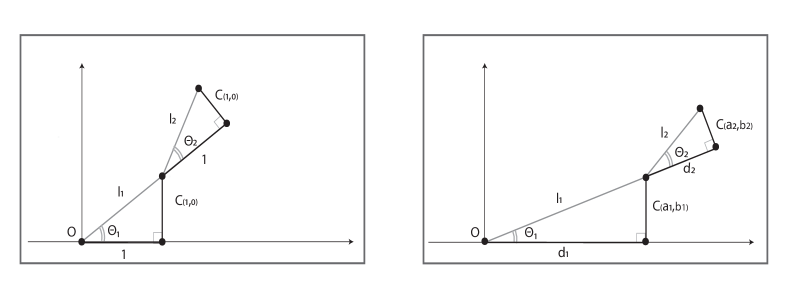
Figure 1: The angular process in the Euclidean plane. By $C_{(a_{j},b_{j})}$ we indicate the j-th random displacement with Cauchy distribution possessing scale parameter $a_{j}$ and location parameter $b_{j}$.

After $n$ steps the sequence of random angles $\Theta_{1},\cdots,\Theta_{n}$ describes the rotation of the moving particle around the starting point, their partial sums describe an angular random walk which can be written as

$${S}_{n}=\Theta_{1}+\cdots+\Theta_{n}=\sum_{j=1}^{n}\arctan{\mathbb{C}}_{j}$$ (1.1)

where ${\mathbb{C}}_{j}$ are independent standard Cauchy random variables. If the random steps of the planar random walk above were independent Cauchy random variables with scale parameter $a_{j}$ and location parameter $b_{j}$ then the process (1.1) must be a little bit modified and rewritten as

$$S_{n}=\Theta_{1}+\cdots+\Theta_{n}=\sum_{j=1}^{n}\arctan C_{j},$$ (1.2)

where $C_{j}\sim C_{(a_{j},b_{j})}$. The model (1.2) can be extended also to the case where the first step has length $d_{j}$ and the second one is Cauchy distributed with scale parameter $a_{j}$ and position parameter $b_{j}$ (see Figure 1), then

$$\tan\Theta_{j}=C_{\left(\frac{a_{j}}{d_{j}},\frac{b_{j}}{d_{j}}\right)}.$$

The same random walk can be generated if the two orthogonal steps, at each displacement, are represented by two independent Gaussian random variables $X_{j}$ and $Y_{j}$. In this case, for each right triangle, we can write

$$\tan\Theta_{j}=\frac{X_{j}}{Y_{j}}.$$

If $X_{j}$ and $Y_{j}$ are two standard independent Gaussian random variables then $\tan\Theta_{j}=\frac{X_{j}}{Y_{j}}$ possesses standard Cauchy distribution and we get the model in (1.1). The model (1.2) can be obtained by considering orthogonal Gaussian steps with different variances and in this case the scale parameter of the random variables $C_{j}$ is the ratio $a_{j}=\sigma_{j}^{Y}/\sigma_{j}^{X}$.

The model (1.1) describing the angular random process has an hyperbolic counterpart. We consider a particle starting from the origin $O$ of the Poincaré half-plane $\mathbb{H}^{2}_{+}=\{(x,y):\;y>0\}$. At the $j$-th displacement, $j=1,2\dots$, the particle makes two steps of random hyperbolic length $\eta_{j}$ and $\hat{\eta}_{j}$ on two orthogonal geodesic lines. The $j$-th displacement leads to a right triangle $T_{j}$ with sides of length $\eta_{j}$ and $\hat{\eta}_{j}$ and random acute angles $\Theta_{j}$ and $\widehat{\Theta}_{j}$. In each triangle $T_{j}$ the first step is taken on the extension of the hypotenuse of the triangle $T_{j-1}$ (see Figure 2). From hyperbolic trigonometry (for basic results on hyperbolic geometry see, for example, Faber [5]) we have that

$$\sin\Theta_{j}=\frac{\sinh\hat{\eta}_{j}}{\sqrt{\cosh^{2}\eta_{j}\cosh^{2}\hat{\eta}_{j}-1}},\;\;\;\;\cos\Theta_{j}=\frac{\sinh\eta_{j}\cosh\hat{\eta}_{j}}{\sqrt{\cosh^{2}\eta_{j}\cosh^{2}\hat{\eta}_{j}-1}}.$$

From the above expressions we have that

$$\tan\Theta_{j}=\frac{\tanh\hat{\eta}_{j}}{\sinh\eta_{j}}.$$

If we take independent random hyperbolic displacements $\eta_{j}$ and $\hat{\eta}_{j}$ such that the random variables $E_{j}=\frac{\tanh\hat{\eta}_{j}}{\sinh\eta_{j}}$ are standard Cauchy distributed then $\Theta_{j}=\arctan{\mathbb{C}}_{j}$. If the triangles $T_{j}$ were isosceles then $\tan\Theta_{j}=\frac{1}{\cosh\eta_{j}}$ and the angle $\Theta_{j}\in[-\frac{\pi}{4},\frac{\pi}{4}]$ so that in this case the Cauchy distribution cannot be attributed to $\tan\Theta_{j}$.

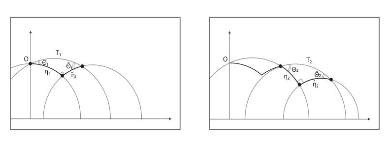
Figure 2: The angular random process in the Poincaré half-plane.

In the model described here the random steps (and therefore the random angular windings $\Theta_{j}$) are independent. If we consider the model of papers [2] and [3], where the displacements are taken orthogonally to the geodesic lines joining the origin $O$ of $\mathbb{H}^{2}_{+}$ with the positions occupied at deviation instants, the angular displacements $\Theta_{j}$ must be such that

$$\sin\Theta_{j}=\frac{\sinh\eta_{j}}{\sqrt{1+\prod_{r=1}^{j}\cosh^{2}\eta_{r}}}=\sinh\eta_{j}\cos\left(\arctan\prod_{r=1}^{j}\cosh^{2}\eta_{r}\right)$$

and therefore involve dependent random variables.

For the area of the random hyperbolic triangle $T_{j}$ we note that

$$\mathrm{area}(T_{j}) = \frac{\pi}{2}-\Theta_{j}-\hat{\Theta}_{j}=\frac{\pi}{2}-\left[\arctan\left(\frac{\tanh\hat{\eta}_{j}}{\sinh\eta_{j}}\right)+\arctan\left(\frac{\tanh\eta_{j}}{\sinh\hat{\eta}_{j}}\right)\right]$$

$$= \frac{\pi}{2}-\arctan\left(\frac{\coth\eta_{j}}{\sinh\hat{\eta}_{j}}+\frac{\coth\hat{\eta}_{j}}{\sinh{\eta}_{j}}\right)=\mathrm{arcotan}\left(\frac{\coth{\eta}_{j}}{\sinh\hat{\eta}_{j}}+\frac{\coth\hat{\eta}_{j}}{\sinh{\eta}_{j}}\right).$$

Since each acute angle inside $T_{j}$ is linked to both sides of the triangle, the analysis of the random process $A_{n}=\sum_{j=1}^{n}\mathrm{area}(T_{j})$ is much more complicated and we drop it.

Let $C_{j}\sim C_{(a_{j},b_{j})}$, $j=1,2\dots$ be independent Cauchy random variables where $a_{j}$ is the scale parameter and $b_{j}$ is the location parameter. In the study of the angular random walk (1.1) and (1.2) we must analyze the distribution of the following non-linear transformations of Cauchy random variables:

$$U=\frac{C_{1}+C_{2}}{1-C_{1}C_{2}}$$ (1.3)

since

$$\arctan C_{1}+\arctan C_{2}=\arctan\frac{C_{1}+C_{2}}{1-C_{1}C_{2}}.$$

Since the Sixties a wide class of non-linear transformations of Cauchy random variables has been considered. Williams [10], Knight [6] and Letac [7] proved that transformations of the form

$$\epsilon f(x)=kx+\alpha-\sum_{i=1}^{n}\frac{\mu_{i}}{x-\gamma_{i}}$$

where $\epsilon=\pm 1$, $\alpha,\gamma_{i}\in\mathbb{R}$ and $k,\mu_{i}\geq 0$ preserve the Cauchy distribution.

In particular, in Williams [10] it is proved the following characterization for Cauchy random variables. The random variable $X$ is a standard Cauchy if and only if $(1+bX)/(b-X)$ is a standard Cauchy for some constant $b$ which is not the tangent of a rational multiple of $\pi$.

Knight [6] asserts that a random variable $X$ is of Cauchy type if and only if the random variable $(aX+b)/(cX+d)$ is still of Cauchy type, whenever $ad-bc\neq 0$.

Our problem is more strictly related to the results obtained by Pitman and Williams [8]. They proved that the standard Cauchy distribution is preserved under certain types of transformations represented by meromorphic functions whose poles are all real and simple. As a corollary they obtained that, if $P$ and $Q$ are two independent random variables uniformly distributed in $(0,\pi)$, then the random variables $X=\tan P$ and $Y=\tan Q$ are standard Cauchy and

$$\tan(P+Q)=\frac{X+Y}{1-XY}\stackrel{{\scriptstyle law}}{{=}}X.$$

We will show that the random variable (1.3) is endowed with Cauchy distribution in a much more general situation, namely when the random variables $C_{j}$, $j=1,2$, have non-zero location parameters $b_{j}$ and scale parameters $a_{j}$. The scale and location parameters of $U$ depend on both parameters $a_{j}$ and $b_{j}$ suitably combined.

In particular, if $b_{1}=b_{2}=0$ and $a_{1}=a_{2}=1$, then $U$ is still distributed as a standard Cauchy distribution and therefore in (1.1) we have that

$${S}_{n}\stackrel{{\scriptstyle law}}{{=}}\arctan{\mathbb{C}}.$$

Since also $\frac{1}{{\mathbb{C}}}$ is a standard Cauchy (for basic properties of Cauchy random variables see, for example, Chaumont and Yor [9] page 105), from (1.3), a number of related random variables preserving the form of the Cauchy distribution can be considered. For example, the following random variables

$$Z_{1}=\frac{{\mathbb{C}}_{1}{\mathbb{C}}_{2}+1}{{\mathbb{C}}_{1}-{\mathbb{C}}_{2}},\;\;\;\;\;\;\;\;Z_{2}=\frac{1-{\mathbb{C}}_{1}{\mathbb{C}}_{2}}{{\mathbb{C}}_{1}+{\mathbb{C}}_{2}},\;\;\;\;\;\;\;\;Z_{3}=\frac{{\mathbb{C}}_{1}+{\mathbb{C}}_{2}}{{\mathbb{C}}_{1}{\mathbb{C}}_{2}-1},$$

also possess standard Cauchy distribution.

If $b_{1}=b_{2}=0$ and the scale parameters $a_{1},a_{2}$ are different, then (1.3) still preserves the Cauchy distribution but with scale parameter equal to $\frac{a_{1}+a_{2}}{1+a_{1}a_{2}}$ and location parameter equal to zero. This can be grasped by means of the following relationship

$$\arctan C_{1}+\arctan C_{2}\stackrel{{\scriptstyle law}}{{=}}\arctan\left\{\frac{a_{1}+a_{2}}{1+a_{1}a_{2}}{\mathbb{C}}\right\},$$ (1.4)

where $C_{j}\sim C_{(a_{j},0)}$. Result (1.4) is illustrated in Figure 3.

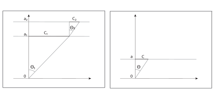
Figure 3: The figure shows that shooting a ray with inclination $\Theta_{1}$, uniformly distributed, against the line at distance $a_{1}$ and then shooting a ray with a uniformly distributed angle $\Theta_{2}$ on the line at distance $a_{2}$ is equivalent to shooting on the barrier at the distance $a=\frac{a_{1}+a_{2}}{1+a_{1}a_{2}}$ with a uniformly distributed angle $\Theta$.

By iterating the process (1.4) we arrive at the formula

$$\sum_{j=1}^{3}\arctan C_{j}\stackrel{{\scriptstyle law}}{{=}}\arctan\left\{\frac{\sum_{j=1}^{3}a_{j}+a_{1}a_{2}a_{3}}{1+\sum_{i\neq j}a_{i}a_{j}}{\mathbb{C}}\right\}$$

which gives an insight into further extensions of the process outlined above.

Much more complicated are the cases where the location parameters of the Cauchy distributions are different from zero. For the special case where $C_{1}$ and $C_{2}$ are independent Cauchy such that $C_{1}\sim C_{(1,b)}$ and $C_{2}\sim C_{(1,b)}$, the random variable (1.3) still possesses Cauchy density with scale parameter $\frac{2b^{2}+4}{b^{4}+4}$ and location parameter $\frac{2b^{3}}{b^{4}+4}$.

We have obtained the general distribution of (1.3) where $C_{1}$ and $C_{2}$ are independent Cauchy such that $C_{1}\sim C_{(a_{1},b_{1})}$ and $C_{2}\sim C_{(a_{2},b_{2})}$ and also the distribution of

$${U}=\frac{\gamma C_{1}+\delta C_{2}}{\alpha-\beta C_{1}C_{2}}$$

for arbitrary positive real numbers $\beta,\gamma,\delta$ and $\alpha+\beta\neq 0$. In particular, if $C_{1}$ and $C_{2}$ are independent standard Cauchy random variables then $U$ is Cauchy with scale parameter equal to $\left|\frac{\gamma+\delta}{\alpha+\beta}\right|$ and location parameter equal to zero.

In the last section we have examined continued fractions involving Cauchy random variables. In particular we have studied

$$V_{n}=\frac{1}{1+\frac{1}{1+\frac{1}{1+\cdots\frac{1}{1+{\mathbb{C}}}}}}$$ (1.5)

and

$$U_{n}=\frac{1}{1+\frac{1}{1+\frac{1}{1+\cdots\frac{1}{1+{\mathbb{C}}^{2}}}}}$$ (1.6)

which generalize the random variables $V_{1}=\frac{1}{1+{\mathbb{C}}}$ and $U_{1}=\frac{1}{1+{\mathbb{C}}^{2}}$. Continued fractions involving random variables have been analyzed in Chamayou and Letac [4] and more recently in Asci, Letac and Piccioni [1]. The random variable $U_{1}$ has the arcsine distribution in $[0,1]$, while $U_{t}=tU_{1}$, with $t>0$, has distribution

$$\mathrm{Pr}\{U_{t}\in ds\}=\frac{\mathrm{d}s}{\pi\sqrt{s(t-s)}},\hskip 28.45274pt0<s<t.$$

For each $n\geq 1$, the random variables $V_{n}$, are Cauchy distributed with scale parameter $a_{n}$ and position parameter $b_{n}$ that can be expressed in terms of Fibonacci numbers. This permits us to prove the monotonicity of $a_{n}$ and $b_{n}$ and that $\lim_{n\to\infty}a_{n}=0$ and $\lim_{n\to\infty}b_{n}=\phi-1$ where $\phi=\frac{1+\sqrt{5}}{2}$ is the golden ratio. Finally we obtain that the sequence of random variables $1+V_{n}$ and $1+U_{n}$, $n\geq 1$, converges in distribution to the number $\phi=\frac{1+\sqrt{5}}{2}$. This should be expected since it has the infinite fractional expansion

$$\frac{1+\sqrt{5}}{2}=1+\frac{1}{1+\frac{1}{1+\cdots}}$$ (1.7)

which is related to (1.5) and (1.6).

2 Centered Cauchy random variables

In this section we study the distribution of the following random variable

$$U=\frac{\gamma{\mathbb{C}}_{1}+\delta{\mathbb{C}}_{2}}{\alpha-\beta{\mathbb{C}}_{1}{\mathbb{C}}_{2}},$$ (2.1)

where ${\mathbb{C}}_{1}$ and ${\mathbb{C}}_{2}$ are independent, standard Cauchy. We assume, without restrictions, that $\beta,\gamma,\delta$ are non-negative real numbers all different from zero (because of the symmetry of ${\mathbb{C}}_{j}$, $j=1,2$) and $\alpha+\beta\neq 0$. In the next theorem we prove that $U$ is still Cauchy distributed.

Theorem 2.1.

The random variable $U$ in (2.1) possesses Cauchy distribution with scale parameter equal to $\left|\frac{\gamma+\delta}{\alpha+\beta}\right|$ and position parameter equal to zero. We can also restate the result in symbols as

$$U\stackrel{{\scriptstyle law}}{{=}}\frac{\gamma+\delta}{\alpha+\beta}{\mathbb{C}}.$$

Proof 1
The density of the random variable $U$ can be obtained by means of the transformation

$$\left\{\begin{array}[]{lr}u=\frac{\gamma x+\delta y}{\alpha-\beta xy},\\ v=y,\end{array}\right.$$

with $(x,y)\in\mathbb{R}^{2}$ and Jacobian equal to

$$|J|=\frac{\alpha\gamma+\delta\beta v^{2}}{(\gamma+\beta uv)^{2}}.$$

The joint density $g=g(u,v)$ reads

$$g(u,v) = \frac{1}{\pi^{2}(1+v^{2})}\frac{1}{1+\left(\frac{\alpha u-\delta v}{\gamma+\beta uv}\right)^{2}}\frac{\alpha\gamma+\delta\beta v^{2}}{(\gamma+\beta uv)^{2}}\hskip 28.45274pt(u,v)\in\mathbb{R}^{2}$$

$$= \frac{1}{\pi^{2}(1+v^{2})}\frac{\alpha\gamma+\delta\beta v^{2}}{v^{2}(\beta^{2}u^{2}+\delta^{2})+2uv(\beta\gamma-\delta\alpha)+\alpha^{2}u^{2}+\gamma^{2}}$$

and must be integrated with respect to $v$ in order to obtain the distribution of $U$. Therefore

$$\mathrm{Pr}\left\{\frac{\gamma{\mathbb{C}}_{1}+\delta{\mathbb{C}}_{2}}{\alpha-\beta{\mathbb{C}}_{1}{\mathbb{C}}_{2}}\in\mathrm{d}u\right\} = \frac{\mathrm{d}u}{\pi^{2}}\int_{-\infty}^{\infty}\left[\frac{1}{1+v^{2}}\frac{\alpha\gamma+\delta\beta v^{2}}{v^{2}(u^{2}\beta^{2}+\delta^{2})+2vu(\beta\gamma-\delta\alpha)+u^{2}\alpha^{2}+\gamma^{2}}\right]\mathrm{d}v$$

$$= \frac{\mathrm{d}u}{\pi^{2}}\int_{-\infty}^{\infty}\left[\frac{Av+B}{1+v^{2}}+\frac{Cv+D}{v^{2}(u^{2}\beta^{2}+\delta^{2})+2vu(\beta\gamma-\delta\alpha)+u^{2}\alpha^{2}+\gamma^{2}}\right]\mathrm{d}v$$

where

$$\left\{\begin{array}[]{lr}\vspace{0.3cm}A=\frac{2u(\beta\gamma-\alpha\delta)(\beta\delta-\alpha\gamma)}{[u^{2}(\alpha-\beta)^{2}+(\gamma-\delta)^{2}][u^{2}(\alpha+\beta)^{2}+(\gamma+\delta)^{2}]},\\ \vspace{0.3cm}B=\frac{(\alpha\gamma-\beta\delta)[(\gamma^{2}-\delta^{2})+u^{2}(\alpha^{2}-\beta^{2})]}{[u^{2}(\alpha-\beta)^{2}+(\gamma-\delta)^{2}][u^{2}(\alpha+\beta)^{2}+(\gamma+\delta)^{2}]},\\ \vspace{0.3cm}C=-A(u^{2}\beta^{2}+\delta^{2}),\\ \vspace{0.3cm}D=\frac{(\beta\gamma-\alpha\delta)[u^{4}\alpha\beta(\beta^{2}-\alpha^{2})+u^{2}(\beta\gamma-\alpha\delta)(3\alpha\gamma-\beta\delta)+\gamma\delta(\gamma^{2}-\delta^{2})]}{[u^{2}(\alpha-\beta)^{2}+(\gamma-\delta)^{2}][u^{2}(\alpha+\beta)^{2}+(\gamma+\delta)^{2}]}.\end{array}\right.$$

We start by evaluating the first part of the integral (2):

$$\int_{-\infty}^{\infty}\left[\frac{Av}{1+v^{2}}+\frac{Cv}{v^{2}(u^{2}\beta^{2}+\delta^{2})+2vu(\beta\gamma-\delta\alpha)+u^{2}\alpha^{2}+\gamma^{2}}\right]\mathrm{d}v$$ (2.3)

$$= \frac{A}{2}\int_{-\infty}^{\infty}\left[\frac{2v}{1+v^{2}}-\frac{2v(u^{2}\beta^{2}+\delta^{2})\pm 2u(\beta\gamma-\delta\alpha)}{v^{2}(u^{2}\beta^{2}+\delta^{2})+2vu(\beta\gamma-\delta\alpha)+u^{2}\alpha^{2}+\gamma^{2}}\right]\mathrm{d}v$$

$$= \frac{A}{2}\left.\lim_{d\to\infty,c\to-\infty}\log\left(\frac{1+v^{2}}{v^{2}(u^{2}\beta^{2}+\delta^{2})+2vu(\beta\gamma-\delta\alpha)+u^{2}\alpha^{2}+\gamma^{2}}\right)\right|_{c}^{d}$$

$$+Au(\beta\gamma-\delta\alpha)\int_{-\infty}^{\infty}\frac{1}{v^{2}(u^{2}\beta^{2}+\delta^{2})+2vu(\beta\gamma-\delta\alpha)+u^{2}\alpha^{2}+\gamma^{2}}\mathrm{d}v$$

$$= Au(\beta\gamma-\delta\alpha)\int_{-\infty}^{\infty}\frac{1}{v^{2}(u^{2}\beta^{2}+\delta^{2})+2vu(\beta\gamma-\delta\alpha)+u^{2}\alpha^{2}+\gamma^{2}}\mathrm{d}v$$

$$= Au(\beta\gamma-\delta\alpha)\frac{\pi}{u^{2}\alpha\beta+\gamma\delta},$$

where the last integral is obtained by means of the change of variable

$$v\sqrt{u^{2}\beta^{2}+\delta^{2}}+\frac{u(\beta\gamma-\delta\alpha)}{\sqrt{u^{2}\beta^{2}+\delta^{2}}}=z\sqrt{u^{2}\alpha^{2}+\gamma^{2}-\frac{u^{2}(\beta\gamma-\delta\alpha)^{2}}{u^{2}\beta^{2}+\delta^{2}}}=z\frac{u^{2}\alpha\beta+\gamma\delta}{\sqrt{u^{2}\beta^{2}+\delta^{2}}}.$$

In view of result (2.3) and inserting the values of $A$, $B$ and $D$ we have that

$$\frac{\mathrm{d}u}{\pi^{2}}\int_{-\infty}^{\infty}\left[\frac{Av+B}{1+v^{2}}+\frac{Cv+D}{v^{2}(u^{2}\beta^{2}+\delta^{2})+2vu(\beta\gamma-\delta\alpha)+u^{2}\alpha^{2}+\gamma^{2}}\right]\mathrm{d}v$$

$$= \frac{\mathrm{d}u}{\pi}\frac{1}{u^{2}\alpha\beta+\gamma\delta}[Au(\beta\gamma-\alpha\delta)+B(u^{2}\alpha\beta+\gamma\delta)+D]$$

$$= \frac{\mathrm{d}u}{\pi}\left[\frac{(\gamma\delta+u^{2}\alpha\beta)(\beta\gamma-\alpha\delta)[u^{2}(\beta^{2}-\alpha^{2})+(\gamma^{2}-\delta^{2})]}{(u^{2}\alpha\beta+\gamma\delta)[u^{2}(\alpha-\beta)^{2}+(\gamma-\delta)^{2}][u^{2}(\alpha+\beta)^{2}+(\gamma+\delta)^{2}]}\right.$$

$$+\left.\frac{(\gamma\delta+u^{2}\alpha\beta)(\alpha\gamma-\beta\delta)[u^{2}(\alpha^{2}-\beta^{2})+(\gamma^{2}-\delta^{2})]}{(u^{2}\alpha\beta+\gamma\delta)[u^{2}(\alpha-\beta)^{2}+(\gamma-\delta)^{2}][u^{2}(\alpha+\beta)^{2}+(\gamma+\delta)^{2}]}\right]$$

$$= \frac{\mathrm{d}u}{\pi}\frac{u^{2}(\beta^{2}-\alpha^{2})(\beta-\alpha)(\gamma+\delta)+(\gamma^{2}-\delta^{2})(\alpha+\beta)(\gamma-\delta)}{[u^{2}(\alpha-\beta)^{2}+(\gamma-\delta)^{2}][u^{2}(\alpha+\beta)^{2}+(\gamma+\delta)^{2}]}$$

$$= \frac{\mathrm{d}u}{\pi}\frac{(\alpha+\beta)(\gamma+\delta)[u^{2}(\alpha-\beta)^{2}+(\gamma-\delta)^{2}]}{[u^{2}(\alpha-\beta)^{2}+(\gamma-\delta)^{2}][u^{2}(\alpha+\beta)^{2}+(\gamma+\delta)^{2}]}$$

$$= \frac{\mathrm{d}u}{\pi}\frac{(\alpha+\beta)(\gamma+\delta)}{u^{2}(\alpha+\beta)^{2}+(\gamma+\delta)^{2}}.$$

Another approach is based on the conditional characteristic function,

$$\mathrm{E}\{e^{i\beta U}|\mathbb{C}_{2}=v\} = \frac{1}{\pi}\int_{-\infty}^{\infty}e^{i\beta(\frac{\gamma u+\delta v}{\alpha-\beta uv})}\frac{\mathrm{d}u}{1+u^{2}}$$

$$= \frac{1}{\pi}\int_{-\infty}^{\infty}e^{i\beta w}\frac{\alpha\gamma+\delta\beta v^{2}}{v^{2}(\beta^{2}w^{2}+\delta^{2})+2vw(\beta\gamma-\delta\alpha)+w^{2}\alpha^{2}+\gamma^{2}}\mathrm{d}w$$

where $w=\frac{\gamma u+\delta v}{\alpha-\beta uv}$. The inverse Fourier transform gives the conditional density $g(w|v)$ and thus we arrive again at the integral (2).

$\blacksquare$

Remark 2.1.

A special case implied by Theorem 2.1 concerns the random variable

$$V=\frac{C_{1}+C_{2}}{1-C_{1}C_{2}}$$

where $C_{j}\sim C_{(a_{j},0)}$, with $j=1,2$, are independent Cauchy random variables with location parameter equal to zero and scale parameter $a_{j}>0$. If we choose $\gamma=a_{1}$, $\delta=a_{2}$, $\alpha=1$ and $\beta=a_{1}a_{2}$, we conclude that

$$V\stackrel{{\scriptstyle law}}{{=}}\frac{a_{1}{\mathbb{C}}_{1}+a_{2}{\mathbb{C}}_{1}}{1-a_{1}a_{2}{\mathbb{C}}_{1}{\mathbb{C}}_{2}}\stackrel{{\scriptstyle law}}{{=}}\frac{a_{1}+a_{2}}{1+a_{1}a_{2}}{\mathbb{C}}.$$

In the same way we obtain that

$$\widehat{V}=\frac{\gamma C_{1}+\delta C_{2}}{\alpha-\beta C_{1}C_{2}}\stackrel{{\scriptstyle law}}{{=}}\frac{\gamma a_{1}{\mathbb{C}}_{1}+\delta a_{2}{\mathbb{C}}_{2}}{\alpha-\beta a_{1}a_{2}{\mathbb{C}}_{1}{\mathbb{C}}_{2}}\stackrel{{\scriptstyle law}}{{=}}\frac{\gamma a_{1}+\delta a_{2}}{\alpha+\beta a_{1}a_{2}}{\mathbb{C}}.$$

where $\alpha+\beta a_{1}a_{2}\neq 0$.

Remark 2.2.

In view of Theorem 2.1 we can obtain by recurrence the distribution of the current angle after $n$ steps for the angular random walk

$$S_{n}=\sum_{j=1}^{n}\arctan C_{j}$$

described in the introduction. We have

$$S_{n}=\sum_{j=1}^{n}\arctan C_{j(a_{j},0)}=\arctan C_{(\hat{a}_{n-1},0)}+\arctan C_{n}(a_{n},0)$$

where $\arctan C(\hat{a}_{n-1},0)$ is the random variable $S_{n-1}$. In particular, if $a_{j}=1$ for $j=1,\dots n$, we have the following property of the standard Cauchy random variables ${\mathbb{C}}_{j}$

$$\sum_{j=1}^{n}\arctan{\mathbb{C}}_{j}\stackrel{{\scriptstyle law}}{{=}}\arctan{\mathbb{C}}.$$

Remark 2.3.

A simple byproduct of Theorem 2.1 is that

$$Ee^{i\beta U} = \frac{1}{\pi^{2}}\int_{\mathbb{R}^{2}}e^{i\beta\frac{x+y}{1-xy}}\frac{a_{1}a_{2}\mathrm{d}x\mathrm{d}y}{(a_{1}^{2}+x^{2})(a_{2}^{2}+y^{2})}=\frac{1}{\pi^{2}}\int_{-\frac{\pi}{2}}^{\frac{\pi}{2}}\int_{-\frac{\pi}{2}}^{\frac{\pi}{2}}e^{i\beta\frac{a_{1}\tan\theta_{1}+a_{2}\tan\theta_{2}}{1-a_{1}a_{2}\tan\theta_{1}\tan\theta_{2}}}\mathrm{d}\theta_{1}\mathrm{d}\theta_{2}$$ (2.4)

$$= e^{-\frac{a_{1}+a_{2}}{1+a_{1}a_{2}}|\beta|}.$$

In (2.4) we have used the transformations $x=a_{1}\tan\theta_{1}$ and $y=a_{2}\tan\theta_{2}$. In the special case $a_{1}=a_{2}=1$ the relationship (2.4) yields

$$e^{-|\beta|} = \frac{1}{\pi^{2}}\int_{-\frac{\pi}{2}}^{\frac{\pi}{2}}\int_{-\frac{\pi}{2}}^{\frac{\pi}{2}}e^{i\beta\frac{\tan\theta_{1}+\tan\theta_{2}}{1-\tan\theta_{1}\tan\theta_{2}}}\mathrm{d}\theta_{1}\mathrm{d}\theta_{2}=\frac{1}{\pi^{2}}\int_{-\frac{\pi}{2}}^{\frac{\pi}{2}}\int_{-\frac{\pi}{2}}^{\frac{\pi}{2}}e^{i\beta\tan(\theta_{1}+\theta_{2})}\mathrm{d}\theta_{1}\mathrm{d}\theta_{2}$$ (2.5)

$$= \frac{2}{\pi^{2}}\int_{0}^{\pi}x\cos(\beta\tan x)\mathrm{d}x.$$

In the last step of (2.5) we have used the transformations $\theta_{1}+\theta_{2}=x$ and $\theta_{2}=y$. The integral (2.5) shows that, if $(\Theta_{1},\Theta_{2})$ is uniform in the square $S=\{(\theta_{1},\theta_{2}):-\frac{\pi}{2}<|\theta_{i}|<\frac{\pi}{2},\;i=1,2\}$, then the random variable $W=\tan(\Theta_{1}+\Theta_{2})$ has characteristic function $e^{-|\beta|}$ because $\Theta_{1}+\Theta_{2}$ is uniform and therefore $W$ is Cauchy distributed.

Remark 2.4.

It is well-known that for a planar Brownian motion $\{(B_{1}(t),B_{2}(t)),t>0\}$ starting from $(x,y)$ the random variable $B_{1}(T_{y})$ possesses Cauchy distribution with parameters $(x,y)$ where

$$T_{y}=\inf\{t>0:\;B_{2}(t)=0\}.$$

If the starting points of two planar Brownian motions $(B^{i}_{1}(t),B^{i}_{2}(t))$, for $i=1,2$, are located on the $y$ axis as in the Figure 4 then we have that

$$\Theta=\Theta_{1}+\Theta_{2} = \arctan B^{1}_{1}(T_{a_{1}})+\arctan B^{2}_{1}(T_{a_{2}})$$

$$\stackrel{{\scriptstyle law}}{{=}} \arctan C_{1}+\arctan C_{2}$$

$$\stackrel{{\scriptstyle law}}{{=}} \arctan\frac{a_{1}+a_{2}}{1+a_{1}a_{2}}{\mathbb{C}}.$$

where $C_{1}$ and $C_{2}$ are two independent Cauchy random variables with scale parameters $a_{1}$ and $a_{2}$ respectively and position parameter equal to zero. Therefore if the starting point of a third Brownian motion has coordinates $\left(0,\frac{a_{1}+a_{2}}{1+a_{1}a_{2}}\right)$ then $B\left(T_{\frac{a_{1}+a_{2}}{1+a_{1}a_{2}}}\right)$ represents its hitting position on the $x$-axis. This point forms with $(0,1)$ and the origin a right triangle with an angle equal to $\Theta=\Theta_{1}+\Theta_{2}$.

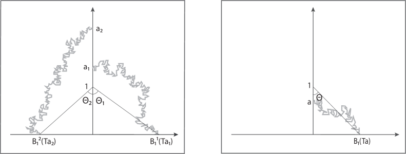
Figure 4: The hitting position on the $x$-axis of a planar Brownian motion is Cauchy distributed. In the figure the random angles $\Theta_{1}$, $\Theta_{2}$ and $\Theta=\Theta_{1}+\Theta_{2}$ are shown. For $a=\frac{a_{1}+a_{2}}{1+a_{1}a_{2}}$ the right-hand figure shows the hitting position $B_{1}(T_{a})$.

3 Non-Centered Cauchy random variables

For independent Cauchy random variables $C_{1}$ and $C_{2}$, with location parameters $b_{1}$ and $b_{2}$ and scale parameters $a_{1}$ and $a_{2}$, the random variable $U$ in (2.1) is still Cauchy distributed with both parameters affected by the values of the location parameters $b_{1}$, $b_{2}$ and the scale parameters $a_{1}$, $a_{2}$.

Theorem 3.1.

If $C_{i}$, $i=1,2$, are two independent, Cauchy random variables with location parameters $b_{i}$ and scale parameters $a_{i}$, then the random variable $U$ is still Cauchy distributed with scale parameter

$$a_{U}=\frac{(a_{1}+a_{2})(1+a_{1}a_{2}-b_{1}b_{2})+(b_{1}+b_{2})(a_{1}b_{2}+a_{2}b_{1})}{(1+a_{1}a_{2}-b_{1}b_{2})^{2}+(a_{1}b_{2}+a_{2}b_{1})^{2}},$$

and position parameter

$$b_{U}=\frac{(a_{1}+a_{2})(a_{1}b_{2}+a_{2}b_{1})-(b_{1}+b_{2})(1+a_{1}a_{2}-b_{1}b_{2})}{(1+a_{1}a_{2}-b_{1}b_{2})^{2}+(a_{1}b_{2}+a_{2}b_{1})^{2}}.$$

Proof
We obtain the density function of the random variable $U$ by observing that

$$\mathrm{Pr}\{U\in\mathrm{d}w\}=\mathrm{E}\left\{\mathrm{Pr}\left\{\left.\frac{C_{1}+C_{2}}{1-C_{1}C_{2}}\in\mathrm{d}w\right|C_{2}\right\}\right\}$$

and remarking that

$$\mathrm{Pr}\left\{\left.\frac{C_{1}+C_{2}}{1-C_{1}C_{2}}\in\mathrm{d}w\right|C_{2}=y\right\}=\frac{a_{1}}{\pi\left[\frac{w-y}{1+wy}-b_{1}\right]^{2}+a_{1}^{2}}\frac{1+y^{2}}{(1+wy)^{2}}\mathrm{d}w.$$

Therefore

$$\mathrm{Pr}\{U\in\mathrm{d}w\} = \frac{a_{1}a_{2}\;\mathrm{d}w}{\pi^{2}}\int_{-\infty}^{\infty}\frac{1}{\left[\frac{w-y}{1+wy}-b_{1}\right]^{2}+a_{1}^{2}}\frac{1+y^{2}}{(1+wy)^{2}}\frac{1}{(y-b_{2})^{2}+a_{2}^{2}}\mathrm{d}y$$ (3.1)

$$= \frac{a_{1}a_{2}\;\mathrm{d}w}{\pi^{2}}\int_{-\infty}^{\infty}\frac{1+y^{2}}{\left[w-y-b_{1}(1+wy)\right]^{2}+a_{1}^{2}(1+wy)^{2}}\frac{1}{(y-b_{2})^{2}+a_{2}^{2}}\mathrm{d}y$$

$$= \frac{a_{1}a_{2}\;\mathrm{d}w}{\pi^{2}}\int_{-\infty}^{\infty}\frac{1+y^{2}}{[y^{2}E-2yF+G][y^{2}-2yH+K]}\mathrm{d}y,$$

where

$$E=1+2b_{1}w+(a_{1}^{2}+b_{1}^{2})w^{2},\hskip 28.45274ptF=-b_{1}-(a_{1}^{2}+b_{1}^{2}-1)w+b_{1}w^{2},$$

$$G=a_{1}^{2}+b_{1}^{2}-2b_{1}w+w^{2},\hskip 28.45274ptH=b_{2},\hskip 28.45274ptK=a_{2}^{2}+b_{2}^{2}.$$

We rewrite the integral in (3.1) in the following form

$$\mathrm{Pr}\{U\in\mathrm{d}w\} = \frac{a_{1}a_{2}\;\mathrm{d}w}{\pi^{2}}\int_{-\infty}^{\infty}\left[\frac{Ay+B}{y^{2}E-2yF+G}+\frac{Cy+D}{y^{2}-2yH+K}\right]\mathrm{d}y$$ (3.2)

with

$$\left\{\begin{array}[]{lr}A+CE=0,\\ -2AH+B-2CF+DE=1,\\ AK-2HB+CG-2DF=0,\\ BK+DG=1.\end{array}\right.$$ (3.3)

The integrals in (3.2) can be worked out by means of the change of variables

$$y\sqrt{E}-\frac{F}{\sqrt{E}}=x\sqrt{G-\frac{F^{2}}{E}},\hskip 28.45274pty-H=x\sqrt{K-H^{2}}.$$

The first integral becomes

$$\int_{-\infty}^{\infty}\frac{Ay+B}{\left(y\sqrt{E}-\frac{F}{\sqrt{E}}\right)^{2}+G-\frac{F^{2}}{E}}\mathrm{d}y=\int_{-\infty}^{\infty}\frac{1}{E}\frac{BE+AF+xA\sqrt{GE-F^{2}}}{(x^{2}+1)\sqrt{GE-F^{2}}}\mathrm{d}x,$$

and the second one takes the form

$$\int_{-\infty}^{\infty}\frac{Cy+D}{\left(y-H\right)^{2}+K-H^{2}}\mathrm{d}y=\int_{-\infty}^{\infty}\frac{D+CH+xC\sqrt{K-H^{2}}}{(x^{2}+1)\sqrt{K-H^{2}}}\mathrm{d}x.$$

A substantial simplification can be obtained because

$$\sqrt{GE-F^{2}}=a_{1}(1+w^{2}),\hskip 28.45274pt\sqrt{H-K^{2}}=a_{2}.$$

If we turn back to the distribution (3.2), in view of the above calculations, we have that

$$\mathrm{Pr}\{U\in\mathrm{d}w\} = \frac{a_{2}\mathrm{d}w}{\pi^{2}(1+w^{2})E}\int_{-\infty}^{\infty}\frac{BE+AF+xAa_{1}(1+w^{2})}{x^{2}+1}\mathrm{d}x$$

$$+\frac{a_{1}\mathrm{d}w}{\pi^{2}}\int_{-\infty}^{\infty}\frac{D+CH+xCa_{2}}{1+x^{2}}\mathrm{d}x.$$

We observe that, in view of the first equation of (3.3), we have that

$$\frac{a_{1}a_{2}\;\mathrm{d}w}{\pi^{2}}\left(\frac{A}{E}+C\right)\int_{-\infty}^{\infty}\frac{x}{1+x^{2}}\mathrm{d}x=0$$

and

$$\mathrm{Pr}\{U\in\mathrm{d}w\} = \left\{a_{2}\frac{BE+AF}{\pi E(1+w^{2})}+a_{1}\frac{D+CH}{\pi}\right\}\mathrm{d}w$$

$$= \left\{a_{2}\frac{B-CF}{\pi(1+w^{2})}+a_{1}\frac{D+CH}{\pi}\right\}\mathrm{d}w.$$

The values of $B$, $C$ and $D$ can be derived by solving the system (3.3), simplified as

$$\left\{\begin{array}[]{lr}B+2C(HE-F)+DE=1,\\ -2BH+C(G-EK)-2DF=0,\\ BK+DG=1.\end{array}\right.$$

By means of cumbersome computations we arrive at the final result

$$\mathrm{Pr}\{U\in\mathrm{d}w\}$$

$$=\frac{1}{\pi}\frac{(1+a_{1}a_{2}-b_{1}b_{2})[w(a_{1}b_{2}+a_{2}b_{1})+a_{1}+a_{2}]-(a_{1}b_{2}+a_{2}b_{1})[w(1+a_{1}a_{2}-b_{1}b_{2})-(b_{1}+b_{2})]}{[w(1+a_{1}a_{2}-b_{1}b_{2})-(b_{1}+b_{2})]^{2}+[w(a_{1}b_{2}+a_{2}b_{1})+a_{1}+a_{2}]^{2}}$$

$$=\frac{\frac{(a_{1}+a_{2})(1+a_{1}a_{2}-b_{1}b_{2})+(b_{1}+b_{2})(a_{1}b_{2}+a_{2}b_{1})}{(1+a_{1}a_{2}-b_{1}b_{2})^{2}+(a_{1}b_{2}+a_{2}b_{1})^{2}}}{\left[w+\frac{(a_{1}+a_{2})(a_{1}b_{2}+a_{2}b_{1})-(b_{1}+b_{2})(1+a_{1}a_{2}-b_{1}b_{2})}{(1+a_{1}a_{2}-b_{1}b_{2})^{2}+(a_{1}b_{2}+a_{2}b_{1})^{2}}\right]^{2}+\left[\frac{(a_{1}+a_{2})(1+a_{1}a_{2}-b_{1}b_{2})+(b_{1}+b_{2})(a_{1}b_{2}+a_{2}b_{1})}{(1+a_{1}a_{2}-b_{1}b_{2})^{2}+(a_{1}b_{2}+a_{2}b_{1})^{2}}\right]^{2}}.$$

$\blacksquare$

Remark 3.1.

In view of Theorem 3.1 it is possible to obtain the following particular cases.

• For $a_{1}=a_{2}=1$ and $b_{1}=b_{2}=b$, we have that

  $$a_{U}=\frac{2b^{2}+4}{b^{4}+4},\hskip 56.9055ptb_{U}=\frac{2b^{3}}{b^{4}+4}.$$

This shows that $U$ has center of symmetry on the positive half-line if $b>0$ and on the negative half-line if $b<0$, therefore the non linear transformation $U$ preserves the sign of the mode.

• For $a_{1}=a_{2}=a$ and $b_{1}=b_{2}=b$ we have that

  $$a_{U}=\frac{2a(1+a^{2}+b^{2})}{(1+a^{2}-b^{2})^{2}+(2ab)^{2}},\hskip 28.45274ptb_{U}=\frac{2b(a^{2}+b^{2}-1)}{(1+a^{2}-b^{2})^{2}+(2ab)^{2}}.$$

We note that $a_{U}$ and $b_{U}$ depend simultaneously from the scale and location parameters of the random variables involved in $U$.

4 Continued Fractions

The property that the reciprocal of a Cauchy random variable has still a Cauchy distribution has a number of possible extensions which we deal with in this section.

We start by considering the sequence

$$V_{1}=\frac{1}{1+{\mathbb{C}}},\hskip 28.45274ptV_{2}=\frac{1}{1+\frac{1}{1+{\mathbb{C}}}},\dots\hskip 28.45274ptV_{n}=\frac{1}{1+\frac{1}{1+\dots\frac{1}{1+{\mathbb{C}}}}},$$ (4.1)

and show the following theorem.

Theorem 4.1.

The random variables defined in (4.1) have Cauchy distribution $V_{n}\sim C_{(a_{n},b_{n})}$ where the scale parameters $a_{n}$ and the location parameters $b_{n}$ satisfy the recursive relationships

$$a_{n+1}=\frac{a_{n}}{(1+b_{n})^{2}+a_{n}^{2}},\hskip 56.9055ptn=1,2,\dots$$ (4.2)

and

$$b_{n+1}=\frac{b_{n}+1}{(1+b_{n})^{2}+a_{n}^{2}},\hskip 56.9055ptn=1,2,\dots$$ (4.3)

Proof
Let us assume that $V_{n}$ possesses Cauchy density with parameters $a_{n}$ and $b_{n}$, therefore $V_{n+1}$ writes

$$\mathrm{Pr}\{V_{n+1}<v\}=\mathrm{Pr}\left\{\frac{1}{1+V_{n}}<v\right\}=\mathrm{Pr}\left\{\frac{1}{1+a_{n}+b_{n}{\mathbb{C}}}<v\right\}.$$

After some computations the density of $V_{n+1}$ can be written as

$$f_{V_{n+1}}(v)=\frac{\frac{a_{n}}{(1+b_{n})^{2}+a_{n}^{2}}}{\pi\left[v-\frac{b_{n}+1}{(1+b_{n})^{2}+a_{n}^{2}}\right]^{2}+\frac{a_{n}^{2}}{[(1+b_{n})^{2}+a_{n}^{2}]^{2}}},\hskip 28.45274ptv\in\mathbb{R}.$$

It can be directly ascertained that $V_{1}$ possesses Cauchy distribution with parameters $a_{1}=1/2$ and $b_{1}=1/2$. $\blacksquare$

Remark 4.1.

We have evaluated the following table of parameters $a_{n}$ and $b_{n}$:

$$\hskip 5.69046ptn\hskip 42.67912pt1\hskip 42.67912pt2\hskip 42.67912pt3\hskip 42.67912pt\dots\hskip 42.67912pt10^{2}$$

$$\hskip 8.5359pta_{n}\hskip 31.2982pt1/2\hskip 34.14322pt1/5\hskip 34.14322pt1/13\hskip 28.45274pt\dots\hskip 28.45274pt5.77e^{-42}$$

$$\hskip 8.5359ptb_{n}\hskip 31.2982pt1/2\hskip 34.14322pt3/5\hskip 34.14322pt8/13\hskip 28.45274pt\dots\hskip 28.45274pt0.618034$$

For $n=1,2,3$ we can observe that the scale parameters $a_{n}$ coincide with the inverse of the odd-indexed Fibonacci numbers while the sequence $b_{n}$ has the numerators coinciding with the even-indexed Fibonacci numbers and the denominators correspond to the odd-indexed Fibonacci numbers.

In light of the previous considerations we can show that for $n\geq 1$

$$b_{n}=\frac{F_{2n}}{F_{2n+1}},\hskip 56.9055pta_{n}=\frac{1}{F_{2n+1}},$$ (4.4)

where $F_{n}$, $n\geq 0$ is the Fibonacci sequence. Recalling that the Fibonacci numbers admit the following representation (it can be easily checked by induction)

$$F_{n}=\frac{\phi^{n}-(1-\phi)^{n}}{\sqrt{5}}$$ (4.5)

where $\phi=\frac{1+\sqrt{5}}{2}$ is the golden ratio, we now prove that if $a_{n}$ and $b_{n}$ have the representation (4.4), then also $a_{n+1}$ and $b_{n+1}$ can be expressed in the same form. From (4.2) and (4.3) we have

$$b_{n+1} = \frac{\frac{F_{2n}}{F_{2n+1}}+1}{\left(\frac{F_{2n}}{F_{2n+1}}+1\right)^{2}+\frac{1}{F^{2}_{2n+1}}}=\frac{F_{2n+2}F_{2n+1}}{F^{2}_{2n+2}+1}$$

$$= F_{2n+2}\left[\frac{\phi^{2n+1}-(1-\phi)^{2n+1}}{\phi^{4n+4}+(1-\phi)^{4n+4}-2\phi^{2n+2}(1-\phi)^{2n+2}+5}\right]\sqrt{5}$$

$$= F_{2n+2}\left[\frac{\phi^{2n+1}-(1-\phi)^{2n+1}}{\left[\phi^{2n+1}-(1-\phi)^{2n+1}\right]\left[\phi^{2n+3}-(1-\phi)^{2n+3}\right]}\right]\sqrt{5}$$

$$= \frac{F_{2n+2}}{F_{2n+3}}.$$

Similar calculations prove that $a_{n+1}=\frac{1}{F_{2n+3}}$. In view of representation (4.4) and (4.5), it is easy to show that

$$\lim_{n\to\infty}b_{n}=\lim_{n\to\infty}\frac{F_{2n}}{F_{2n+1}}=\lim_{n\to\infty}\frac{1-\left(\frac{1-\phi}{\phi}\right)^{2n}}{\phi-(1-\phi)\left(\frac{1-\phi}{\phi}\right)^{2n}}=\frac{1}{\phi}=\phi-1,\hskip 28.45274pt\lim_{n\to\infty}a_{n}=\lim_{n\to\infty}\frac{1}{F_{2n+1}}=0.$$

Otherwise, observing that the sequence $b_{n}$, $n\geq 1$ is increasing, because

$$\frac{b_{n+1}}{b_{n}}=\frac{F_{2n+2}F_{2n+1}}{F_{2n+3}F_{2n}}=\frac{\phi^{4n+3}+(1-\phi)^{4n+3}+1}{\phi^{4n+3}+(1-\phi)^{4n+3}-4}\geq 1$$

and taking the limits in (4.2) and (4.3) we have that

$$L=\frac{L}{(1+H)^{2}+L^{2}},\hskip 56.9055ptH=\frac{H+1}{(1+H)^{2}+L^{2}},$$ (4.6)

where $H=\lim_{n\to\infty}a_{n}$ and $L=\lim_{n\to\infty}b_{n}$. From the relationships in (4.6) we derive the equality

$$\frac{L}{H}=\frac{L}{H+1}$$

that implies $L=0$. In fact, for $L\neq 0$, we arrive at the absurd that $H=H+1$. Substituting $L=0$ in the second formula of (4.6) we obtain

$$H=\frac{1}{H+1},$$

since $H$ satisfies the algebraic equation $H^{2}+H-1=0$ it follows that $H=\phi-1$ where $\phi$ is the golden ratio (see Figure 5).

Remark 4.2.

A slightly more general case concerns the sequence

$$W_{1}=\frac{1}{c_{1}+d_{1}C_{(a_{0},b_{0})}}=\frac{1}{c_{1}+a_{0}d_{1}+b_{0}d_{1}{\mathbb{C}}},\hskip 14.22636ptW_{2}=\frac{1}{c_{2}+d_{2}W_{1}},\hskip 14.22636ptW_{3}=\frac{1}{c_{3}+d_{3}W_{2}},\dots$$

By performing calculations similar to those of Theorem 4.1 we have that $W_{1}$ has Cauchy distribution with scale parameter $a_{1}$ and position parameter $b_{1}$ such that

$$a_{1}=\frac{d_{1}a_{0}}{(c_{1}+d_{1}b_{0})^{2}+d_{1}^{2}a_{0}^{2}},\hskip 14.22636ptb_{1}=\frac{c_{1}+d_{1}b_{0}}{(c_{1}+d_{1}b_{0})^{2}+d_{1}^{2}a_{0}^{2}}.$$

Similarly, if $W_{n}\sim C_{(a_{n},b_{n})}$, than $W_{n+1}\sim C_{(a_{n+1},b_{n+1})}$ where

$$a_{n+1}=\frac{d_{n+1}a_{n}}{(c_{n+1}+d_{n+1}b_{n})^{2}+d_{n+1}^{2}a_{n}^{2}},\hskip 14.22636ptb_{n+1}=\frac{c_{n+1}+d_{n+1}b_{n}}{(c_{n+1}+d_{n+1}b_{n})^{2}+d_{n+1}^{2}a_{n}^{2}}$$ (4.7)

for every $n\geq 2$. The sequences in (4.7) for $c_{n}=d_{n}=1$ coincide with (4.2) and (4.3).

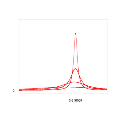
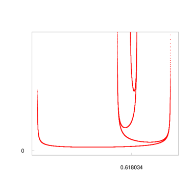
Figure 5: In the left figure the densities of the Cauchy random variables $V_{1}$, $V_{2}$, $V_{3}$ and $V_{4}$ are shown. In the right figure the densities of $U_{1}$, $U_{2}$, $U_{3}$ and $U_{4}$ are plotted.

Another sequence of continued fractions involving the Cauchy distribution is the following one

$$U_{1}=\frac{1}{1+{\mathbb{C}}^{2}},\hskip 28.45274ptU_{2}=\frac{1}{1+\frac{1}{1+{\mathbb{C}}^{2}}},\dots\hskip 28.45274ptU_{n}=\frac{1}{1+\frac{1}{1+\dots\frac{1}{1+{\mathbb{C}}^{2}}}}$$ (4.8)

It is well-known that the random variable $U_{1}$ possesses the arcsin law. Unlike the sequence $V_{n}$ studied above the sequence $U_{n}$, $n\geq 1$, has a density structure changing with $n$. Some calculations are sufficient to show that $U_{1}$, $U_{2}$, $U_{3}$, $U_{4}$ have density, respectively equal to

$$f_{U_{1}}(u) = \frac{1}{\pi\sqrt{u(1-u)}},\hskip 99.58464pt0<u<1,$$

$$f_{U_{2}}(u) = \frac{1}{\pi u\sqrt{(1-u)(2u-1)}},\hskip 62.59596pt\frac{1}{2}<u<1,$$

$$f_{U_{3}}(u) = \frac{1}{\pi(1-u)\sqrt{(2u-1)(2-3u)}},\hskip 34.14322pt\frac{1}{2}<u<\frac{2}{3},$$

$$f_{U_{4}}(u) = \frac{1}{\pi(2u-1)\sqrt{(2-3u)(5u-3)}},\hskip 28.45274pt\frac{3}{5}<u<\frac{2}{3}.$$

The general result concerning $U_{n}$ is stated in the next theorem.

Theorem 4.2.

For every $n\geq 1$ the distribution of the random variable $U_{n}$ is given by

$$\mathrm{Pr}\{U_{n}\in\mathrm{d}u\} = \frac{1}{\pi[(-1)^{n+1}\alpha_{n}+(-1)^{n}\beta_{n}u]}\frac{1}{\sqrt{(-1)^{n}\beta_{n}+(-1)^{n+1}(\alpha_{n}+\beta_{n})u}}$$ (4.9)

$$\times\frac{1}{\sqrt{(-1)^{n+1}(\alpha_{n}+\beta_{n})+(-1)^{n}(\alpha_{n}+2\beta_{n})u}}\mathrm{d}u,$$

where

$$(-1)^{n}\frac{\alpha_{n}+\beta_{n}}{\alpha_{n}+2\beta_{n}}<(-1)^{n}u<(-1)^{n}\frac{\beta_{n}}{\alpha_{n}+\beta_{n}},$$

and $\alpha_{n},\beta_{n}\in\mathbb{N}$ satisfy the recursive relationships $\alpha_{n}=\beta_{n-1}$, $\beta_{n}=\alpha_{n-1}+\beta_{n-1}$.

Proof
From (4.8) we have that

$$U_{n+1}=\frac{1}{1+U_{n}},$$

then proceeding by induction, i.e. assuming that $U_{n}$ has distribution (4.9), we obtain that

$$\mathrm{Pr}\{U_{n+1}\in\mathrm{d}u\} = \frac{\mathrm{d}}{\mathrm{d}u}\mathrm{Pr}\left\{U_{n}>\frac{1-u}{u}\right\}\mathrm{d}u=\frac{\mathrm{d}}{\mathrm{d}u}\int_{\frac{1-u}{u}}^{h(\alpha_{n},\beta_{n})}\mathrm{Pr}\left\{U_{n}\in\mathrm{d}u\right\}$$

$$= \frac{1}{\pi}\frac{1}{u^{2}}\frac{1}{[(-1)^{n+1}\alpha_{n}+(-1)^{n}\beta_{n}(\frac{1-u}{u})]}\frac{1}{\sqrt{(-1)^{n}\beta_{n}+(-1)^{n+1}(\alpha_{n}+\beta_{n})(\frac{1-u}{u})}}$$

$$\times\frac{1}{\sqrt{(-1)^{n+1}(\alpha_{n}+\beta_{n})+(-1)^{n}(\alpha_{n}+2\beta_{n})(\frac{1-u}{u})}}\mathrm{d}u$$

$$= \frac{1}{\pi[(-1)^{n}\beta_{n}+(-1)^{n+1}(\alpha_{n}+\beta_{n})u]}\frac{1}{\sqrt{(-1)^{n+1}(\alpha_{n}+\beta_{n})+(-1)^{n}(\alpha_{n}+2\beta_{n})u}}$$

$$\times\frac{1}{\sqrt{(-1)^{n}(\alpha_{n}+2\beta_{n})+(-1)^{n+1}(2\alpha_{n}+3\beta_{n})u}}\mathrm{d}u.$$

In the first integral the function $h(\alpha_{n},\beta_{n})$ represents the right boundary of the support of $U_{n}$. We conclude that $U_{n+1}$ possesses distribution (4.9) by taking $\alpha_{n+1}=\beta_{n}$ and $\beta_{n+1}=\alpha_{n}+\beta_{n}$. $\blacksquare$

Remark 4.3.

The sequence $\beta_{n}$ is a Fibonacci sequence since we have that $\beta_{n}=\beta_{n-1}+\alpha_{n-1}=\beta_{n-1}+\beta_{n-2}$. We note that the sequence of coefficients $\alpha_{n}$ and $\beta_{n}$ are such that

$$\lim_{n\to\infty}\frac{\alpha_{n+1}}{\beta_{n+1}}=\lim_{n\to\infty}\frac{\beta_{n}}{\beta_{n+1}}=\phi-1.$$

On the base of arguments similar to those of Remark 4.1 it is possible to show that the sequence $U_{n}$, $n\geq 1$, converges in distribution to $\phi-1$. In this case the upper and lower bounds of the domain of definition of the densities $f_{U_{n}}(u)$, $n\geq 1$ are expressed as ratios of Fibonacci numbers (see Figure 5).

Acknowledgment We are very grateful to the referee for his scholar report and also to have drawn our attention to some relevant references.