Threshold Improvement of
Low-Density Lattice Codes via Spatial Coupling

Abstract

Spatially-coupled low-density lattice codes (LDLC) are constructed using protographs. Using Monte Carlo density evolution using single-Gaussian messages, we observe that the threshold of the spatially-coupled LDLC is within 0.22 dB of capacity of the unconstrained power channel. This is in contrast with a 0.5 dB noise threshold for the conventional LDLC lattice construction.

I Introduction

Kudekar et al. rigorously proved that the belief-propagation (BP) threshold, the maximum channel parameter (worst channel condition) that allows transmission with an arbitrary small error probability, for low-density parity-check (LDPC) codes improves up to the maximum-a-posteriori (MAP) threshold by spatial coupling. This phenomenon is called threshold saturation [1]. The threshold saturation phenomenon is observed not only for the binary erasure channel (BEC), but also for general binary memoryless symmetric channels [2]. Moreover empirical evidence via density evolution analysis has been done for other channels, such as the multiple access channel [3], a relay channel [4], and a channel with memory [5].

The performance improvement via spatial coupling has not only been reported for LDPC codes, but also many other problems. For example, compressed sensing [6], BP-based multiuser detection for randomly-spread code-division multiple-access (CDMA) [7], and K-SAT problem [8] have all shown a benefit by using spatial coupling. We conjecture that the threshold saturation phenomenon is universal for graphical models, in particular for sparse systems.

Low-density lattice codes (LDLC) are lattices defined by a sparse inverse generator matrix. Sommer, Feder and Shalvi proposed this lattice construction, described its BP decoder, and gave extensive convergence analysis [9]. Since decoding complexity is linear in the dimension, it is possible to decode LDLC lattices with dimension of $10^{6}$. Although LDLC lattices can be decoded efficiently, capacity-achieving LDLC lattices have not so far been constructed. The best-known result is that a noise threshold of LDLC appeared within 0.6 dB of the capacity of the unconstrained-power AWGN channel [9].

In this paper, we consider spatially-coupled LDLC, which will be abbreviated SC-LDLC. By using Monte Carlo density evolution with a single-Gaussian approximation, it is observed that the threshold of SC-LDLC approaches the theoretical limit within 0.22 dB.

II Low Density Lattice Codes and Their Protographs

II-A Lattices

An $n$-dimensional lattice $\Lambda$ is defined by an $n$-by-$n$ generator matrix $\bm{{\rm G}}$. The lattice consists of the discrete set of points $\bm{{\rm x}}=(x_{1},x_{2},\ldots,x_{n})^{\mathsf{T}}$ for which

$$\bm{{\rm x}}=\bm{{\rm G}}\bm{{\rm b}},$$

where $\bm{{\rm b}}=(b_{1},\ldots,b_{n})^{\mathsf{T}}$ is from the set of all possible integer vectors, $b_{i}\in\mathbb{Z}$. The transpose of a vector $\bm{{\rm x}}$ is denoted $\bm{{\rm x}}^{\mathsf{T}}$. Lattices are linear, in the sense that $\bm{{\rm x}}_{1}+\bm{{\rm x}}_{2}\in\Lambda$ if $\bm{{\rm x}}_{1}$ and $\bm{{\rm x}}_{2}$ are lattice points. It is assumed that $\bm{{\rm G}}$ is $n$-by-$n$ and full rank (note some definitions of SC-LDLC allow $\bm{{\rm G}}$ to have additional rows which are linearly dependent).

We consider the unconstrained power system, as was used by Sommer et al. [9]. Let the codeword $\bm{{\rm x}}$ be an arbitrary point of the lattice $\Lambda$. This codeword is transmitted over an AWGN channel, where noise $z_{i}$ with noise variance $\sigma^{2}$ is added to each code symbol. Then the received sequence $\bm{{\rm y}}=(y_{1},y_{2},\ldots,y_{n})$ is $y_{i}=x_{i}+z_{i},$ for $i=1,2,\ldots,n$. A maximum-likelihood decoder selects $\hat{\bm{{\rm x}}}$ as the estimated codeword, and a decoder error is declared if $\hat{\bm{{\rm x}}}\neq\bm{{\rm x}}$. The capacity of this channel is the maximum noise power at which a maximum-likelihood decoder can recover the transmitted lattice point with error probability as low as desired. In the limit that $n$ becomes asymptotically large, there exist lattices which satisfy this condition if and only if [10]:

$$\sigma^{2}\leq\frac{|\rm{det}(\bm{{\rm G}})|^{2/{\it n}}}{2\pi e}.$$ (1)

In the above $|\rm{det}(\bm{{\rm G}})|$ is the volume of the Voronoi region, which is the measure of lattice density.

II-B Low Density Lattice Codes

An LDLC is a dimension $n$ lattice with a non-singular generator matrix $\bm{{\rm G}}$. An inverse generator matrix $\bm{{\rm H}}=\bm{{\rm G}}^{-1}$ of the LDLC is sparse, so that LDLC can be decoded using BP [9]. The $n$-by-$n$ matrix $\bm{{\rm H}}$ of an ($\alpha$, $d$) LDLC has row and column weight $d$, where each row and column has one non-zero entry of weight $\pm 1$ and $d-1$ entries with weight which depends upon $\alpha$. More precisely, the matrix $\bm{{\rm H}}$ is defined as:

$$\bm{{\rm H}}=\bm{{\rm P}}^{\prime}_{1}+w\sum_{i=2}^{d}\bm{{\rm P}}^{\prime}_{i},$$ (2)

where

$$\bm{{\rm P}}^{\prime}_{i}=\bm{{\rm S}}_{i}\bm{{\rm P}}_{i}.$$ (3)

$\bm{{\rm S}}_{i}$ denotes a random sign change matrix, $\bm{{\rm P}}_{i}$ denotes a random permutation matrix, and

$$w=\sqrt{\frac{\alpha}{d-1}}.$$

We choose $0\leq\alpha\leq 1$, so that BP decoding of LDLC will converge exponentially fast [9]. The permutations result in $\bm{{\rm H}}$ having exactly one 1 and exactly $d-1$ $w$’s in each column and row. The random sign change matrix $\bm{{\rm S}}_{i}$ is a square, diagonal matrix, where the diagonal entries are $+1$ or $-1$ with probability 1/2. The bipartite graph of an LDLC can be defined similarly to LDPC codes [9].

For the lattice construction considered in this paper, each row and each column of $\bm{{\rm H}}$ has one 1 and $d-1$ $w$’s, and with $w\ll 1$ the power is suitably normalized, since such lattices have $|\rm{det}(\bm{{\rm G}})|\rightarrow 1$ as the dimension becomes large.

II-C Protograph of LDLC

As with protograph-based LDPC codes, it is possible to construct a matrix $\bm{{\rm H}}$ from a protograph. Fig. 1 shows a protograph of an ($\alpha$, $d$) LDLC for $d=5$. The circle and rectangle nodes represent variable and check nodes, respectively. The black edge denotes the label 1 edge and gray edges denote the label $w$ edges. The degree of each node is $d=5$. From the protograph, the usual bipartite graph of the LDLC is generated by a copy-and-permute operation [11], with random sign changes and label assignments for respective edges.

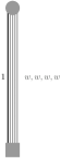
Figure 1: Protograph of ($\alpha$, $d=5$) LDLC. The circle and rectangle nodes represent variable and check nodes, respectively. Black line denotes a edge labeled 1 and gray lines denote edges labeled $w$.

III Spatially Coupled Protograph of LDLC

In this section, we first define ($\alpha,d,L$) SC-LDLC, then ($\alpha,d,L,K$) SC-LDLC will be introduced.

III-A Standard Coupling

We define a ($\alpha,d,L$) SC-LDLC as a dimension $n(L-d+1)$ lattice with an $n(L-d+1)\times nL$ inverse generator matrix $\bm{{\rm H}}_{[L]}$ as described by Eq. (5). The structure of $\bm{{\rm H}}_{[L]}$ is similar to the parity check matrix of tail-biting convolutional codes. In Eq. (5), $\bm{{\rm H}}^{(l)}=\bm{{\rm P}}^{\prime(l)}_{1}+w\sum_{i=2}^{d}\bm{{\rm P}}^{\prime(l)}_{i}$ is an inverse generator matrix of a $n$ dimension ($\alpha,d$) LDLC for $1\leq l\leq L$, and each $\bm{{\rm P}}^{\prime(l)}_{d}$ represents a distinct matrix of the form of (3), for distinct $l$ and $d$.

In this construction, some integers are terminated to 0. The integer vector of the form:

$$\bm{{\rm\tilde{b}}} =\begin{bmatrix}\bm{{\rm b}}\\ \bm{{\rm 0}}_{n(d-1)}\end{bmatrix},$$

is used, so that if $\bm{{\rm x}}\in\Lambda$, then $\bm{{\rm H}}_{[L]}\cdot\bm{{\rm x}}=\bm{{\rm\widetilde{b}}}$. Here, $\bm{{\rm b}}=(b_{1},\ldots,b_{i},\ldots,b_{n(L-d+1)})^{\mathsf{T}}$ is an information integer vector, i.e. $b_{i}\in\mathbb{Z}$. And, $\bm{{\rm 0}}_{n(d-1)}$ is the all zero column vector of length $n(d-1)$. The dimension of the lattice is, therefore, less than the number of elements in $\bm{{\rm x}}$, which is $nL$.

The protograph of ($\alpha$, 5, 18) SC-LDLC is shown in Fig. 2. Reliable messages from white rectangle nodes (null check nodes), i.e., 15, 16, 17, and 18, are gradually propagated. In the protograph, a node corresponds to $n$ variable nodes or $n$ check nodes, and nodes are connected according to an entry in Eq. (5) corresponding to that edge. BP decoding, as well as density evolution, proceeds on the protograph, using $\bm{{\rm H}}_{[L]}$, as with protograph-based LDPC codes [11].

Associated with the lattice is an $nL\times n(L-d+1)$ generator matrix $\bm{{\rm G}}_{[L]}$. The $\bm{{\rm G}}_{[L]}$ has a sub-matrix from column 1 to $n(L-d+1)$ which is an $nL\times nL$ non-singular matrix $\bm{{\rm\tilde{G}}}_{[L]}$. Therefore a lattice point in the dimension $n(L-d+1)$ lattice is generated with

$$\bm{{\rm x}}=\bm{{\rm G}}_{[L]}\bm{{\rm b}}=\bm{{\rm\tilde{G}}}_{[L]}\bm{{\rm\tilde{b}}}.$$ (4)

Dimension ratio is defined as

$$R_{L}=\frac{n(L-d+1)}{nL}=1-\frac{d-1}{L}.$$

The ratio $R_{L}$ converges to 1 with increasing $L$, with gap $O(1/L)$. Therefore, this dimension loss is negligible for sufficiently large $L$.

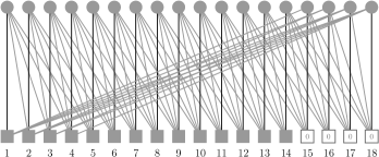
Figure 2: Protograph of ($\alpha$, $d=5$, $L=18$) SC-LDLC. White rectangle nodes are null check nodes corresponding to $\bm{{\rm 0}}_{n(d-1)}$.

$$\bm{{\rm H}}_{[L]} =\begin{bmatrix}\bm{{\rm P}}^{\prime(1)}_{1}&&&&&w\bm{{\rm P}}^{\prime(L-d+2)}_{d}&\cdots&w\bm{{\rm P}}^{\prime(L)}_{2}\\ w\bm{{\rm P}}^{\prime(1)}_{2}&\bm{{\rm P}}^{\prime(2)}_{1}&&&&&\ddots&\vdots\\ \vdots&\vdots&\ddots&&&&&w\bm{{\rm P}}^{\prime(L)}_{d}\\ w\bm{{\rm P}}^{\prime(1)}_{d}&w\bm{{\rm P}}^{\prime(2)}_{d-1}&\ddots&\ddots\\ &\ddots&\ddots&\ddots&\bm{{\rm P}}^{\prime(L-d+1)}_{1}\\ &&\ddots&\ddots&w\bm{{\rm P}}^{\prime(L-d+1)}_{2}&\bm{{\rm P}}^{\prime(L-d+2)}_{1}\\ &&&\ddots&\vdots&\vdots&\ddots\\ &&&&w\bm{{\rm P}}^{\prime(L-d+1)}_{d}&w\bm{{\rm P}}^{\prime(L-d+2)}_{d-1}&\cdots&\bm{{\rm P}}^{\prime(L)}_{1}\end{bmatrix}$$ (5)

III-B Randomized coupling

In order to simplify the evaluation of the noise threshold, we define a ($\alpha,d,L,K$) SC-LDLC in this section. A bipartite graph of a code in the $(\alpha,d,L,K)$ SC-LDLC is constructed as follows. Similar to the ($\alpha,d,L$) SC-LDLC, for each position $l\in\{1,\ldots,L\}$, there are $n$ variable nodes and $n$ check nodes. Each of the $d$ edges of a variable node at position $l$ connects uniformly and independently to a check node at position $\hat{l}\in\{l,\ldots,l+K-1\}$, so that every check node has one edge labeled 1 and $d-1$ edges labeled $w$. Note that $\hat{l}$ is taken modulo $L$ value, if $\hat{l}>L$. In the same way, each of the $d$ edges of a check node at position $l$ connects uniformly and independently to a variable node at position $\check{l}\in\{l-K+1,\ldots,l\}$, so that every variable node has one label 1 edge and $d-1$ label $w$ edges. Note that $\check{l}$ is taken modulo $L$. The variable $K$ is called smoothing parameter, and $K<L$. This approach of randomizing connections is based on that of spatially-coupled LDPC codes [1]. Since $n(K-1)$ check nodes do not have information, the dimension ratio $R_{L}$ of the ($\alpha,d,L,K$) SC-LDLC is as follows:

$$R_{L}=\frac{n(L-K+1)}{nL}=1-\frac{K-1}{L}.$$

Similar to the ($\alpha,d,L$) SC-LDLC, $R_{L}$ converges to 1 as increasing $L$ with gap $O(1/L)$. Therefore we can neglect this dimension loss for sufficient large $L$. We employ ($\alpha,d,L,K$) SC-LDLC for density evolution analysis in the next section.

IV Monte Carlo Density Evolution for
Single Gaussian Decoder of SC-LDLC

In this section we describe a method to find noise thresholds for ($\alpha,d,L,K$) SC-LDLC lattices over the unconstrained-power AWGN channel. For LDPC codes, the BP threshold may be easily evaluated using density evolution which tracks the probability density function of log likelihood ratio messages exchanged between the variable nodes and the check nodes in a bipartite graph [12]. However, density evolution of LDLC lattices is much more complicated. Since messages exchanged in the BP decoder for LDLC lattices are probability density functions, density evolution of the BP decoder must track the probability density function of the message probability density functions. Due to the space limitations, the LDLC lattice BP decoding procedure is omitted; please refer to the paper of Sommer et al. [9] for details.

Here, noise thresholds are found via density evolution, using not true BP, but instead a single-Guassian approximation of the decoder message [13]. In this approximation, the probability density function is approximated using a single-Gaussian message, which is described by just two scalars for each message: a mean and a variance. For conventional LDLC lattices, this approximate method is effective, giving a noise threshold of 0.6 dB [13], the same as the 0.6 dB waterfall region of a dimension $10^{6}$ lattice [9]. Performing density evolution would require a joint distribution in two scalars. While not intractable, this is nonetheless computationally demanding. Instead, Monte Carlo density evolution will be used, as has been done for non-binary low-density parity check codes [14]. We describe Monte Carlo density evolution for the single-Gaussian decoder of the ($\alpha,d,L,K$) SC-LDLC as follows.

Variable (check) node at each position $l$ has two message pools, ${\cal P}^{(l)}_{1}$ and ${\cal P}^{(l)}_{w}$ (${\cal\bar{P}}^{(l)}_{1}$ and ${\cal\bar{P}}^{(l)}_{w}$), which distinguish the edges labeled 1 from those labeled $w$. Both ${\cal P}^{(l)}_{h}$ and ${\cal\bar{P}}^{(l)}_{h}$ have $N_{\textrm{s}}$ messages, i.e.,

$${\cal P}^{(l)}_{h} \!\!\!\!=\!\!\!\!\! \{(m^{(l)}_{h}[1],v^{(l)}_{h}[1]),\ldots,(m^{(l)}_{h}[N_{s}],v^{(l)}_{h}[N_{s}])\}$$

$$\Big{(}{\cal\bar{P}}^{(l)}_{h} \!\!\!\!\!=\!\!\!\!\! \{(\bar{m}^{(l)}_{h}[1],\bar{v}^{(l)}_{h}[1]),\ldots,(\bar{m}^{(l)}_{h}[N_{s}],\bar{v}^{(l)}_{h}[N_{s}])\}\Big{)},$$

for $h\in\{1,w\}$. In the following, the index $[i]$ is omitted. The pair ($m^{(l)}_{h},v^{(l)}_{h}$) $\left((\bar{m}^{(l)}_{h},\bar{v}^{(l)}_{h})\right)$ denotes a mean and a variance of a variable-to-check (check-to-variable) message transmitted from position $l$ along an edge labeled $h$.

IV-1 Initialization

The messages ($m^{(l)}_{h},v^{(l)}_{h}$) $\in{\cal P}^{(l)}_{h}$ for all $l\in\{1,\ldots,L\}$ and $h\in\{1,w\}$ is initialized as follows: The noise variance $\sigma^{2}$ is assigned to $v^{(l)}_{h}$ and the received symbol $\mu$ generated from ${\cal N}(0,\sigma^{2})$ is assigned to $m^{(l)}_{h}$, since the all zero codeword, i.e., $b_{i}=0$ for all $i\in\{1,\ldots,n(L-K+1)\}$, is assumed.

At each half iteration, $N_{s}$ messages in ${\cal P}^{(l)}_{h}$ and ${\cal\bar{P}}^{(l)}_{h}$ are computed alternately for each label $h$ at each position $l$ in the following way.

IV-2 Check node operation

The ($\bar{m}^{(l)}_{h},\bar{v}^{(l)}_{h}$) $\in{\cal\bar{P}}^{(l)}_{h}$ for all $l\in\{1,\ldots,L\}$ and $h\in\{1,w\}$ is computed by

$$\bar{m}^{(l)}_{h}=\frac{1}{h}\sum^{d-1}_{j=1}h_{j}m^{(l_{j})}_{h_{j}},\ \ \ \ \ \bar{v}^{(l)}_{h}=\frac{\sum^{d-1}_{j=1}h_{j}^{2}v^{(l_{j})}_{h_{j}}}{h^{2}},$$

where $l_{j}\in{l-w+1,\ldots,l}\mod{L}$, and $h_{j}\in\{1,w\}$. The $d-1$ messages ($m^{(l_{j})}_{h_{j}},v^{(l_{j})}_{h_{j}}$) are chosen as follows: first the position $l_{j}$ is uniformly selected from ${l-w+1,\ldots,l}\mod{L}$, then ($m^{(l_{j})}_{h_{j}},v^{(l_{j})}_{h_{j}}$) is uniformly picked from the ${\cal P}^{(l_{j})}_{h_{j}}$.

IV-3 Variable node operation

The ($m^{(l)}_{h},v^{(l)}_{h}$) $\in{\cal P}^{(l)}_{h}$ for all $l\in\{1,\ldots,L\}$ and $h\in\{1,w\}$ is computed by

$$(m^{(l)}_{h},v^{(l)}_{h})=Q\bigl{(} (\bar{m}^{(l_{d-1})}_{h_{d-1}},\bar{v}^{(l_{d-1})}_{h_{d-1}}),Q\bigl{(}\cdots,$$

$$Q\bigl{(}(\bar{m}^{(l_{1})}_{h_{1}},\bar{v}^{(l_{1})}_{h_{1}}),(\mu,\sigma^{2})\bigr{)}\cdots\bigr{)}\bigr{)},$$

where $(m,v)=Q\bigl{(}(\bar{m}^{(l_{j})}_{h_{j}},\bar{v}^{(l_{j})}_{h_{j}}),(\hat{m},\hat{v})\bigr{)}$ is recursively computed as follows. First $(\hat{m},\hat{v})$ is initialized by the channel output $(\mu,\sigma^{2})$, then

$$m =\sum_{b\in{\cal B}_{l_{j}}}c^{\prime}(b)m^{\prime}(b),$$

$$v =v^{\prime}+\sum_{b\in{\cal B}_{l_{j}}}c^{\prime}(b)\bigl{(}m^{\prime}(b)\bigr{)}^{2}-\bigl{(}\sum_{b\in{\cal B}_{l_{j}}}c^{\prime}(b)m^{\prime}(b)\bigr{)}^{2},$$

where

$$m^{\prime}(b) =v^{\prime}\bigl{(}\frac{b}{\bar{v}^{(l_{j})}_{h_{j}}h_{j}}-\frac{\bar{m}^{(l_{j})}_{h_{j}}}{\bar{v}^{(l_{j})}_{h_{j}}}+\frac{\hat{m}}{\hat{v}}\bigr{)},$$

$$v^{\prime} =\frac{\bar{v}^{(l_{j})}_{h_{j}}\hat{v}}{\bar{v}^{(l_{j})}_{h_{j}}+\hat{v}},$$

$$c^{\prime}(b) =\frac{1}{Z}\exp\bigl{(}-\frac{(b/h_{j}-\bar{m}^{(l_{j})}_{h_{j}}-\hat{m})^{2}}{2(\bar{v}^{(l_{j})}_{h_{j}}+\hat{v})}\bigr{)},$$

$$Z =\sum_{b\in{\cal B}_{l_{j}}}\exp\bigl{(}-\frac{(b/h_{j}-\bar{m}^{(l_{j})}_{h_{j}}-\hat{m})^{2}}{2(\bar{v}^{(l_{j})}_{h_{j}}+\hat{v})}\bigr{)},$$

$${\cal B}_{l_{j}} =\begin{cases}\mathbb{Z}&l_{j}\in\{1,\ldots,L-K+1\}\\ \{0\}&\text{otherwise}\end{cases}.$$

Similar to the check node operation, the $d-1$ messages $(\bar{m}^{(l_{j})}_{h_{j}},\bar{v}^{(l_{j})}_{h_{j}})$ are chosen as follows: first the position $l_{j}$ is uniformly selected from ${l,\ldots,l+w-1}\mod{L}$, then $(\bar{m}^{(l_{j})}_{h_{j}},\bar{v}^{(l_{j})}_{h_{j}})$ is uniformly picked from the ${\cal\bar{P}}^{(l_{j})}_{h_{j}}$. In this operation, for each ($m^{(l)}_{h},v^{(l)}_{h}$), the $(\mu,\sigma^{2})$ is also re-sampled according to the channel model.

Note that the order of the recursive computation affects the results; the objective here is to minimize the error due to the single-Gaussian approximation. The computations are ordered using the metric

$${\cal M}(j)=\frac{(\bar{m}^{(l_{j})}_{h_{j}}+\hat{m})^{2}}{\bar{v}^{(l_{j})}_{h_{j}}+\hat{v}}.$$

We compute $(\bar{m}^{(l_{j})}_{h_{j}},\bar{v}^{(l_{j})}_{h_{j}})$ beginning with the smallest ${\cal M}(j)$, in order to minimize the single-Gaussian approximation error.

The above procedure repeats until convergence is detected. The mean of the $v^{(l)}_{w}$ of the message in ${\cal P}^{l}_{w}$ for all $l\in\{1,\ldots,L\}$ was used to check convergence. When the mean (over all $N_{s}$ samples at all positions $l$) fell below 0.001, within $I_{\max}$ iterations, then convergence was declared.

V Experimental Results

The noise threshold of conventional ($\alpha,d$) LDLC lattices, measured in distance from capacity, is shown in Fig. 3, for $N_{s}=10^{5}$ samples. The maximum number of iterations is $I_{\max}=50$. The noise threshold improves for increasing $\alpha$ and $d$. In most cases, increasing $\alpha$ above 0.8 had little or no benefit for improving the threshold. Also, the noise threshold gradually improves for increasing $d$, however there appears to be marginal benefit for increasing beyond $d=7$. Since the complexity is proportional to $d$, increasing $d$ beyond this value is not a promising means to improve the threshold. We observe that the smallest gap from the capacity is about 0.5 dB.

Figure 3: Noise threshold, measured in distance from capacity, for various ($\alpha,d$) LDLC. Average variance of messages belonging to nodes labeled $w$ for convergence is $10^{-3}$. The number of samples in pool $N_{s}$ is 100000. The gap from the capacity is about 0.5 dB.

The noise threshold for ($0.8,7,L,2$) SC-LDLC lattices proposed in this paper are shown in Table I, with $I_{\max}=5000$ and $20000$, for various values of the coupling number $L$. We observe that the noise threshold of the (0.8, 7, $L$, 2) SC-LDLC lattice, with sufficiently large $L$ and $I_{\max}$, is very close to the theoretical limit, within 0.22 dB. Note that the gap of the capacity is not a precise value, since the capacity in Eq. (1) assumes lattices defined by full-rank matrices, distinct from SC-LDLC lattices. The threshold approaches the capacity at small $L$, since the dimension ratio is small (the capacity in (1) is not valid in this range). However the capacity loss becomes small, if $L$ becomes large. For example, the dimension ratio is 0.998 at $L=500$. For a practical system which uses shaping, rather than unconstrained power, this is a small penalty. In addition, the noise threshold appears to converge at $L=15$, since the threshold remains 0.22 dB, independently from $L$, for a sufficiently large number of iterations.

The noise threshold for various ($\alpha=0.8,d,L,K$) SC-LDLC lattices are shown in Table II, with $I_{\max}=5000$. The noise threshold does not improve for increasing $d$, this is the same observation as in Fig. 3, however slightly improves for increasing $K$ at the same $R_{L}$. This is because there might be some wiggle [1]. There might be a gap from capacity even if the wiggle vanishes with large $K$.

Fig. 4 shows the trajectory of $v^{(l)}_{w}$ at various node positions as the iterations progress. As expected, the variances from the variable nodes at the start and end position decrease rapidly due to the reliable message from the null check node. This phenomenon is the same as the observation in spatially-coupled LDPC codes over BEC [1].

TABLE I: Noise threshold (in dB) for various ($\alpha=0.8,d=7,L,K=2$) SC-LDLC lattices with $N_{s}=1000$. Note that the threshold approaches the capacity at small $L$, since the dimension ratio is too small (the capacity in (1) is not valid).

$L$	5	8	15	100	300	500
$I_{\max}=5000$	0.00	0.17	0.22	0.22	0.26	0.29
$I_{\max}=20000$	0.00	0.17	0.22	0.22	0.22	0.22

TABLE II: Noise threshold (in dB) for various ($\alpha=0.8,d,L,K$) SC-LDLC with $I_{\max}=5000$ and $N_{s}=1000$. Noise threshold does not improve for increasing $d$, however slightly improves for increasing $K$ at the same $R_{L}$. This is because there might be some wiggle [1].

$d$	7	10	15
$L=100,K=2,R_{L}=0.99$	0.22	0.21	0.22
$L=100,K=5,R_{L}=0.96$	0.21	0.19	0.22
$L=25,K=2,R_{L}=0.96$	0.22	0.21	0.21

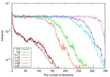
Figure 4: $(\alpha=0.8,d=7,L=31,K=2)$ SC-LDLC, $\sigma^{2}=0.0548905$: Density evolution variance $v^{(l)}_{w}$ at the positions $l=$1, 6, 11, 16, 21, 26, and 31 at the iterations.

VI Conclusion

This paper has described a new LDLC lattice construction, based upon spatial coupling principles. Evaluation was performed using Monte Carlo density evolution using a single-Gaussian approximation of the belief-propagation method. While the conventional lattice construction has a gap of 0.5 dB to capacity, the proposed SC-LDLC construction has a gap of 0.22 dB to capacity, of the unconstrained power channel.

A significant open question remains: how to close up this 0.22 dB gap to capacity? While spatial coupling improves the noise threshold, the ultimate lattice performance can be no better than the ML performance of the lattice itself. This opens the opportunity for new code designs, for example, by more closely considering the edge label values, or allowing for non-uniform degree distributions. On the other hand, we must allow for the possibility that the single-Gaussian approximation introduces errors that limit the threshold under the evaluation method used here.

References

- [1] S. Kudekar, T. Richardson, and R. Urbanke, “Threshold saturation via spatial coupling: Why convolutional LDPC ensembles perform so well over the BEC,” IEEE Transactions on Information Theory, vol. 57, pp. 803–834, February 2011.
- [2] S. Kudekar, C. Méasson, T. J. Richardson, and R. Urbanke, “Threshold saturation on BMS channels via spatial coupling,” in The 6th International Symposium on Turbo Codes and Related Topics, pp. 319–323, September 2010. Brest France.
- [3] S. Kudekar and K. Kasai, “Spatially coupled codes over the multiple access channel,” in Proc. 2011 IEEE Int. Symp. Inf. Theory (ISIT), August 2011. Saint-Petersburg, Russia.
- [4] H. Uchikawa, K. Kasai, and K. Sakaniwa, “Spatially coupled protograph-based LDPC codes for decode-and-forward in erasure relay channel,” in Proc. 2011 IEEE Int. Symp. Inf. Theory (ISIT), August 2011. Saint-Petersburg, Russia.
- [5] S. Kudekar and K. Kasai, “Threshold saturation on channels with memory via spatial coupling,” in Proc. 2011 IEEE Int. Symp. Inf. Theory (ISIT), August 2011. Saint-Petersburg, Russia.
- [6] S. Kudekar and H. D. Pfister, “The effect of spatial coupling on compressive sensing,” in Proc. 48th Annual Allerton Conf. on Commun., Control and Computing, June 2010. Monticello, IL, USA.
- [7] K. Takeuchi, T. Tanaka, and T. Kawabata, “Improvement of BP-based CDMA multiuser detection by spatial coupling,” in Proc. 2011 IEEE Int. Symp. Inf. Theory (ISIT), August 2011. Saint-Petersburg, Russia.
- [8] S. H. Hassani, N. Macris, and R. Urbanke, “Coupled graphical models and their thresholds,” in Proc. 2010 IEEE Information Theory Workshop (ITW), pp. 1–5, September 2010.
- [9] N. Sommer, M. Feder, and O. Shalvi, “Low-density lattice codes,” IEEE Transactions on Information Theory, vol. 54, pp. 1561–1585, April 2008.
- [10] G. Poltyrev, “On coding without restrictions for the AWGN channel,” IEEE Transactions on Information Theory, vol. 40, pp. 409–417, March 1994.
- [11] J. Thorpe, “Low Density Parity Check (LDPC) Codes Constructed from Protographs,” JPL IPN Progress Report 42-154, August 2003.
- [12] T. J. Richardson and R. Urbanke, “The capacity of low-density parity-check codes under message-passing decoding,” IEEE Trans. on Inform. Theory, vol. 47, 2001.
- [13] B. M. Kurkoski, K. Yamaguchi, and K. Kobayashi, “Single-gaussian messages and noise thresholds for decoding low-density lattice codes,” in Proc. 2009 IEEE Int. Symp. Inf. Theory (ISIT), pp. 734–738, July 2009.
- [14] M. Gorgoglione, V. Savin, and D. Declercq, “Split-extended LDPC codes for coded cooperation,” in Proc. Int. Symp. on Inf. Theory and its Applications (ISITA2010), pp. 400–405, 2010.