The charged dust solution of Ruban –
matching to Reissner–Nordström and shell crossings

Abstract

The maximally extended Reissner–Nordström (RN) manifold with $e^{2}<m^{2}$ begs for attaching a material source to it that would preserve the infinite chain of asymptotically flat regions and evolve through the wormhole between the RN singularities. So far, the attempts were discouraging. Here we try one more possible source – a solution found by Ruban in 1972 that is a charged generalisation of an inhomogeneous Kantowski–Sachs-type dust solution. It can be matched to the RN solution, and the matching surface must stay all the time between the two RN event horizons. However, shell crossings do not allow even half a cycle of oscillation between the maximal and the minimal size.

1 Motivation

Avoiding the Big Bang singularity in cosmological models had been a recurring idea in the literature. The hopes for constructing a model without singularity were largely dashed by the singularity theorems of Hawking and Penrose (see Ref. HaEl1973 for a review). They were temporarily revived by the finding of Vickers Vick1973 that in a charged dust model generalising that of Lemaître Lema1933 and Tolman Tolm1934 (LT) the Big Bang can be prevented by the charge distribution, provided that the absolute value of the charge density is, in geometrical units, smaller than the mass density. This finding created another expectation, that a finite ball of charged dust matched to the Reissner Reis1916 – Nordström Nord1918 (RN) solution would be able to collapse and bounce through the wormhole of the maximally extended RN manifold, thereby giving physical meaning to the infinite chain of black holes and asymptotically flat regions. However, this renewed hope was dashed again in 1991 by Ori Ori1991 who proved that, under exactly the same conditions that prevent the Big Bang, shell crossings will inevitably appear and destroy the dust ball before it enters the wormhole. Then, Krasiński and Bolejko KrBo2006 ; KrBo2007 found a gap in Ori’s assumptions and tried to improve upon his result. Namely, Ori assumed that the ratio of the absolute value of the charge density to the mass density (call this ratio $\alpha$) is smaller than 1 everywhere, including the centre of symmetry. Krasiński and Bolejko considered the case when $\alpha\to 1$ at the centre, while being $<1$ everywhere else. The situation turned out to be better, but not definitively. With initial conditions carefully tuned, the charged dust ball could go through the wormhole just once, being destroyed by shell crossings soon after reaching the maximal size in the next asymptotically flat region. Moreover, a direction-dependent singularity necessarily appeared at the centre of the ball at the instant of minimal size. This is not a satisfactory situation, but the best result achieved so far.

In an attempt to find a better model, we now tried to match the Ruban Ruba1972 charged dust solution to the RN metric and see what results. The charged Ruban solution is a generalisation to nonzero charge of the nonstatic dust solution investigated earlier by Ruban Ruba1968 ; Ruba1969 , which in turn is an inhomogeneous generalisation of the Kantowski – Sachs model KaSa1966 . The matching of these two solutions is very easily achieved, with an interesting result. The Ruban solution represents a pulsating charged dust ball whose outer surface must remain forever between the two event horizons of the RN solution. It touches the inner event horizon at its minimal size and the outer horizon at its maximal size. However, a simple investigation shows that shell crossings are inevitable inside the ball and do not allow even a half cycle of an oscillation, appearing between the maximum and minimum size both in the expansion phase and in the collapse phase.

Thus, the field is still open for finding a physical nonstatic source for the RN solution that would proceed through the wormhole. The next thing to do is to find a charged perfect fluid solution of the Einstein – Maxwell equations in which pressure gradients would prevent the formation of shell crossings. This, however, promises to be an extremely difficult task.

In this paper, we first present the RN solution in coordinates adapted to the matching, then the charged Ruban solution as found by the author, then we prove that the matching can be done, and finally we prove that shell crossings in the Ruban solution are inevitable. We also investigate the limit of zero charge of the Ruban – RN configuration. Then the dust source is matched to the Schwarzschild solution across a hypersurface that remains inside the Schwarzschild horizon, only touching it from inside at the moment of maximal expansion. Shell crossings can then be avoided by an appropriate choice of the arbitrary functions in the Ruban model. However, this model has a finite time of existence, being born in a Big Bang that matches to the past Kruskal Krus1960 – Szekeres Szek1960 singularity and crushing into a Big Crunch that matches to the future KS singularity.

We use the signature $(+---)$. We do not assume “units in which $G=c=1$”; whenever these constants are absent, this means they were absorbed into other symbols. For example, our time coordinate will be $t=c\times$ [the physical time], our $M$ will denote $(G/c^{2})\times$ [the mass], etc. The labelling of the coordinates is $(x^{0},x^{1},x^{2},x^{3})=(t,r,\vartheta,\varphi)$.

2 The Reissner–Nordström solution with $e^{2}<m^{2}$ and its maximal extension

The Reissner Reis1916 – Nordström Nord1918 solution in its standard form is

$${\rm d}s^{2}=F{\rm d}t^{2}-(1/F){\rm d}r^{2}-r^{2}\left({\rm d}\vartheta^{2}+\sin^{2}\vartheta{\rm d}\varphi^{2}\right)$$ (2.1)

where

$$F(r)\ {\overset{\rm def}{=}}\ 1-\frac{2m}{r}+\frac{e^{2}}{r^{2}}+\frac{1}{3}\Lambda r^{2}$$ (2.2)

(we include $\Lambda$ for a while). For reference, Fig. 1 (adapted from Ref. PlKr2006 ) shows the Carter – Penrose diagram of the maximal analytic extension of the underlying spacetime for the case $\Lambda=0$ and $e^{2}<m^{2}$, to which we will limit our attention in the main part of this paper. The ragged lines in the diagram are the curvature singularities at $r=0$, the lines marked “inf” are the past and future null infinities, $r_{+}$ are the outer event horizons at

$$r=r_{+}=m+\sqrt{m^{2}-e^{2}},$$ (2.3)

and $r_{-}$ are the inner event horizons at

$$r=r_{-}=m-\sqrt{m^{2}-e^{2}}.$$ (2.4)

These two values of $r$ are zeros of the function $F$ when $\Lambda=0$. Regions I and III are asymptotically flat, regions II and IV are contained between the two horizons. The thin curved lines are those on which $r$ is constant; they are timelike in the asymptotically flat regions where $r>r_{+}$ and inside the inner event horizon where $r<r_{-}$; between the horizons where $r_{-}<r<r_{+}$ they are spacelike.

Figure 1: The conformal diagram of the maximally extended Reissner–Nordström spacetime with $\Lambda=0$ and $e^{2}<m^{2}$. It can either be interpreted as an infinite chain of copies of the segment within the rectangle, or one can identify the upper side of the rectangle with the lower side, obtaining a manifold with closed timelike and null lines. More explanation in the text.

In the following we will be interested in the region between the horizons, where $F<0$, so $r$ in (2.1) becomes the time coordinate and $t$ becomes a spacelike coordinate. It is easy to verify that the lines on which $(t,\vartheta,\varphi)$ are all constant are geodesics.

For later convenience, we rename the coordinates in (2.1) as follows

$$(t,r)=(\rho,R),$$ (2.5)

and then transform the $R$-coordinate in the region $F<0$ to $\tau(R)$ defined by

$$\left(\frac{{\rm d}{R}}{{\rm d}{\tau}}\right)^{2}=-F=-1+\frac{2m}{R}-\frac{e^{2}}{R^{2}}-\frac{1}{3}\Lambda R^{2}.$$ (2.6)

After this, the metric in this region becomes

$${\rm d}s^{2}={\rm d}\tau^{2}-[-F(R(\tau))]{\rm d}\rho^{2}-R^{2}(\tau)\left({\rm d}\vartheta^{2}+\sin^{2}\vartheta{\rm d}\varphi^{2}\right),$$ (2.7)

with $R(\tau)$ being defined by (2.6).

When $\Lambda=0$, eq. (2.6) can be integrated to give the following explicit function $\tau(R)$:

$$\tau-\tau_{0}=\mu\int\frac{{\rm d}R}{\sqrt{-1+{\displaystyle{\frac{2m}{R}}}-{\displaystyle{\frac{e^{2}}{R^{2}}}}}}=-\mu\sqrt{-R^{2}+2mR-e^{2}}+\mu m\arcsin\left(\frac{R-m}{\sqrt{m^{2}-e^{2}}}\right),$$ (2.8)

where $\mu=\pm 1$ and $\tau_{0}$ is an arbitrary constant.

For some purposes it is more convenient to introduce the parameter $\eta$ by $(R-m)/\sqrt{m^{2}-e^{2}}=\sin(\eta-\pi/2)\equiv-\cos\eta$, and then

$$R=m-\sqrt{m^{2}-e^{2}}\cos\eta,\qquad\tau-\widetilde{\tau}_{0}=\mu\left(m\eta-\sqrt{m^{2}-e^{2}}\sin\eta\right),$$ (2.9)

where $\widetilde{\tau}_{0}=\tau_{0}-\mu m\pi/2$. This shows that as $\tau$ increases, $R$ is oscillating between the $r_{-}$ and $r_{+}$ given by (2.3) and (2.4).

3 The charged Ruban solution Ruba1972

To derive this solution, we assume comoving coordinates, spherical symmetry and a charged dust source. For the metric we assume a less general form than spherical symmetry would allow, namely

$${\rm d}s^{2}={\rm e}^{C(t,r)}{\rm d}t^{2}-{\rm e}^{A(t,r)}{\rm d}r^{2}-R^{2}(t)\left[{\rm d}\vartheta^{2}+\sin^{2}(\vartheta){\rm d}\varphi^{2}\right],$$ (3.1)

where $C(t,r)$, $A(t,r)$ and $R(t)$ are functions to be found from the Einstein – Maxwell equations. The limitation of generality is in $R(t)$; in the most general case it would depend on $r$ as well and the field equations would lead to a charged generalisation of the LT model.

Details of the calculation are given in Ref. PlKr2006 . The field equations show that $R,_{t}C,_{r}=0$. With $R,_{t}=0$, we obtain an (electro-) vacuum solution, which is presented in Appendix A – it is a coordinate transform of the well-known Robinson solution Robi1959 . Thus $C,_{r}=0$, which means that the dust is moving on geodesics. A transformation of $t$ can then be used to achieve $C=0$. The other equations imply

$${R,_{t}}^{2}=-1+\frac{2M}{R}-\frac{Q^{2}}{R^{2}}-\frac{1}{3}\Lambda R^{2},$$ (3.2)

where $M$ is a constant of integration, and $Q$ is the electric charge within the sphere of coordinate radius $r$. Since all other quantities in this equation are independent of $r$, it follows that $Q$ must be constant. This implies that the charge density is zero everywhere. Thus, the dust particles must be neutral, they only move in an exterior electric field.

For the other metric function we obtain the following solution:

$${\rm e}^{A/2}=R,_{t}\left[X(r)\int\frac{{\rm d}t}{R{R,_{t}}^{2}}+Y(r)\right],$$ (3.3)

where $X(r)$ and $Y(r)$ are arbitrary functions, and the expression for matter density in energy units is

$$\kappa\epsilon=\frac{2X}{R^{2}{\rm e}^{A/2}}.$$ (3.4)

Equations (3.1) – (3.4) define the charged Ruban solution, first semi-published in 1972 Ruba1972 , and then mentioned in a later paper Ruba1983 . Note that (3.2) is identical to (2.6), so the function $R(t)$ defined by (3.2) will be the same as $R(\tau)$ defined by (2.6). Note also the following:

1. With $X=0$, eq. (3.4) shows that the Ruban solution becomes electro-vacuum; in fact it then becomes the Reissner – Nordström solution expressed in the $(\tau,\rho)$ coordinates defined by (2.5) – (2.6).

2. When $Y=BX$, where $B$ is a constant ($B=0$ being allowed), the $r$-dependence in (3.4) cancels out and by defining a new $r$ by $r^{\prime}=\int X(r){\rm d}r$ we make also the metric independent of $r$. The spacetime then becomes spatially homogeneous with the Kantowski – Sachs symmetry; in fact it is then the generalisation of the Kantowski – Sachs solution to nonzero charge and cosmological constant.

3. The geometry of a 3-space $t=$ const in (3.1) is that of a 3-dimensional cylinder whose sections $r=$ const are spheres, all of the same radius, and the coordinate $r$ measures the position along the generator. The space is inhomogeneous along the $r$-direction, and the electric field has its only component also in the $r$-direction. The radius $R$ of the cylinder evolves with time according to Eq. (3.2).

4. The matter density in this solution, given by (3.4), depends on $r$ and is everywhere positive if $X>0$. Thus, the amount of rest mass contained inside a sphere $r=r_{0}=$ const does depend on the value of $r_{0}$, and is an increasing function of $r$. Nevertheless, as seen from (3.2), the active gravitational mass $M$ that drives the evolution is constant. Ruban Ruba1969 interpreted this property as follows: the gravitational mass defect of any matter added exactly cancels its contribution to the active mass.

4 Matching the Ruban and RN solutions

To match two spacetime regions to each other we have to prove that on the hypersurface $H$ forming the border between them both 4-dimensional metrics induce the same 3-dimensional metric and the same second fundamental form. The formulae we use here are derived in Ref. PlKr2006 .

We will show that the RN metric in the coordinates of (2.6) – (2.7) and the Ruban metric defined by (3.1) – (3.3) with $C=0$ can be matched along any $H$ of constant $\rho=r$. On each such $H$ the 3-metrics will be identical when $\tau$ and $t$ are identified and

$$m=M,\qquad e=Q,$$ (4.1)

since then the $R(\tau)$ of (2.7) and the $R(t)$ of (3.1) will obey the same equation, (2.6) and (3.2) respectively.

The coincidence of the second fundamental forms requires that at $H$ PlKr2006

$$\left.\frac{1}{\cal N}\ \frac{{\rm d}{h_{ij}}}{{\rm d}{r}}\right|_{\rm Ruban}=\left.\frac{1}{\cal N}\ \frac{{\rm d}{h_{ij}}}{{\rm d}{\rho}}\right|_{\rm RN},$$ (4.2)

where $i,j=0,2,3$ and ${\cal N}$ is the $r$-component of the unit normal vector to $H$, thus $\left|g_{rr}\right|{\cal N}^{2}=1$ on each side of $H$. But the relevant components of the Ruban metric do not depend on $r$, and the relevant components of the RN metric do not depend on $\rho$, so (4.2) is fulfilled in a trivial way: it reduces to $0=0$. Note, however, that the matching is possible only in that region of the RN manifold where $F<0$ in (2.1) – (2.2). In the subcase $\Lambda=0$, this is the region between the two event horizons.

Equation (2.9) applies also in the Ruban region, with $m=M$ and $e=Q$. It is independent of $r$, so each constant-$r$ shell evolves by the same law. This means that all shells, including the outer surface of the Ruban region, oscillate between $R=r_{-}$ and $R=r_{+}$, where $r_{-}$ and $r_{+}$ are given by (2.3) – (2.4). If the solution could be continued to infinite values of $t$, the conformal diagram of the complete manifold would look as in Fig. 2. However, shell crossings make the completion of even half a cycle of oscillations impossible, see next section.

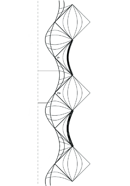
Figure 2: The maximally extended Reissner–Nordström spacetime with a hypothetical charged matter source matched to it. The extent of the source in this diagram is unknown, even if it is the charged Ruban solution – because of the arbitrary functions it contains. This is why the left edge is schematically marked with a dashed line. The two long wavy curves show possible matchings at two different values of the radial coordinate; this coordinate is the $r$ of (5.1) and the $\rho$ of (2.7). Note: these are the curves on which $r$ and $\rho$ are constant. It is $R$ that pulsates between the $r_{-}$ and $r_{+}$ of (2.3) and (2.4), and it changes along these curves. The lines of constant $R$ are the horizontal hyperbola-like arches. If the matter source is the charged Ruban solution, then shell crossings appear within each half-cycle of oscillation. The positions of two of them are schematically marked with thin horizontal straight lines.

5 Shell crossings in the charged Ruban solution are inevitable

For the rest of this article we assume $\Lambda=0$. In this case the Ruban metric is

$${\rm d}s^{2}={\rm d}t^{2}-{\rm e}^{A(t,r)}{\rm d}r^{2}-R^{2}(t)\left({\rm d}\vartheta^{2}+\sin^{2}\vartheta{\rm d}\varphi^{2}\right),$$ (5.1)

where the solution for $R(t)$ can be written as (cf. eq. (2.9)):

$$R=M-\sqrt{M^{2}-Q^{2}}\cos\eta,\qquad t-t_{0}=\mu\left(M\eta-\sqrt{M^{2}-Q^{2}}\sin\eta\right),$$ (5.2)

where $\mu=+1$ in the expansion phase and $\mu=-1$ in the collapse phase. With $\Lambda=0$, the function ${\rm e}^{A/2}$ can be calculated explicitly. For this purpose, we find from (3.2)

$$R,_{t}=\mu\sqrt{-1+\frac{2M}{R}-\frac{Q^{2}}{R^{2}}}.$$ (5.3)

Note that this solution exists only when $Q^{2}<M^{2}$. Now we use this in the integral in (3.3) rewritten as follows

$$\int\frac{{\rm d}t}{R{R,_{t}}^{2}}\equiv\int\frac{{\rm d}R}{R{R,_{t}}^{3}}.$$ (5.4)

Then we obtain

$${\rm e}^{A/2} = X(r)\left[2+Q^{2}\frac{1-M/R}{M^{2}-Q^{2}}-\sqrt{-1+\frac{2M}{R}-\frac{Q^{2}}{R^{2}}}\arcsin\left(\frac{R-M}{\sqrt{M^{2}-Q^{2}}}\right)\right]$$ (5.5)

$$+ \mu Y(r)\sqrt{-1+\frac{2M}{R}-\frac{Q^{2}}{R^{2}}}.$$

A shell crossing is where ${\rm e}^{A/2}=0$, because at such a location two matter shells whose $r$-coordinates differ by ${\rm d}r$ are at a zero distance, as seen from (5.1), and stick together. From (3.4) one sees that at such a location the mass density becomes infinite, so this is a curvature singularity. The question we seek to answer is now: can the functions $X(r)$ and $Y(r)$ in (5.5) be chosen in such a way that ${\rm e}^{A/2}\neq 0$ everywhere.

Unfortunately, the answer given by the formulae above is a definitive “no”, i.e. shell crossings are inevitable. To see this, let us first recall that $R$ changes between the values

$$R_{-}=M-\sqrt{M^{2}-Q^{2}},\qquad{\rm and}\qquad R_{+}=M+\sqrt{M^{2}-Q^{2}}$$ (5.6)

(this is a copy of (2.3) – (2.4) rewritten in the notation for the Ruban model). At both these values the expression under the square root in (5.5) is zero, and in the whole range $0<R_{-}<R<R_{+}$ the function ${\rm e}^{A/2}$ given by (5.5) is continuous. Now, at $R=R_{-}$ we have

$$\left.{\rm e}^{A/2}\right|_{R=R_{-}}=-X(r)\frac{R_{-}}{\sqrt{M^{2}-Q^{2}}},$$ (5.7)

while at $R=R_{+}$ we have

$$\left.{\rm e}^{A/2}\right|_{R=R_{+}}=X(r)\frac{R_{+}}{\sqrt{M^{2}-Q^{2}}}.$$ (5.8)

Thus, whatever the sign of $X(r)$, the signs of ${\rm e}^{A/2}$ at the ends of the range $\left[R_{-},R_{+}\right]$ are opposite, i.e. ${\rm e}^{A/2}=0$ for some value of $R$ within this range. This is a shell crossing. Note that it appears every time when $R$ traverses this range, which means that the shell crossings will not allow $R$ to go through even half a cycle of oscillation.

The geometrical nature of this shell crossing is different than in the LT and Szekeres models Szek1975a ; Szek1975b , where they have been investigated quite thoroughly HeLa1985 ; HeKr2002 ; HeKr2008 . In the LT and Szekeres models, the spheres that collide are one within the other. At a shell crossing, the smaller sphere catches up with the larger one during expansion (or vice versa during collapse). In the Ruban model, the spheres are surfaces of constant $r$ in the 3-dimensional cylinder $t=$ constant, and they move up and down along the generators as the cylinder expands or collapses. It turns out they will collide before the cylinder manages to proceed all the way from the minimal radius to maximal, or from maximal to minimal. One more property of such a shell crossing is noteworthy: its locus does not depend on $r$, which means that all the spheres with different values of $r$ collide at the same moment.

Kantowski and Sachs KaSa1966 noted the possible occurrence of this singularity in the subcase $Q=Y(r)=0$ of the Ruban model, where they said “The singularities for the closed models are of two kinds. (…) In one kind of a singularity the cylinder squashes to a disk, in the other it contracts to a line.” What we called shell crossing here is the “squashing to a disk”.

The shell crossings could possibly be prevented by pressure with a nonzero gradient in the $r$-direction, but such exact solutions are not yet known. Then, assuming that the pressure and its gradient would be zero at the surface of the charged fluid ball, its surface would follow a timelike geodesic in the RN spacetime, and the conformal diagram could really look like Fig. 2.

6 Absence of shell crossings in the Ruban solution with zero charge

When $Q=0$, the charged Ruban solution goes over into the Datt – Ruban neutral dust solution Datt1938 ; Ruba1969 ; PlKr2006 . Then from (2.9), adapted to the notation for the Ruban solution, we obtain

$$R=M(1-\cos\eta),\qquad t-t_{0}=\mu M(\eta-\sin\eta).$$ (6.1)

This shows that now $R$ starts from 0 at $t=t_{0}$, then increases to $2M$ at $t=t_{0}+\mu M\pi$, and decreases to 0 again at $t=t_{0}+2\mu M\pi$. At $R=0$ the model has a Big Bang/Crunch type singularity. Equation (5.5) simplifies to

$${\rm e}^{A/2}=\sqrt{-1+\frac{2M}{R}}\left\{X(r)\left[\frac{2}{\sqrt{-1+\frac{2M}{R}}}-\arcsin\left(\frac{R}{M}-1\right)\right]+\mu Y(r)\right\}\ {\overset{\rm def}{=}}\ \sqrt{-1+\frac{2M}{R}}{\cal F}(t,r).$$ (6.2)

Now the spacetime is singular at $R=0$, so the model exists only for the finite time $T=2\pi M$ between the Big Bang and Big Crunch, but, unlike in the charged case, the functions $X(r)$ and $Y(r)$ can be chosen so that within this interval there are no shell crossings. We show below that, with an appropriate choice, ${\cal F}>0$ during the whole evolution.

Namely, with $R=0$ at the start of the expansion phase, where $\mu=+1$, we have

$$\left.{\cal F}\right|_{R=0}=X\frac{\pi}{2}+Y.$$ (6.3)

Thus, $X>0$ and $Y>0$ will guarantee that $\left.{\cal F}\right|_{R=0,\mu=+1}>0$. We also have

$$\frac{{\rm d}{\cal F}}{{\rm d}{R}}=\frac{X}{R\left(\frac{2M}{R}-1\right)^{3/2}},$$ (6.4)

which will be positive for all $0\leq R<2M$ if $X>0$, becoming $+\infty$ as $R\to 2M$. Since also ${\cal F}\to+\infty$ as $R\to 2M$, the switch from expansion to collapse, i.e. from $\mu=+1$ to $\mu=-1$, will keep ${\cal F}$ positive at the beginning of collapse. So we only have to guarantee that ${\cal F}>0$ at the end of the collapse phase, when $R\to 0$ again. This will be the case when

$$\left.{\cal F}\right|_{R=0,\mu=-1}=X\frac{\pi}{2}-Y>0.$$ (6.5)

Consequently, both (6.3) and (6.5) will be positive during the whole cycle when

$$0<Y<X\frac{\pi}{2}$$ (6.6)

at all values of $r$. The fact that the shell crossings become absent when $Q=0$ shows that the limiting transition $Q\to 0$ is discontinuous; just as it was in the RN $\to$ Schwarzschild transition.

The neutral Ruban solution can be matched to the Schwarzschild solution, as shown by Ruban himself Ruba1969 . The matching hypersurface stays within the Schwarzschild radius except at $R=2M$, when it touches the horizon from inside. However, this configuration has a finite time of existence, just as the Kruskal Krus1960 – Szekeres Szek1960 manifold between its two singularities.

7 Summary

We investigated the charged Ruban solution Ruba1972 as a possible matter source for the maximally extended Reissner – Nordström solution with $e^{2}<m^{2}$. The matching of these two solutions is easily achieved. The hypersurface that forms the boundary between the Ruban and RN regions stays all the time between the two RN event horizons, touching the inner one at its minimal radius and the outer one at maximal radius. However, shell crossings make the completion of even half a cycle of such an oscillation impossible; they appear between each $[r_{-},r_{+}]$ and each $[r_{+},r_{-}]$ pair.

Shell crossings can be avoided in the limit of zero charge, when the arbitrary functions in the Ruban solution obey a simple inequality. Then the Ruban solution can be matched to the Schwarzschild solution inside the event horizon, but the model has a finite time of existence.

The problem of finding a matter source to the maximally extended RN solution thus still remains open, with one more possibility being now elliminated.

Appendix A The limiting case $Q^{2}=M^{2},\Lambda=0$

As stated in the footnote below (5.3), this leads to the static solution $R=M=|Q|$. This limit is not a subcase of (3.3), and the Einstein – Maxwell equations have to be solved anew. With $R,_{t}=0$ they lead to the electro-vacuum solution, in which

$${\rm e}^{A/2}=\alpha(r)\cos(t/M)+\beta(r)\sin(t/M),$$ (A.1)

where $\alpha(r)$ and $\beta(r)$ are arbitrary functions, and the metric is

$${\rm d}s^{2}={\rm d}t^{2}-{\rm e}^{A}{\rm d}r^{2}-M^{2}\left({\rm d}\vartheta^{2}+\sin^{2}\vartheta{\rm d}\varphi^{2}\right)$$ (A.2)

(we recall that $M=|Q|$, where $Q$ is the electric charge). This should be compared to the Nariai solution Nari1950 in the form found by Krasiński and Plebański KrPl1980 :

$${\rm d}s^{2}=[a(t)\cos(\rho/\ell)+b(t)\sin(\rho/\ell)]^{2}{\rm d}t^{2}-{\rm d}\rho^{2}-\ell^{2}\left({\rm d}\vartheta^{2}+\sin^{2}\vartheta{\rm d}\varphi^{2}\right),$$ (A.3)

where $\ell$ is an arbitrary nonzero constant. This is a vacuum solution with the cosmological constant $\Lambda=1/\ell^{2}$. Equation (A.3) is related to (A.1) – (A.2) by the interchange of $t$ and $r$, and has the same geometrical structure – it is a Cartesian product of two surfaces of constant curvature.

In fact, (A.1) – (A.2) is a coordinate transform of the Robinson solution Robi1959 . Namely, by a rather complicated sequence of coordinate transformations, strictly analogous to those used in Ref. KrPl1980 for the Nariai solution, (A.1) – (A.2) may be transformed to

$${\rm d}s^{2}=\frac{\ell^{2}}{{r^{\prime}}^{2}}\left[{\rm d}t^{2}-{\rm d}{r^{\prime}}^{2}-{r^{\prime}}^{2}\left({\rm d}\vartheta^{2}+\sin^{2}\vartheta{\rm d}\varphi^{2}\right)\right],$$ (A.4)

which is identical with one of Robinson’s formulae, with Robinson’s $\lambda=1/\ell$.

Acknowledgement: The research of AK was supported by the Polish Ministry of Education and Science grant no N N202 104 838. While the paper was being prepared, GG was a summer intern at the N. Copernicus Astronomical Center in Warsaw.

References

- (1) S. W. Hawking and G. F. R. Ellis, The Large-scale Structure of Spaceetime. Cambridge University Press (1973).
- (2) P. A. Vickers, Ann. Inst. Poincaré A18, 137 (1973).
- (3) G. Lemaître, Ann. Soc. Sci. Bruxelles A53, 51 (1933); English translation, with historical comments: Gen. Rel. Grav. 29, 637 (1997).
- (4) R.C. Tolman, Proc. Nat. Acad. Sci. USA 20, 169 (1933); reprinted, with historical comments: Gen. Rel. Grav. 29, 931 (1997).
- (5) M. A. Markov and V. P. Frolov, Teor. Mat. Fiz. 3, 3 (1970); English translation: Theor. Math. Phys. 3, 301 (1970).
- (6) H. Reissner, Ann. Physik 50, 106 (1916).
- (7) G. Nordström, Koninklijke Nederlandsche Akademie van Wetenschappen Proceedings 20, 1238 (1918).
- (8) J. C. Graves and D. R. Brill, Phys. Rev. 120, 1507 (1960).
- (9) B. Carter, Phys. Lett. 21, 423 (1966).
- (10) B. Carter, in: Black Holes – les astres occlus. Edited by C. de Witt and B. S. de Witt. Gordon and Breach, New York, London, Paris, p. 61 (1973); reprinted, with corrections and editorial comments, in Gen. Rel. Grav. 41, 2867 (2009).
- (11) J. Plebański and A. Krasiński, An Introduction to General Relativity and Cosmology, Cambridge University Press, Cambridge 2006.
- (12) A. Ori, Phys. Rev. D44, 2278 (1991).
- (13) A. Krasiński and K. Bolejko, Phys. Rev. D73, 124033 (2006) + erratum Phys. Rev. D75, 069904 (2007). Fully corrected text available from gr-qc 0602090.
- (14) A. Krasiński and K. Bolejko, Phys. Rev. D76, 124013 (2007).
- (15) V. A. Ruban, in: Tezisy dokladov 3-y Sovetskoy Gravitatsyonnoy Konferentsii [Theses of Lectures of the 3rd Soviet Conference on Gravitation]. Izdatel’stvo Erevanskogo Universiteta, Erevan, pp. 348 – 351 (1972). [Available in Russian only]
- (16) V. A. Ruban, Pis’ma v Red. ZhETF 8, 669 (1968); English translation: Sov. Phys. JETP Lett. 8, 414 (1968); reprinted, with historical comments: Gen. Rel. Grav. 33, 363 (2001).
- (17) V. A. Ruban, Zh. Eksper. Teor. Fiz. 56, 1914 (1969); English translation: Sov. Phys. JETP 29, 1027 (1969); reprinted, with historical comments: Gen. Rel. Grav. 33, 375 (2001).
- (18) R. Kantowski and R. K. Sachs, J. Math. Phys. 7, 443 (1966).
- (19) B. Datt, Z. Physik 108, 314 (1938); English translation, with historical comments: Gen. Rel. Grav. 31, 1615 (1999).
- (20) I. Robinson, Bull. Acad. Polon. Sci., Ser. Mat. Fis. Astr. 7, 351 (1959).
- (21) M. Kruskal, Phys. Rev. 119, 1743 (1960).
- (22) G. Szekeres, Publicationes Mathematicae Debrecen 7, 285 (1960); reprinted, with historical comments: Gen. Rel. Grav. 34, 1995 (2002).
- (23) V. A. Ruban, Zh. Eksper. Teor. Fiz. 85, 801 (1983); English translation: Sov. Phys. JETP 58, 463 (1983).
- (24) P. Szekeres, Comm. Math. Phys. 41, 55 (1975).
- (25) P. Szekeres, Phys. Rev. D 12, 2941 (1975).
- (26) C. Hellaby and K. Lake, Astrophys. J. 290, 381 (1985) + erratum Astrophys. J. 300, 461 (1985).
- (27) C. Hellaby and A. Krasinski Phys. Rev. D 66, 084011, (2002).
- (28) C. Hellaby and A. Krasiński, Phys. Rev. D77, 023529 (2008).
- (29) H. Nariai, Scientific Reports of the Tôhoku University 34, 160 (1950); 35, 46 (1951); both papers reprinted, with historical comments, in Gen. Rel. Grav. 31, 951 (1999).
- (30) A. Krasiński and J. Plebański, Rep. Math. Phys. 17, 217 (1980).