A new multivariate measurement error model with zero-inflated dietary data, and its application to dietary assessment

Abstract

In the United States the preferred method of obtaining dietary intake data is the 24-hour dietary recall, yet the measure of most interest is usual or long-term average daily intake, which is impossible to measure. Thus, usual dietary intake is assessed with considerable measurement error. Also, diet represents numerous foods, nutrients and other components, each of which have distinctive attributes. Sometimes, it is useful to examine intake of these components separately, but increasingly nutritionists are interested in exploring them collectively to capture overall dietary patterns. Consumption of these components varies widely: some are consumed daily by almost everyone on every day, while others are episodically consumed so that 24-hour recall data are zero-inflated. In addition, they are often correlated with each other. Finally, it is often preferable to analyze the amount of a dietary component relative to the amount of energy (calories) in a diet because dietary recommendations often vary with energy level. The quest to understand overall dietary patterns of usual intake has to this point reached a standstill. There are no statistical methods or models available to model such complex multivariate data with its measurement error and zero inflation. This paper proposes the first such model, and it proposes the first workable solution to fit such a model. After describing the model, we use survey-weighted MCMC computations to fit the model, with uncertainty estimation coming from balanced repeated replication. The methodology is illustrated through an application to estimating the population distribution of the Healthy Eating Index-2005 (HEI-2005), a multi-component dietary quality index involving ratios of interrelated dietary components to energy, among children aged 2–8 in the United States. We pose a number of interesting questions about the HEI-2005 and provide answers that were not previously within the realm of possibility, and we indicate ways that our approach can be used to answer other questions of importance to nutritional science and public health.

TITL1Supported by National Science Foundation Instrumentation Grant number 0922866.

, , , , , , , , and aut1Supported by a Grant from the National Cancer Institute (CA57030). aut2This paper forms part of Zhang’s Ph.D. dissertation at Texas A&M University.

1 Introduction.

This paper presents statistical models and methodology to overcome a major stumbling block in the field of dietary assessment. More nutritional background is provided in Section 2: a summary of the key conceptual issues follows:

• Nutritional surveys conducted in the United States typically use 24-hour (24 h) dietary recalls to obtain intake data, that is, an assessment of what was consumed in the past 24 hours.

• Because dietary recommendations are intended to be met over time, nutritionists are interested in “usual” or long-term average daily intake.

• Dietary intake is thus assessed with considerable measurement error.

• Consumption patterns of dietary components vary widely; some are consumed daily by almost everyone, while others are episodically consumed so that 24-hour recall data are zero-inflated. Further, these components are correlated with one another.

• Nutritionists are interested in dietary components collectively to capture patterns of usual dietary intake, and thus need multivariate models for usual intake.

• These multivariate models for usual intakes, taking into account episodically consumed foods, do not exist, nor do methods exist for fitting them.

One way to capture dietary patterns is by scores, although our work is not limited to scores. The Healthy Eating Index-2005 (HEI-2005), described in detail in Section 2, is a scoring system based on a priori knowledge of dietary recommendations, and is on a scale of 0–100. Ideally, it consists of the usual intake of 6 episodically consumed and thus 24 h-zero inflated foods, 6 daily-consumed dietary components, adjusts these for energy (caloric) intake, and gives a score to each component. The total score is the sum of the individual component scores. Higher scores indicate greater compliance with dietary guidelines and, therefore, a healthier diet. Here are a few questions that nutritionists have not been able to answer, and that our approach can address:

• What is the distribution of the HEI-2005 total score, and what % of Americans are eating a healthier diet defined, for example, by a total score exceeding 80?

• What is the correlation between the individual score on each dietary component and the scores of all other dietary components?

• Among those whose total HEI-2005 score is $>$50 or $\leq$50, what is the distribution of usual intake of whole grains, whole fruits, dark green and orange vegetables and legumes (DOL) and calories from solid fats, alcoholic beverages and added sugars (SoFAAS)?

• What % of Americans exceed the median score on all 12 HEI-2005 components?

In this paper, to answer public health questions such as these that can have policy implications, we build a novel multivariate measurement error model for estimating the distributions of usual intakes, one that accounts for measurement error and zero-inflation, and has a special structure associated with the zero-inflation. Previous attempts to fit even simple versions of this model, using nonlinear mixed effects software, failed because of the complexity and dimensionality of the model. We use survey-weighted Monte Carlo computations to fit the model with uncertainty estimation coming from balanced repeated replication. The methodology is illustrated using the HEI-2005 to assess the diets of children aged 2–8 in the United States. This work represents the first analysis of joint distributions of usual intakes for multiple food groups and nutrients.

The paper is outlined as follows. In Section 2 we give the background for the data we observe. In particular, we provide more information about the HEI-2005. Section 3 describes our model which is a highly nonlinear, zero-inflated, repeated measures model with multiple latent variables. The model also has a patterned covariance matrix with structural zeros and ones. We derive a parameterization that allows estimated covariance matrices to be actual covariance matrices. We also define technically what we mean by usual intake, and illustrate the use of simulation methods used to answer the questions posed above, as well as many others.

Section 4 describes our estimation procedure. Previous attempts using nonlinear mixed effects models to estimate the distribution of episodically consumed food groups [Tooze et al. (2006); Kipnis et al. (2009)] do not work here because of the high dimensionality of the problem. We instead develop a Monte Carlo strategy based on the idea of Gibbs sampling; although because of sampling weights, we treat the method as a frequentist (non-Bayesian) one. This section describes some of the basics of the methodology; the full technical details of implementation are given in the Appendix.

Section 5 describes the analysis of the HEI-2005 components using the 2001–2004 National Health and Nutrition Examination Survey (NHANES) for children ages 2–8. Important contextual points arise because of the nature of the data. For example, if whole grains are consumed, then necessarily total grains are consumed with probability one, a restriction that a naive use of our model cannot handle. We develop a simple novel device to uncouple consumption variables that are tightly linked in this way. Finally, in this section we provide the first answers to the four questions we have posed. In Section 6 we discuss various additional aspects of the problem and the data analysis. Concluding remarks and a policy application are given in Section 7.

There are a number of general reviews of the measurement error field [Fuller (1987); Gustafson (2004); Carroll et al. (2006); Buonaccorsi (2010)]. Recent papers that focus on estimating the density function of a univariate continuous random variable subject to measurement error include Delaigle (2008), Delaigle and Hall (2008, 2011), Delaigle and Meister (2008), Delaigle, Hall and Meister (2008), Staudenmayer, Ruppert and Buonaccorsi (2008) and Wand (1998). The field of measurement error in regression continues to expand rapidly, with some recent contributions including Küchenhoff, Mwalili and Lesaffre (2006), Guolo (2008), Liang et al. (2008), Messer and Natarajan (2008) and Natarajan (2009). There is also a large statistical literature on measurement error as it relates to public health nutrition: some recent papers relevant to our work include Carriquiry (1999, 2003), Ferrari et al. (2009), Fraser and Shavlik (2004), Kott et al. (2009), Nusser et al. (1996), Nusser, Fuller and Guenther (1997), Prentice (1996, 2003), Tooze, Grunwald and Jones (2002) and Tooze et al. (2006).

2 Data and the HEI-2005 scores.

Here we give more detail about the nutrition context that motivates this work.

Table 1: Description of the HEI-2005 scoring system. Except for saturated fat and SoFAAS, density is obtained by multiplying usual intake by 1000 and dividing by usual intake of kilocalories

Component	Units	HEI-2005 score calculation
Total fruit	cups	$\min{(5,5\times(\mathrm{density}/0.8))}$
Whole fruit	cups	$\min{(5,5\times(\mathrm{density}/0.4))}$
Total vegetables	cups	$\min{(5,5\times(\mathrm{density}/1.1))}$
DOL	cups	$\min{(5,5\times(\mathrm{density}/0.4))}$
Total grains	ounces	$\min{(5,5\times(\mathrm{density}/3))}$
Whole grains	ounces	$\min{(5,5\times(\mathrm{density}/1.5))}$
Milk	cups	$\min{(10,10\times(\mathrm{density}/1.3))}$
Meat and beans	ounces	$\min{(10,10\times(\mathrm{density}/2.5))}$
Oil	grams	$\min{(10,10\times(\mathrm{density}/12))}$
Saturated fat	% of	if $\mathrm{density}\geq 15$ score${}={}$0
	energy	else if $\mathrm{density}\leq 7$ score${}={}$10
		else if $\mathrm{density}>10$ $\mbox{score}=8-(8\times(\mathrm{density}-10)/5)$
		else, $\mbox{score}=10-(2\times(\mathrm{density}-7)/3)$
Sodium	milligrams	if $\mathrm{density}\geq 2000$ score${}={}$0
		else if $\mathrm{density}\leq 700$ score${}={}$10
		else if $\mathrm{density}\geq 1100$
		$\mbox{score}=8-\{8\times(\mathrm{density}-1100)/(2000-1100)\}$
		else $\mbox{score}=10-\{2\times(\mathrm{density}-700)/(1100-700)\}$
SoFAAS	% of	if $\mathrm{density}\geq 50$ score${}={}$0
	energy	else if $\mathrm{density}\leq 20$ score${}={}$20
		else $\mbox{score}=20-\{20\times(\mathrm{density}-20)/(50-20)\}$

[]For saturated fat, density is $9\times 100$ usual saturated fat (grams) divided by usual calories, that is, the percentage of usual calories coming from usual saturated fat intake. For SoFAAS, the density is the percentage of usual intake that comes from usual intake of calories, that is, the division of usual intake of SoFAAS by usual intake of calories. Here, “DOL” is dark green and orange vegetables and legumes. Also, “SoFAAS” is calories from solid fats, alcoholic beverages and added sugars. The total HEI-2005 score is the sum of the individual component scores.

In surveys conducted in the United States, the preferred method of obtaining intake data is the 24-hour dietary recall because it limits respondent burden and facilitates accurate reporting; yet the measure of greatest interest is “usual” or long-term average daily intake. Thus, dietary intake is assessed with considerable measurement error. Also, diets are comprised of numerous foods, nutrients and other components, each of which may have distinctive attributes and effects on nutritional health. Sometimes, it is useful to examine intake of these components separately, but increasingly nutritionists are interested in exploring them collectively to capture patterns of dietary intake. Consumption patterns of these components vary widely; some are consumed daily by almost everyone, while others are episodically consumed so that 24-hour recall data are zero-inflated. In addition, these various components are often correlated with one another. Finally, it is often preferable to analyze the amount of a dietary component relative to the amount of energy (calories) in a diet because dietary recommendations often vary with energy level, and this approach provides a way of standardizing dietary assessments.

One of the US Department of Agriculture’s (USDA’s) strategic objectives is “to promote healthy diets” and it has developed an associated performance measure, the Healthy Eating Index-2005 (HEI-2005, http:// www.cnpp.usda.gov/HealthyEatingIndex.htm). The HEI-2005 is based on the key recommendations of the 2005 Dietary Guidelines for Americans (http://www.health.gov/dietaryguidelines/dga2005/document/default.htm). The index includes ratios of interrelated dietary components to energy. The HEI-2005 comprises 12 distinct component scores and a total summary score. See Table 1 for a list of these components and the standards for scoring, and see Guenther, Reedy and Krebs-Smith (2008) for details. Intakes of each food or nutrient, represented by one of the 12 components, are expressed as a ratio to energy intake, assessed, and ascribed a score.

The HEI-2005 is used to evaluate the diets of Americans to assess compliance with the 2005 Dietary Guidelines, yet use of the HEI-2005 is limited by the challenges described above. Until recently, there have been no solutions to these challenges, so published evaluations have been limited to analyses of mean scores for the population and various subgroups. Freedman et al. (2010) have described a method of estimating the population distribution of a single component of HEI-2005, and the prevalence of high or low scores on that component; but there has been to date no satisfactory way to determine the prevalence of high or low total HEI-2005 scores, considering all of its interrelated components simultaneously. In addition, answers to the complex questions posed in the Introduction remain unavailable. This paper aims to provide a means to do these crucial evaluations.

The 12 HEI-2005 components represent 6 episodically consumed food groups (total fruit, whole fruit, total vegetables, dark green and orange vegetables and legumes or DOL, whole grains and milk), 3 daily-consumed food groups (total grains, meat and beans and oils) and 3 other daily-consumed dietary components (saturated fat; sodium; and calories from solid fats, alcoholic beverages and added sugars, or SoFAAS). The classification of food groups as “episodically” and “daily” consumed is based on the number of individuals who report them on 24 h recalls. If there are only a few zeros for a component, we treat that as a daily-consumed food, and replace all zeros with $1/2$ the minimum value of the nonzeros for that food. However, the crucial statistical aspect of the data is that six of the food groups are zero-inflated. The percentages of reported nonconsumption of total fruit, whole fruit, whole grains, total vegetables, DOL and milk on any single day are 17%, 40%, 42%, 3%, 50% and 12%, respectively.

We are interested in the usual intake of foods for children aged 2–8. The data available to us, described in more detail in Section 5, came from the National Health and Nutrition Examination Survey, 2001–2004 (NHANES). The data used here consisted of $n=2\mbox{,}638$ children, each of whom had a survey weight $w_{i}$ for $i=1,\ldots,n$. In addition, one or two 24 h dietary recalls were available for each individual. Along with the dietary variables, there are covariates such as age, gender, ethnicity, family income and dummy variables that indicate a weekday or a weekend day, and whether the recall was the first or second reported for that individual.

Using the 24 h recall data reported, for each of the episodically consumed food groups, two variables are defined: (a) whether a food from that group was consumed; and (b) the amount of the food that was reported on the 24 h recall. For the 6 daily-consumed food groups and nutrients, only one variable indicating the consumption amount is defined. In addition, the amount of energy that is calculated from the 24 h recall is of interest. The number of dietary variables for each 24 h recall is thus $12+6+1=19$. The observed data are $Y_{ijk}$ for the $i$th person, the $j$th variable and the $k$th replicate, $j=1,\ldots,19$ and $k=1,\ldots,m_{i}$. In the data set, at most two 24 h recalls were observed, so that $m_{i}\leq 2$. Set $\widetilde{Y}_{ik}=(Y_{i1k},\ldots,Y_{i,19,k})^{\mathrm{T}}$, where

• $Y_{i,2\ell-1,k}=\mbox{Indicator}$ of whether dietary component #$\ell$ is consumed, with $\ell=1,2,3,4,5,6$.

• $Y_{i,2\ell,k}=\mbox{Amount}$ of food #$\ell$ consumed. This equals zero, of course, if none of food #$\ell$ is consumed, with $\ell=1,2,3,4,5,6$.

• $Y_{i,\ell+6,k}=\mbox{Amount}$ of nonepisodically consumed food or nutrient #$\ell$, with $\ell=7,8,9,10,11,12$.

• $Y_{i,19,k}=\mbox{Amount}$ of energy consumed as reported by the 24 h recall.

3 Model and methods.

3.1 Basic model description.

Our model is a generalization of work by Tooze et al. (2006) and Kipnis et al. (2009) for a single food and Kipnis et al. (2011) and Zhang et al. (2011) for a single food and nutrient. Observed data will be denoted as $Y$, and covariates in the model will be denoted as $X$. As is usual in measurement error problems, there will also be latent variables, which will be denoted by $W$.

We use a probit threshold model. Each of the 6 episodically consumed foods will have 2 sets of latent variables, one for consumption and one for amount, while the 6 daily-consumed foods and nutrients as well as energy will have 1 set of latent variables, for a total of 19. The latent random variables are $\varepsilon_{ijk}$ and $U_{ij}$, where $(U_{i1},\ldots,U_{i,19})=\operatorname{Normal}(0,\Sigma_{u})$ and $(\varepsilon_{i1k},\ldots,\varepsilon_{i,19,k})=\operatorname{Normal}(0,\Sigma_{\varepsilon})$ are mutually independent. In this model, food $\ell=1,\ldots,6$ being consumed on day $k$ is equivalent to observing the binary $Y_{i,2\ell-1,k}$, where

$$Y_{i,2\ell-1,k}=1$$

(1)

$$\qquad\iff\quad W_{i,2\ell-1,k}=X_{i,2\ell-1,k}^{\mathrm{T}}\beta_{2\ell-1}+U_{i,2\ell-1}+\varepsilon_{i,2\ell-1,k}>0.$$

If the food is consumed, we model the amount reported $Y_{i,2\ell,k}$ as

$$[g_{\mathrm{tr}}(Y_{i,2\ell,k},\lambda_{\ell})|Y_{i,2\ell-1,k}=1] = W_{i,2\ell,k}$$

$$= X_{i,2\ell,k}^{\mathrm{T}}\beta_{2\ell}+U_{i,2\ell}+\varepsilon_{i,2\ell,k},$$

where $g_{\mathrm{tr}}(y,\lambda)=\sqrt{2}\{g(y,\lambda)-\mu(\lambda)\}/\sigma(\lambda)$, $g(y,\lambda)$ is the usual Box-Cox transformation with transformation parameter $\lambda$, and $\{\mu(\lambda),\sigma(\lambda)\}$ are the sample mean and standard deviation of $g(y,\lambda)$, computed from the nonzero food data. This standardization is simply a convenient device to improve the numerical performance of our algorithm without affecting the conclusions of our analysis.

The reported consumption of daily consumed foods or nutrients $\ell=\break 7,\ldots,12$ is modeled as

$$g_{\mathrm{tr}}(Y_{i,\ell+6,k},\lambda_{\ell}) = W_{i,\ell+6,k}=X_{i,\ell+6,k}^{\mathrm{T}}\beta_{\ell+6}+U_{i,\ell+6}+\varepsilon_{i,\ell+6,k}.$$ (3)

Finally, energy is modeled as

$$g_{\mathrm{tr}}(Y_{i,19,k},\lambda_{13}) = W_{i,19,k}=X_{i,19,k}^{\mathrm{T}}\beta_{19}+U_{i,19}+\varepsilon_{i,19,k}.$$ (4)

As seen in (3.1)–(4), different transformations $(\lambda_{1},\ldots,\lambda_{13})$ are allowed to be used for the different types of dietary components; see Section .15.

In summary, there are latent variables $\widetilde{W}_{ik}=(W_{i1k},\ldots,W_{i,19,k})^{\mathrm{T}}$, latent random effects $\widetilde{U}_{i}=(U_{i1},\ldots,U_{i,19})^{\mathrm{T}}$, fixed effects $(\beta_{1},\ldots,\beta_{19})$, and design matrices $(X_{i1k},\ldots,X_{i,19,k})$. Define $\widetilde{\varepsilon}_{ik}=(\varepsilon_{i1k},\ldots,\varepsilon_{i,19,k})^{\mathrm{T}}$. The latent variable model is

$$W_{ijk} = X_{ijk}^{\mathrm{T}}\beta_{j}+U_{ij}+\varepsilon_{ijk},$$ (5)

where $\widetilde{U}_{i}=\operatorname{Normal}(0,\Sigma_{u})$ and $\widetilde{\varepsilon}_{ik}=\operatorname{Normal}(0,\Sigma_{\varepsilon})$ are mutually independent.

3.2 Restriction on the covariance matrix.

Two necessary restrictions are set on $\Sigma_{\varepsilon}$. First, following Kipnis et al. (2009, 2011), $\varepsilon_{i,2\ell-1,k}$ and $\varepsilon_{i,2\ell,k}$, ($\ell=1,\ldots,6$) are set to be independent. Second, in order to technically identify $\beta_{2\ell-1}$ and the distribution of $U_{i,2\ell-1}$ ($\ell=1,\ldots,6$), we require that $\operatorname{var}(\varepsilon_{i,2\ell-1,k})=1$, because otherwise the marginal probability of consump-tion of dietary component $\#\ell$ would be $\Phi\{(X_{i,2\ell-1,k}^{\mathrm{T}}\beta_{2\ell-1}+U_{i,2\ell-1})/\break\operatorname{var}^{1/2}(\varepsilon_{i,2\ell-1,k})\}$, and thus components of $\beta$ and $\Sigma_{u}$ would be identified only up to the scale $\operatorname{var}^{1/2}(\varepsilon_{i,2\ell-1,k})$.

So that we can handle any number of episodically consumed dietary components and any number of daily consumed components, suppose that there are $J$ episodically consumed dietary components, and $K$ daily consumed dietary components, and in addition there is energy. Then the restrictions defined above lead to the covariance matrix

$$\Sigma_{\varepsilon} = \pmatrix{1&0&s_{13}&s_{14}&\dots\cr 0&s_{22}&s_{23}&s_{24}&\dots\cr s_{13}&s_{23}&1&0&\dots\cr s_{14}&s_{24}&0&s_{44}&\dots\cr\vdots&\vdots&\vdots&\vdots&\ddots\cr s_{1,2J+1}&s_{2,2J+1}&s_{3,2J+1}&s_{4,2J+1}&\dots\cr\vdots&\vdots&\vdots&\vdots&\vdots\cr s_{1,2J+K+1}&s_{2,2J+K+1}&s_{3,2J+K+1}&s_{4,2J+K+1}&\dots\cr}$$

$${}\times\pmatrix{\dots&s_{1,2J+1}&\dots&s_{1,2J+K+1}\cr\dots&s_{2,2J+1}&\dots&s_{2,2J+K+1}\cr\dots&s_{3,2J+1}&\dots&s_{3,2J+K+1}\cr\dots&s_{4,2J+1}&\dots&s_{4,2J+K+1}\cr\ddots&\vdots&\dots&\vdots\cr\dots&s_{2J+1,2J+1}&\dots&s_{2J+1,2J+K+1}\cr\vdots&\vdots&\ddots&\vdots\cr\dots&s_{2J+1,2J+K+1}&\dots&s_{2J+K+1,2J+K+1}\cr}.$$

The difficulty with parameterizations of (3.2) is that the cells that are not constrained to be $0$ or $1$ cannot be left unconstrained, otherwise (3.2) need not be a covariance matrix, that is, positive semidefinite.

We have developed an unconstrained parameterization that results in the structure (3.2). Consider an unconstrained lower triangular matrix $V$ and define $\Sigma_{\varepsilon}=VV^{\mathrm{T}}$. This is positive semidefinite and therefore qualifies $\Sigma_{\varepsilon}$ as a proper covariance matrix. The form of $V$ is

$$V=\pmatrix{v_{11}&0&\dots&0\cr v_{21}&v_{22}&\dots&0\cr\vdots&\vdots&\ddots&\vdots\cr v_{2J+K+1,1}&v_{2J+K+1,2}&\dots&v_{2J+K+1,2J+K+1}\cr}.$$

To achieve the desired pattern (3.2), we derive the following four restrictions:

$$v_{11} = 1;$$

$$v_{21} = 0;$$

$$\sum_{p=1}^{q}v_{qp}^{2} = 1;\qquad q=3,5,\ldots,2J-1;$$

$$\sum_{p=1}^{q}v_{qp}v_{q+1,p} = 0;\qquad q=3,5,\ldots,2J-1.$$

The third restriction can be ensured by the further parameterization

$$v_{31} = r_{1}\sin(\theta_{1});$$

$$v_{32} = r_{1}\cos(\theta_{1});$$

$$v_{33} = \sqrt{1-r_{1}^{2}};$$

$$v_{2q+1,1} = r_{q}\sin\bigl{(}\theta_{1+(q-1)^{2}}\bigr{)};$$

$$v_{2q+1,p} = r_{q}\cos\bigl{(}\theta_{1+(q-1)^{2}}\bigr{)}\times\cdots\times\cos\bigl{(}\theta_{p-1+(q-1)^{2}}\bigr{)}\sin\bigl{(}\theta_{p+(q-1)^{2}}\bigr{)},$$

$$p=2,\ldots,2q-1;$$

$$v_{2q+1,2q} = r_{q}\cos\bigl{(}\theta_{1+(q-1)^{2}}\bigr{)}\times\cdots\times\cos(\theta_{q^{2}});$$

$$v_{2q+1,2q+1} = \sqrt{1-r_{q}^{2}},$$

where $q=2,3,\ldots,J-1$, $|r_{t}|\leq 1$, $t=1,\ldots,J-1$, and $|\theta_{s}|\leq\pi$, $s=1,\ldots,\break(J-1)^{2}$.

Similarly, the fourth restriction can be further expressed by setting

$$v_{q+1,q}=-\sum_{p=1}^{q-1}v_{qp}v_{q+1,p}/v_{qq}=-\sum_{p=1}^{q-1}v_{qp}v_{q+1,p}/\sqrt{1-r_{(q-1)/2}^{2}},$$

where $q=3,5,\ldots,2J-1$.

Note that $|\Sigma_{\varepsilon}|=|V|^{2}=\prod_{q=1}^{2J+K+1}v_{qq}^{2}=\prod_{q=1}^{J}v_{2q,2q}^{2}\prod_{q=2J+1}^{2J+K+1}v_{q,q}^{2}\prod_{q=1}^{J-1}(1-r_{q}^{2})$.

3.3 The use of sampling weights.

As described in the Appendix, we used the survey sample weights from NHANES both in the model fitting procedure and, after having fit the model, in estimating the distributions of usual intake.

While not displayed here, we redid the model fitting calculations without weighting, because the covariates we use are major players in determining the sampling weights, hence, it is reasonable to believe that the model in Section 3 holds both in the sample and in the population. When we did this, the parameter estimates were essentially unchanged.

Thus, we use the sampling weights only for estimation of the population distributions. We actually did this for the purpose of handling the clustering in the sample design. For such a complex statistical procedure as ours, we knew we could not do theoretical standard errors, so we thought about the bootstrap, and realized that putting together a bootstrap for the complex survey would be nearly impossible. However, we already had developed a set of Balanced Repeated Replication (BRR) weights [Wolter (1995)]; see Section 5.7 for details. These BRR weights have the property that, in the frequentist survey sampling sense, they appropriately reflect the clustering in the standard error calculations.

Of course, the use of sampling weights in the modeling provide unbiased estimates of the (super) population parameters of interest. In addition, the use of sampling weights in the distribution estimation provides an estimated distribution that is representative of the US population, not just the sample.

3.4 Distribution of usual intake and the HEI-2005 scores.

We assume here that estimates of $\Sigma_{u}$, $\Sigma_{\varepsilon}$ and $\beta_{j}$ for $j=1,\ldots,19$ have been constructed; see Section 4. Here we discuss what we mean by usual intake for an individual, how to estimate the distribution of usual intakes, how to convert usual intakes into HEI-2005 scores, and how to assess uncertainty.

Consider the first episodically consumed dietary component, a food group, with reporting being done on a weekend. Set $X_{i1,\mathrm{wkend}}$ and $X_{i2,\mathrm{wkend}}$ to be the versions of $X_{i1k}$ and $X_{i2k}$ where the dummy variable has the indicator of the weekend and that the recall is the first one. Following Kipnis et al. (2009), we define the usual intake for an individual on the weekend to be the expectation of the reported intake conditional on the person’s random effects $\widetilde{U}_{i}$. Let the $(q,p)$ element of $\Sigma_{\varepsilon}$ be denoted as $\Sigma_{\varepsilon,q,p}$. As in Kipnis et al. (2009) define

$$g_{\mathrm{tr}}^{*}\{v,\lambda,\Sigma_{\varepsilon,q,p}\}=g_{\mathrm{tr}}^{-1}(v,\lambda)+\frac{1}{2}\Sigma_{\varepsilon,q,p}\frac{\partial^{2}g_{\mathrm{tr}}^{-1}(v,\lambda)}{\partial v^{2}}.$$ (7)

Detailed formulas for this are given in Appendix .14. Then, following the convention of Kipnis et al. (2009), the person’s usual intake of the first episodically consumed dietary component on the weekend is defined as

$$T_{i1,\mathrm{wkend}}=\Phi(X_{i1,\mathrm{wkend}}^{\mathrm{T}}\beta_{1}+U_{i1})g_{\mathrm{tr}}^{*}(X_{i2,\mathrm{wkend}}^{\mathrm{T}}\beta_{2}+U_{i2},\lambda_{1},\Sigma_{\varepsilon,2,2}).$$

Similarly, let $X_{i1,\mathrm{wkday}}$ and $X_{i2,\mathrm{wkday}}$ be as above but the dummy variable is appropriate for a weekday. Then the person’s usual intake of the first episodically consumed food group on weekdays is defined as

$$T_{i1,\mathrm{wkday}}=\Phi(X_{i1,\mathrm{wkday}}^{\mathrm{T}}\beta_{1}+U_{i1})g_{\mathrm{tr}}^{*}(X_{i2,\mathrm{wkday}}^{\mathrm{T}}\beta_{2}+U_{i2},\lambda_{1},\Sigma_{\varepsilon,2,2}).$$

Finally, the usual intake of the first episodically consumed food for the individual is

$$T_{i1}=(4T_{i1,\mathrm{wkday}}+3T_{i1,\mathrm{wkend}})/7,$$

since Fridays, Saturdays and Sundays are considered to be weekend days. Usual intake for the other episodically consumed food groups is defined similarly.

A person’s usual intake of a daily-consumed food group/nutrient and energy on the original scale is defined similarly. Consider, for example, energy, which is the $13$th dietary component and the $19$th set of terms in the model. Let $X_{i,19,\mathrm{wkend}}$ and $X_{i,19,\mathrm{wkday}}$ be the versions of $X_{i,19,k}$ where the dummy variable has the indicator of the weekend or weekday, respectively, and that the recall is the first one. Then

$$T_{i,13,\mathrm{wkend}} = g_{\mathrm{tr}}^{*}(X_{i,19,\mathrm{wkend}}^{\mathrm{T}}\beta_{19}+U_{i,19},\lambda_{13},\Sigma_{\varepsilon,19,19});$$

$$T_{i,13,\mathrm{wkday}} = g_{\mathrm{tr}}^{*}(X_{i,19,\mathrm{wkday}}^{\mathrm{T}}\beta_{19}+U_{i,19},\lambda_{13},\Sigma_{\varepsilon,19,19});$$

$$T_{i,13} = (4T_{i,13,\mathrm{wkday}}+3T_{i,13,\mathrm{wkend}})/7.$$

Similar formulae are used for the other daily-consumed foods and nutrients.

Finally, the energy-adjusted usual intakes and the HEI-2005 scores are then obtained as in Table 1, using the estimated usual intakes of the dietary components.

To find the joint distribution of usual intakes of the HEI-2005 scores, it is convenient to use Monte Carlo methods. Recall that $w_{i}$ is the sampling weight for individual $i$. Let $B$ be a large number: we set $B=5000$. Generate $b=1,\ldots,B$ observations $\widetilde{U}_{bi}=\operatorname{Normal}(0,\Sigma_{u})$ and then obtain $\widetilde{T}_{bi}=(T_{bi\ell})_{\ell=1}^{13}$ by replacing $U_{ij}$ in their formulae by $U_{bij}$. With appropriate sample weighting, the $\widetilde{T}_{bi}$ can be used to estimate joint and marginal distributions. Thus, for example, consider the total HEI-2005 score, which is a deterministic function of the usual intakes, say, $G(\widetilde{T}_{i})$. Its cumulative distribution function is estimated as

$$\widehat{F}(x)=\frac{\sum_{i=1}^{n}\sum_{b=1}^{B}I\{G(\widetilde{T}_{bi})\leq x\}w_{i}}{\sum_{i=1}^{n}\sum_{b=1}^{B}w_{i}}.$$ (8)

Frequentist standard errors of derived quantities such as mean, median and quantiles can be estimated using the Balanced Repeated Replication (BRR) method [Wolter (1995)]; see Section 5.7 for details.

4 Comments on the approach to estimation.

Our model (3.1)–(4) is a highly nonlinear, mixed effects model with many latent variables and nonlinear restrictions on the covariance matrix $\Sigma_{\varepsilon}$. As seen in Section 3.4, we can estimate relevant distributions of usual intake in the population if we can estimate $\Sigma_{u}$, $\Sigma_{\varepsilon}$ and $\beta_{j}$ for $j=1,\ldots,19$. We have found that working within a pseudo-likelihood Bayesian paradigm is a convenient way to do this computation. We emphasize, however, that we are doing this only to get frequentist parameter estimates based on the well-known asymptotic equivalence of frequentist likelihood estimators and Bayesian posterior means, and especially the consistency of both [Lehmann and Casella (1998)]. We are specifically not doing Bayesian posterior inference, since valid Bayesian inference in a complex survey such as NHANES is an immensely challenging task, and because frequentist estimation and inference are the standard in the nutrition community.

Kipnis et al. (2009) were able to get estimates of parameters separately for each food group using the nonlinear mixed effects program NLMIXED in SAS with sampling weights. While this gives estimates of $\beta_{j}$ for $j=1,\ldots,19$, it only gives us parts of the covariance matrices $\Sigma_{u}$ and $\Sigma_{\varepsilon}$, and not all the entries. Using the 2001–2004 NHANES data, we have verified that our estimates and the subset of the parameters that can be estimated by one food group at a time using NLMIXED are in close agreement, and that estimates of the distributions of usual intake and HEI-2005 component scores are also in close agreement. We expect this because of the rather large sample size in our data set. Zhang et al. (2011) have shown that even considering a single food group plus energy is a challenge for the NLMIXED procedure, both in time and in convergence, and using this method for the entire HEI-2005 constellation of dietary components is impossible.

Full technical details of the model fitting procedure are given in Appendices .4–.13.

Of course, our model has assumptions, for example, additivity and homoscedasticity on a transformed scale for observed and latent variables, normality of person-specific random effects and normality of day-to-day variability on the transformed scale. These assumptions are clearly not exactly correct, although our marginal model-checking suggests to us that they are mostly not disastrously wrong. Some reasons for this conclusion include the facts that we reproduce the marginal distributions of the components, that comparison with 24 h recalls shows differences that decrease when moving from one 24 h recall to two 24 h recalls, that q-q plots of the data are fairly satisfactory, etc. Thinking, as we do, of our work as a first step, and not a last step, it would be extremely interesting to make the model more general, for example, skew-normal, skew-$t$ or Dirichlet process distributions after transformation, and possibly directly modeling heteroscedasticity. Such generalizations will require effort to implement, but will speak to the robustness of the results and would be a useful future step.

5 Empirical work.

5.1 Basic analysis.

We analyzed data from the 2001–2004 NationalHealth and Nutrition Examination Survey (NHANES) for children ages 2–8. The study sample consisted of $2638$ children, among whom $1103$ children have two 24 h recalls and the rest have only one. We used the dietary intake data to calculate the 12 HEI-2005 components plus energy. In addition, besides age, gender, race and interaction terms, two covariates were employed, along with an intercept. The first was a dummy variable indicating whether or not the recall was for a weekend day (Friday, Saturday or Sunday) because food intakes are known to differ systematically on weekends and weekdays. The second was a dummy variable indicating whether the 24 h recall was the first or second such recall, the idea being that there may be systematic differences attributable to the repeated administration of the instrument.

5.2 Contextual information.

When we ran our program based on the variables in Table 1, the results were disastrous. Mixing of the MCMC sampler was very poor, with long sojourns in different regions.

The reason for this failure to converge depends on the context of the dietary variables. For example, whole grains are a subset of total grains. Thus, if someone consumes any whole grains, then necessarily, with probability $1.0$, that person also consumes total grains. Such a restriction cannot be handled by our model, because it would force one of the random effects $U$ to equal infinity. A similar thing happens for energy. Calories coming from saturated fat are a subset of total calories, as are calories from SoFAAS, so there is a restriction that total calories must be greater than calories from saturated fat and also greater than calories from SoFAAS. Since the latter sum makes up a significant portion of calories, this restriction is not something that our model can handle well.

Luckily, there is an easy and natural context-based solution. Instead of using total grains in the model, we used grains that are not whole grains, that is, refined grains, thus decoupling whole grains and total grains, and removing the restriction mentioned above. Similarly, instead of using total fruit, we use fruit that is not whole fruits, that is, fruit juices. Additionally, instead of using total vegetables, we use total vegetables excluding dark green and orange vegetables and legumes. Finally, instead of total energy, we use total energy minus the sum of energy from saturated fat (11% of mean energy) and from SoFAAS (35% of mean energy). We recognize that there is overlap of energy from saturated fat and energy from solid fat, but this has no impact on our analysis since total energy has sources other than these two. An alternative, of course, would have been to simply use total energy minus energy from SoFAAS,

This is sufficient to estimate the distributions of interest. If, for example, in the new data set $T_{i1}$ represents usual intake of nonwhole fruits, and $T_{i2}$ is usual intake of whole fruits, then the usual intake of total fruits is $T_{i1}+T_{i2}$. Similar remarks apply for total grains and total vegetables.

With these new variables, our model mixed well and gave reasonable looking answers that, as mentioned in Section 4, give similar results to other methods employed with smaller parts of the data set.

5.3 Estimation of the HEI-2005 scores.

In the Introduction we posed 4 questions to which answers had not been possible previously. The first open question concerned the distribution of the HEI total score. Along the way toward this, Table 2 presents the energy-adjusted distributions of the dietary components used in the HEI-2005. Table 3 presents the distributions of the HEI-2005 individual component scores and the total score, with a graphical view given in Figure 1.

Table 2: Estimated distributions of energy-adjusted usual intakes for children aged 2–8; NHANES, 2001–2004

			Percentile
Component	Units	Mean	5th	10th	25th	50th	75th	90th	95th
Total fruit	cups/(1000 kcal)	$0.70$	$0.14$	$0.21$	$0.37$	$0.62$	$0.95$	$1.30$	$1.54$
		$0.02$	$0.02$	$0.02$	$0.02$	$0.02$	$0.03$	$0.05$	$0.07$
Whole fruit	cups/(1000 kcal)	$0.31$	$0.04$	$0.07$	$0.14$	$0.26$	$0.42$	$0.61$	$0.73$
		$0.02$	$0.01$	$0.01$	$0.02$	$0.02$	$0.03$	$0.04$	$0.06$
Total vegetables	cups/(1000 kcal)	$0.47$	$0.23$	$0.27$	$0.36$	$0.46$	$0.58$	$0.69$	$0.77$
		$0.01$	$0.02$	$0.02$	$0.02$	$0.01$	$0.02$	$0.03$	$0.03$
DOL	cups/(1000 kcal)	$0.05$	$0.00$	$0.01$	$0.02$	$0.03$	$0.07$	$0.11$	$0.15$
		$0.00$	$0.00$	$0.00$	$0.00$	$0.00$	$0.00$	$0.01$	$0.01$
Total grains	ounces/(1000 kcal)	$3.32$	$2.35$	$2.54$	$2.87$	$3.28$	$3.72$	$4.16$	$4.45$
		$0.05$	$0.08$	$0.07$	$0.06$	$0.05$	$0.06$	$0.08$	$0.10$
Whole grains	ounces/(1000 kcal)	$0.27$	$0.05$	$0.07$	$0.13$	$0.23$	$0.36$	$0.52$	$0.64$
		$0.01$	$0.01$	$0.01$	$0.02$	$0.01$	$0.02$	$0.03$	$0.04$
Milk	cups/(1000 kcal)	$0.97$	$0.28$	$0.38$	$0.60$	$0.90$	$1.26$	$1.64$	$1.90$
		$0.02$	$0.03$	$0.03$	$0.02$	$0.02$	$0.03$	$0.05$	$0.07$
Meat and beans	ounces/(1000 kcal)	$1.84$	$1.06$	$1.21$	$1.48$	$1.80$	$2.16$	$2.51$	$2.73$
		$0.04$	$0.09$	$0.08$	$0.06$	$0.04$	$0.04$	$0.05$	$0.07$
Oil	grams/(1000 kcal)	$7.13$	$4.05$	$4.60$	$5.63$	$6.93$	$8.41$	$9.90$	$10.89$
		$0.23$	$0.24$	$0.21$	$0.17$	$0.20$	$0.35$	$0.54$	$0.68$
Saturated fat	% of energy	$11.71$	$8.56$	$9.20$	$10.33$	$11.64$	$13.01$	$14.32$	$15.13$
		$0.15$	$0.25$	$0.20$	$0.15$	$0.15$	$0.22$	$0.32$	$0.38$
Sodium	grams/(1000 kcal)	$1.49$	$1.16$	$1.23$	$1.34$	$1.48$	$1.63$	$1.77$	$1.86$
		$0.01$	$0.02$	$0.02$	$0.01$	$0.01$	$0.02$	$0.03$	$0.03$
SoFAAS	% of energy	$36.93$	$27.19$	$29.28$	$32.87$	$36.90$	$40.96$	$44.61$	$46.77$
		$0.48$	$0.93$	$0.81$	$0.63$	$0.48$	$0.49$	$0.64$	$0.75$

[]For each dietary component, the first line${}={}$estimate from our model, while the second line is its BRR-estimated standard error. Here, “DOL” is dark green and orange vegetables and legumes. Also, “SoFAAS” is calories from solid fats, alcoholic beverages and added sugars. Total Fruit, Whole Fruit, Total Vegetables, DOL and Milk are in cups. Total Grains, Whole Grains and Meat and Beans are in ounces. Oil and Sodium are in grams. Saturated Fat and SoFAAS are in % of energy. Further discussion of the size of the BRR-estimated standard errors is given in the supplementary material [Zhang et al. (2011)].

Table 3: Estimated distributions of the usual intake HEI-2005 scores

		Percentile
Component	Mean	5th	10th	25th	50th	75th	90th	95th
Total fruit	$3.55$	$0.87$	$1.31$	$2.33$	$3.90$	$5.00$	$5.00$	$5.00$
	$0.09$	$0.13$	$0.14$	$0.15$	$0.15$	$0.00$	$0.00$	$0.00$
Whole fruit	$3.14$	$0.49$	$0.82$	$1.71$	$3.24$	$5.00$	$5.00$	$5.00$
	$0.14$	$0.12$	$0.16$	$0.21$	$0.26$	$0.03$	$0.00$	$0.00$
Total vegetables	$2.16$	$1.02$	$1.24$	$1.63$	$2.10$	$2.62$	$3.15$	$3.48$
	$0.06$	$0.10$	$0.10$	$0.07$	$0.06$	$0.07$	$0.12$	$0.16$
DOL	$0.62$	$0.05$	$0.09$	$0.21$	$0.45$	$0.86$	$1.38$	$1.76$
	$0.04$	$0.02$	$0.03$	$0.04$	$0.05$	$0.06$	$0.08$	$0.13$
Total grains	$4.81$	$3.92$	$4.23$	$4.79$	$5.00$	$5.00$	$5.00$	$5.00$
	$0.03$	$0.13$	$0.12$	$0.09$	$0.00$	$0.00$	$0.00$	$0.00$
Whole grains	$0.90$	$0.16$	$0.24$	$0.43$	$0.75$	$1.21$	$1.74$	$2.13$
	$0.04$	$0.04$	$0.05$	$0.05$	$0.05$	$0.05$	$0.10$	$0.14$
Milk	$6.77$	$2.15$	$2.96$	$4.62$	$6.91$	$9.67$	$10.00$	$10.00$
	$0.12$	$0.23$	$0.22$	$0.18$	$0.17$	$0.25$	$0.00$	$0.00$
Meat and beans	$7.22$	$4.23$	$4.83$	$5.91$	$7.21$	$8.64$	$10.00$	$10.00$
	$0.16$	$0.34$	$0.30$	$0.23$	$0.17$	$0.15$	$0.11$	$0.00$
Oil	$5.92$	$3.37$	$3.83$	$4.69$	$5.77$	$7.01$	$8.25$	$9.07$
	$0.18$	$0.20$	$0.18$	$0.14$	$0.17$	$0.29$	$0.45$	$0.57$
Saturated fat	$5.16$	$0.00$	$1.09$	$3.18$	$5.38$	$7.48$	$8.53$	$8.96$
	$0.21$	$0.35$	$0.51$	$0.35$	$0.24$	$0.23$	$0.13$	$0.16$
Sodium	$4.52$	$1.25$	$2.05$	$3.31$	$4.62$	$5.83$	$6.85$	$7.44$
	$0.09$	$0.30$	$0.24$	$0.15$	$0.09$	$0.11$	$0.16$	$0.19$
SoFAAS	$8.73$	$2.15$	$3.60$	$6.02$	$8.73$	$11.42$	$13.81$	$15.21$
	$0.32$	$0.50$	$0.42$	$0.33$	$0.32$	$0.42$	$0.54$	$0.62$
Total Score	$53.50$	$37.42$	$40.74$	$46.73$	$53.68$	$60.36$	$65.87$	$68.96$
	$0.81$	$1.45$	$1.34$	$1.09$	$0.83$	$0.82$	$0.96$	$1.08$

[]For each component score, the first line${}={}$estimate from our model, while the second line is its BRR-estimated standard error. The total score is the sum of the individual scores. Here, “DOL” is dark green and orange vegetables and legumes. Also, “SoFAAS” is calories from solid fats, alcoholic beverages and added sugars. Further discussion of the size of the BRR-estimated standard errors is given in the supplementary material [Zhang et al. (2011)].

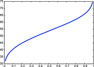
Figure 1: The estimated percentiles of the HEI-2005 total score. The horizontal axis is the percentile of interest, for example, $0.5$ refers to the median, while the vertical axis gives percentile of the HEI-2005 scores. Standard error estimates are given in Table 2.

Table 3 presents the first estimates of the distribution of HEI-2005 scores for a vulnerable subgroup of the population, namely, children aged 2–8 years. A previous analysis of 2003–2004 NHANES data, looking separately at 2–5 year olds and 6–11 year olds, was limited to estimates of mean usual HEI-2005 scores [59.6 and 54.7, respectively; see Fungwe et al. (2009)]. The mean scores noted here are comparable to those and reinforce the notion that children’s diets, on average, are far from ideal. However, this analysis provides a more complete picture of the state of US children’s diets. By including the scores at various percentiles, we estimate that only 5% of children have a score of 69 or greater and another 10% have scores of 41 or lower. While not in the table, we also estimate that the 99th percentile is $74$. This analysis suggests that virtually all children in the US have suboptimal diets and that a sizeable fraction (10%) have alarmingly low scores (41 or lower.)

We have also considered whether our multivariate model fitting procedure gives reasonable marginal answers. To check this, we note that it is possible to use the SAS procedure NLMIXED separately for each component to fit a model with one episodically consumed food group or daily consumed dietary component together with energy. The marginal distributions of each such component done separately are quite close to what we have reported in Table 3, as is our mean, which is $53.50$ compared to the mean of $53.25$ based on analyzing one HEI-2005 component at a time with the NLMIXED procedure. The only case where there is a mild discrepancy is in the estimated variability of the energy-adjusted usual intake of oils, likely caused by the NLMIXED procedure itself, which has an estimated variance $9$ times greater than our estimated variance.

Of course, it is the distribution of the HEI-2005 total score that cannot be estimated by analysis of one component at a time.

Table 4: Estimated correlation matrix for energy-adjusted usual intakes

Component	TF	WF	TV	DOL	TG	WG	Milk	Meat	Oil	SatFat	Sodium	SoFAAS
TF	1	$0.76$	$0.07$	$0.41$	$-0.10$	$0.33$	$0.16$	$0.08$	$-0.35$	$-0.38$	$-0.25$	$-0.64$
WF		$1$	$0.14$	$0.49$	$0.03$	$0.35$	$0.10$	$0.05$	$-0.17$	$-0.30$	$-0.20$	$-0.51$
TV			$1$	$0.51$	$-0.25$	$-0.23$	$-0.09$	$0.51$	$-0.08$	$0.08$	$0.42$	$-0.16$
DOL				$1$	$-0.08$	$0.11$	$0.14$	$0.25$	$-0.06$	$-0.23$	$0.01$	$-0.47$
TG					$1$	$0.30$	$-0.30$	$-0.13$	$0.44$	$-0.36$	$0.17$	$-0.22$
WG						$1$	$0.18$	$-0.18$	$-0.11$	$-0.29$	$-0.17$	$-0.46$
Milk							$1$	$-0.37$	$-0.21$	$0.21$	$-0.27$	$-0.21$
Meat and beans								$1$	$-0.06$	$-0.08$	$0.39$	$-0.19$
Oil									$1$	$-0.06$	$0.11$	$0.05$
SatFat										$1$	$0.09$	$0.46$
Sodium											$1$	$0.04$
SoFAAS												$1$

[]Here TF${}={}$Total Fruits, WF${}={}$Whole Fruits, TV${}={}$Total Vegetables, WG${}={}$Whole Grains, TG${}={}$Total Grains, SatFat${}={}$Saturated Fat. Here, “DOL” is dark green and orange vegetables and legumes. Also, “SoFAAS” is calories from solid fats, alcoholic beverages and added sugars. First 24 h Two 24 h Model BRR s.e. Total fruit $0.38$ $0.44$ $0.62$ 0.05 Whole fruit $0.31$ $0.37$ $0.59$ 0.10 Total vegetables $0.09$ $0.11$ $0.10$ 0.11 DOL $0.18$ $0.24$ $0.41$ 0.07 Total grains $0.00$ $0.00$ $0.06$ 0.11 Whole grains $0.12$ $0.16$ $0.53$ 0.08 Milk $-0.07$ $-0.01$ $0.01$ 0.08 Mean and beans $-0.03$ $-0.01$ $-0.03$ 0.15 Oil $0.08$ $0.05$ $-0.17$ 0.08 Saturated fat $0.21$ $0.23$ $0.36$ 0.06 Sodium $-0.03$ $0.05$ $0.07$ 0.12 SoFAAS $0.52$ $0.59$ $0.72$ 0.04 []The column labeled “Two 24 h” is the naive analysis that uses the mean of the two 24 h recalls, while the column labeled “First 24 h” is the naive analysis that uses the first 24 h recall. The column labeled “Model” is our analysis, and the column labeled “BRR s.e.” is the estimated standard error of our estimates. Here, “DOL” is dark green and orange vegetables and legumes. Also, “SoFAAS” is calories from solid fats, alcoholic beverages and added sugars.

Table 5: Estimated correlations between each individual HEI-2005 component score and the sum of the other HEI component scores, that is, the difference of the total score and each individual component

There are other things that have not been computed previously that are simple by-products of our analysis. For example, the correlations among energy-adjusted usual intakes involving episodically consumed foods have not been estimated previously, but this is easy for us; see Table 5. The estimated correlation of $-0.64$ between energy-adjusted total fruit and energy-adjusted SoFAAS, and the $-0.47$ correlation between DOL and SoFAAS are surprisingly high.

5.4 Component scores and other scores.

As described in the Introduction, an open problem has been to estimate the correlation between the individual score on each dietary component and the scores of all other dietary components. In their Table 3, Guenther et al. (2008) consider this problem, but of course they did not have a model for usual energy adjusted intakes, and instead they used a single 24 h recall. In Table 5 we show the resulting correlations using (a) a single 24 h recall; (b) the mean of two 24 h recalls for those who have two 24 h recalls; and (c) our model for usual intake. The numbers for the former differ from that of Guenther et al. (2008) because we are considering here a different population than do they. A striking and not unexpected aspect of this table is that for those components with nontrivial correlations, the correlations all increase as one moves from a single 24 h recall to the mean of two 24 h recalls and then finally to estimated usual intake. Thus, for example, the correlation between the HEI-2005 score for total fruit and its difference with the total score is 0.38 for a single 24 h recall, 0.44 for the mean of two 24 h recalls and then finally 0.62 for usual intake.

Table 6: Estimated distributions of energy-adjusted usual intake for those whose total HEI-2005 total scores are ${\leq}50$ and ${>}50$

			Percentile
Component	Mean	s.d.	5th	10th	25th	50th	75th	90th	95th
Whole fruit
Total score $\leq$50	$0.15$	0.12	$0.02$	$0.03$	$0.07$	$0.12$	$0.21$	$0.30$	$0.38$
Total score $>$50	$0.39$	0.22	$0.11$	$0.15$	$0.23$	$0.35$	$0.51$	$0.68$	$0.80$
Whole grains
Total score $\leq$50	$0.18$	0.13	$0.03$	$0.05$	$0.09$	$0.15$	$0.25$	$0.36$	$0.44$
Total score $>$50	$0.32$	0.20	$0.07$	$0.10$	$0.17$	$0.28$	$0.42$	$0.59$	$0.70$
DOL
Total score $\leq$50	$0.02$	0.02	$0.00$	$0.00$	$0.01$	$0.02$	$0.03$	$0.05$	$0.07$
Total score $>$50	$0.06$	0.05	$0.01$	$0.01$	$0.03$	$0.05$	$0.09$	$0.13$	$0.17$
SoFAAS
Total score $\leq$50	$42.43$	3.97	$36.40$	$37.59$	$39.66$	$42.16$	$44.92$	$47.67$	$49.42$
Total score $>$50	$33.83$	4.44	$26.01$	$27.89$	$30.97$	$34.15$	$36.98$	$39.28$	$40.57$
Total Score	$53.50$	9.58	$37.42$	$40.74$	$46.73$	$53.68$	$60.36$	$65.87$	$68.96$

[]Here, “DOL” is dark green and orange vegetables and legumes. Also, “SoFAAS” is calories from solid fats, alcoholic beverages and added sugars. Units of measurement are given in Table 2.

5.5 Distributions of intakes for subsets of HEI total scores.

A third open question is as follows: among those whose total HEI-2005 score is $>$50 or $\leq$50, what is the distribution of energy-adjusted usual intake of whole grains, whole fruits, dark green and orange vegetables and legumes (DOL) and calories from solid fats, alcoholic beverages and added sugars (SoFAAS)? This follows naturally from our method. Following (8), let $G_{1}(\widetilde{T}_{bi})$ be energy adjusted usual intake and let $G_{2}(\widetilde{T}_{bi})$ be the HEI total score. Then the distributions in question for when the total HEI-2005 score is $>$50 can be estimated as $\widehat{F}(x)=\sum_{i=1}^{n}\sum_{b=1}^{B}w_{i}I\{G_{1}(\widetilde{T}_{bi})\leq x\}I\{G_{2}(\widetilde{T}_{bi})>50\}/\sum_{i=1}^{n}\sum_{b=1}^{B}w_{i}I\{G_{2}(\widetilde{T}_{bi})>50\}$.

The results are provided in Table 6, with a graphical view in Figure 2. The results show that those who have poorer diets with usual HEI-2005 total score $\leq 50$ are consistently eating poorer diets, that is, less whole fruits, less whole grains and less DOL, but higher SoFAAS.

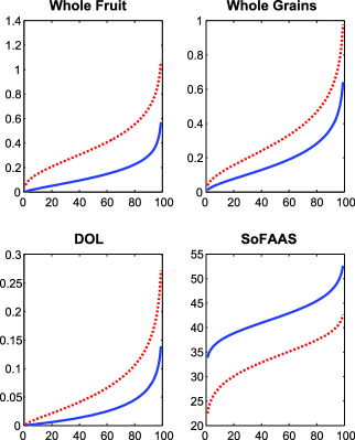
Figure 2: The estimated percentiles of the energy-adjusted usual intakes for Whole fruits (top left) in cups/(1,000 kcal), Whole grains (top right) in ounces/(1,000 kcal), DOL (bottom left) in cups/ (1,000 kcal) and calories from SoFAAS (bottom right) in % of Energy. The solid lines are for those whose usual HEI-2005 total score is $\leq$50, that is, poorer diets, while the dashed lines are for those whose usual HEI-2005 total score is $>$50, that is, better diets.

5.6 Dietary consistency.

We stated in the Introduction that it is interesting to understand the percentage of children whose usual intake HEI score exceeds the median HEI score on all 12 HEI components. Those median scores, say, $(\kappa_{1},\ldots,\kappa_{12})$, are estimated in Table 3. If $G_{j}(\widetilde{T}_{bi})$ is the HEI component score for episodically consumed food $j$, then following (8) the quantity in question can be estimated as $\sum_{i=1}^{n}\sum_{b=1}^{B}w_{i}\prod_{j=1}^{6}I\{G_{j}(\widetilde{T}_{bi})\geq\kappa_{j}\}/\sum_{i=1}^{n}\sum_{b=1}^{B}w_{i}$. We estimate that the percentage is 6%, woefully small. The percentage of children whose usual intake HEI score exceeds the median HEI score on all 12 HEI components is 0.24%. Figure 3 gives the estimated probabilities of exceeding the $\kappa$ percentile on all 12 HEI components simultaneously, for $\kappa=1,2,\ldots,99$.

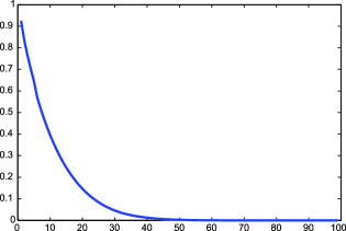
Figure 3: The Y-axis gives the estimated probabilities of exceeding the $\kappa$ (X-axis) percentile on all 12 HEI components, for $\kappa=1,2,\ldots,99$; see Section 5.6.

5.7 Uncertainty quantification.

The BRR standard errors of HEI-2005 components’ adjusted usual intakes and scores are shown in Tables 2 and 3. The BRR weights are only used in variance calculations. Once we have estimated some quantity, say, $\widehat{\theta}$, from the sample using sample weight, we will need to compute the same quantity using, in succession, the 32 BRR weights. This will give us 32 estimates $\widehat{\theta}_{1},\widehat{\theta}_{2},\ldots,\widehat{\theta}_{32}$. The BRR estimate for the variance of $\widehat{\theta}$ is $(32\times 0.49)^{-1}\sum_{p=1}^{32}(\widehat{\theta}_{p}-\widehat{\theta})^{2}$. The 32 in the denominator is for the 32 different estimates from the 32 different sets of weights, and the $0.49$ is the square of the perturbation factor used to construct the BRR weight sets [Wolter (1995)].

6 Further discussion of the analysis.

6.1 Never consumers.

An aspect of the modeling that we have not discussed is the possibility that some people never, ever consume an episodically consumed dietary component. Our model does not allow for this, for general reasons and for reasons that are specific to our data analysis.

It is in principle possible to add an additional modeling step for nonconsumers, via fixed effects probit regression, but we do not think this is a practical issue in our case, for two reasons:

• The first is that the HEI-2005 is based on 6 episodically consumed dietary components, namely, total fruit, whole fruit, whole grains, total vegetables, DOL and milk, the latter of which includes cheese, yogurt and soy beverages. None of these are “lifestyle adverse,” unlike, say, alcohol. While 40% of the responses for whole fruits, for example, equal zero, the percentage of children who never eat any whole fruits at all is likely to be minuscule.

• Even if one disputes whether there are very few individuals who never consume one of the dietary components, then it necessarily follows that we have overestimated the HEI-2005 total scores, and, hence, the estimates of the proportion of individuals with alarmingly low HEI scores are deflated, and not inflated. The reason is that our model suggests everyone has a positive usual intake of the 6 episodically consumed dietary components. Since the HEI-2005 score components are nondecreasing functions of usual intake of the episodically consumed dietary components, this would mean that we overestimate the HEI-2005 total score.

6.2 Computing and data.

Our programs were written in Matlab. The programs, along with the NHANES data we used, are available in the Annals of Applied Statistics online archive. Although a much smaller amount of computing effort yields similar results, using 70,000 MCMC steps with a burn-in of 20,000 takes approximately 10 hours on a Linux server.

We also estimated the Monte Carlo standard error which is defined by Flegal, Haran and Jones (2008) as $\widehat{\sigma}_{g}/\sqrt{n}$, where $n$ is the total of iterations, and $n=ab$, where $a$ is the number of blocks and $b$ is the block size, and where

$$\bar{Y_{j}}=b^{-1}\sum_{i={(j-1)b+1}}^{jb}g(X_{i})\qquad\mbox{for }j=1,\ldots,a.$$

The batch means estimate of $\sigma_{g}^{2}$ is

$$\widehat{\sigma}_{g}^{2}=\frac{b}{a-1}\sum_{j=1}^{a}(\bar{Y}_{j}-\bar{g}_{n})^{2}.\vspace*{-1pt}$$

The ratio of the Monte Carlo standard error to the estimated standard deviation of the estimated parameters averages $3.4\%$ for $\Sigma_{u}$ and $1.7\%$ for $\beta$.

Because of the public health importance of the problem, the National Cancer Institute has contracted for the creation of a SAS program that performs our analysis. It will allow any number of episodically and daily consumed dietary components. The first draft of this program, written independently in a different programming language, gives almost identical results to what we have obtained, at least suggesting that our results are not the product of a programming error.

7 Discussion.

7.1 Transformations.

In Appendix .15 we describe how we estimated the transformation parameters as a separate component-wise calculation. We have done some analyses where we simultaneously transform each component, and found very little difference with our results. However, the comp-

uting time to implement this is extremely high, because of the fact that different transformations make data on different scales, so we have to compute the usual intakes at each step in the MCMC, and not just at the end.

7.2 What have we learned that is new.

There are many important questions in dietary assessment that have not been able to be answered because of a lack of multivariate models for complex, zero-inflated data with measurement errors and a lack of ability to fit such multivariate models. Nutrients and foods are not consumed in isolation, but rather as part of a broader pattern of eating. There is reason to believe that these various dietary components interact with one another in their effect on health, sometimes working synergistically and sometimes in opposition. Nonetheless, simply characterizing various patterns of eating has presented enormous statistical challenge. Until now, descriptive statistics on the HEI-2005 have been limited to examination of either the total scores or only a single energy-adjusted component at a time. This has precluded characterization of various patterns of dietary quality as well as any subsequent analyses of how such patterns might relate to health.

This methodology presented in this paper presents a workable solution to these problems which has already proven valuable. In May 2010, just as we were submitting the paper, a White House Task Force on Childhood Obesity created a report. They had wanted to set a goal of all children having a total HEI score of 80 or more by 2030, but when they learned we estimated only 10% of the children ages 2–8 had a score of 66 or higher, they decided to set a more realistic target. The facility to estimate distributions of the multiple component scores simultaneously will be important in tracking progress toward that goal.

7.3 In what other arenas will our work have impact?

There are many other important problems where multivariate models such as ours will be important. One such problem arises when studying the relationship between multiple dietary components or dietary patterns and health outcomes. Traditionally, for cost reasons, large cohort studies have used a food frequency questionnaire (FFQ) to measure dietary intake, sometimes with a small calibration study including short-term measures such as 24 h recalls. However, there is a new web-based instrument called the Automated Self-administered 24-hour Dietary Recall (ASA24^TM) (see http://riskfactor.cancer.gov/tools/instruments/asa24), which has been proposed to replace or at least supplement the FFQ and which is currently undergoing extensive testing. The dietary data we will see then is what we have called $Y_{ijk}$, that is, 24 h recall data. In order to correct relative risk estimates for the measurement error inherent in the ASA24^TM, regression calibration [Carroll et al. (2006)] will almost certainly be the method of choice, as it is in most of nutritional epidemiology. This method attempts to produce an estimate of the regression of usual intake on the observed intakes, and then to use these estimates in Cox and logistic regression for the health outcome. In order to perform this regression, a multivariate measurement error model will be required, since the regression is on all the observed dietary intake components in the regression model measured by the ASA24^TM, and not on each individual component. Our methodology is easily extended to address this problem.

Appendix: Details of the fitting procedure

In this Appendix we give the full details of the model fitting procedure.

.4 Notational convention.

In our example, age was standardized to have mean $0.0$ and variance $1.0$, to improve numerical stability.

As described in Section 3.1, the observed, transformed nonzero 24 h recalls were standardized to have mean $0.0$ and variance $2.0$. More precisely, for $\ell=1,2,\ldots,6$, we first transformed the nonzero food group data as $Z_{i,2\ell,k}=g(Y_{i,2\ell,k},\lambda_{\ell})$, and then we standardized these data as $Q_{i,2\ell,k}=\sqrt{2}\{Z_{i,2\ell,k}-\mu(\lambda_{\ell})\}/\sigma(\lambda_{\ell})$, where $\{\mu(\lambda_{\ell}),\sigma(\lambda_{\ell})\}$ are the mean and standard deviation of the nonzero food intakes $Z_{i,2\ell,k}$. Similarly, for nonepisodically consumed dietary components and energy we transformed to $Z_{i,6+\ell,k}=g(Y_{i,6+\ell,k},\lambda_{\ell})$ for $\ell=7,\ldots,13$, and then standardized to $Q_{i,6+\ell,k}=\sqrt{2}\{Z_{i,6+\ell,k}-\mu(\lambda_{\ell})\}/\sigma(\lambda_{\ell})$. Of course, whether the food group is consumed or not is $Q_{i,2\ell-1,k}=Y_{i,2\ell-1,k}$ for $\ell=1,\ldots,6$. Collected, the data are $\widetilde{Q}_{ik}=(Q_{ijk})_{j=1}^{19}$. The terms $\{\mu(\lambda_{\ell}),\break\sigma(\lambda_{\ell})\}$ are not random variables but are merely constants used for standardization, and we need not consider inference for them. Back-transformation is discussed in Appendix .14.

.5 Prior distributions.

Because the data were standardized, we used the following conventions:

• The prior for all $\beta_{j}$ were normal with mean zero and variance $100$.

• The prior for $\Sigma_{u}$ was exchangeable with diagonal entries all equal to $1.0$ and correlations all equal to $0.50$. There were 21 degrees of freedom in the inverse Wishart prior, that is, $m_{u}=21$. Thus, the prior is $\mathrm{IW}\{(m_{u}-19-1)\Sigma_{u,\mathrm{prior}},m_{u}\}$. We experimented with this prior by using zero correlation, and the results were essentially unchanged.

• The prior for $r_{k}$ is $\operatorname{Uniform}[-1,1]$. Set the initial value: $r_{k}=0$, $k=1,\ldots,5$.

• The prior for $\theta_{k}$ is $\operatorname{Uniform}[-\pi,\pi]$. Set the initial value: $\theta_{k}=0$, $k=1,\ldots,25$.

• The priors for $v_{22},v_{44},\ldots,v_{12,12}$ and $v_{13,13},\ldots,v_{19,19}$ were $\operatorname{Uniform}[-3,3]$. Set the initial values: $v_{22}=v_{44}=\cdots=v_{12,12}=v_{13,13}=\cdots=v_{19,19}=1$.

• For the rest of the nondiagonal $v_{ij}$’s which could not be determined by the restrictions, we used $\operatorname{Uniform}[-3,3]$ priors. Set the initial values to be 0.

The constraints on $\Sigma_{\varepsilon}$ are nonlinear, and our parameterization enforces them easily without having to have prior distributions for the original parameterization that satisfy the nonlinear constraints.

The key thing that makes things work well with the other components of the matrix $V$ with $\Sigma_{\varepsilon}=VV^{\mathrm{T}}$ is that we have standardized the data as described in Appendix .4. With this standardization, things become much nicer. For example, the variance of the $\varepsilon$’s for energy is $\sum_{j=1}^{19}v_{19,j}^{2}$. However, since the sample variance for energy is standardized to equal $2.0$, we simply just need to make priors for $v_{19,j}$ be uniform on a modest range to have real flexibility.

.6 Generating starting values for the latent variables.

While we observe $\widetilde{Q}_{ik}$, in the MCMC we need to generate starting values for the latent variables $\widetilde{W}_{ik}=(W_{ijk})_{j=1}^{19}$ to initiate the MCMC:

• For nutrients and energy, $Q_{ijk}=W_{ijk}$, no data need be generated, $j=13,\ldots,19$.

• For the amounts, $Q_{i2k}$, $Q_{i4k}$, $Q_{i6k}$, $Q_{i8k}$, $Q_{i,10,k}$ and $Q_{i,12,k}$, we set $W_{i2k}=Q_{i2k}$, $W_{i4k}=Q_{i4k}$, $W_{i6k}=Q_{i6k}$, $W_{i8k}=Q_{i8k}$, $W_{i,10,k}=Q_{i,10,k}$ and $W_{i,12,k}=Q_{i,12,k}$.

• For consumption, we generate $\widetilde{U}_{i}$ as normally distributed with mean zero and covariance matrix given as the prior covariance matrix for $\Sigma_{u}$. For $\ell=1,\ldots,6$, we also compute $z_{ik}=|X_{i,2\ell-1,k}^{\mathrm{T}}\beta_{2\ell-1,\mathrm{prior}}+U_{i,2\ell-1}+\mathcal{Z}_{ik}|$, where $\mathcal{Z}_{ik}=\operatorname{Normal}(0,1)$ are generated independently. We then set $W_{i,2\ell-1,k}=z_{ik}Q_{i,2\ell-1,k}-z_{ik}(1-Q_{i,2\ell-1,k})$.

• Finally, we then updated $\widetilde{W}_{ik}$ by a single application of the updates given in Appendix .12.

.7 Complete data loglikelihood.

Let $J=19$. The complete data include the indicators of whether a food was consumed, the $W$ variables and the random effect $U$ variables. The loglikelihood of the complete data is

$$\sum_{\ell=1}^{6}\sum_{i=1}^{n}\sum_{k=1}^{m_{i}}\log\{Q_{i,2\ell-1,k}I(W_{i,2\ell-1,k}>0)$$

$$\hphantom{\sum_{\ell=1}^{6}\sum_{i=1}^{n}\sum_{k=1}^{m_{i}}\log\{}{}+(1-Q_{i,2\ell-1,k})I(W_{i,2\ell-1,k}<0)\}$$

$$\qquad{}+\Biggl{(}\sum_{i=1}^{n}w_{i}/2\Biggr{)}\log(|\Sigma_{u}^{-1}|)-(1/2)\sum_{i=1}^{n}w_{i}\widetilde{U}_{i}^{\mathrm{T}}\Sigma_{u}^{-1}\widetilde{U}_{i}$$

$$\qquad{}-(1/2)\sum_{j=1}^{J}(\beta_{j}-\beta_{j,\mathrm{prior}})^{\mathrm{T}}\Omega_{\beta,j}^{-1}(\beta_{j}-\beta_{j,\mathrm{prior}})$$

$$\qquad{}+\{(m_{u}+J+1)/2\}\log(|\Sigma_{u}^{-1}|)-\{(m_{u}-J-1)/2\}\operatorname{trace}(\Sigma_{u,\mathrm{prior}}\Sigma_{u}^{-1})$$

$$\qquad{}-(1/2)\sum_{i=1}^{n}w_{i}m_{i}\log\{(v_{22}^{2}v_{44}^{2}v_{66}^{2}v_{88}^{2}v_{10,10}^{2}v_{12,12}^{2}v_{13,13}^{2}\cdots v_{JJ}^{2})\prod_{q=1}^{5}(1-r_{q}^{2})\}$$

$$\qquad{}-(1/2)\sum_{i=1}^{n}w_{i}\sum_{k=1}^{m_{i}}\{\widetilde{W}_{ik}-(X_{i1k}^{\mathrm{T}}\beta_{1},\ldots,X_{iJk}^{\mathrm{T}}\beta_{J})^{\mathrm{T}}-\widetilde{U}_{i}\}^{\mathrm{T}}\Sigma_{\varepsilon}^{-1}$$

$$\hphantom{\qquad{}-(1/2)\sum_{i=1}^{n}w_{i}\sum_{k=1}^{m_{i}}}{}\times\{\widetilde{W}_{ik}-(X_{i1k}^{\mathrm{T}}\beta_{1},\ldots,X_{iJk}^{\mathrm{T}}\beta_{J})^{\mathrm{T}}-\widetilde{U}_{i}\}.$$

We used Gibbs sampling to update this complete data loglikelihood, the details for which are given in subsequent appendices. The weights $w_{i}$ are integers and are used here in a pseudo-likelihood fashion. One can also think of this as expanding each individual into $w_{i}$ individuals, each with the same observed data but different latent variables. For computational convenience, since we are only asking for a frequentist estimator and not doing full Bayesian inference, the latent variables in the process are generated once for each individual. Estimates of $\Sigma_{u}$, $\Sigma_{\varepsilon}$ and $\beta_{j}$ for $j=1,\ldots,J$ were computed as the means from the Gibbs samples. Once again, we emphasize that we are not doing a proper Bayesian analysis, but only using MCMC techniques to obtain a frequentist estimate, with uncertainty assessed using the frequentist BRR method.

.8 Complete conditionals for $r_{q}$, $\theta_{q}$ and $v_{pq}$.

Except for irrelevant constants, the complete conditional for $r_{q}$ ($q=1,\ldots,5$) is

$$\log[r_{q}|\mathrm{rest}] = -\frac{1}{2}\sum_{i=1}^{n}w_{i}m_{i}\log(1-r_{q}^{2})$$

$${}-\frac{1}{2}\sum_{i=1}^{n}w_{i}\sum_{k=1}^{m_{i}}\{\widetilde{W}_{ik}-(X_{i1k}^{\mathrm{T}}\beta_{1},\ldots,X_{i,19,k}^{\mathrm{T}}\beta_{19})^{\mathrm{T}}-\widetilde{U}_{i}\}^{\mathrm{T}}$$

$$\hphantom{{}-\frac{1}{2}\sum_{i=1}^{n}w_{i}\sum_{k=1}^{m_{i}}}{}\times\Sigma_{\varepsilon}^{-1}\{\widetilde{W}_{ik}-(X_{i1k}^{\mathrm{T}}\beta_{1},\ldots,X_{i,19,k}^{\mathrm{T}}\beta_{19})^{\mathrm{T}}-\widetilde{U}_{i}\}.$$

Except for irrelevant constants, the complete conditionals for $v_{qq}$ ($q=2,4,6,8,10,12,13,\ldots,19$) are

$$\log[v_{qq}|\mathrm{rest}] = -\frac{1}{2}\sum_{i=1}^{n}w_{i}m_{i}\log(v_{qq}^{2})$$

$${}-\frac{1}{2}\sum_{i=1}^{n}w_{i}\sum_{k=1}^{m_{i}}\{\widetilde{W}_{ik}-(X_{i1k}^{\mathrm{T}}\beta_{1},\ldots,X_{i,19,k}^{\mathrm{T}}\beta_{19})^{\mathrm{T}}-\widetilde{U}_{i}\}^{\mathrm{T}}$$

$$\hphantom{{}-\frac{1}{2}\sum_{i=1}^{n}w_{i}\sum_{k=1}^{m_{i}}}{}\times\Sigma_{\varepsilon}^{-1}\{\widetilde{W}_{ik}-(X_{i1k}^{\mathrm{T}}\beta_{1},\ldots,X_{i,19,k}^{\mathrm{T}}\beta_{19})^{\mathrm{T}}-\widetilde{U}_{i}\}.$$

Except for irrelevant constants, the compete conditionals for $\theta_{q}$ ($q=1,\ldots,25$) and nondiagonal free parameters $v_{pq}$ are

$$\log[x|\mathrm{rest}] = -\frac{1}{2}\sum_{i=1}^{n}w_{i}\sum_{k=1}^{m_{i}}\{\widetilde{W}_{ik}-(X_{i1k}^{\mathrm{T}}\beta_{1},\ldots,X_{i,19,k}^{\mathrm{T}}\beta_{19})^{\mathrm{T}}-\widetilde{U}_{i}\}^{\mathrm{T}}$$

$$\hskip 71.13188pt\times\Sigma_{\varepsilon}^{-1}\{\widetilde{W}_{ik}-(X_{i1k}^{\mathrm{T}}\beta_{1},\ldots,X_{i,19,k}^{\mathrm{T}}\beta_{19})^{\mathrm{T}}-\widetilde{U}_{i}\}.$$

The full conditionals do not have an explicit form, so we use a Metropolis–Hastings within a Gibbs sampler to generate it:

• $r_{q}$ ($q=1,\ldots,5$). We discretize the values of $r_{q}$ to the set $\{-0.99+2\times 0.99(j-1)/(M-1)\}$, where $j=1,\ldots,M$ and we choose $M=41$.

  Proposal: The current value is $r_{q,t}$. The proposed value of $r_{q,t+1}$ is selected randomly from the current value and the two nearest neighbors of $r_{q,t}$. Then $r_{q,t+1}$ is accepted with probability $\min\{1,g(r_{q,t+1})/g(r_{q,t})\}$, where

  $$g(y) \propto (1-y^{2})^{-{1}/{2}\sum_{i=1}^{n}w_{i}m_{i}}$$

  $${}\!\!\!\times\exp\Biggl{[}\!-\frac{1}{2}\sum_{i=1}^{n}w_{i}\!\sum_{k=1}^{m_{i}}\{\widetilde{W}_{ik}\!-\!(X_{i1k}^{\mathrm{T}}\beta_{1},\ldots,X_{i,19,k}^{\mathrm{T}}\beta_{19})^{\mathrm{T}}\!-\!\widetilde{U}_{i}\}^{\mathrm{T}}\Sigma_{\varepsilon}^{-1}(\bullet)\Biggr{]}\!,$$

  where here and in what follows, for any $A$, $A^{\mathrm{T}}\Sigma_{\varepsilon}^{-1}(\bullet)=A^{\mathrm{T}}\Sigma_{\varepsilon}^{-1}A$.

• $\theta_{q}$ ($q=1,\ldots,25$). We discretize similarly as above.

  Proposal: The current value is $\theta_{q,t}$. The proposed value $\theta_{q,t+1}$ is selected randomly from the current value and the two nearest neighbors of $\theta_{q,t}$. Then $\theta_{q,t+1}$ is accepted with probability $\min\{1,g(\theta_{q,t+1})/g(\theta_{q,t})\}$, where

  $$g(y)\propto\exp\Biggl{[}-\frac{1}{2}\sum_{i=1}^{n}w_{i}\sum_{k=1}^{m_{i}}\{\widetilde{W}_{ik}-(X_{i1k}^{\mathrm{T}}\beta_{1},\ldots,X_{i,19,k}^{\mathrm{T}}\beta_{19})^{\mathrm{T}}-\widetilde{U}_{i}\}^{\mathrm{T}}\Sigma_{\varepsilon}^{-1}(\bullet)\Biggr{]}.$$

• $v_{qq}$ ($q=2,4,6,8,10,12,13,\ldots,19$). Proposal: The current value is $v_{qq,t}$. A candidate $v_{qq,t+1}$ is generated from the Uniform distribution of length 0.4 with mean $v_{qq,t}$. The candidate value $v_{qq,t+1}$ is accepted with probability $\min\{1,g(v_{qq,t+1})/g(v_{qq,t})\}$, where

  $$g(y) \propto y^{-\sum_{i=1}^{n}w_{i}m_{i}}$$

  $${}\!\!\!\times\exp\Biggl{[}\!-\frac{1}{2}\sum_{i=1}^{n}w_{i}\!\sum_{k=1}^{m_{i}}\{\widetilde{W}_{ik}\!-\!(X_{i1k}^{\mathrm{T}}\beta_{1},\ldots,X_{i,19,k}^{\mathrm{T}}\beta_{19})^{\mathrm{T}}\!-\!\widetilde{U}_{i}\}^{\mathrm{T}}\Sigma_{\varepsilon}^{-1}(\bullet)\Biggr{]}\!.$$

• Nondiagonal free parameters $v_{pq}$. Proposal: The current value is $v_{pq,t}$. The candidate value $v_{pq,t+1}$ is generated from the Uniform distribution of length 0.4 with mean $v_{pq,t}$. The candidate value is accepted with probability $\min\{1,g(v_{pq,t+1})/g(v_{pq,t})\}$, where

  $$g(y)\propto\exp\Biggl{[}-\frac{1}{2}\sum_{i=1}^{n}w_{i}\sum_{k=1}^{m_{i}}\{\widetilde{W}_{ik}-(X_{i1k}^{\mathrm{T}}\beta_{1},\ldots,X_{i,19,k}^{\mathrm{T}}\beta_{19})^{\mathrm{T}}-\widetilde{U}_{i}\}^{\mathrm{T}}\Sigma_{\varepsilon}^{-1}(\bullet)\Biggr{]}.$$

.9 Complete conditionals for $\Sigma_{u}$.

The dimension of the covariance matrices is $J=19$. By inspection, the complete conditional for $\Sigma_{u}$ is

$$[\Sigma_{u}|\mathrm{rest}]=\mathrm{IW}\Biggl{\{}(m_{u}-J-1)\Sigma_{u,\mathrm{prior}}+\sum_{i=1}^{n}w_{i}\widetilde{U}_{i}\widetilde{U}_{i}^{\mathrm{T}},n+m_{u}\Biggr{\}},$$

where here $\mathrm{IW}=\mathrm{the}$ Inverse-Wishart distribution. The density of $\mathrm{IW}(\Omega,m)$ for a $J\times J$ random variable is

$$\mathrm{IW}(\Omega,m)=f(Q|\Omega,m)\propto|Q|^{-(m+J+1)/2}\exp\bigl{\{}-\tfrac{1}{2}\operatorname{trace}(\Omega Q^{-1})\bigr{\}}.$$

This has expectation $\Omega/(m-J-1)$.

.10 Complete conditionals for $\beta$.

Let the elements of $\Sigma_{\varepsilon}^{-1}$ be $\sigma_{\varepsilon}^{j\ell}$. For any $j$, except for irrelevant constants,

$$\log[\beta_{j}|\mathrm{rest}] = -\frac{1}{2}(\beta_{j}-\beta_{j,\mathrm{prior}})^{\mathrm{T}}\Omega_{\beta,j}^{-1}(\beta_{j}-\beta_{j,\mathrm{prior}})$$

$${}-\frac{1}{2}\sum_{i=1}^{n}w_{i}\sum_{k=1}^{m_{i}}(W_{ijk}-X_{ijk}^{\mathrm{T}}\beta_{j}-U_{ij})^{2}\sigma_{\varepsilon}^{jj}$$

$${}-\sum_{i=1}^{n}w_{i}\sum_{k=1}^{m_{i}}\sum_{\ell\neq j}\sigma_{\varepsilon}^{j\ell}(W_{ijk}-X_{ijk}^{\mathrm{T}}\beta_{j}-U_{ij})(W_{i\ell k}-X_{i\ell k}^{\mathrm{T}}\beta_{\ell}-U_{i\ell})$$

$$= \mathcal{C}_{1}^{\mathrm{T}}\beta_{j}-\frac{1}{2}\beta_{j}^{\mathrm{T}}\mathcal{C}_{2}^{-1}\beta_{j},$$

which implies $[\beta_{j}|\mathrm{rest}]=\operatorname{Normal}(\mathcal{C}_{2}\mathcal{C}_{1},\mathcal{C}_{2})$, where

$$\mathcal{C}_{2} = \Biggl{(}\Omega_{\beta,j}^{-1}+\sum_{i=1}^{n}w_{i}\sigma_{\varepsilon}^{jj}\sum_{k=1}^{m_{i}}X_{ijk}X_{ijk}^{\mathrm{T}}\Biggr{)}^{-1};$$

$$\mathcal{C}_{1} = \Omega_{\beta,j}^{-1}\beta_{j,\mathrm{prior}}+\sum_{i=1}^{n}w_{i}\sum_{k=1}^{m_{i}}\sigma_{\varepsilon}^{jj}X_{ijk}(W_{ijk}-U_{ij})$$

$${}+\sum_{i=1}^{n}w_{i}\sum_{k=1}^{m_{i}}\sum_{\ell\neq j}\sigma_{\varepsilon}^{j\ell}(W_{i\ell k}-X_{i\ell k}^{\mathrm{T}}\beta_{\ell}-U_{i\ell})X_{ijk}.$$

.11 Complete conditionals for $\widetilde{U}_{i}$.

The NHANES 2001–2004 weights are integers, representing the number of children that each sampled child represents. Thus, as described therein, the loglikelihood in Section .7 could also be rewritten equivalently by developing $w_{i}$ pseudo-children, each with the same observed data values. It thus does not make sense to use the weights to generate an individual $\widetilde{U}_{i}$. Instead, as described in Section .7, for computational convenience for generating a $\widetilde{U}_{i}$ to represent $w_{i}$ children, we set the weight for that child temporarily $=1.0$. Then, except for irrelevant constants,

$$\log[\widetilde{U}_{i}|\mathrm{rest}] = -\frac{1}{2}w_{i}\widetilde{U}_{i}^{\mathrm{T}}\Sigma_{u}^{-1}\widetilde{U}_{i}$$

$${}-\frac{1}{2}w_{i}\sum_{k=1}^{m_{i}}\{\widetilde{W}_{ik}-(X_{i1k}^{\mathrm{T}}\beta_{1},\ldots,X_{i,19,k}^{\mathrm{T}}\beta_{19})^{\mathrm{T}}-\widetilde{U}_{i}\}^{\mathrm{T}}\Sigma_{\varepsilon}^{-1}$$

$$\hphantom{{}-\frac{1}{2}w_{i}\sum_{k=1}^{m_{i}}}{}\times\{\widetilde{W}_{ik}-(X_{i1k}^{\mathrm{T}}\beta_{1},\ldots,X_{i,19,k}^{\mathrm{T}}\beta_{19})^{\mathrm{T}}-\widetilde{U}_{i}\}$$

$$= \mathcal{C}_{1}^{\mathrm{T}}\widetilde{U}_{i}-\frac{1}{2}\widetilde{U}_{i}^{\mathrm{T}}\mathcal{C}_{2}^{-1}\widetilde{U}_{i}.$$

Remembering that for purposes of this section we are setting $w_{i}=1.0$, this implies that $[\widetilde{U}_{i}|\mathrm{rest}]=\operatorname{Normal}(\mathcal{C}_{2}\mathcal{C}_{1},\mathcal{C}_{2})$, where

$$\mathcal{C}_{2} = (\Sigma_{u}^{-1}+m_{i}\Sigma_{\varepsilon}^{-1})^{-1};$$

$$\mathcal{C}_{1} = \sum_{k=1}^{m_{i}}\Sigma_{\varepsilon}^{-1}\{\widetilde{W}_{ik}-(X_{i1k}^{\mathrm{T}}\beta_{1},\ldots,X_{i,19,k}^{\mathrm{T}}\beta_{19})^{\mathrm{T}}\}.$$

.12 Complete conditional for $W_{i\ell k}$, $\ell=1,3,5,7,9,11$.

Here we do the complete conditional for $W_{i\ell k}$ with $\ell=1,3,5,7,9,11$. Except for irrelevant constants,

$$\log[W_{i\ell k}|\mathrm{rest}] = \log\{Q_{i\ell k}I(W_{i\ell k}>0)+(1-Q_{i\ell k})I(W_{i\ell k}<0)\}$$

$${}-\frac{1}{2}w_{i}(W_{i1k}-X_{i1k}^{\mathrm{T}}\beta_{1}-U_{i1},\ldots,W_{i,19,k}-X_{i,19,k}^{\mathrm{T}}\beta_{19}-U_{i,19})$$

$$\hphantom{{}-}{}\times\Sigma^{-1}_{\varepsilon}(\bullet)^{\mathrm{T}}$$

$$= \log\{Q_{i\ell k}I(W_{i\ell k}>0)+(1-Q_{i\ell k})I(W_{i\ell k}<0)\}$$

$${}-\frac{1}{2}w_{i}\sigma_{\varepsilon}^{\ell\ell}(W_{i\ell k}-X_{i\ell k}^{\mathrm{T}}\beta_{\ell}-U_{i\ell})^{2}$$

$${}-w_{i}\sum_{j\neq\ell}\sigma_{\varepsilon}^{\ell j}(W_{i\ell k}-X_{i\ell k}^{\mathrm{T}}\beta_{\ell}-U_{i\ell})(W_{ijk}-X_{ijk}^{\mathrm{T}}\beta_{j}-U_{ij})$$

$$= \log\{Q_{i\ell k}I(W_{i\ell k}>0)+(1-Q_{i\ell k})I(W_{i\ell k}<0)\}+\mathcal{C}_{1}W_{i\ell k}$$

$${}-\frac{1}{2}W_{i\ell k}^{2}\mathcal{C}_{2}^{-1},$$

where, using the convention of Appendix .11,

$$\mathcal{C}_{2} = 1/(\sigma_{\varepsilon}^{\ell\ell})$$

$$\mathcal{C}_{1} = \sigma_{\varepsilon}^{\ell\ell}(X_{i\ell k}^{\mathrm{T}}\beta_{\ell}+U_{i\ell})-\sum_{j\neq\ell}\sigma_{\varepsilon}^{\ell j}(W_{ijk}-X_{ijk}^{\mathrm{T}}\beta_{j}-U_{ij}).$$

If we use the notation $\mathrm{TN}_{+}(\mu,\sigma,c)$ for a normal random variable with mean $\mu$ and standard deviation $\sigma$ that is truncated from the left at $c$, and similarly use $\mathrm{TN}_{-}(\mu,\sigma,c)$ when truncation is from the right at $c$, then it follows that with $\mu=\mathcal{C}_{2}\mathcal{C}_{1}$ and $\sigma=\mathcal{C}_{2}^{1/2}$,

$$[W_{i\ell k}|\mathrm{rest}] = Q_{i\ell k}\mathrm{TN}_{+}(\mu,\sigma,0)+(1-Q_{i\ell k})\mathrm{TN}_{-}(\mu,\sigma,0)$$

$$= \mu+Q_{i\ell k}\mathrm{TN}_{+}(0,\sigma,-\mu)+(1-Q_{i\ell k})\mathrm{TN}_{-}(0,\sigma,-\mu)$$

$$= \mu+Q_{i\ell k}\mathrm{TN}_{+}(0,\sigma,-\mu)-(1-Q_{i\ell k})\mathrm{TN}_{+}(0,\sigma,\mu)$$

$$= \mu+\sigma\{Q_{i\ell k}\mathrm{TN}_{+}(0,1,-\mu/\sigma)-(1-Q_{i\ell k})\mathrm{TN}_{+}(0,1,\mu/\sigma)\}.$$

Generating $\mathrm{TN}_{+}(0,1,c)$ is easy: if $c<0$, simply do rejection sampling of a $\operatorname{Normal}(0,1)$ until you get one that is $>c$. If $c>0$, there is an adaptive rejection scheme [Robert (1995)].

.13 Complete conditionals for $W_{i2k}$, $W_{i4k}$, $W_{i6k}$, $W_{i8k}$, $W_{i,10,k}$ and $W_{i,12,k}$ when not observed.

For $p=2,4,6,8,10,12$, the variable $W_{ipk}$ is not observed when $Q_{i,p-1,k}=0$, or, equivalently, when $W_{i,p-1,k}<0$. Except for irrelevant constants,

$$\log[W_{ipk}|\mathrm{rest}] = -\frac{1}{2}w_{i}\sum_{j}\sum_{\ell}\sigma_{\varepsilon}^{j\ell}(W_{ijk}-X_{ijk}^{\mathrm{T}}\beta_{j}-U_{ij})(W_{i\ell k}-X_{i\ell k}^{\mathrm{T}}\beta_{\ell}-U_{i\ell})$$

$$= -\frac{1}{2}W_{ipk}^{2}\mathcal{C}_{2}^{-1}+\mathcal{C}_{1}W_{ipk},$$

where, using the convention of Appendix .11,

$$\mathcal{C}_{2} = 1/(\sigma_{\varepsilon}^{pp});$$

$$\mathcal{C}_{1} = \sigma_{\varepsilon}^{pp}(X_{ipk}^{\mathrm{T}}\beta_{p}+U_{ip})-\sum_{\ell\neq p}\sigma_{\varepsilon}^{p\ell}(W_{i\ell k}-X_{i\ell k}^{\mathrm{T}}\beta_{\ell}-U_{i\ell}).$$

Therefore,

$$[W_{ipk}|\mathrm{rest}]=Q_{ipk}Q_{i,p-1,k}+(1-Q_{i,p-1,k})\operatorname{Normal}(\mathcal{C}_{2}\mathcal{C}_{1},\mathcal{C}_{2}).$$

.14 Usual intake, standardization and transformation.

Here we present detailed formulas for functions defined in Section 3.4. When $\lambda=0$, the back-transformation is

$$g^{-1}_{\mathrm{tr}}(z,0) = \exp\bigl{\{}\mu(0)+\sigma(0)z/\sqrt{2}\bigr{\}};$$

$$\partial^{2}g^{-1}_{\mathrm{tr}}(z,0)/\partial z^{2} = \frac{\sigma^{2}(0)}{2}g^{-1}_{\mathrm{tr}}(z,0).$$

When $\lambda\neq 0$, the back-transformation is

$$g^{-1}_{\mathrm{tr}}(z,\lambda) = \bigl{[}1+\lambda\bigl{\{}\mu(\lambda)+\sigma(\lambda)z/\sqrt{2}\bigr{\}}\bigr{]}^{1/\lambda};$$

$$\partial^{2}g^{-1}_{\mathrm{tr}}(z,\lambda)/\partial z^{2} = \frac{\sigma^{2}(\lambda)}{2}(1-\lambda)\bigl{[}1+\lambda\bigl{\{}\mu(\lambda)+\sigma(\lambda)z/\sqrt{2}\bigr{\}}\bigr{]}^{-2+1/\lambda}.$$

.15 Transformation estimation.

As part of an earlier project [Freedman et al. (2010)], we estimated the transformations for one food/nutrient at a time using the method of Kipnis et al. (2009), both for the data and also for each BRR weighted data set. To facilitate comparison with the one food/nutrient at a time analysis, in our analysis of all HEI-2005 components, we used these transformations as well. Of course, our methods can be generalized to allow for estimation of the transformations as well. By allowing a different transformation for each BRR weighted data set, we have captured the variation due to estimation of the transformations.

[id=suppA] Supplement A Additional tables [doi]10.1214/10-AOAS446SUPPA [url]http://lib.stat.cmu.edu/aoas/446/supplementA.pdf

[id=suppB] Supplement B Data files of the NHANES data used in the analysis [doi]10.1214/10-AOAS446SUPPB [url]http://lib.stat.cmu.edu/aoas/446/supplementB.zip .zip

[id=suppC] Supplement C Matlab programs for the data analysis
[doi]10.1214/10-AOAS446SUPPC [url]http://lib.stat.cmu.edu/aoas/446/supplementC.zip .zip

References

- Buonaccorsi (2010) {bbook}[mr] \bauthor\bsnmBuonaccorsi, \bfnmJohn P.\binitsJ. P. (\byear2010). \btitleMeasurement Error: Models, Methods, and Applications. \bpublisherCRC Press, \baddressBoca Raton, FL. \biddoi=10.1201/9781420066586, mr=2682774 \endbibitem
- Carriquiry (1999) {barticle}[auto:STB—2011-01-28—17:37:40] \bauthor\bsnmCarriquiry, \bfnmA. L.\binitsA. L. (\byear1999). \btitleAssessing the prevalence of nutrient inadequacy. \bjournalPublic Health Nutrition \bvolume2 \bpages23–33. \endbibitem
- Carriquiry (2003) {barticle}[auto:STB—2011-01-28—17:37:40] \bauthor\bsnmCarriquiry, \bfnmA. L.\binitsA. L. (\byear2003). \btitleEstimation of usual intake distributions of nutrients and foods. \bjournalJournal of Nutrition \bvolume133 \bpages601–608. \endbibitem
- Carroll et al. (2006) {bbook}[mr] \bauthor\bsnmCarroll, \bfnmRaymond J.\binitsR. J., \bauthor\bsnmRuppert, \bfnmDavid\binitsD., \bauthor\bsnmStefanski, \bfnmLeonard A.\binitsL. A. and \bauthor\bsnmCrainiceanu, \bfnmCiprian M.\binitsC. M. (\byear2006). \btitleMeasurement Error in Nonlinear Models, \bedition2nd ed. \bseriesMonographs on Statistics and Applied Probability \bvolume105. \bpublisherChapman & Hall/CRC, \baddressBoca Raton, FL. \biddoi=10.1201/9781420010138, mr=2243417 \endbibitem
- Delaigle (2008) {barticle}[mr] \bauthor\bsnmDelaigle, \bfnmAurore\binitsA. (\byear2008). \btitleAn alternative view of the deconvolution problem. \bjournalStatist. Sinica \bvolume18 \bpages1025–1045. \bidmr=2440402 \endbibitem
- Delaigle and Hall (2008) {barticle}[mr] \bauthor\bsnmDelaigle, \bfnmAurore\binitsA. and \bauthor\bsnmHall, \bfnmPeter\binitsP. (\byear2008). \btitleUsing SIMEX for smoothing-parameter choice in errors-in-variables problems. \bjournalJ. Amer. Statist. Assoc. \bvolume103 \bpages280–287. \biddoi=10.1198/016214507000001355, mr=2394636 \endbibitem
- Delaigle, Hall and Meister (2008) {barticle}[mr] \bauthor\bsnmDelaigle, \bfnmAurore\binitsA., \bauthor\bsnmHall, \bfnmPeter\binitsP. and \bauthor\bsnmMeister, \bfnmAlexander\binitsA. (\byear2008). \btitleOn deconvolution with repeated measurements. \bjournalAnn. Statist. \bvolume36 \bpages665–685. \biddoi=10.1214/009053607000000884, mr=2396811 \endbibitem
- Delaigle and Hall (2011) {bmisc}[mr] \bauthor\bsnmDelaigle, \bfnmAurore\binitsA. and \bauthor\bsnmHall, \bfnmPeter\binitsP. (\byear2011). \bhowpublishedEstimation of observation-error variance in errors-in-variables regression. Statist. Sinica. To appear. \endbibitem
- Delaigle and Meister (2008) {barticle}[mr] \bauthor\bsnmDelaigle, \bfnmAurore\binitsA. and \bauthor\bsnmMeister, \bfnmAlexander\binitsA. (\byear2008). \btitleDensity estimation with heteroscedastic error. \bjournalBernoulli \bvolume14 \bpages562–579. \biddoi=10.3150/08-BEJ121, mr=2544102 \endbibitem
- Ferrari et al. (2009) {barticle}[auto:STB—2011-01-28—17:37:40] \bauthor\bsnmFerrari, \bfnmP.\binitsP., \bauthor\bsnmRoddam, \bfnmA.\binitsA., \bauthor\bsnmFahey, \bfnmM. T.\binitsM. T., \bauthor\bsnmJenab, \bfnmM.\binitsM., \bauthor\bsnmBamia, \bfnmC.\binitsC., \bauthor\bsnmOcké, \bfnmM.\binitsM., \bauthor\bsnmAmiano, \bfnmP.\binitsP., \bauthor\bsnmHjartåker, \bfnmA.\binitsA., \bauthor\bsnmBiessy, \bfnmC.\binitsC., \bauthor\bsnmRinaldi, \bfnmS.\binitsS., \bauthor\bsnmHuybrechts, \bfnmI.\binitsI., \bauthor\bsnmTjønneland, \bfnmA.\binitsA., \bauthor\bsnmDethlefsen, \bfnmC.\binitsC., \bauthor\bsnmNiravong, \bfnmM.\binitsM., \bauthor\bsnmClavel-Chapelon, \bfnmF.\binitsF., \bauthor\bsnmLinseisen, \bfnmJ.\binitsJ., \bauthor\bsnmBoeing, \bfnmH.\binitsH., \bauthor\bsnmOikonomou, \bfnmE.\binitsE., \bauthor\bsnmOrfanos, \bfnmP.\binitsP., \bauthor\bsnmPalli, \bfnmD.\binitsD., \bauthor\bparticleSantucci de \bsnmMagistris, \bfnmM.\binitsM., \bauthor\bparticleBueno-de \bsnmMesquita, \bfnmH. B.\binitsH. B., \bauthor\bsnmPeeters, \bfnmP. H.\binitsP. H., \bauthor\bsnmParr, \bfnmC. L.\binitsC. L., \bauthor\bsnmBraaten, \bfnmT.\binitsT., \bauthor\bsnmDorronsoro, \bfnmM.\binitsM., \bauthor\bsnmBerenguer, \bfnmT.\binitsT., \bauthor\bsnmGullberg, \bfnmB.\binitsB., \bauthor\bsnmJohansson, \bfnmI.\binitsI., \bauthor\bsnmWelch, \bfnmA. A.\binitsA. A., \bauthor\bsnmRiboli, \bfnmE.\binitsE., \bauthor\bsnmBingham, \bfnmS.\binitsS. and \bauthor\bsnmSlimani, \bfnmN.\binitsN. (\byear2009). \btitleA bivariate measurement error model for nitrogen and potassium intakes to evaluate the performance of regression calibration in the European Prospective Investigation into Cancer and Nutrition study. \bjournalEuropean Journal of Clinical Nutrition \bvolume63 \bnoteSupplement 4 \bpagesS179–S187. \endbibitem
- Flegal, Haran and Jones (2008) {barticle}[mr] \bauthor\bsnmFlegal, \bfnmJames M.\binitsJ. M., \bauthor\bsnmHaran, \bfnmMurali\binitsM. and \bauthor\bsnmJones, \bfnmGalin L.\binitsG. L. (\byear2008). \btitleMarkov chain Monte Carlo: Can we trust the third significant figure? \bjournalStatist. Sci. \bvolume23 \bpages250–260. \biddoi=10.1214/08-STS257, mr=2516823 \endbibitem
- Fraser and Shavlik (2004) {barticle}[pbm] \bauthor\bsnmFraser, \bfnmGary E.\binitsG. E. and \bauthor\bsnmShavlik, \bfnmDavid J.\binitsD. J. (\byear2004). \btitleCorrelations between estimated and true dietary intakes. \bjournalAnn. Epidemiol. \bvolume14 \bpages287–295. \bidpmid=15066609, doi=10.1016/j.annepidem.2003.08.008, pii=S1047279703002990 \endbibitem
- Freedman et al. (2010) {barticle}[pbm] \bauthor\bsnmFreedman, \bfnmLaurence S.\binitsL. S., \bauthor\bsnmGuenther, \bfnmPatricia M.\binitsP. M., \bauthor\bsnmKrebs-Smith, \bfnmSusan M.\binitsS. M., \bauthor\bsnmDodd, \bfnmKevin W.\binitsK. W. and \bauthor\bsnmMidthune, \bfnmDouglas\binitsD. (\byear2010). \btitleA population’s distribution of Healthy Eating Index-2005 component scores can be estimated when more than one 24-hour recall is available. \bjournalJ. Nutr. \bvolume140 \bpages1529–1534. \bidpii=jn.110.124594, doi=10.3945/jn.110.124594, pmid=20573940, pmcid=2903306 \endbibitem
- Fuller (1987) {bbook}[mr] \bauthor\bsnmFuller, \bfnmWayne A.\binitsW. A. (\byear1987). \btitleMeasurement Error Models. \bpublisherWiley, \baddressNew York. \biddoi=10.1002/9780470316665, mr=0898653 \endbibitem
- Fungwe et al. (2009) {bincollection}[auto:STB—2011-01-28—17:37:40] \bauthor\bsnmFungwe, \bfnmT.\binitsT., \bauthor\bsnmGuenther, \bfnmP. M.\binitsP. M., \bauthor\bsnmJuan, \bfnmW. Y.\binitsW. Y., \bauthor\bsnmHiza, \bfnmH.\binitsH. and \bauthor\bsnmLino, \bfnmM.\binitsM. (\byear2009). \btitleThe quality of children’s diets in 2003–04 as measured by the Healthy Eating Index-2005. In \bbooktitleNutrition Insight \bpages43. \bnoteUSDA Center for Nutrition Policy and Promotion. \endbibitem
- Guenther, Reedy and Krebs-Smith (2008) {barticle}[auto:STB—2011-01-28—17:37:40] \bauthor\bsnmGuenther, \bfnmP. M.\binitsP. M., \bauthor\bsnmReedy, \bfnmJ.\binitsJ. and \bauthor\bsnmKrebs-Smith, \bfnmS. M.\binitsS. M. (\byear2008). \btitleDevelopment of the Healthy Eating Index-2005. \bjournalJournal of the American Dietetic Association \bvolume108 \bpages1896–1901. \endbibitem
- Guenther et al. (2008) {barticle}[auto:STB—2011-01-28—17:37:40] \bauthor\bsnmGuenther, \bfnmP. M.\binitsP. M., \bauthor\bsnmReedy, \bfnmJ.\binitsJ., \bauthor\bsnmKrebs-Smith, \bfnmS. M.\binitsS. M. and \bauthor\bsnmReeve, \bfnmB. B.\binitsB. B. (\byear2008). \btitleEvaluation of the Healthy Eating Index-2005. \bjournalJournal of the American Dietetic Association \bvolume108 \bpages1854–1864. \endbibitem
- Guolo (2008) {barticle}[auto:STB—2011-01-28—17:37:40] \bauthor\bsnmGuolo, \bfnmA.\binitsA. (\byear2008). \btitleA flexible approach to measurement error correction in casecontrol studies. \bjournalBiometrics \bvolume64 \bpages1207–1214. \endbibitem
- Gustafson (2004) {bbook}[mr] \bauthor\bsnmGustafson, \bfnmPaul\binitsP. (\byear2004). \btitleMeasurement Error and Misclassification in Statistics and Epidemiology: Impacts and Bayesian Adjustments. \bpublisherChapman & Hall/CRC, \baddressBoca Raton, FL. \bidmr=2005104 \endbibitem
- Kipnis et al. (2009) {barticle}[pbm] \bauthor\bsnmKipnis, \bfnmVictor\binitsV., \bauthor\bsnmMidthune, \bfnmDouglas\binitsD., \bauthor\bsnmBuckman, \bfnmDennis W.\binitsD. W., \bauthor\bsnmDodd, \bfnmKevin W.\binitsK. W., \bauthor\bsnmGuenther, \bfnmPatricia M.\binitsP. M., \bauthor\bsnmKrebs-Smith, \bfnmSusan M.\binitsS. M., \bauthor\bsnmSubar, \bfnmAmy F.\binitsA. F., \bauthor\bsnmTooze, \bfnmJanet A.\binitsJ. A., \bauthor\bsnmCarroll, \bfnmRaymond J.\binitsR. J. and \bauthor\bsnmFreedman, \bfnmLaurence S.\binitsL. S. (\byear2009). \btitleModeling data with excess zeros and measurement error: Application to evaluating relationships between episodically consumed foods and health outcomes. \bjournalBiometrics \bvolume65 \bpages1003–1010. \bidpii=BIOM1223, doi=10.1111/j.1541-0420.2009.01223.x, pmid=19302405, pmcid=2881223, mid=NIHMS202205 \endbibitem
- Kipnis et al. (2011) {bmisc}[auto:STB—2011-01-28—17:37:40] \bauthor\bsnmKipnis, \bfnmV.\binitsV., \bauthor\bsnmFreedman, \bfnmL. S.\binitsL. S., \bauthor\bsnmCarroll, \bfnmR. J.\binitsR. J. and \bauthor\bsnmMidthune, \bfnmD.\binitsD. (\byear2011). \bhowpublishedA measurement error model for episodically consumed foods and energy. Preprint. \endbibitem
- Kott et al. (2009) {barticle}[auto:STB—2011-01-28—17:37:40] \bauthor\bsnmKott, \bfnmP. S.\binitsP. S., \bauthor\bsnmGuenther, \bfnmP. M.\binitsP. M., \bauthor\bsnmWagstaff, \bfnmD. A.\binitsD. A., \bauthor\bsnmJuan, \bfnmW. Y.\binitsW. Y. and \bauthor\bsnmKranz, \bfnmS.\binitsS. (\byear2009). \btitleFitting a linear model to survey data when the long-term average daily intake of a dietary component is an explanatory variable. \bjournalSurvey Research Methods \bvolume3 \bpages157–165. \endbibitem
- Küchenhoff, Mwalili and Lesaffre (2006) {barticle}[mr] \bauthor\bsnmKüchenhoff, \bfnmHelmut\binitsH., \bauthor\bsnmMwalili, \bfnmSamuel M.\binitsS. M. and \bauthor\bsnmLesaffre, \bfnmEmmanuel\binitsE. (\byear2006). \btitleA general method for dealing with misclassification in regression: The misclassification SIMEX. \bjournalBiometrics \bvolume62 \bpages85–96, 315–316. \biddoi=10.1111/j.1541-0420.2005.00396.x, mr=2226560 \endbibitem
- Lehmann and Casella (1998) {bbook}[mr] \bauthor\bsnmLehmann, \bfnmE. L.\binitsE. L. and \bauthor\bsnmCasella, \bfnmGeorge\binitsG. (\byear1998). \btitleTheory of Point Estimation, \bedition2nd ed. \bpublisherSpringer, \baddressNew York. \bidmr=1639875 \endbibitem
- Liang et al. (2008) {barticle}[mr] \bauthor\bsnmLiang, \bfnmHua\binitsH., \bauthor\bsnmThurston, \bfnmSally W.\binitsS. W., \bauthor\bsnmRuppert, \bfnmDavid\binitsD., \bauthor\bsnmApanasovich, \bfnmTatiyana\binitsT. and \bauthor\bsnmHauser, \bfnmRuss\binitsR. (\byear2008). \btitleAdditive partial linear models with measurement errors. \bjournalBiometrika \bvolume95 \bpages667–678. \biddoi=10.1093/biomet/asn024, mr=2443182 \endbibitem
- Messer and Natarajan (2008) {barticle}[pbm] \bauthor\bsnmMesser, \bfnmKaren\binitsK. and \bauthor\bsnmNatarajan, \bfnmLoki\binitsL. (\byear2008). \btitleMaximum likelihood, multiple imputation and regression calibration for measurement error adjustment. \bjournalStat. Med. \bvolume27 \bpages6332–6350. \biddoi=10.1002/sim.3458, pmid=18937275, pmcid=2630183, mid=NIHMS71020 \endbibitem
- Natarajan (2009) {barticle}[mr] \bauthor\bsnmNatarajan, \bfnmLoki\binitsL. (\byear2009). \btitleRegression calibration for dichotomized mismeasured predictors. \bjournalInt. J. Biostat. \bvolume5 \bpagesArt. 1143, 27. \bidmr=2504959 \endbibitem
- Nusser, Fuller and Guenther (1997) {bincollection}[auto:STB—2011-01-28—17:37:40] \bauthor\bsnmNusser, \bfnmS. M.\binitsS. M., \bauthor\bsnmFuller, \bfnmW. A.\binitsW. A. and \bauthor\bsnmGuenther, \bfnmP. M.\binitsP. M. (\byear1997). \btitleEstimating usual dietary intake distributions: Adjusting for measurement error and nonnormality in 24-hour food intake data. In \bbooktitleSurvey Measurement and Process Quality (\beditor\bfnmL.\binitsL. \bsnmLyberg, \beditor\bfnmP.\binitsP. \bsnmBiemer, \beditor\bfnmM.\binitsM. \bsnmCollins, \beditor\bfnmE.\binitsE. \bsnmDeleeuw, \beditor\bfnmC.\binitsC. \bsnmDippo, \beditor\bfnmN.\binitsN. \bsnmSchwartz and \beditor\bfnmD.\binitsD. \bsnmTrewin, eds.) \bpages670–689. \bpublisherWiley, \baddressNew York. \endbibitem
- Nusser et al. (1996) {barticle}[auto:STB—2011-01-28—17:37:40] \bauthor\bsnmNusser, \bfnmS. M.\binitsS. M., \bauthor\bsnmCarriquiry, \bfnmA. L.\binitsA. L., \bauthor\bsnmDodd, \bfnmK. W.\binitsK. W. and \bauthor\bsnmFuller, \bfnmW. A.\binitsW. A. (\byear1996). \btitleA semiparametric approach to estimating usual intake distributions. \bjournalJ. Amer. Statist. Assoc. \bvolume91 \bpages1440–1449. \endbibitem
- Prentice (1996) {barticle}[pbm] \bauthor\bsnmPrentice, \bfnmR. L.\binitsR. L. (\byear1996). \btitleMeasurement error and results from analytic epidemiology: Dietary fat and breast cancer. \bjournalJ. Natl. Cancer Inst. \bvolume88 \bpages1738–1747. \bidpmid=8944004 \endbibitem
- Prentice (2003) {barticle}[pbm] \bauthor\bsnmPrentice, \bfnmRoss L.\binitsR. L. (\byear2003). \btitleDietary assessment and the reliability of nutritional epidemiology reports. \bjournalLancet \bvolume362 \bpages182–183. \bidpmid=12885475, pii=S0140-6736(03)13950-5, doi=10.1016/S0140-6736(03)13950-5 \endbibitem
- Robert (1995) {barticle}[pbm] \bauthor\bsnmRobert, \bfnmC. P.\binitsC. P. (\byear1995). \btitleSimulation of truncated normal variables. \bjournalStatistics and Computing \bvolume5 \bpages121–125. \endbibitem
- Staudenmayer, Ruppert and Buonaccorsi (2008) {barticle}[mr] \bauthor\bsnmStaudenmayer, \bfnmJohn\binitsJ., \bauthor\bsnmRuppert, \bfnmDavid\binitsD. and \bauthor\bsnmBuonaccorsi, \bfnmJohn P.\binitsJ. P. (\byear2008). \btitleDensity estimation in the presence of heteroscedastic measurement error. \bjournalJ. Amer. Statist. Assoc. \bvolume103 \bpages726–736. \biddoi=10.1198/016214508000000328, mr=2524005 \endbibitem
- Tooze, Grunwald and Jones (2002) {barticle}[pbm] \bauthor\bsnmTooze, \bfnmJanet A.\binitsJ. A., \bauthor\bsnmGrunwald, \bfnmGary K.\binitsG. K. and \bauthor\bsnmJones, \bfnmRichard H.\binitsR. H. (\byear2002). \btitleAnalysis of repeated measures data with clumping at zero. \bjournalStat. Methods Med. Res. \bvolume11 \bpages341–355. \bidpmid=12197301 \endbibitem
- Tooze et al. (2006) {barticle}[pbm] \bauthor\bsnmTooze, \bfnmJanet A.\binitsJ. A., \bauthor\bsnmMidthune, \bfnmDouglas\binitsD., \bauthor\bsnmDodd, \bfnmKevin W.\binitsK. W., \bauthor\bsnmFreedman, \bfnmLaurence S.\binitsL. S., \bauthor\bsnmKrebs-Smith, \bfnmSusan M.\binitsS. M., \bauthor\bsnmSubar, \bfnmAmy F.\binitsA. F., \bauthor\bsnmGuenther, \bfnmPatricia M.\binitsP. M., \bauthor\bsnmCarroll, \bfnmRaymond J.\binitsR. J. and \bauthor\bsnmKipnis, \bfnmVictor\binitsV. (\byear2006). \btitleA new statistical method for estimating the usual intake of episodically consumed foods with application to their distribution. \bjournalJ. Am. Diet. Assoc. \bvolume106 \bpages1575–1587. \bidpii=S0002-8223(06)01690-7, doi=10.1016/j.jada.2006.07.003, pmid=17000190, pmcid=2517157, mid=NIHMS33120 \endbibitem
- Wand (1998) {barticle}[mr] \bauthor\bsnmWand, \bfnmM. P.\binitsM. P. (\byear1998). \btitleFinite sample performance of deconvolving density estimators. \bjournalStatist. Probab. Lett. \bvolume37 \bpages131–139. \biddoi=10.1016/S0167-7152(97)00110-7, mr=1620450 \endbibitem
- Wolter (1995) {bbook}[mr] \bauthor\bsnmWolter, \bfnmKirk M.\binitsK. M. (\byear1995). \btitleIntroduction to Variance Estimation. \bpublisherSpringer, \baddressNew York. \endbibitem
- Zhang et al. (2011) {bmisc}[auto:STB—2011-01-28—17:37:40] \bauthor\bsnmZhang, \bfnmS.\binitsS., \bauthor\bsnmMidthune, \bfnmD.\binitsD., \bauthor\bsnmPérez, \bfnmA.\binitsA., \bauthor\bsnmBuckman, \bfnmD. W.\binitsD. W., \bauthor\bsnmKipnis, \bfnmV.\binitsV., \bauthor\bsnmFreedman, \bfnmL. S.\binitsL. S., \bauthor\bsnmDodd, \bfnmK. W.\binitsK. W., \bauthor\bsnmKrebs-Smith, \bfnmS. M.\binitsS. M. and \bauthor\bsnmCarroll, \bfnmR. J.\binitsR. J. (\byear2011). \bhowpublishedFitting a bivariate measurement error model for episodically consumed dietary components. International Journal of Biostatistics 7 (1) Article 1. \endbibitem
- Zhang et al. (2011) {bmisc}[auto:STB—2011-01-28—17:37:40] \bauthor\bsnmZhang, \bfnmS.\binitsS., \bauthor\bsnmMidthune, \bfnmD.\binitsD., \bauthor\bsnmGuenther, \bfnmP. M.\binitsP. M., \bauthor\bsnmKrebs-Smith, \bfnmS. M.\binitsS. M., \bauthor\bsnmKipnis, \bfnmV.\binitsV., \bauthor\bsnmDodd, \bfnmK. W.\binitsK. W., \bauthor\bsnmBuckman, \bfnmD. W.\binitsD. W., \bauthor\bsnmTooze, \bfnmJ. A.\binitsJ. A., \bauthor\bsnmFreedman, \bfnmL. S.\binitsL. S. and \bauthor\bsnmCarroll, \bfnmR. J.\binitsR. J. (\byear2011). \bhowpublishedSupplement to “A new multivariate measurement error model with zero-inflated dietary data, and its application to dietary assessment.” DOI: 10.1214/10-AOAS446SUPPA, DOI: 10.1214/10-AOAS446SUPPB, DOI: 10.1214/10-AOAS446SUPPC. \endbibitem