Multiparticle entanglement in graph-diagonal states:
Necessary and sufficient conditions for four qubits

Abstract

The characterization of genuine multiparticle entanglement is important for entanglement theory as well as experimental studies related to quantum information theory. Here, we completely characterize genuine multiparticle entanglement for four-qubit states diagonal in the cluster-state basis. In addition, we give a complete characterization of multiparticle entanglement for all five-qubit graph states mixed with white noise, for states diagonal in the basis corresponding to the five-qubit Y-shaped graph, and for a family of graph states with an arbitrary number of qubits.

I Introduction

The characterization of multiparticle entanglement is a central problem in the field of quantum information theory. Recently, this problem has received significant attention for two main reasons: first, thanks to the hard work of many experimentalists, multiparticle entanglement has been observed in ion traps iontraps , photon polarization photons , and nitrogen-vacancy centers in diamond nv . Second, multiparticle entanglement has turned out to be much more complex than two-particle entanglement. From a theorist’s perspective, this offers the possibility to work on mathematical challenges with additional difficulties and joy.

One of these challenges is the question whether or not a given quantum state contains genuine multiparticle entanglement. Despite many recent advances hororeview ; gtreview ; seevinck ; huber ; bastian and partial results, there is no known general criterion. Progress on this is vital for experimentalists to properly interpret their measurement results.

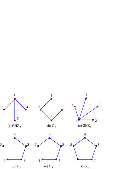
In this paper, we solve the problem of characterizing genuine multiparticle entanglement for certain families of graph-diagonal states, cf. Fig. 1. Graph states are multi-qubit states which are extremely important for many aspects of quantum computation including quantum error correction hein . Graph-diagonal states are states which are diagonal in the associated basis of this graph. Interest in this type of states is physically motivated: they occur naturally upon the decoherence of pure graph states graphdiagonal , and, more importantly, any state can be brought into graph-diagonal form by local operations graphdiagonal ; graphdiagonal2 . As local operations do not affect entanglement properties, this means that if the corresponding graph-diagonal state is entangled the original state was entangled. Thus, entanglement criteria for graph-diagonal states produce entanglement criteria for general states. We note that a widely discussed subset of graph-diagonal states are Greenberger-Horne-Zeilinger-diagonal (GHZ diagonal) states. For these states the characterization of genuine multiparticle entanglement has already been solved seevinck .

Figure 1: The graphs of the states discussed in this paper. (a) and (c): star graphs corresponding to GHZ states. For GHZ-diagonal states with an arbitrary number of qubits, the problem of detecting multiparticle entanglement was already solved in Ref. seevinck . (b) The graph of the four-qubit cluster state. Theorem 3 gives a necessary and sufficient criterion for multipartite entanglement in states which are diagonal in the corresponding graph-state basis. (d,e,f): five-qubit graph states $|Y_{5}\rangle,|C_{5}\rangle,|R_{5}\rangle$. In section IV we determine the border of separability when the graph diagonal generalizations of these states are mixed with white noise. For graph-diagonal states corresponding to the $Y_{5}$-graph, we also obtain a complete characterization of multiparticle entanglement (Theorem 10), which can be generalized to an arbitrary number of qubits (Theorem 12).

This paper is organized as follows: in Section II we introduce the relevant notions of multiparticle entanglement and provide the definition and main properties of graph states. In Section III we specifically consider the four-qubit cluster state and states diagonal in the corresponding basis. We provide a necessary and sufficient criterion for genuine multiparticle entanglement, and, for states without multiparticle entanglement, we provide an explicit decomposition into biseparable states. In Section IV we discuss separability conditions for all five-qubit graph states mixed with white noise. Again, we provide necessary and sufficient criteria for these families and explicit decompositions when the states are separable.

In Section V we relate our results to a recent approach to characterize multiparticle entanglement via so-called positive partial-transpose (PPT) mixtures bastian . Our result for the four-qubit cluster state implies that this criterion is necessary and sufficient for the four-qubit case. The question arises whether this is true in general. We argue that this may not be the case. Nevertheless, in Section VI we discuss in detail the five-qubit Y-shaped graph state for which we can prove that the method of PPT mixtures does deliver a complete solution. In Section VII we discuss generalizations of the Y-shaped graph to an arbitrary number of qubits. Our conclusions and a discussion of possible extensions of our work is presented in Section VIII.

II Multiparticle entanglement and graph states

In this section, we will review the basic notions of genuine multipartite entanglement and graph states. Detailed presentations may be found in Refs. hororeview ; gtreview ; hein and a reader familiar with these topics may skip to the next section.

Let us start with the relevant definitions of multiparticle entanglement for three particles. The generalization to more particles is straightforward. A pure state is called fully separable, if it can be written in the form $|\psi^{\rm fs}\rangle=|a\rangle\otimes|b\rangle\otimes|c\rangle$. A mixed state is fully separable if it can be written as a convex combination of such fully separable pure states, $\varrho^{\rm fs}=\sum_{k}p_{k}|\psi^{\rm fs}_{k}\rangle\langle\psi^{\rm fs}_{k}|,$ where the coefficients $p_{k}$ form a probability distribution, i.e., $p_{k}\geq 0$ and $\sum_{k}p_{k}=1.$

A pure state is called biseparable if it is separable for some bipartition. For example, the state $|\psi^{\rm bs}\rangle=|a\rangle\otimes|\phi^{bc}\rangle$ where $|\phi^{bc}\rangle$ is a possibly entangled state of particles $B$ and $C$ is biseparable for the $A|BC$-partition. Other bipartitions for three particles are the $B|AC$- or $C|AB$-partition. A mixed state is biseparable if it can be written as a sum of biseparable states:

$$\varrho^{\rm bs}=\sum_{k}p_{k}|\psi^{\rm bs}_{k}\rangle\langle\psi^{\rm bs}_{k}|.$$ (1)

Note that the states $|\psi^{\rm bs}_{k}\rangle$ may be biseparable for different partitions. A state is genuine multipartite entangled if it is not biseparable. Genuine multiparticle entanglement is typically the type of entanglement one aims for in experiments gtreview . Consequently, many aspect of multparticle entanglement are under intensive research seevinck ; huber ; bastian . It is the aim of this paper to derive necessary and sufficient conditions of genuine multipartite entanglement for certain families of mixed states known as graph-diagonal states.

Graph states are multi-qubit states defined as follows hein . Let $G$ be a graph: a set of $N$ vertices corresponding to qubits with edges connecting them. Some examples of graphs are shown in Fig. 1. For each vertex $i$, its neighbourhood $\mathcal{N}(i)$ is the set of vertices connected to $i$ by an edge. To define a graph state we associate a stabilizing operator $g_{i}$ to each vertex $i$:

$$g_{i}:=X^{(i)}\bigotimes\nolimits_{j\in\mathcal{N}(i)}Z^{(j)},$$ (2)

where $X^{(i)},Y^{(i)},Z^{(i)}$ denote the Pauli matrices $\sigma_{x},\sigma_{y},\sigma_{z},$ acting on the $i$-th qubit and the identity operator on the rest of the qubits. The qubit index ${(i)}$ may be omitted whenever there is no risk of confusion. The graph state $|G\rangle$ associated with the graph $G$ is the unique $N$-qubit state fulfilling

$$g_{i}|G\rangle=|G\rangle,\mbox{ for }i=1,...,N.$$ (3)

Hence, it is the unique $+1$ eigenstate to all stabilizing operators. Well known examples for graph states are the GHZ states which correspond to the star shaped graphs in Figs. 1(a) and 1(c).

Alternatively, the graph describes a possible construction method of the graph state. Starting with each qubit in the state $|x^{+}\rangle=(|0\rangle+|1\rangle)/\sqrt{2}$ one applies controlled phase-gates to all connected qubits. This results is the graph state $|G\rangle.$ Note that the order in which the phase gates are applied is irrelevant since the controlled phase-gates commute. The construction method for graph states implies, for instance, that the five-qubit linear cluster state [Fig. 1(e)] can be viewed as originating from a four-qubit cluster state [Fig. 1(b)] with an added fifth qubit. We will use this property to prove separability of certain mixed states as follows: if one has a state associated to the four-qubit cluster state which is known to be separable with respect to some partition (say, $AB|CD$ or $12|34$, for definiteness), then the state where the fifth qubit is added [as in Fig. 1(e)] is still separable with respect to the $AB|CDE$ partition.

The definition of a graph state can be extended to different eigenvalues of $g_{i}$ and one may consider all the $2^{N}$ possible states $|\Gamma_{k}\rangle$ where $g_{i}|\Gamma_{k}\rangle=a^{(i)}_{k}|\Gamma_{k}\rangle$ with eigenvalues $a^{(i)}_{k}=\pm 1.$ These vectors are all orthogonal and form the so-called graph state basis for the Hilbert space of $N$ qubits. The $|\Gamma_{k}\rangle$ are uniquely characterized by the $a^{(i)}_{k}$, so one may also write $|\Gamma_{k}\rangle=|a^{(1)}_{k},a^{(2)}_{k},...\rangle$. One can express any of the states as $|\Gamma_{k}\rangle$:

$$|\Gamma_{k}\rangle\langle\Gamma_{k}|=\frac{1}{2^{N}}\prod_{i=1}^{N}(\openone+a^{(i)}_{k}g_{k}),$$ (4)

which will prove useful for our calculations.

In this paper, we focus on graph-diagonal states of the form

$$\varrho=\sum_{k}\lambda_{k}|\Gamma_{k}\rangle\langle\Gamma_{k}|,$$ (5)

where the parameters $\lambda_{k}$ form a probability distribution. This family of states not only has nice mathematical properties but is important for physical reasons as well. An arbitrary $N$-qubit state $\tilde{}\varrho$ can always be brought into a graph-diagonal form by local operations. Moreover, this so-called depolarization map does not change the fidelities $\lambda_{k}=\langle\Gamma_{k}|\tilde{}\varrho|\Gamma_{k}\rangle$ of the graph-basis states. Hence, if the associated graph-diagonal state is entangled then the original $\tilde{}\varrho$ was entangled as well. For experiments, one can measure all the fidelities of the graph states and consider the corresponding graph-diagonal state. Consequently, studying graph-diagonal states has direct consequences for general states, and many properties of graph-diagonal states have been studied in the past few years graphdiagonal ; graphdiagonal2 .

For our later discussion, we note that different graphs may lead to graph states which only differ by a local unitary transformation, implying that their entanglement properties are equivalent. The main graph transformation which leaves the entanglement properties invariant is the so-called local complementation. Local complementation acts on a graph as follows: for a vertex $i$ invert its neighbourhood $\mathcal{N}(i)$. This means that vertices in the neighbourhood that were connected become disconnected and vice versa. For example, local complementation on qubit 1 of graph in Fig. 1(a) will transform it into a graph that is fully connected. Similarly, local complementation of qubit 2 in Fig. 1(b) will connect qubits 1 and 3. Modulo local complementation, there are only two independent four-qubit graphs and four five-qubit graphs all of which are displayed in Fig. 1.

As an example of a graph state, let us consider the graph in Fig. 1(b). The stabilizing operators of this graph are

$$g_{1}=XZ11,\;\;g_{2}=ZXZ1,\;\;g_{3}=1ZXZ,\;\;g_{4}=11ZX,$$ (6)

and the associated graph state is the so-called cluster state $|C_{4}\rangle.$ After a local transformation, the cluster state can also be written in the common representation hein

$$|C_{4}^{\prime}\rangle=\frac{1}{2}(|0000\rangle+|0011\rangle+|1100\rangle-|1111\rangle),$$ (7)

given in the computational basis. We will work, however, in the basis defined by the stabilizers in Eq. (6). The cluster state $|C_{4}\rangle$ is an eigenstate of the $g_{i}$ with $+1$ eigenvalue. As indicated above, we can write $|C_{4}\rangle$ as $|\!+\!+\!+\!+\rangle$, where the qubits are written in the order $ABCD$. Similarly, the other states in the basis can be denoted by $|\!+\!+\!+\!-\rangle,...,|\!-\!-\!-\!-\rangle$. We write these states in general as $|ijkl\rangle$ with $i,j,k,l\in\{+,-\}.$ When using this notation, we denote with $\bar{i},\bar{j},\bar{k},\bar{l}$ the opposite signs to $i,j,k,l$; such that $i\bar{i}=-1$ etc. We also find it convenient to abbreviate projectors as $|ijkl\rangle\langle\cdot|\equiv|ijkl\rangle\langle ijkl|.$ Finally, let us recall that the signs of all the states in the graph state basis can be changed by applying the Pauli matrix $Z$ to the corresponding qubits. As these are local operations they do not change the states’ entanglement properties.

III Cluster-diagonal states of four qubits

In this section, we will derive a necessary and sufficient criterion for the presence of genuine multipartite entanglement in cluster-diagonal states of four qubits. Before proving our main result, we need two lemmata. The first one characterizes a set of entanglement witnesses for genuine multipartite entanglement, while the second one identifies a large class of biseparable quantum states that will simplify the search for biseparable decompositions.

Lemma 1. The observables

$$\mathcal{W}_{1} = \frac{\openone}{2}-|C_{4}\rangle\langle C_{4}|-\frac{1}{2}\frac{\openone-g_{1}}{2}\frac{\openone-g_{4}}{2}$$

$$= \frac{\openone}{2}-|\!+\!+\!+\!+\rangle\langle\cdot|-\frac{1}{2}\sum_{ij}|\!-ij-\rangle\langle\cdot|,$$

$$\mathcal{W}_{2} = \frac{\openone}{2}-|\!+\!+\!+\!+\rangle\langle\cdot|-|\!-\alpha\beta-\rangle\langle\cdot|,$$ (8)

are entanglement witnesses for genuine multipartite entanglement. That is, ${\rm Tr}(\varrho\mathcal{W}_{k})<0$ implies the presence of genuine multipartite entanglement in $\varrho.$ This holds for arbitrary signs $\alpha,\beta$ in $\mathcal{W}_{2}.$

Proof. It was proven in Ref. bastian that $\mathcal{W}_{1}$ is a witness. The fact that $\mathcal{W}_{2}$ is a witness can be demonstrated in a similar way. It suffices to show that $(\mathcal{W}_{2})^{T_{M}}\geq 0$ for all possible bipartitions $M.$ The operators $(\mathcal{W}_{2})^{T_{M}}$ are diagonal in the graph state basis. Thus, it is enough to show that $\langle ijkl|(\mathcal{W}_{2})^{T_{M}}|ijkl\rangle\geq 0$ holds for all elements of the graph state basis. This, however, is a direct consequence of Lemma 2 and Lemma 3 in the Appendix of Ref. bastian . ∎

Lemma 2. The quantum states

$$\sigma=\frac{1}{2}(|ijkl\rangle\langle\cdot|+|\alpha\beta\gamma\delta\rangle\langle\cdot|)$$ (9)

are biseparable, unless $i\neq\alpha$ and $l\neq\delta$ both hold at the same time.

Proof. First, we note that if $i\neq\alpha$ and $l\neq\delta$ the state is definitely not biseparable, since it is detected by a witness of the type $\mathcal{W}_{2}$ (and also by $\mathcal{W}_{1}$). Now, we show explicitly that all other states are biseparable. We can assume without loss of generality that $|ijkl\rangle=|\!+\!+\!+\!+\rangle$ since any $|ijkl\rangle$ can be transformed into $|\!+\!+\!+\!+\rangle$ by local transformations and we neglect the normalization of $\sigma$. The first example is presented in great detail so as to demonstrate our methodology.

(a) Consider the state $\sigma=|\!+\!+\!++\rangle\langle\cdot|+|\!-\!+\!++\rangle\langle\cdot|.$ There are two ways to see that $\sigma$ is biseparable with respect to the $A|BCD$ partition and we will discuss both of them, in order to illustrate the different methods.

(a1) The first method starts with the fact that for two qubits any mixture of two Bell states with equal weight (e.g., $\eta=|\Phi^{+}\rangle\langle\Phi^{+}|+|\Phi^{-}\rangle\langle\Phi^{-}|$) is separable horoalt . The graph corresponding to a Bell state is the connected two-qubit graph. The four-qubit state $\sigma$ can be considered as a separable mixture of the two Bell states $|\!++\rangle\langle\cdot|+|\!-+\rangle\langle\cdot|$ on the first two qubits $AB$, where the qubits $CD$ have been subsequently added to $B$ via some local interaction. Clearly, the state $\sigma$ remains biseparable between $A$ and the rest of the qubits.

(a2) The second method uses Eq. (4) to write

$$\sigma \sim(\openone+g_{2})(\openone+g_{3})(\openone+g_{4})$$

$$\sim(\openone+ZXZ1)(\openone+1ZXZ)(\openone+11ZX)$$

$$\sim\underbrace{(\openone+Z111)}_{\sim|0\rangle\langle 0|}\underbrace{(\openone+g_{2}^{\rm red})(\openone+g_{3})(\openone+g_{4})}_{\rm stabilizer\;\;state\;\;on\;\;qubits\;\;2,3,4}$$

$$+\underbrace{(\openone-Z111)}_{\sim|1\rangle\langle 1|}\underbrace{(\openone-g_{2}^{\rm red})(\openone+g_{3})(\openone+g_{4})}_{\rm stabilizer\;\;state\;\;on\;\;qubits\;\;2,3,4},$$ (10)

where $g_{2}^{\rm red}=1XZ1$ denotes the restriction of the stabilizer $g_{2}$ to the qubits 2,3,4. In this form the state is clearly biseparable, since it is written as a sum of two terms, which are both biseparable with respect to the $A|BCD$-partition. This rewriting is possible, since in the expansion $\sigma\sim(\openone+g_{2})(\openone+g_{3})(\openone+g_{4})$ only the identity and one of the Pauli matrices (here: $Z$) occur on the first qubit, cf. Eq. (III). This statement holds for any Pauli operator. With these two methods in hand we now prove the other states, $\sigma$, are also biseparable.

(b) We consider $\sigma=|\!+\!+\!+\!+\rangle\langle\cdot|+|\!+\!-\!+\!+\rangle\langle\cdot|.$ Using (a1) this is clearly separable with respect to the $A|BCD$ partition, but it is also separable with respect to the $B|ACD$-partition, as can be seen using the idea of (a2).

(c) The state $\sigma=|\!+\!+\!+\!+\rangle\langle\cdot|+|\!-\!-\!+\!+\rangle\langle\cdot|$ is biseparable with respect to the $A|BCD$-partition according to (a1).

(d) The state $\sigma=|\!+\!+\!+\!+\rangle\langle\cdot|+|\!-\!+\!-\!+\rangle\langle\cdot|\sim(\openone+g_{1}g_{3})(\openone+g_{2})(\openone+g_{4})$ is biseparable with respect to the $B|ACD$ partition, as can be seen using (a2).

(e) The state $\sigma=|\!+\!+\!+\!+\rangle\langle\cdot|+|\!+\!-\!-\!+\rangle\langle\cdot|$ can be shown to be biseparable using the method of (a1) with qubits $B$ and $C$ as the Bell pair. Consequently, it is separable with respect to the $AB|CD$-partition.

(f) Finally, we consider $\sigma=|\!+\!+\!+\!+\rangle\langle\cdot|+|\!-\!-\!-\!+\rangle\langle\cdot|\sim(\openone+g_{1}g_{2}+g_{2}g_{3}+g_{1}g_{3})(\openone+g_{4}).$ First, using the method of (a2) one can directly calculate that this state is separable with respect to the $B|ACD$-partition. However, one can also apply the method of (a1): On the first three qubits, one can consider the state $\sigma=|\!+\!++\rangle\langle\cdot|+|\!-\!--\rangle\langle\cdot|.$ This corresponds to a mixture of two three-qubit GHZ states, and it is known that such mixtures are always biseparable seevinck . For $\sigma$ only one qubit is added similar to (a1), so $\sigma$ has to be biseparable, too. Up to symmetries these are all the relevant cases. ∎

We can now formulate and prove our main result. We denote the fidelities of the graph basis states as $F_{++++}=\langle\!+\!+\!+\!+|\varrho|\!+\!+\!+\!+\rangle$ etc. We can then state:

Theorem 3. A cluster-diagonal four-qubit state $\varrho$ is biseparable, if and only if for all indices $\alpha,\beta,\gamma,\delta$

$$2 F_{\alpha\beta\gamma\delta}\leq\sum_{i,j}F_{\alpha ij\delta}+\sum_{i,j}F_{\bar{\alpha}ij\delta}+\sum_{i,j}F_{\alpha ij\bar{\delta}}$$ (11)

holds and for all indices $\alpha,\beta,\gamma,\delta,\mu,\nu$ the inequalities

$$2F_{\alpha\beta\gamma\delta}+2F_{\bar{\alpha}\mu\nu\bar{\delta}}\leq \sum_{i,j}F_{\alpha ij\delta}+\sum_{i,j}F_{\bar{\alpha}ij\delta}$$

$$+\sum_{i,j}F_{\alpha ij\bar{\delta}}+\sum_{i,j}F_{\bar{\alpha}ij\bar{\delta}}$$ (12)

are satisfied.

Before proving this result, let us interpret the conditions in Eqs. (11, 12). In light of Lemma 2, Eq. (11) compares the weight of the state $|\alpha\beta\gamma\delta\rangle\langle\cdot|$ with the sum of the weights of all other states, which can be used to build a biseparable pair with $|\alpha\beta\gamma\delta\rangle\langle\cdot|$. If the overall state is biseparable the first weight has to be smaller than the other weights, otherwise a decomposition with the methods of Lemma 2 cannot be found. The condition Eq. (12) then compares the weights of two states, $|\alpha\beta\gamma\delta\rangle\langle\cdot|$ and $|\bar{\alpha}\beta\gamma\bar{\delta}\rangle\langle\cdot|$ (which, according to Lemma 2, do not constitute a separable pair) with all other weights. Using the normalization of the state, Eq. (12) can be rephrased as $F_{\alpha\beta\gamma\delta}+F_{\bar{\alpha}\mu\nu\bar{\delta}}\leq 1/2$, which has a natural meaning: if the weight of one “inseparable” pair exceeds all other weights, then the state cannot be separable.

Proof. We will use a shorthand notation for the sums such that Eq. (11), $2F_{++++}\leq\sum_{ij}F_{+ij+}+\sum_{ij}F_{-ij+}+\sum_{ij}F_{+ij-}$, is abbreviated as $2F_{++++}\leq\sum_{++}+\sum_{-+}+\sum_{+-}.$

We first have to show that if one of the conditions in Eqs. (11, 12) is violated, then $\varrho$ is genuinely multipartite entangled. This follows directly from Lemma 1 since the conditions (11, 12) are nothing but a rewriting of ${\rm Tr}(\mathcal{W}_{k}\varrho)\geq 0.$

It remains to show that a state is biseparable, if Eqs. (11, 12) hold. Clearly, this is the difficult part. Our proof is split into four cases:

Case 1 — Let us first assume that the state $\varrho$ acts only on the four-dimensional space spanned by the vectors $|\!-\!ij-\rangle$ and that the relevant four fidelities fulfill $F_{-\alpha\beta-}\leq F_{-\alpha\bar{\beta}-}+F_{-\bar{\alpha}\beta-}+F_{-\bar{\alpha}\bar{\beta}-}$ for all $\alpha,\beta$. Then, the state $\varrho$ is separable with respect to the $AB|CD$ partition. The reason is the following: a mixture of two-qubit Bell states, $\sigma=\lambda_{++}|\Phi^{+}\rangle\langle\Phi^{+}|+\lambda_{+-}|\Phi^{-}\rangle\langle\Phi^{-}|+\lambda_{-+}|\Psi^{+}\rangle\langle\Psi^{+}|+\lambda_{--}|\Psi^{-}\rangle\langle\Psi^{-}|$, is easily seen to be separable iff $\lambda_{\alpha\beta}\leq\lambda_{\alpha\bar{\beta}}+\lambda_{\bar{\alpha}\beta}+\lambda_{\bar{\alpha}\bar{\beta}}$ for all $\alpha,\beta$ horoalt . The four-qubit state $\varrho$ is nothing but a mixture of such Bell states between $B$ and $C$, with qubits $A$ and $D$ added [see also case (a1) in the proof of Lemma 2].

Case 2 — Now we assume that equality holds for one of the conditions of Eq. (11). Without loss of generality, we assume that $2F_{++++}=\sum_{++}+\sum_{+-}+\sum_{-+}$ while the other conditions in Eqs. (11, 12) are fulfilled, but not necessarily with equality.

In this case, Eq. (12) becomes $F_{-\alpha\beta-}\leq F_{-\alpha\bar{\beta}-}+F_{-\bar{\alpha}\beta-}+F_{-\bar{\alpha}\bar{\beta}-}$, the same relation discussed in Case 1. If we consider now the projection $\varrho^{\rm R}$ of the original state $\varrho$ on the four-dimensional space spanned by the vectors $|\!-\!ij-\rangle,$ then it is clear that this state $\varrho^{\rm R}$ is separable according to Case 1. It remains to show that the orthogonal part $\varrho-\varrho^{\rm R}$ is separable too. For this part we have $F_{++++}=F_{+--+}+F_{++-+}+F_{+-++}+\sum_{+-}+\sum_{-+,}$ so it can be directly decomposed with the help of Lemma 2, by using all possible combinations of the type $|\!+\!+\!++\rangle\langle\cdot|+|\alpha\beta\gamma\delta\rangle\langle\cdot|$. This finishes the proof of Case 2.

Case 3 — In this case we assume that equality holds for one of the conditions of Eq. (12): $2F_{++++}+2F_{----}=\sum_{++}+\sum_{+-}+\sum_{-+}+\sum_{--}.$ The other inequalities in Eqs. (11, 12) are satisfied, but not necessarily with equality. Rewriting, gives us $(2F_{++++}-\sum_{++})+(2F_{----}-\sum_{--})=\sum_{+-}+\sum_{-+}.$ Using this together with the inequalities given by Eq. (11) we can also deduce the conditions $2F_{----}\geq\sum_{--}$ and $2F_{++++}\geq\sum_{++}$.

Now, we can decompose $\varrho$ as follows: Consider the space spanned by $|\!-\!ij-\rangle,$ and a state $\sigma^{-}$ with $F^{\prime}_{----}:=\sum_{--}-F_{----}=F_{--+-}+F_{-+--}+F_{-++-}$ and $F^{\prime}_{-ij-}:=F_{-ij-}$ otherwise. This state is separable according to Case 1, since $F^{\prime}_{----}=F^{\prime}_{--+-}+F^{\prime}_{-+--}+F^{\prime}_{-++-}$. The restriction $\varrho^{\rm R}$ of $\varrho$ onto the four-dimensional subspace is now given by $\varrho^{\rm R}=\sigma^{-}+(F_{----}-F^{\prime}_{----})\linebreak|\!-\!-\!--\rangle\langle\cdot|=\sigma^{-}+(2F_{----}-\sum_{--})|\!-\!-\!--\rangle\langle\cdot|.$ We can make a similar construction on the space spanned by $|\!+\!ij+\rangle$ with a separable state $\sigma^{+}$. A projector onto $|\!+\!+\!+\!+\rangle$ with weight $(2F_{++++}-\sum_{++})$ will remain.

Therefore, we can decompose $\varrho$ into the two separable states $\sigma^{-}$ and $\sigma^{+}$ on the four-dimensional spaces and a remaining state $\eta.$ The state $\eta$ has only two contributions on the two four-dimensional spaces, which have the fidelities $F_{++++}^{\eta}=2F_{++++}-\sum_{++}$ and $F_{----}^{\eta}=2F_{----}-\sum_{--}.$ From our assumption, it follows that $\eta$ fulfils $F_{++++}^{\eta}+F_{----}^{\eta}=\sum_{+-}+\sum_{-+}$. This remaining state $\eta$ can then be decomposed using states of the form $\sigma=|\!-\!-\!-\!-\rangle\langle\cdot|+|\!-\!kl+\rangle\langle\cdot|$ and $\sigma=|\!-\!-\!-\!-\rangle\langle\cdot|+|\!+\!kl-\rangle\langle\cdot|$ etc.

Case 4 — Let us finally discuss the case where equality holds for none of the conditions of Eqs. (11, 12). We consider the state

$$\varrho^{\rm new}=\varrho-\varepsilon\sigma,$$ (13)

where $\sigma$ is one of the separable states from Lemma 2. Since $\varrho=\varrho^{\rm new}+\varepsilon\sigma$ the state $\varrho$ is separable, if $\varrho^{\rm new}$ is separable and positive.

The idea is to choose possible biseparable states $\sigma$ and subtract them step by step such that $\varrho^{\rm new}$ remains positive. Note that during these subtractions, the inequalities (11, 12) become tighter. But one does not have to worry that they become violated: If they become violated, at some point equality must hold in one of the two Eqs. (11,12) first, while the other conditions still hold. This means that at this point $\varrho^{\rm new}$ (and hence $\varrho$) is separable, according to Cases 2 and 3.

What can be achieved with the iterative subtractions? First, by subtracting the biseparable states $\sigma=|\!+\!ij+\rangle\langle\cdot|+|\!+\!kl+\rangle\langle\cdot|$ one can set three of the $F_{+\alpha\beta+}$ to zero. Similarly, in each of the sets $\{F_{+\alpha\beta-}\}$, $\{F_{-\alpha\beta+}\}$ and $\{F_{-\alpha\beta-}\}$ three fidelities can be made to vanish, such that overall only four $F_{ijkl}$ are nonzero. The structure of the fidelities is now such that all the sums in Eqs. (11, 12) contain only a single term. Then, however, Eq. (12) must either be violated for some set of indices, or equality must hold. ∎

Using this theorem we can determine that cluster states mixed with white noise, $\varrho(p)=p|C_{4}\rangle\langle C_{4}|+(1-p){\openone}/{16}$, are entangled iff $p>5/13.$ This confirms a numerically established threshold from Ref. bastian .

Furthermore, the theorem demonstrates that for cluster-diagonal states there are effectively only two entanglement witnesses, namely the ones from Lemma 1. It is interesting to compare this with the results of Ref. seevinck , where a necessary and sufficient criterion for GHZ diagonal states was found. This criterion can be interpreted in the sense that for GHZ diagonal states (of an arbitrary number of qubits) only one entanglement witness is relevant, namely $\mathcal{W}=\openone/2-|GHZ_{N}\rangle\langle GHZ_{N}|.$ For cluster states, the witness $\mathcal{W}=\openone/2-|C_{4}\rangle\langle C_{4}|$ is not optimal, since both of the witnesses in Lemma 1 are better. One can expect that for more complicated graph states of more qubits, a significant higher number of witnesses is relevant, hence a complete classification becomes difficult.

IV Five-qubit graph states

In this section, we derive optimal criteria for all five-qubit graph states mixed with white noise. Doing this demonstrates that the witnesses obtained with the PPT approach of Refs. bastian ; bastian2 are optimal. In the next section, however, we will argue that the success of the PPT approach in finding optimal witnesses might be specific to these states. Nevertheless, we do present full solution of the cluster state $Y_{5}$ in Section VI, cf. Theorem 10.

IV.1 The state $Y_{5}$

For the five-qubit $Y_{5}$ state [see Fig. 1(d)] mixed with white noise we demonstrate:

Proposition 4. The state

$$\varrho(p)=p|Y_{5}\rangle\langle Y_{5}|+(1-p)\frac{\openone}{32}$$ (14)

is genuine multipartite entangled if and only if $p>9/25=0.36.$

Proof. First, for the case that $p>9/25$ the state $\varrho(p)$ is detected by the witness bastian2

$$\mathcal{W}_{Y5}=\frac{\openone}{2}-|Y_{5}\rangle\langle Y_{5}|-\frac{1}{16}\big{[}(\openone-g_{1})(\openone-g_{4})(\openone+g_{5})$$

$$+(\openone-g_{1})(\openone+g_{4})(\openone-g_{5})+(\openone-g_{1})(\openone-g_{4})(\openone-g_{5})\big{]}$$ (15)

and, hence, genuine multipartite entangled.

In the other direction, we first have to identify the separable states as we did in Lemma 2. In fact, for many states this lemma can be directly generalized. For instance, the state $\sigma=|\!+\!+\!+\!++\rangle\langle\cdot|+|ijk\!++\rangle\langle\cdot|$ is biseparable, since for the four-qubit cluster state $\sigma^{\prime}=|\!+\!+\!+\!+\rangle\langle\cdot|+|ijk+\rangle\langle\cdot|$ is separable, and the fifth qubit is added as in case (a1) in the proof of Lemma 2. In fact, the only combinations which are not separable are of the form $\chi_{1}=|\!+\!+\!+\!++\rangle\langle\cdot|+|\!-\!jk\!-+\rangle\langle\cdot|$ and $\chi_{2}=|\!+\!+\!+\!++\rangle\langle\cdot|+|\!-\!jkl\!-\rangle\langle\cdot|$. Note that the state $\sigma=|\!+\!+\!+\!++\rangle\langle\cdot|+|+jk\!-\!-\rangle\langle\cdot|$ is biseparable, because it can be considered as a separable four-qubit GHZ state on BCDE where one qubit is added [see case (f) in the proof of Lemma 2].

The state at the critical value of $p$ is

$$\varrho\sim 19|\!+\!+\!+\!++\rangle\langle\cdot|+\sum_{ijklm\neq+++++}|ijklm\rangle\langle\cdot|,$$ (16)

and it remains to show that this state is separable. First, the state

$$\varrho^{\prime}=19|\!+\!+\!+\!++\rangle\langle\cdot|+\big{[}\sum_{ijklm\neq+++++}|ijklm\rangle\langle\cdot|$$

$$-\sum_{ij}|\!-\!ij\!-\!+\rangle\langle\cdot|-\sum_{ij}|\!-\!ij\!+\!-\rangle\langle\cdot|-\sum_{ij}|\!-\!ij\!-\!-\rangle\langle\cdot|\big{]}$$ (17)

is biseparable, since in the sums in the brackets exactly 19 terms remain, and a decomposition with $\sigma$ from above is then straightforward. The remaining term $\varrho-\varrho^{\prime}=\sum_{ij}|\!-\!ij\!-\!+\rangle\langle\cdot|+\sum_{ij}|\!-\!ij\!+\!-\rangle\langle\cdot|+\sum_{ij}|\!-\!ij\!-\!-\rangle\langle\cdot|$ is also clearly separable, since the sum of any two of the occurring states is separable. ∎

IV.2 The linear cluster state $C_{5}$

For the five-qubit linear cluster $C_{5}$ state [see Fig. 1(e)] mixed with white noise the threshold is the same as for the $Y_{5}$ state:

Proposition 5. The state

$$\varrho(p)=p|C_{5}\rangle\langle C_{5}|+(1-p)\frac{\openone}{32}$$ (18)

is genuine multipartite entangled if and only if $p>9/25=0.36.$

Proof. First, the witness

$$\mathcal{W}_{C5}=\frac{\openone}{2}-|C_{5}\rangle\langle C_{5}|-\frac{1}{32}\big{[}4(\openone-g_{1})(\openone-g_{5})$$

$$+(\openone+g_{1})(\openone-g_{2})(\openone-g_{5})+(\openone-g_{1})(\openone-g_{4})(\openone+g_{5})\big{]}$$ (19)

detects the state for $p>9/25,$ proving one part of the claim bastian2 .

For the other direction, we have to again identify the biseparable states. First, in a generalization of Lemma 2, states of the form $\sigma=|\!+\!+\!+\!++\rangle\langle\cdot|+|ijklm\rangle\langle\cdot|$ are separable, unless they are of the form $\chi_{1}=|\!+\!+\!+\!++\rangle\langle\cdot|+|\!-\!jk\!-+\rangle\langle\cdot|,$ $\chi_{2}=|\!+\!+\!+\!++\rangle\langle\cdot|+|\!+\!-\!jk-\rangle\langle\cdot|,$ or $\chi_{3}=|\!+\!+\!+\!++\rangle\langle\cdot|+|\!-\!jkl-\rangle\langle\cdot|.$ There are 16 terms of this type which are not biseparable.

The state at $p=9/25$ is, up to normalization, given by $\varrho=19|\!+\!+\!+\!++\rangle\langle\cdot|+\sum_{ijklm\neq+++++}|ijklm\rangle\langle\cdot|.$ Generalizing Lemma 2 we can subtract many pairs of terms such that what remain is to show that

$$\varrho^{\prime}= 4|\!+\!+\!+\!++\rangle\langle\cdot|+\sum_{ij}|\!-ij-\!+\rangle\langle\cdot|$$

$$+\sum_{ij}|\!+\!-ij-\rangle\langle\cdot|+\sum_{ijk}|\!-\!ijk-\rangle\langle\cdot|$$ (20)

is separable. To do this let us consider the four states

$$\eta_{1} = |\!+\!+\!+\!++\rangle\langle\cdot|+|\!+\!-\!+\!+-\rangle\langle\cdot|+|\!-\!+\!+\!-+\rangle\langle\cdot|$$

$$+|\!-\!-\!+\!--\rangle\langle\cdot|,$$

$$\eta_{2} = |\!+\!+\!+\!++\rangle\langle\cdot|+|\!+\!-\!+\!--\rangle\langle\cdot|+|\!-\!-\!+\!-+\rangle\langle\cdot|$$

$$+|\!-\!+\!+\!+-\rangle\langle\cdot|,$$

$$\eta_{3} = |\!+\!+\!+\!++\rangle\langle\cdot|+|\!+\!-\!-\!+-\rangle\langle\cdot|+|\!-\!-\!-\!-+\rangle\langle\cdot|$$

$$+|\!-\!+\!+\!--\rangle\langle\cdot|,$$

$$\eta_{4} = |\!+\!+\!+\!++\rangle\langle\cdot|+|\!+\!-\!-\!--\rangle\langle\cdot|+|\!-\!+\!-\!-+\rangle\langle\cdot|$$ (21)

$$+|\!-\!-\!+\!+-\rangle\langle\cdot|.$$

The state $\eta_{1}$ is separable for the following reason: it is known that the four-qubit Smolin state $\sigma=|\Phi^{+}\rangle\langle\Phi^{+}|_{AB}\otimes|\Phi^{+}\rangle\langle\Phi^{+}|_{A^{\prime}B^{\prime}}+|\Phi^{-}\rangle\langle\Phi^{-}|_{AB}\otimes|\Phi^{-}\rangle\langle\Phi^{-}|_{A^{\prime}B^{\prime}}+|\Psi^{+}\rangle\langle\Psi^{+}|_{AB}\otimes|\Psi^{+}\rangle\langle\Psi^{+}|_{A^{\prime}B^{\prime}}+|\Psi^{-}\rangle\langle\Psi^{-}|_{AB}\otimes|\Psi^{-}\rangle\langle\Psi^{-}|_{A^{\prime}B^{\prime}}$ is separable with respect to the $AA^{\prime}|BB^{\prime}$ partition smolin . The state $\eta_{1}$ is simply a Smolin state between the qubits $ABDE$, where the qubit $C$ has been added [see case (a1) in Lemma 2]. Therefore, it is separable with respect to the $AE|BCD$-partition. Similarly, $\eta_{2}$ is a Smolin state up to local unitary operations and therefore separable with respect to the same partition.

It can be directly verified that the state $\eta_{3}$ is PPT with respect to the $BD|ACE$ partition. This implies separability via the following argument: for the considered partition, $\eta_{3}$ is acting on a $4\times 8$ (effectively $4\times 4$) space. The PPT entangled states in this scenario have at least a rank of five horobounddim . Hence, $\eta_{3}$, which is of rank four, must be separable with respect to the partition . Similarly, $\eta_{4}$ is separable with respect to the $BD|ACE$-partition.

So we can write

$$\varrho^{\prime}=\sum_{k=1}^{4}\eta_{k}+\sum_{ij}|\!-\!i\!-\!j-\rangle\langle\cdot|$$ (22)

where the sum of the remaining four projectors is clearly separable according to Lemma 2. This finishes the proof. ∎

IV.3 The ring cluster state $R_{5}$

For the five-qubit ring cluster state mixed with white noise the separability problem can be solved as follows:

Proposition 6. The state

$$\varrho(p)=p|R_{5}\rangle\langle R_{5}|+(1-p)\frac{\openone}{32}$$ (23)

is genuine multipartite entangled if and only if $p>7/19\approx 0.368.$

Proof. Due to the symmetry of this state, it is convenient for our discussion to define $\mathcal{T}(x)$ as the sum over all five translations of the term $x$, corresponding to a rotation of the ring graph. The witness for the state is then given in bastian2 :

$$\mathcal{W}_{R5} = 3\times\big{[}\mathcal{T}(|\!+\!+\!+\!+-\rangle\langle\cdot|)+\mathcal{T}(|\!+\!+\!-\!+-\rangle\langle\cdot|)$$ (24)

$$+\mathcal{T}(|\!+\!+\!-\!--\rangle\langle\cdot|)\big{]}$$

$$+ \big{[}\mathcal{T}(|\!+\!+\!+\!--\rangle\langle\cdot|)+\mathcal{T}(|\!+\!-\!+\!--\rangle\langle\cdot|)$$

$$+\mathcal{T}(|\!+\!-\!-\!--\rangle\langle\cdot|)\big{]}$$

$$- |\!-\!-\!-\!--\rangle\langle\cdot|-3\times|\!+\!+\!+\!++\rangle\langle\cdot|.$$

This witness detects the entanglement in the state for $p>7/19$, proving one direction of the claim.

For the other direction, we have to identify separable states. First, states like $\sigma_{1}=|\!+\!+\!+\!++\rangle\langle\cdot|+|\!+\!+\!+\!+-\rangle\langle\cdot|$ $\sigma_{2}=|\!+\!+\!+\!++\rangle\langle\cdot|+|\!+\!+\!-\!+-\rangle\langle\cdot|$ and $\sigma_{3}=|\!+\!+\!+\!++\rangle\langle\cdot|+|\!+\!+\!-\!--\rangle\langle\cdot|$ are clearly separable in analogy to Lemma 2: $\sigma_{1}$ is separable in analogy to case (a2), $\sigma_{2}$ and $\sigma_{3}$ can be considered as states on the qubits $BCDE$ which are separable with respect to the $D|BCE$ partition [cases (d) and (f) in Lemma 2], where the qubit $A$ is added by a local transformation. Furthermore, the states

$$\eta_{1} = |\!+\!+\!+\!++\rangle\langle\cdot|+|\!+\!-\!-\!++\rangle\langle\cdot|+|\!-\!-\!+\!-+\rangle\langle\cdot|$$

$$+|\!-\!+\!-\!-+\rangle\langle\cdot|,$$

$$\eta_{2} = |\!+\!+\!+\!++\rangle\langle\cdot|+|\!-\!-\!+\!++\rangle\langle\cdot|+|\!+\!+\!-\!-+\rangle\langle\cdot|$$

$$+|\!-\!-\!-\!-+\rangle\langle\cdot|,$$

$$\eta_{3} = |\!+\!+\!+\!++\rangle\langle\cdot|+|\!-\!-\!+\!++\rangle\langle\cdot|+|\!-\!+\!-\!--\rangle\langle\cdot|$$

$$+|\!+\!-\!-\!--\rangle\langle\cdot|,$$

$$\eta_{4} = |\!+\!+\!+\!++\rangle\langle\cdot|+|\!-\!-\!+\!-+\rangle\langle\cdot|+|\!+\!-\!-\!+-\rangle\langle\cdot|$$ (25)

$$+|\!-\!+\!-\!--\rangle\langle\cdot|.$$

are also separable. The state $\eta_{1}$ is separable with respect to the $BC|ADE$-partition, as can be seen from the separability properties of the Smolin state (similar to the state $\eta_{1}$ defined for the linear cluster state $C_{5}$ above). $\eta_{2}$ is PPT with respect to the $BC|ADE$-partition, and hence separable (due to a rank argument as in the proof of Proposition 5.). The separability of $\eta_{3}$ (and $\eta_{4}$) can be inferred from their being PPT with respect to the $CE|ABD$ (and $AC|BDE$) partition.

The state at $p=7/19$ is given by $\varrho=59|\!+\!+\!+\!++\rangle\langle\cdot|+3\times\sum_{ijklm\neq+++++}|ijklm\rangle\langle\cdot|$ which can be written as

$$\varrho=3\times\sum_{k=1}^{3}\mathcal{T}(\sigma_{k})+\frac{14}{20}\times\sum_{k=1}^{4}\mathcal{T}(\eta_{k})+\varrho^{\prime}$$ (26)

with

$$\varrho^{\prime} = \frac{1}{5}\mathcal{T}(|\!+\!+\!+\!--\rangle\langle\cdot|)+\frac{1}{5}\mathcal{T}(|\!+\!-\!+\!--\rangle\langle\cdot|)$$ (27)

$$+\frac{1}{5}\mathcal{T}(|\!+\!-\!-\!--\rangle\langle\cdot|)+3|\!-\!-\!-\!--\rangle\langle\cdot|.$$

This state, however, can directly be decomposed in terms of the $\sigma_{k}$ with all signs inverted. ∎

V Connection with the theory of PPT mixtures

In order to place our results within a wider framework, we discuss possible connections with the theory of PPT mixtures, introduced in Refs. bastian ; bastian2 . In these papers, the following approach to characterize multiparticle entanglement has been proposed: instead of considering biseparable states of the form

$$\varrho^{\rm bs}=\sum_{k}p_{k}|\psi^{\rm bs}_{k}\rangle\langle\psi^{\rm bs}_{k}|,$$ (28)

where the states $|\psi^{\rm bs}_{k}\rangle\langle\psi^{\rm bs}_{k}|$ are separable with respect to some partition, consider states of the form

$$\varrho^{\rm pmix}=\sum_{k}p_{k}\varrho^{\rm ppt}_{k},$$ (29)

with states $\varrho^{\rm ppt}_{k}$ that have a positive partial transpose (PPT) with respect to some bipartition. Such states are called PPT mixtures. Since separable states are also PPT, the set of biseparable states is a subset of the set of PPT mixtures. Consequently, proving that a state is not a PPT mixture implies genuine multiparticle entanglement.

The advantage of this approach is that the set of PPT mixtures can be characterized much more easily than the set of biseparable states. For instance, for a small number of (up to seven) qubits one can directly decide whether a state is a PPT mixture via the method of semidefinite programming pptmixture . Moreover, witnesses detecting states that are not PPT mixtures can be derived analytically. This has been done for many types of graph states in Ref. bastian2 .

With respect to the results reported here, it is remarkable that all the witnesses used in this paper [Lemma 1 and Eqs. (15, 19, 24)] were derived from the theory of PPT mixtures. Any PPT mixture within the considered subclass (e.g., the cluster-diagonal states) will therefore fulfill the conditions set by the witnesses [e.g., Eqs. (11, 12)] and must be biseparable. In other words, we have shown that for the families of graph-diagonal states considered here, biseparability is equivalent to being a PPT mixture.

This leads to the question, whether it is generally true that graph-diagonal states are biseparable if and only if they are PPT mixtures. If this conjecture were true, it would solve the problem of characterizing multiparticle entanglement for a huge class of states with an arbitrary number of qubits. Moreover, for graph-diagonal states the problem can be solved with linear programming, which is significantly simpler than semidefinite programming bastian2 and which could deal with larger qubit systems. However, there is evidence that the conjecture is not correct, as we explain in the following.

First, note that when looking for a decomposition of a graph-diagonal state into biseparable (or PPT) states, one can assume that the terms in the decomposition are also graph-diagonal. If one finds a decomposition where this is not the case, one can always apply the local depolarization map explained in Section II between Eqs. (5) and (6) . The graph-diagonal state is invariant, but terms in the decomposition which are not diagonal, become diagonal after application of the map. Since this operation is local, the state remains biseparable or PPT.

Therefore, if any graph-diagonal state which is PPT with respect to a given bipartition, is also separable with respect to the same bipartition, the conjecture would be correct. However, this is not always the case. Examples can be given from bound entangled states known in the literature benatti ; piani . For instance, consider the four-qubit cluster-diagonal state

$$\tilde{\varrho} = \frac{1}{6}(|\!+\!+\!--\rangle\langle\cdot|+|\!-\!+\!+-\rangle\langle\cdot|+|\!-\!-\!-+\rangle\langle\cdot|\phantom{++}$$ (30)

$$+|\!+\!-\!+-\rangle\langle\cdot|+|\!+\!-\!--\rangle\langle\cdot|+|\!+\!-\!-+\rangle\langle\cdot|).$$

where the qubits are as usually written in the order $ABCD.$ Though this state is PPT with respect to the $AD|BC$ partition it is entangled with respect to the same partition. This can be seen as follows: In Ref. benatti the four-qubit state $\hat{\varrho}$

$$\hat{\varrho} =\frac{1}{6}(|\Phi^{+}\rangle\langle\cdot|_{AB}\otimes|\Psi^{-}\rangle\langle\cdot|_{DC}+|\Psi^{+}\rangle\langle\cdot|_{AB}\otimes|\Psi^{+}\rangle\langle\cdot|_{DC}$$

$$+|\Psi^{-}\rangle\langle\cdot|_{AB}\otimes|\Phi^{-}\rangle\langle\cdot|_{DC}+|\Phi^{-}\rangle\langle\cdot|_{AB}\otimes|\Psi^{+}\rangle\langle\cdot|_{DC}$$

$$+|\Phi^{-}\rangle\langle\cdot|_{AB}\otimes|\Psi^{-}\rangle\langle\cdot|_{DC}+|\Phi^{-}\rangle\langle\cdot|_{AB}\otimes|\Phi^{-}\rangle\langle\cdot|_{DC}),$$ (31)

was investigated, here, $|\Psi^{\pm}\rangle=(|01\rangle\pm|10\rangle)/\sqrt{2}$ and $|\Phi^{\pm}\rangle=(|00\rangle\pm|11\rangle)/\sqrt{2}$ are the Bell states. It was shown that this state is is PPT, but still entangled with respect to the $AD|BC$-partition. Since the Bell states can be interpreted as two-qubit graph states, this is a graph-diagonal state. Adding a connection between the qubits $B$ and $C$ via a controlled phase gate leads to the four-qubit cluster-diagonal state $\tilde{}\varrho$ in Eq. (30) which is PPT for the $AD|BC$-partition, but nevertheless entangled. Similar examples could be constructed for higher numbers of qubits piani . This demonstrates that for higher numbers of qubits there might be graph-diagonal states which are PPT mixtures, but nevertheless genuine multiparticle entangled.

VI PPT mixtures and the five-qubit $Y_{5}$ state

In the previous section, we have argued that one cannot, in general, expect that the criterion of PPT mixtures is necessary and sufficient for entanglement in graph-diagonal states. In this section, however, we show that for graph-diagonal states associated to the five-qubit $Y_{5}$ graph, the criterion of PPT mixtures is, in fact, necessary and sufficient for entanglement.

The basic idea of our proof is that for the $Y_{5}$ state, bound entangled states such as those given in Eqs. (30, 31) play no role in the decomposition. To start, note that the state $\tilde{}\varrho$ in Eq. (30), despite being entangled for $AD|BC$, is biseparable and a decomposition can directly be written down with the help of Lemma 2. This highlights an interesting detail in the proof of Theorem 3: for the biseparable decompositions identified in Lemma 2, only the bipartitions $A|BCD$ (and permutations) and $AB|CD$ have been used, but not the bipartitions $AD|BC$ and $AC|BD.$ Interestingly, there is a fundamental difference between these types of bipartitions. For the first set, the entanglement between the two partitions in the pure graph state $|C_{4}\rangle$ is equal to one Bell-pair (or one e-bit). This can be seen from the Schmidt decomposition of $|C_{4}\rangle$ with respect to that partition (where the Schmidt coefficients are both $1/\sqrt{2}$). Alternatively, this follows from the structure of the graph (since, after suitable transformations which are local for the given bipartition there is only one connection between the parties). In the second set (the partitions $AD|BC$ and $AC|BD$) the entanglement between the partitions is equal to two Bell pairs. Consequently, we refer to the first type of bipartitions as 1BP and the second type as 2BP.

We can now formulate a fundamental observation linking PPT to separability. If we have a graph-diagonal state and a 1BP partition, then the PPT criterion is clearly necessary and sufficient for separability since, after suitable local operations, the state can be viewed as a two-qubit state . On the other hand, for a 2BP partition, this is definitely not the case, as the examples in Eqs. (30, 31) demonstrate. We formulate this as follows:

Corollary 7. For any biseparable cluster-diagonal state of four qubits there is a decomposition using 1BP partitions only. Consequently, when looking for a decomposition for a given four-qubit cluster-diagonal state, it suffices to consider 1BP partitions only.

This statement directly follows from the proof of Theorem 3, since only 1BP partitions have been used there. It is straighforward to generalize this slightly as follows:

Lemma 8. Let $\varrho$ be a four-qubit graph-diagonal state for an arbitrary graph, which is PPT with respect to a given partition. Then, $\varrho$ can be written as a PPT mixture using 1BP partitions only.

Proof. First, note that the statement is only non-trivial if the given partition is 2BP. Furthermore, note that up to local complementations (or local unitaries) there are only two different graphs, the $GHZ_{4}$ graph and the linear cluster graph $C_{4}$. For the $GHZ_{4}$ graph any bipartition is 1BP. For the cluster graph, however, being PPT for the given partition implies that the state is biseparable since then the expectation values of the witnesses in Lemma 1 are nonnegative. Then the claim follows from Corollary 7. ∎

In order to apply similar ideas to the $Y_{5}$ state we need to generalize the above statement to five qubits. For five qubits, one can similarly consider 1BP and 2BP partitions. There are no partitions with three Bell pairs, as this would require at least six qubits.

Lemma 9. Consider a connected five-qubit graph and a two- vs. three-qubit partition where one of the qubits in the three-qubit part of the partition is connected with only one other qubit in the same three-qubit part. Let $\varrho$ be a graph-diagonal five-qubit state being PPT for the given partition. Then, $\varrho$ is a PPT mixture using 1BP partitions only.

First, to give an example where the condition on the graph holds, consider the $Y_{5}$ graph in Fig. 1(d) and the $ACE|BD$ (or $135|24$) partition. Then, the qubit E (or 5) is connected only with one qubit in the same part of the partition, namely the qubit C (or 3). Thus, the condition on the graph is fulfilled. Note that in this case the partition is a 2BP partition, so the statement of the Lemma is not trivial.

Proof. To prove Lemma 9, we assume without loss of generality that the partition is the $AB|CDE$ bipartition and $E$ is the singular qubit connected only with qubit $D$. By a suitable local transformation (acting on $DE$ only), one can decouple the qubit E from the rest. This means that the state $\varrho$ is transformed to $\hat{}\varrho=\varrho^{+}\otimes|+\rangle\langle+|_{E}+\varrho^{-}\otimes|-\rangle\langle-|_{E}$ where the $\varrho^{\pm}$ are unnormalized states on the qubits $ABCD.$ Since $\hat{}\varrho$ is PPT with respect to the $AB|CDE$ partition, the states $\varrho^{\pm}$ must also be PPT with respect to the $AB|CD$ partition. Otherwise, it would be possible to generate non-positive partial transpose (NPT) entanglement from a PPT state by measuring $E$ and distinguishing between $\varrho^{+}$ and $\varrho^{-}$. This is known to be impossible oldhoro . Hence, according to Lemma 8, the states $\varrho^{+}$ and $\varrho^{-}$ form PPT mixtures with respect to 1BP partitions on the qubits $ABCD.$ Reconnecting the qubit $E$ on the side of $D$ in a 1BP partition on $ABCD$ leads to a bipartition on five qubits, which is 1BP, even if $E$ is again connected with $D$. This immediately induces a PPT mixture of $\varrho,$ where only 1BP partitions occur in the decomposition. ∎

We can now formulate our main result for the $Y_{5}$ state where all two- vs. three-qubit bipartitions (2-3-partitions) are either 1BP or fulfill the conditions of Lemma 9.

Theorem 10. A $Y_{5}$-graph-diagonal state is biseparable, if and only if it is a PPT mixture.

Proof. Clearly, a biseparable state is also a PPT mixture, which proves one direction of the claim. Concerning the other direction, let us consider a PPT mixture and recall that if a PPT mixture is graph-diagonal, then the terms in the mixture can be chosen to be graph-diagonal as well bastian2 . We will argue that the terms belonging to the 2BP partitions in the PPT mixture of the state $Y_{5}$ can be written as mixtures of 1BP partitions. For this we will make use of Lemma 9.

The only candidates for 2BP partitions are the 2-3-partitions, as the 1-4-partitions are automatically 1BP. For the $Y_{5}$ graph several 2-3-partitions are in 2BP, however, all fulfill the conditions of Lemma 9: the $ACE|BD$ partition has already been discussed and the $AE|BCD$ partition satisfies the condition directly. The $BC|ADE$ partition is 2BP and does not fulfill the condition directly. Nevertheless, after a local complementation on qubit $C$ and then on qubit $E$, the qubit $D$ is left connected only with qubit $E$ so that it meets the conditions of Lemma 9. The same sequence of local complementations can be applied to the $AC|BDE$ partition to show that it too meets the conditions of Lemma 9. These are, up to symmetries, all of the 2BP partitions. This implies that all 2BP partitions of $Y_{5}$ meet the conditions of Lemma 9 and thus the PPT criterion is necessary and sufficient to demonstrate multiparticle entanglement proving the claim. ∎

From the proof of Theorem 10 it also follows that the search for the decomposition into PPT states can be restricted to 1BP partitions. In practice, one can easily modify the existing algorithms pptmixture to consider 1BP partitions only, which would even make the numerical program simpler.

An extension of this theorem to other five-qubit graphs is not straightforward. For instance, for the linear cluster graph [Fig. 1(e)] the partition $BD|ACE$ is 2BP but does not fulfil the conditions of Lemma 9 even after local complementation. However, this bipartition appears relevant in the decomposition since it is used in $\eta_{3}$ of Eq. (21).

VII Generalizations to more than five particles

So far, we have investigated the separability problem for graph-diagonal states with up to five qubits and found solutions for many important cases. In this section we provide two examples that demonstrate how our results can be used to investigate entanglement in graph-diagonal states with even larger number of qubits.

VII.1 A generalization of Theorem 10

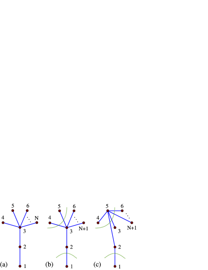
In our first example we consider the $Y_{N}$-state, a generalization of the $Y_{5}$-state, shown in Fig. 2(a). For this family of states we can generalize Theorem 10 and show that the criterion of PPT mixtures is necessary and sufficient. We need the following lemma:

Figure 2: (a) The graph of a $Y_{N}$-state, a possible generalization of the $Y_{5}$-state. (b) A possible 2BP partition, here we have chosen $i=5$ and $j=4$. (c) After local complementation on the qubits $3$ and $i=5$, the qubit $5$ is the “central” qubit. The qubits $4$ and $5$ are then in the condition required to fulfill Lemma 9. See text for further discussion.

Lemma 11. Let $\varrho$ be a $Y_{N}$-graph-diagonal state with $N\geq~{}5$ and consider a 2BP partition. Then, if $\varrho$ is PPT with respect to that partition, it can be written as a PPT mixture using 1BP partitions only.

Proof. We prove the statement by induction. The base case for the induction, $N=5$, has already been proven. For the inductive step, consider the $Y_{N+1}$ graph and a 2BP partition [see Fig. 2(b)]. We denote the two parts of the bipartition as $M$ and $\overline{M}$. One can directly see that qubits $1$ and $2$ must belong to different parts of the partition, otherwise the partition is only 1BP. We assume that $1\in M$ and $2\in\overline{M}.$ Furthermore, of the remaining qubits $\{3,...,N+1\}$ there must be at least one belonging to $M$ and at least one belonging to $\overline{M}.$ Otherwise, the partition would be a one vs. $N$ partition, which can never be a 2BP partition. Since $N\geq 5$ there must be either two qubits from the set $\{3,...,N+1\}$ in $M$ or two qubits from the set $\{3,...,N+1\}$ in $\overline{M}.$ Let us assume that the two qubits $i,j\in\{3,...,N+1\}$ belong to $M$.

Now we apply local complementation on qubit $3$ and then on qubit $i$ [see Fig. 2(c)]. If $i=3$ this changes nothing. Otherwise, the graph is transformed so that qubits $3$ and $i$ are interchanged, hence the qubit $i$ is afterwards the “central” qubit. Qubit $j$ is now only connected to the qubit $i$, and both qubits belong to the same part of the partition.

This, however, is exactly the situation as described in Lemma 9. As in the proof of Lemma 9 we can decouple the qubits $i$ and $j$, and the remaining two states $\varrho^{\pm}$ are $Y_{N}$-graph-diagonal states of $N$ qubits, which are PPT with respect to the given 2BP partition. By the induction hypothesis, these states are PPT mixtures with respect to 1BP partitions. Translating this backwards by inserting again the previously deleted connection finally proves the claim. ∎

Having proven Lemma 11 we can formulate:

Theorem 12. A $Y_{N}$-graph-diagonal state is biseparable, if and only if it is a PPT mixture.

Proof. The proof is essentially the same as that of Theorem 10. We only have to consider 1BP partitions according to Lemma 11 and for them PPT is necessary and sufficient. Note that for the $Y_{N}$ graph there are only 1BP and 2BP partitions, 3BP partitions are not possible. ∎

As with the case of the $Y_{5}$ state discussed after Theorem 10, one can simplify the search for PPT mixtures in the $Y_{N}$ state by concentrating only on the 1BP partitions. This makes it possible to determine separability for $Y_{N}$-graph-diagonal states for larger values of $N$ though the number of 1BP partitions still grows fast.

VII.2 Biseparable decompositions for linear cluster states

For our second example of separability conditions for graph states of more than five particles, let us discuss the six-qubit linear cluster state mixed with white noise. Our goal is to show that the criteria used in this paper allow estimates of separable regions in a simple way even for graph-diagonal states with many qubits, and the resulting estimate is quite accurate.

First, in a straightforward generalization of Lemma 2, many pairs of the form $\sigma=|\!+\!+\!+\!+\!++\rangle\langle\cdot|+|ijklmn\rangle\langle\cdot|$ are separable, the exceptions are the 44 states $\chi_{i}=|\!+\!+\!+\!+\!++\rangle\langle\cdot|+\eta_{i},$ with $\eta_{1}=|\!-\!jk\!-\!++\rangle\langle\cdot|$, $\eta_{2}=|\!-\!jkl\!-+\rangle\langle\cdot|$, $\eta_{3}=|\!-\!jklm-\rangle\langle\cdot|$, $\eta_{4}=|\!+\!+\!-jk-\rangle\langle\cdot|$, $\eta_{5}=|\!+\!-jkl-\rangle\langle\cdot|$, or $\eta_{6}=|\!+\!-jk\!-+\rangle\langle\cdot|$. Furthermore, using the fact that the state from Eq. (20) is separable, one can directly find a biseparable decomposition of

$$\varrho(p)=p|C_{6}\rangle\langle C_{6}|+(1-p)\frac{\openone}{64}$$ (32)

for $p=11/43\approx 0.256.$ Since the state $\varrho(p)$ is known to be entangled for $p>51/179\approx 0.285$ bastian2 the real threshold cannot be much higher and this simple estimate already delivers a good approximation.

This method of constructing biseparable decompositions in the graph basis of linear cluster states can be generalized to an arbitrary number of qubits.

VIII Conclusion

In conclusion, we have considered the problem of detecting genuine multiparticle entanglement in graph-diagonal states for four and five qubits and we have provided complete solutions for many important cases. In addition, we showed how these results allow us to gain insight into this problem for larger numbers of qubits. Since our results deliver optimal criteria, they can be used to test the strength of other entanglement criteria.

We believe that the study of entanglement in graph-diagonal states is an interesting and fruitful area of research. These states are extremely important from the point of view of experiments in quantum information science and, from the theoretical point of view, these states have an elegant description in the stabilizer formalism. Future work would involve formulating detection criteria for other entanglement-related problems for this class of states. For instance, are there necessary and sufficient criteria for other forms of entanglement? This may include the notion of full separability (for first results see Ref. graphdiagonal2 ) or the task of entanglement distillation. Can some multiparticle entanglement measures be computed for these types of mixed states? Both of these questions, and many others like them, are in need of further research.

We thank M. Ali, M. Hofmann, M. Kleinmann and S. Niekamp for discussions. This work has been supported by the Austrian Science Fund (FWF): Y376-N16 (START prize), the EU (Marie Curie CIG 293993/ENFOQI), and the MITRE Innovation Program, Grant 07MSR205.

References

- (1) T. Monz et al., Phys. Rev. Lett. 106, 130506 (2011); D. Leibfried et al., Science 304, 1476 (2004).
- (2) C.-Y. Lu et al., Nature Phys. 3, 91 (2007); X.-C. Yao et al., arXiv:1105.6318.
- (3) P. Neumann, et al., Science 320, 1326 (2008).
- (4) R. Horodecki et al., Rev. Mod. Phys. 81, 865 (2009).
- (5) O. Gühne and G. Tóth, Phys. Reports 474, 1 (2009).
- (6) O. Gühne and M. Seevinck, New J. Phys. 12, 053002 (2010).
- (7) C.-M. Li et al., Phys. Rev. Lett. 105, 210504 (2010); J.-D. Bancal et al., Phys. Rev. Lett. 106, 250404 (2011); M. Huber et al., Phys. Rev. A 83, 040301(R) (2011); J.I. de Vicente and M. Huber, arXiv:1106.5756.
- (8) B. Jungnitsch, T. Moroder, and O. Gühne, Phys. Rev. Lett. 106, 190502 (2011).
- (9) M. Hein et al., in Quantum Computers, Algorithms and Chaos, edited by G. Casati, D.L. Shepelyansky, P. Zoller, and G. Benenti (IOS Press, Amsterdam, 2006), quant-ph/0602096.
- (10) M. Hein, W. Dür, and H.-J. Briegel, Phys. Rev. A 71, 032350 (2005); D. Cavalcanti et al., Phys. Rev. Lett. 103, 030502 (2009); Y.S. Weinstein, Phys. Rev. A 80, 022310 (2009).
- (11) A. Kay, J. Phys. A: Math. Theor. 43, 495301 (2010); A. Kay, Phys. Rev. A 83, 020303(R) (2011); O. Gühne, Phys. Lett. A 375, 406 (2011).
- (12) M. Horodecki and R. Horodecki, Phys. Rev. A 54, 1838 (1996).
- (13) B. Jungnitsch, T. Moroder, and O. Gühne, Phys. Rev. A 84, 032310 (2011).
- (14) J.A. Smolin, Phys. Rev. A 63, 032306 (2001).
- (15) P. Horodecki et al., Phys. Rev. A 62, 032310 (2000).
- (16) See the MatLab package PPTmixer, available at mathworks.com/matlabcentral/fileexchange/30968.
- (17) M. Piani, Phys. Rev. A 73, 012345 (2006).
- (18) F. Benatti, R. Floreanini, and M. Piani, Open Syst. Inf. Dyn. 11, 325 (2004).
- (19) M. Horodecki, P. Horodecki, and R. Horodecki, Phys. Rev. Lett. 80, 5239 (1998).