ON THE THEORY OF STRESS-MAGNETIC FIELD PHASE DIAGRAM OF THE FINITE SIZE MULTIFERROICS: COMPETITION BETWEEN FERRO- AND ANTIFERROMAGNETIC DOMAINS

Abstract

Macroscopic properties of multiferroics, the systems that show simultaneously two types of ordering, could be controlled by the external fields of different nature. We analyze the behavior of multiferroics with antiferro-(AFM) and ferromagnetic (FM) ordering under the action of external magnetic and stress fields. A combination of these two fields makes it possible to achieve macroscopic states with different domain structures. The two-domain state obtained in this way shows a linear dependence of macroscopic strain vs magnetic field which is unusual for AFMs. A small but nonzero stress applied to the sample can also result in the bias of the magnetization vs magnetic field dependence.

1 Introduction

Present-day technologies of information storage are based on the i) combination of the materials with different magnetic, electronic, elastic properties; ii) step-like variation of the magnetic, electronic, elastic properties within a small, nano-sized sample; iii) combined application of different fields to implement the control over macroscopic properties. The first tendency initiated the growing interest in the natural and synthetic multiferroics, i.e., materials that show simultaneously at least two different order parameters (like the magnetic and electric polarization). The second tendency is related to the appearance of a giant variation (as compared with that in homogeneous samples) of macroscopic properties like the magnetoresistance and, as a consequence, the high susceptibility of samples to external fields. The last approach opens a way to produce macroscopic states unreacheable in other ways or the desired states much more effectively. It should be noted that the sensitivity of multiferroics to two fields of different nature instead of one should be much greater than that of the single-ferroics. Really, in multiferroics, two order parameters have different origin and different symmetry and even may appear at different temperatures, while the second-order parameter in single-ferroics, which is also the secondary one, contributes to the values of characteristic fields and susceptibilities, but gives rise to no new qualitative effects. So, we can expect that a combination of two fields in multiferroics results in the variety of states with different symmetries that could be used for the effective information storage.

Many multiferroics show strong magnetoelastic effects along with ferro- or antiferromagnetic (FM and AFM, respectively) and ferroelectric ordering (see, e.g., [1–5]). In this case, the macroscopic properties could be controlled by the simultaneous application of stress and magnetic/electric fields. An external stress can be used for the compensation of internal strains that produce the undesirable backswitching of a ferroelectric polarization in some multiferroics (like BiFeO₃) [4]. Additional stresses could be also produced in the course of epitaxial growth (on a substrate with properly chosen misfit), like it was done, e.g., in Ref. [6]. Such a ‘‘plugged’’ stress can stabilize a certain type of domain structure (e.g., by eliminating undesirable domains) and thus facilitate the control over macroscopic properties by external magnetic/electric fields.

A combination of stress and magnetic/electric fields is also interesting from the fundamental point of view, because these fields have not only different symmetries, but also different tensor nature. Here, we study the behavior of a multidomain magnetic system in the presence of stress and magnetic fields. A good example of such a system can be found among materials that show simultaneously the FM and AFM orderings in various systems of magnetic ions (see, e.g., Mn-based antiperovskites [7, 8] and a high-temperature superconductor Sr₂Cu₃O₄Cl₂ [9]) or in the different parts of a sample (like manganite Pr_0.5Ca_0.5MnO₃ [2, 3], in which the FM and AFM phases coexist in a wide range of the temperature and the field). It is also important that an AFM subsystem is usually a source of the pronounced magnetostrictive strain and thus interacts with a stress, while the FM subsystem is strongly coupled with an external magnetic field. Moreover, in the finite-size samples, the AFM-induced magnetostriction and the FM magnetization are the sources of different shape-induced (destressing and demagnetizing) effects that compete with external fields and may also compete with each other.

The main question which we address below is whether a combination of magnetic and stress fields may reveal some new features and facilitate the control over macroscopic properties of a sample. We will analyze the phase diagrams of the homogeneous and multidomain states and the field dependence of the macroscopic strain and the magnetization. We argue that the presence of the FM component gives rise to a substantial increase in the strain susceptibility to the external magnetic field, and the application of a stress can induce the magnetic bias seen as a shift of the magnetization curve.

2 Combined Influence of a Magnetic Field and a Stress on the Magnetic System: Qualitative Considerations

Let us consider a system that shows simultaneously FM and AFM orderings, no matter how it is realized – as a mixture of phases (like in perovskite manganites [2, 3]) or as a FM+AFM multiferroic (like Sr₂Cu₃O₄Cl₂ discussed in details below). Suppose further that the system shows a noticeable magnetoelastic effect which originates from the coupling between the AFM order parameter and the lattice. Which mechanisms are responsible for the equilibrium domain structure (DS) in this case, and how this DS could be controlled? It is well known that the fraction of FM domains (in a pure FM [10] or in a mixture with the AFM phase [11, 12]) is governed by magnetostatic effects usually described with the stray energy

$$\Phi_{\rm stray}=\frac{V}{2}N_{jk}^{\rm dm}\langle M^{\rm{macro}}_{j}M^{\rm{macro}}_{k}\rangle,$$ (1)

where $\mathbf{M}^{\rm{macro}}$ is the macroscopic magnetization, brackets $\langle\dots\rangle$ mean the averaging over the sample volume $V,$ and the second-rank demagnetization tensor $N_{jk}^{\rm dm}$ depends upon the sample shape.

On the contrary, the AFM vectors themselves do not produce any magnetostatic field. However, due to magnetostriction, an AFM component produces the so-called destressing fields of elastic nature [13] that give rise to the formation of an equilibrium DS.

In the case of an FM+AFM phase mixture, the inclusions of a new (FM or AFM, depending upon the direction of a phase transition) phase could be considered as elastic dipoles (due to the strain misfit between the FM and AFM phases). In the case of AFM+FM multiferroic, the analogous dipoles arise at the sample surface (see [14] for details). In both cases, the elastic dipoles produce long-range fields that could be taken into account phenomenologically with the use of the destressing energy

$$\Phi_{\rm dest}=\frac{V}{2}N_{jklm}^{\rm des}\langle L_{j}L_{k}\rangle\langle L_{l}L_{m}\rangle,$$ (2)

where $\mathbf{L}$ is an AFM order parameter, and the 4-th rank destressing tensor $N_{jklm}^{\rm des}$, like $N_{jk}^{\rm dm}$, depends upon the shape of the sample or/and inclusions and upon the magnetoelastic coupling strength.

Both the stray (Eq. (1)) and destressing (Eq. (2)) contributions to the free energy of a sample constrain a variation of the domain fraction in the presence of external fields. Though both contributions originate from different physical mechanisms and even have different symmetry tensor characters, their values could be comparable in general case and should be taken into account on the same footing.

The influences of a magnetic field and a stress on the DS of the FM+AFM system are also different. The external magnetic field $\mathbf{H}$ discerns the domains with opposite orientations of the macroscopic magnetization $\mathbf{M_{\rm F}}$ of FM (or FM component) and also the domains with the perpendicular orientation of the AFM vector $\mathbf{L}$, as follows from the standard expression for the Zeeman energy (per unit volume):

$$w_{\rm Zee}=-\langle\mathbf{M}^{\rm{macro}}\rangle\mathbf{H}-\frac{\chi}{2}\langle[\mathbf{L}\times\mathbf{H}]^{2}\rangle,$$ (3)

where $\chi$ is the magnetic susceptibility of the AFM subsystem, and the macroscopic magnetization $\mathbf{M}^{\rm{macro}}$ includes a contribution from both FM and AFM subsystems, see below, Eq. (6). It should be stressed that the domains with $\mathbf{L}\|\mathbf{H}$ are always unfavorable in a magnetic field and move away under the field action.

On the contrary, the mechanical stress (described by the symmetric tensor $\sigma_{jk}$) has no effect on the FM component (unless it produces the magnetostriction) but may discern the AFM domains with the perpendicular orientation of $\mathbf{L},$ as can be deduced from the expression for the magnetoelastic energy (where the elastic isotropy is supposed):

$$w_{\rm elas}=-\frac{\lambda}{2c_{44}}\langle L_{j}L_{k}-\frac{\mathbf{L}^{2}}{3}\delta_{jk}\rangle\left(\sigma_{jk}-\frac{{\rm Tr}\phantom{!}\hat{\sigma}}{3}\delta_{jk}\right),$$ (4)

where $\lambda$ is the magnetoelastic constant, $c_{jk}$ are the elastic moduli, and we have omitted the terms related to the isotropic (hydrostatic) pressure as immaterial for the further consideration.

If, for example, a tensile/compressive stress is applied along the $\mathbf{n}\|\mathbf{H}$ axis, then the combined action of the magnetic field and the stress is described by the term (obtained from (3) and (4)):

$$w_{\rm{field}}=-\langle\mathbf{M}^{\rm{macro}}\rangle\mathbf{H}-\frac{1}{2}\left(\chi H^{2}+\frac{\lambda\sigma}{c_{44}}\right)\langle[\mathbf{L}\times\mathbf{n}]^{2}\rangle,$$ (5)

where we introduced the value of stress $\sigma\equiv{\rm Tr}\phantom{!}\hat{\sigma}/3-\mathbf{n}\hat{\sigma}\mathbf{n}$.

It is quite obvious from Eq. (5) that the action of a magnetic field on the AFM subsystem is equivalent to the action of a stress with fixed sign. So, a combination of $\mathbf{H}$ and $\hat{\sigma}$ gives possibility to enhance (if $\lambda\sigma>0$) or wipe out (if $\lambda\sigma\propto-c_{44}\chi H^{2}$) the inequivalence of different AFM domains. Thus, it follows from general considerations that the combined application of a stress and a magnetic field opens a way to act selectively on that or those types of domains and to control macroscopic properties of the sample (such as the magnetization, elongation, magnetoresistance, etc.).

In the next sections, we consider the typical effects produced by two fields in a relatively simple but nontrivial AFM+FM multiferroic Sr₂Cu₃O₄Cl₂.

3 Model

The crystal structure of high-temperature superconducting cuprates Sr₂Cu₃O₄Cl₂ and Ba₂Cu₃O₄Cl₂ consists of Cu₃O₄ planes separated by spacer layers of SrCl or BaCl [15, 17]. Two types of magnetic ions, CuI and CuII (see Fig. 1) form two interpenetrating square lattices within Cu₃O₄ planes.

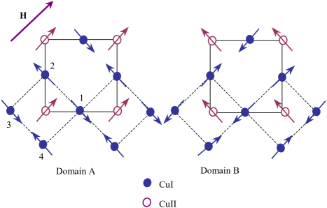
Fig. 1.: (Color online) Magnetic structure of Cu₃O₄ layer in two different configurations (domains). Magnetic field is parallel to $\langle 110\rangle$. Two types of magnetic ions are represented with filled and hollow circles. FM ordered moments of CuII could be (a) parallel (domain A) or (b) perpendicular (domain B) to the applied magnetic field. Small canting of the CuI spins induced by the external magnetic field is ignored

Within the temperature interval $T_{\rm II}\approx 40$ K$\leq T\leq T_{\rm I}\approx 380$ K, the ions of the first type (CuI) are AFM ordered, while the ions of the second type (CuII) bear a small but nonzero FM moment. According to the experiments [18], the mutual orientation of CuI and CuII moments depends upon the direction of the external magnetic field and can be either perpendicular or parallel. In other words, the magnetic structure consists of two weakly coupled subsystems, namely, the AFM subsystem localized on CuI ions and the FM one localized on CuII ions. The FM subsystem is unambiguously described by the magnetization vector $\mathbf{M}_{\rm F}$, and the AFM subsystem is described by two vectors: AFM vector $\mathbf{L}=(\mathbf{S}_{1}-\mathbf{S}_{2}+\mathbf{S}_{3}-\mathbf{S}_{4})/4$ and ferromagnetic vector $\mathbf{M}=\sum_{j}\mathbf{S}_{j}/4$ (numeration of CuI sites is shown in Fig. 1). The macroscopic magnetization $\mathbf{M}^{\rm{macro}}$ (per unit volume) is defined as a sum of FM and AFM magnetizations as follows:

$$\mathbf{M}^{\rm{macro}}=\mathbf{M}_{\rm F}+\mathbf{M}.$$ (6)

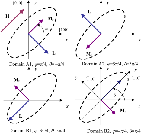
Fig. 2.: (Color online) Four types of magnetic domains. Axes $x$ and $y$ are parallel to $\langle 100\rangle$ crystal directions. The external magnetic field $\mathbf{H}\|[110]$ (if any). Types A and B have different orientations of the AFM vector, types 1 and 2 correspond to opposite directions of the FM vector $\mathbf{M}_{\rm F}$. Ellipse (dash line) images the supposed shape of the sample and its orientation (axes $X$, $Y$) with respect to crystal axes

In the absence of an external field, the FM moments at CuII sites are oriented along $\langle 110\rangle$ crystal directions perpendicular to the staggered magnetizations of the AFM subsystem, as shown in Fig. 1. Due to the tetragonal symmetry of the crystal (space group $I4/mmm$), an equilibrium magnetic structure can be realized in four types of equivalent domains, as shown in Figs. 1 and 2. Domains of type A and B could be thought of as AFM domains, because they correspond to different orientations of the $\mathbf{L}$ vector and thus are sensitive to the orientation of the magnetic field $\mathbf{H}$ or the stress $\hat{\sigma}$ with respect to the crystal axes (see Fig. 2). Types A1 and A2 (and, respectively, B1 and B2) are FM domains; they have opposite directions of the $\mathbf{M}_{\rm F}$ vector and could be removed from the sample by $\mathbf{H}\|\mathbf{M}_{\rm F}$.

If the external (magnetic and stress) fields are applied within the $xy$ (and, equivalently, $XY$) plane and their values are small enough as compared with the exchange interactions between different Cu sites, the magnetic structure of Sr₂Cu₃O₄Cl₂ can be unambiguously described with two angle variables, as shown in Fig. 2:

$$L_{x}=M_{0}\cos\theta,\quad L_{y}=M_{0}\sin\theta;$$

$$M_{{\rm F}x}=m_{\rm F}M_{0}\cos\varphi,\quad M_{{\rm F}y}=m_{\rm F}M_{0}\sin\varphi.$$ (7)

Here, $m_{\rm F}$(=$10^{-3}$ for Sr₂Cu₃O₄Cl₂ [18]) is a dimensionless constant that represents the ratio between the spin moments localized on CuII and CuI sites. We have also taken into account that, far below the Néel temperature, the values of sublattice magnetizations $M_{0}=27.4$ Gs (that corresponds to the spin $s=1/2$ per CuI site) and $M_{\rm F}$ are saturated and constant.

The phenomenological description of the DS is based on the analysis of the free energy potential $\Phi$ of the sample. We consider four constituents of $\Phi$: magnetic $\Phi_{\rm{mag}}$, with account of magnetoelastic interactions; shape-dependent stray (demagnetizing) Eq. (1) and destressing Eq. (2) energies, and the energy $\Phi_{\rm{field}}\equiv Vw_{\rm{field}}$ (see Eq. (5)) of the external fields, as explained above:

$$\Phi=\Phi_{\rm{mag}}+\Phi_{\rm{stray}}+\Phi_{\rm{dest}}+\Phi_{\rm{field}}.$$ (8)

The magnetic energy of Sr₂Cu₃O₄Cl₂ crystal in the mean field approximation is well established [9, 16, 18] and was analyzed in details, along with $\Phi_{\rm{stray}}$ and $\Phi_{\rm{dest}}$, in [19]. Here, we start directly from the simplified expression for the specific potential $\phi\equiv\Phi/V$ expressed through the angles $\theta$ and $\varphi$:

$$\phi=4J_{\rm{pd}}m_{\rm F}\langle\cos(\theta+\varphi)\rangle+K_{\|}\langle\cos 4\theta\rangle-$$

$$-\frac{J^{2}_{\rm{av}}}{8J_{0}}m^{2}_{\rm F}\langle\cos 2(\theta-\varphi)\rangle+\left(\!\frac{H^{2}}{32J_{0}}+\frac{\lambda M_{0}\sigma}{c_{44}}\!\right)\langle\cos 2(\theta-\psi)\rangle-$$

$$-m_{\rm F}H\left[\left(1-\frac{J_{\rm{av}}}{8J_{0}}\right)\langle\cos(\varphi-\psi)\rangle+\right.$$

$$\left.+\frac{J_{\rm{av}}}{8J_{0}}\langle\cos(2\theta-\psi-\varphi)\rangle\right]-$$

$$-N^{\rm des}_{\rm 2an}\langle\cos 2(\theta-\psi)\rangle+\frac{1}{2}M_{0}m_{\rm F}^{2}\left[N^{\rm{dm}}_{a}\langle\cos(\varphi-\psi)\rangle^{2}+\right.$$

$$\left.+N^{\rm{dm}}_{b}\langle\sin(\varphi-\psi)\rangle^{2}\right]+N^{\rm des}\langle\cos 2(\theta-\psi)\rangle^{2}+$$

$$+\Delta N^{\rm des}\langle\sin 2(\theta-\psi)\rangle^{2}.$$ (9)

In (9), $\psi$ is an angle between the unit vector $\mathbf{n}\|\mathbf{H}$ and the $x$-axis, a mechanical stress is applied along $\mathbf{n}$ as described above, $N^{\rm{dm}}_{a,b}$ are the components of the demagnetization, and $N^{\rm des}$, $\Delta N^{\rm des}$ are those of the destressing tensor which are important for the chosen geometry of the sample (thin pillar of the thickness $c$ with an elliptic cross-section, whose principal axes $X$ and $Y$ are parallel to $\langle 110\rangle$ directions within the Cu₃O₄ layers, see Fig. 2), and $N^{\rm des}_{\rm 2an}$ is a shape-induced anisotropy of the AFM subsystem. The meaning and values (in Oe) of phenomenological constants used in (9) are given in Table 1. Here and for the rest of the paper, we use the values in Oe instead of energy units (say, $\phi\rightarrow\phi/M_{0}$, etc.). For the rest of the paper, we assume that the magnetic field and the stress are applied in parallel to one of the principal axes of the sample that coincides with an easy axis for the AFM vector, namely, $\mathbf{n}\|X$, (see Fig. 2), so $\psi=\pi/4$. This situation corresponds to the experimental setup in Refs. [9, 16].

T a b l e  1. : Parameters used in the free energy potential [Eq. (9)]. Raw data in meV taken from [9, 17, 18] are converted to Oe

Parameter	Meaning	Value (Oe)
$J_{0}$	CuI–CuI superexchange (in-plane)	$1.02\times 10^{7}$
$J_{\rm av}$	isotropic pseudodipolar interaction	$-9.4\times 10^{5}$
$J_{\rm pd}$	anisotropic pseudodipolar interaction	$-2.1\times 10^{3}$
$K_{\|}$	in-plane anisotropy $\times 10^{-6}$	$7.8\times 10^{-2}$

4 Homogeneous States in the Presence of Two Fields

Let us start from the analysis of possible homogeneous states that could be realized in the thermodynamic limit (infinite sample, all $N^{\rm{dm}},N^{\rm des}=0$). In this case, the minimization of $\phi$ with respect to the magnetic variables $\theta$ and $\varphi$ gives rise to four solutions labeled as A1,2 and B1,2 (see Fig. 2). Corresponding equilibrium values at $H=0$ and $\sigma=0$ are

$${\textrm{A1:}}\quad\theta_{\rm A1}=-\pi/4,\quad\varphi_{\rm A1}=\phantom{3}\pi/4;$$

$${\textrm{B1:}}\quad\theta_{\rm B1}=\phantom{3}5\pi/4,\quad\varphi_{\rm B1}=3\pi/4;$$

$${\textrm{A2:}}\quad\theta_{\rm A2}=3\pi/4,\quad\varphi_{\rm A2}=5\pi/4;$$

$${\textrm{B2:}}\quad\theta_{\rm B2}=\pi/4,\quad\varphi_{\rm B2}=-\pi/4.$$ (10)

It should be stressed that, in contrast to pure AFMs, the configurations with $(\mathbf{M}_{\rm F},\mathbf{L})$ and $(\mathbf{M}_{\rm F},-\mathbf{L})$ are nonequivalent, due to anisotropic pseudodipolar interactions (described by the constant $J_{\rm pd}$).

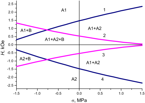
Fig. 3.: (Color online) Stability ranges of different homogeneous states in the presence of a field $H$ and a stress $\sigma$. Solid lines bound the stability ranges of A2 (line 1), B (lines 2, 3) and A1 (line 4) states

In the absence of a field, states A1,2 and B1,2 have the same energy and are equivalent. Stress and magnetic fields remove the degeneracy of these states, as can be seen from the phase diagram shown in Fig. 3. Solid lines in Fig. 3 represent the stability ranges of different states calculated by the direct minimization of potential (9). To calculate the stress values, we used an estimation [19] for the spontaneous strain $u_{0}=\lambda M_{0}^{2}/c_{44}\approx 10^{-6}$.

Lines 2 and 3 correspond to the step-like (spin-flop) transition B1,2$\rightarrow$ A1 (line 2) and A2 (line 3) accompanied by the 90^∘ rotation of the magnetic vectors $\mathbf{L}$ and $\mathbf{M}_{\rm F}$. Within the regions that lie below line 1 and above line 2 (and below line 3 and above line 4), potential (9) has only two minima that correspond to states A1 and A2 with opposite orientations of the magnetic vectors. Such a ‘‘FM’’ state can be induced solely by a magnetic field. The effect of a stress reveals itself in the appearance of the two- or three-state regions (above line 1 (3) and below line 2 (4)), where equilibrium states A1 and B (and A2 and B) have the perpendicular orientation of the magnetic vectors. It is also worth to note the quite general result mentioned in Sec. 2: the application of a stress can either enlarge or diminish (depending on the sign of $\sigma$) the stability regions of homogeneous states and, in that way, invert the order of phase transitions between different states.

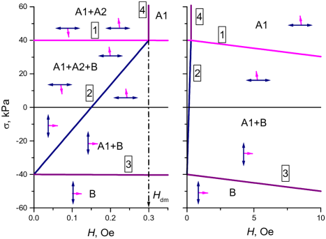
Fig. 4.: (Color online) $\sigma-H$ phase diagram of inhomogeneous states for multiferroic Sr₂Cu₃O₄Cl₂. Left and right panels correspond to different field scales (below and above $H_{\rm dm}$). Solid lines are calculated from the condition of $\xi_{j}=0$, the composition of equilibrium DS is represented schematically in each region. Double-head and single-head arrows show orientations of the AFM and FM vectors, respectively. $\xi^{(0)}=0$ for simplicity

Thus, the combination of a stress and a field opens a way to eliminate any state and, as a result, to produce single-domain states A1 (above lines 1 and 2) or A2 (below lines 3 and 4) and any combination of two- and three-domain states.

In the next sections, we consider the behavior of different multidomain states which appear in the finite-size sample under the application of a stress and a magnetic field.

5 Stability Diagram of a Multidomain State

In a finite-size sample, the equilibrium distribution of the vectors $\mathbf{L}$ and $\mathbf{M}_{\rm F}$ is, in principle, inhomogeneous due to boundary conditions on the sample surface. We consider the multidomain states that consist of homogeneously ordered regions (domains) separated by thin domain walls. No inhomogeneous distribution of $\mathbf{L}$ and $\mathbf{M}_{\rm F}$ within the walls is taken into account. However, we assume that the domain walls can move under ponderomotive, field-induced forces, so that the DS can reach an equilibrium, after the field is applied. The DS is thus unambiguously described by a set of angle variables $\{\theta_{j},\varphi_{j}\}$ ($j$ = A1, A2, B1, B2) and fractions $\xi_{j}$ of domains of the $j$-type. Obviously, $\sum\xi_{j}$=1. The number of free variables in the energy potential (9) depends upon the types of movable domain walls present in the sample. The equilibrium DS in the presence of an external field is then found from the condition for the minimum of $\phi$ with respect to independent variables.

In this section, we consider the case where all four types of domains can freely grow or diminish in size (say, in a virgin sample that initially contains domains of all types). If a stress $\sigma$ and a magnetic field $H$ are rather small (region A1 + A2 + B in Fig. 4), both fields are screened by an appropriate domain configuration, and the effective fields inside the sample are zero. Formally, this means that $\xi_{j}$ are the only free variables. The equilibrium values of the magnetic variables in this case are given by Eq. (10), and the domain fractions depend on the magnetic field and the stress as follows:

$$\xi_{\rm A1,A2}=\frac{1}{4}\left[1-\xi^{(0)}\pm\frac{2H}{H_{\rm dm}}+\left(\frac{H}{H_{\rm des}}\right)^{2}+\frac{\sigma}{\sigma_{0}}\right],$$

$$\xi_{\rm B1}=\xi_{\rm B2}=\frac{1}{4}\left[1+\xi^{(0)}-\left(\frac{H}{H_{\rm{des}}}\right)^{2}-\frac{\sigma}{\sigma_{0}}\right],$$ (11)

where we have introduced the notations

$$H_{\rm{dm}}\equiv m_{\rm F}N^{\rm{dm}}_{a}M_{0},\quad H_{\rm des}\equiv 8\sqrt{J_{0}N^{\rm des}},$$ (12)

$$\sigma_{0}\equiv\frac{2N^{\rm des}c_{44}}{\lambda M_{0}^{2}},\quad\xi^{(0)}\equiv\frac{N^{\rm des}_{\rm 2an}}{N^{\rm des}}.$$ (13)

Physically, $H_{\rm dm}$ is the FM demagnetizing field calculated as if an AFM subsystem is absent. In an analogous way, $H_{\rm des}$ and $\sigma_{0}$ could be treated as the destressing field in the absence of FM ordering expressed in the magnetic and stress equivalents, respectively. The shape-dependent value $\xi^{(0)}$ represents the disbalance between type A and type B domain fractions in the absence of a field. For the sample under consideration (see Table 2), $\xi^{(0)}=0.22$ [19].

T a b l e  2. : Parameters used in numerical simulations. The source of data (experimental or calculated) is specified in the last column. Destressing parameters correspond to $T=120$ K.

Parameter	Meaning	Value	Ref.
$a\times b\times c$	Sample size	$7\times 2\times 0.5$ mm3	[17]
$M_{0}$	Sublatt. magnetization	27.4 Gs	[16]
$m_{\rm F}$	$M_{\rm F}/M_{0}$	$7\times 10^{-4}$	[16]
$M_{\rm F}$	Satur. magnetization	$7\times 10^{-3}$ emu/g	[17]
$\xi^{(0)}$	Shape-induced bias	0.22	[19]
$u_{0}$	Spont. strain	$10^{-6}$	[19]
$H_{\rm dm}$	Demagnetization field	0.3 Oe	Eq.(12)
$N^{\rm des}$	Destressing const.	$7$ mOe	[19]
$H_{\rm des}$	Destressing field	$2.1$ kOe	[19]

As seen from Eq. (12), the value of magnetic destressing field is enhanced due to the exchange interactions (constant $J_{0}$). On the contrary, the demagnetizing field is weakened due to a small FM moment ($m_{\rm F}\ll 1$). So, the demagnetizing field in the crystal under consideration is much smaller than the destressing ones, $H_{\rm dm}\ll H_{\rm des}$ (see Table 2). However, for the chosen geometry of the sample, the demagnetizing and destressing effects are of the same order of value, as will be shown below.

The analysis of Eqs. (11) shows that the type of favorable domain depends upon the sign of $\sigma/\sigma_{0}$. If $\sigma/\sigma_{0}>0$, domains of B type are unfavorable and disappear ($\xi_{\rm B}=0$), when (see line 1 in Fig. 4))

$$\sigma_{\mathrm{B}}=\sigma_{0}\left[1+\xi^{(0)}-\left(\frac{H}{H_{\rm des}}\right)^{2}\right].$$ (14)

A negative stress $\sigma/\sigma_{0}<0$ at $H=0$ can remove domains of A2 type; respectively, $\xi_{\rm A1}=0$ at (line 2 in Fig. 4))

$$\sigma_{\mathrm{A2}}=\sigma_{0}\left[\xi^{(0)}-1+\frac{2H}{H_{\rm{dm}}}-\left(\frac{H}{H_{\rm des}}\right)^{2}\right].$$ (15)

Lines 1 and 2 in Fig. 4 bound the four-domain region and intersect at the point $H=H_{\rm dm}$, $\sigma\approx\sigma_{0}\left(1+\xi^{(0)}\right)$. The two- domain state A1 + A2 consists of FM domains and is stable in the region bounded by lines 1 and 4 (the latter corresponds to $H=H_{\rm dm}$).

Three-domain state A1+B1+B2 (or A1+B, as B1 and B2 are equivalent) is equilibrium in a wide region below lines 2 (Eq. (15)) and 1 (Eq. (14)). The corresponding domain structure can be treated as an AFM one, because there are domains with different orientations of the $\mathbf{L}$ vector that compete with one another. It is worth to note that the negative stress $\sigma/\sigma_{0}<0$ makes the domains of B-type favorable. The magnetization vector $\mathbf{M}_{\rm F}$ of such domains is oriented perpendicularly to an external magnetic field $\mathbf{H}$, as can be seen from the expression for equilibrium fractions

$$\xi_{\mathrm{A1}}=\frac{1}{2}\left[1-\xi^{(0)}+\frac{m_{\rm F}H}{4N^{\rm{des}}}+\left(\frac{H}{H_{\rm des}}\right)^{2}+\frac{\sigma}{\sigma_{0}}\right],$$

$$\xi_{\mathrm{B1}}=\xi_{\rm B2}=\frac{1}{4}\left[1+\xi^{(0)}-\frac{m_{\rm F}H}{4N^{\rm{des}}}-\left(\frac{H}{H_{\rm des}}\right)^{2}-\frac{\sigma}{\sigma_{0}}\right].$$ (16)

In other words, the action of a stress may compensate the action of a field. A negative stress can even remove A1-type domains (with $\mathbf{M}_{\rm F}\|\mathbf{H}$) from the sample. This takes place at the critical line (line 3 in Fig. 4):

$$\sigma_{\mathrm{A1}}=\sigma_{0}\left[\xi^{(0)}-1-\frac{m_{\rm F}H}{4N^{\rm{des}}}-\left(\frac{H}{H_{\rm des}}\right)^{2}\right].$$ (17)

Two more things are also worth noting. First, the lines within the discussed phase diagram of the multidomain state correspond to the reversible (second-order type) transitions realized through the motion of domain walls. In contrast, the irreversible step-like switching between domains (related to the disappearance or nucleation of a certain state) can occur while crossing the stability lines within the phase diagram of the homogeneous state (Fig. 3).

Second, the scale of the reversible phase diagram (Fig. 4) is proportional to a small shape-dependent demagnetizing field $H_{\rm{dm}}=0.3$ Oe and a destressing stress $\sigma_{0}\propto 40$ kPa. The scale of the irreversible phase diagram (Fig. 3) is defined by the intrinsic spin-flop field $H_{\rm{s-f}}\propto 1$ kOe [19] and the characteristic stress scale $\propto 1$ MPa and is at least two orders of magnitude larger. This scale difference is due to the different activation barriers and, hence, different kinetics for the nucleation and the domain wall motion.

In the next section, we consider the behavior of the DS consisting of two types of domains with different orientations of $\mathbf{L}$ vectors.

6 Competition of Two Domains: Nontrivial Field Dependence of Strain

Let us consider a sample which was preliminary monodomainized to state A1 by the excursion into the region of high fields (above lines 1 and 2 in Fig. 3). Suppose that the magnetic field $H$ is then diminished at a fixed stress value, $\sigma$. Which kind of the DS can be expected in this case? It was already shown in [19] that, at $H>0$ and $\sigma=0,$ metastable homogeneous state B has lower energy than homogeneous state A2. The same relation is true for a negative stress, $\lambda\sigma<0$, as the energy of state B in this case is diminished, and also takes place in a rather wide range of positive stress values (between lines 2 and 3 in Fig. 3). So, the nucleation of domains of B type is much more probable than the nucleation of A2-type domains. If, in addition, there is a slight misalignment between the magnetic field $\mathbf{H}$ and a crystal axis [110] that removes the degeneracy between the B1 and B2 states, the DS of the sample is represented by the domains of only two types, A1 and B1.

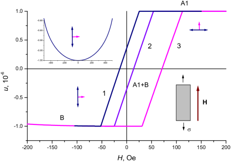
Fig. 5.: (Color online) Field dependence of the macroscopic strain $u(\mathbf{H})$. The sample contains domains of two types, A1 and B. Lines 1, 2 and 3 correspond to $\sigma=0.4$,$-0.4,$ and $-2$ kPa, respectively. Inset shows the same field dependence for a single domain (B-type) sample. Stress and magnetic field are applied as shown schematically in the right bottom angle

To illustrate the peculiarities of macroscopic properties of such two-domain state, we calculated the dependence of the macroscopic magnetization, $\mathbf{M}^{\rm{macro}}$, and the elongation, $u\equiv\langle\mathbf{n}\hat{u}\mathbf{n}-\mathrm{Tr}\hat{u}/2\rangle$ (where $\hat{u}$ is the strain tensor), on the magnetic field $\mathbf{H}$ at a fixed external stress. Equilibrium values of the variables $\{\theta_{j},\varphi_{j},\xi_{j}\}$, $j=A1,B1$, in this case were calculated by the numerical minimization of potential (9), by using the data from Table 2 with limitations $\xi_{\mathrm{A2}}=\xi_{\mathrm{B2}}=0$. The corresponding dependences are given in Figs. 5 and 6.

The particular feature of the dependence $u(\mathbf{H})$ in Fig. 5 is its linearity which is due to the presence of A1 domain with small FM moment. Really, in the single domain A1, the spontaneous strain is constant. In the single domain B $u(\mathbf{H})$ shows the quadratic, symmetric (with respect $\mathbf{H}\rightarrow-\mathbf{H}$) behavior (inset in Fig. 5) that agrees well with the symmetry of the strain tensor with respect to the time inversion (and the corresponding inversion of $\mathbf{H}$). However, in the two-domain case, it is the domain fraction $\xi$ that depends almost linearly on $H,$ thus leading to a nontrivial and unusual field dependence of the strain.

It can be also seen from Fig. 5 that the external stress induces a bias (shift) of the $u(\mathbf{H})$ dependence, which is due to the nonequivalence of domains A1 and B in the presence of a stress. The same bias is induced into magnetization curves (see Fig. 6). The value of bias is controlled by the stress. In thin films, such a bias can be introduced into the sample either by an external stress or by a properly chosen misfit between the film and the substrate.

It is important to emphasize the role of a destressing energy in the field-induced behavior of the strain and the magnetization. In the case under consideration, the demagnetizing (stray) energy is too small to ensure the formation of metastable B-type domains. Really, the demagnetization field $H_{\mathrm{dm}}=0.3$ Oe is much smaller than the characteristic value of magnetic field, at which the appearance of B-type domains is favorable, $H_{\mathrm{cr}}\propto N^{\mathrm{des}}/m_{\rm F}\propto 100$ Oe [19] (see also Figs. 5 and 6). So, the magnetic field-induced switching between A1-type and B1-type domains is possible only due to destressing effects.

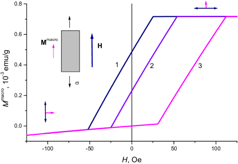
Fig. 6.: (Color online) Field dependence of the macroscopic magnetization $M^{\mathrm{macro}}(\mathbf{H})$. The sample contains domains of two types, A1 and B. Lines 1, 2 and 3 correspond to $\sigma=0.4$, $-0.4,$ and $-2$ kPa, respectively

7 Conclusions

We have considered the behavior of the AFM+FM multiferroic under the action of two external fields of different nature. Our calculations show that such a combination of fields makes it possible to separate the field influence on the different coexisting order parameters. This, in turn, opens a way to control the DS and macroscopic properties and to produce the states with any desirable types of domains.

The simultaneous application of two fields can also increase the susceptibility of a sample to one of the fields, like it is the case with the magnetic susceptibility of a strain. The range of the field values, in which the system is sensible to external fields, can be controlled by the appropriate choice of the sample shape and the corresponding shape-induced ‘‘de-’’ fields (demagnetizing, depolarizing, destressing, etc.).

For the present work, we have chosen the multiferroic with a rather simple, tetragonal structure. However, it would be interesting to generalize the proposed approach to multiferroics with ferroelectric and magnetic order parameters that show simultaneously electro- and magnetostriction (like PZT-PFW systems [20]) or/and have incommensurate AFM structure (like BiFeO₃) that can be realized in more than four types of domains. We believe that three types of possible control fields (electric, magnetic, and stress) in the first case and a large number of possible equilibrium domains in the second case can give rise to some new peculiarities in the macroscopic behavior of multiferroics.

The authors acknowledge the financial support from the Division of Physics and Astronomy of the National Academy of Sciences of Ukraine in the framework of Special Program for Fundamental Research. The work was partially supported by the grant from the Ministry of Education and Science of Ukraine.

ТЕОРЕТИЧНИЙ ОПИС
ФАЗОВОЇ ДIАГРАМИ МУЛЬТИФЕРОЇКIВ
СКIНЧЕННИХ РОЗМIРIВ У ЗМIННИХ МЕХАНIЧНЕ
НАПРУЖЕННЯ–МАГНIТНЕ   ПОЛЕ:    КОНКУРЕНЦIЯ
МIЖ ФЕРО- ТА АНТИФЕРОМАГНIТИМИ ДОМЕНАМИ
О.В. Гомонай, Є. Г. Корнiєнко, В.М. Локтєв
Р е з ю м е
Макроскопiчними властивостями мультифероїкiв, тобто речовин, в яких спiвiснують два типи впорядкування, можна керувати за допомогою полiв рiзної природи. В данiй роботi проаналiзовано поведiнку мультифероїкiв з антиферо- (АФМ) та феромагнiтним (ФМ) впорядкуванням пiд дiєю зовнiшнього магнiтного поля та механiчного напруження. Комбiнацiя цих двох полiв дозволяє отримати макроскопiчнi стани з рiзною доменною структурою. Отриманий таким способом дводоменний стан демонструє нетипову для АФМ лiнiйну залежнiсть макроскопiчної деформацiї вiд зовнiшнього магнiтного поля. Мале, але ненульове механiчне напруження приводить також до зсуву кривої залежностi макроскопiчної намагнiчуваностi вiд магнiтного поля (ефективному ‘‘пiдмагнiчуванню’’).

References

- [1] C.R. dela Cruz, B. Lorenz, Y.Y. Sun, C.W. Chu, S. Park, and S.-W. Cheong, Phys. Rev. B 74, 180402(R) (2006).
- [2] C. Yaicle, C. Martin, Z. Jirak, F. Fauth, G. André, E. Suard, A. Maignan, V. Hardy, R. Retoux, M. Hervieu, S. Hébert, B. Raveau, C. Simon, D. Saurel, A. Brûlet, and F. Bourée, Phys. Rev. B 68, 224412 (2003).
- [3] V. Hardy, S. Majumdar, S.J. Crowe, M.R. Lees, D.M. Paul, L. Hervé, A. Maignan, S. Hébert, C. Martin, C. Yaicle, M. Hervieu, and B. Raveau, Phys. Rev. B 69, 020407 (2004).
- [4] S.H. Baek, H.W. Jang, C.M. Folkman, Y.L. Li, B. Winchester, J.X. Zhang, Q. He, Y.H. Chu, C.T. Nelson, M.S. Rzchowski, X.Q. Pan, R. Ramesh, L.Q. Chen, and C.B. Eom, Nature Materials 9, 309 (2010).
- [5] C. Magen, L. Morellon, P.A. Algarabel, C. Marquina, and M.R. Ibarra, Jour. of Phys. Cond. Matt. 15, 2389 (2003).
- [6] T.H. Kim, S.H. Baek, S.M. Yang, S.Y. Jang, D. Ortiz, T.K. Song, J. Chung, C.B. Eom, T.W. Noh, and J. Yoon, Appl. Phys. Lett. 95, 262902 (2009).
- [7] B.S. Wang, P. Tong. Y.P. Sun, X.B. Zhu, W.H. Song, Z.R. Yang, and J.M. Dai, Jour, of Appl. Phys. 106, 013906 (2009).
- [8] B.S. Wang, P. Tong, Y.P. Sun, X. Luo, X.B. Zhu, G. Li, X.D. Zhu, S.B. Zhang, Z.R. Yang, W.H. Song, and J.M. Dai, Europhys. Lett. 85, 47004 (2009).
- [9] F.C. Chou, A. Aharony, R.J. Birgeneau, O. Entin-Wohlman, M. Greven, A.B. Harris, M.A. Kastner, Y.J. Kim, D.S. Kleinberg, Y.S. Lee, and Q. Zhu, Phys. Rev. Lett. 78, 535 (1997).
- [10] C. Kittel, Rev. Mod. Phys. 21, 541 (1949).
- [11] V.G. Bar’yakhtar, A.N. Bogdanov, and D.A. Yablonskii, Physics-Uspekhi 31, 810 (1988).
- [12] V.G. Bar’yakhtar, A. Borovik, and V. Popov, JETP Letters 9, 391 (1969).
- [13] H.V. Gomonay and V.M. Loktev, Phys. Rev. B 75, 174439 (2007).
- [14] H.V. Gomonay, I. Kornienko, and V.M. Loktev, Condensed Matter Physics 13, 23701 (2010).
- [15] S. Noro, T. Kouchi, H. Harada, T. Yamadaya, M. Tadokoro, and H. Suzuki, Mater. Sci. and Eng.: B 25, 167 (1994).
- [16] Y.J. Kim, R.J. Birgeneau, F.C. Chou, M. Greven, M.A. Kastner, Y.S. Lee, B.O. Wells, A. Aharony, O. Entin-Wohlman, I.Y. Korenblit, A.B. Harris, R.W. Erwin, and G. Shirane, Phys. Rev. B. 64, 024435 (2001).
- [17] B. Parks, M.A. Kastner, Y.J. Kim. A.B. Harris, F.C. Chou, O. Entin-Wohlman, and A. Aharony, Phys. Rev. B 63, 134433 (2001).
- [18] M.A. Kastner, A. Aharony, R.J. Birgeneau, F.C. Chou, O. Entin-Wohlman, M. Greven, A.B. Harris, Y.J. Kim, Y.S. Lee, M.E. Parks, and Q. Zhu, Phys. Rev. B 59, 14702 (1999).
- [19] H.V. Gomonay, I.G. Korniienko, and V.M. Loktev, arXiv:1003.2778 (2010).
-
[20]
A. Kumar, R.S. Katiyar, and J.F. Scott, arXiv:1006.3357
(2010).
Received 21.12.10