False discovery rates in somatic mutation studies of cancer
Abstract
The purpose of cancer genome sequencing studies is to determine the nature and types of alterations present in a typical cancer and to discover genes mutated at high frequencies. In this article we discuss statistical methods for the analysis of somatic mutation frequency data generated in these studies. We place special emphasis on a two-stage study design introduced by Sjöblom et al. [Science 314 (2006) 268–274]. In this context, we describe and compare statistical methods for constructing scores that can be used to prioritize candidate genes for further investigation and to assess the statistical significance of the candidates thus identified. Controversy has surrounded the reliability of the false discovery rates estimates provided by the approximations used in early cancer genome studies. To address these, we develop a semiparametric Bayesian model that provides an accurate fit to the data. We use this model to generate a large collection of realistic scenarios, and evaluate alternative approaches on this collection. Our assessment is impartial in that the model used for generating data is not used by any of the approaches compared. And is objective, in that the scenarios are generated by a model that fits data. Our results quantify the conservative control of the false discovery rate with the Benjamini and Hockberg method compared to the empirical Bayes approach and the multiple testing method proposed in Storey [J. R. Stat. Soc. Ser. B Stat. Methodol. 64 (2002) 479–498]. Simulation results also show a negligible departure from the target false discovery rate for the methodology used in Sjöblom et al. [Science 314 (2006) 268–274].
doi:
10.1214/10-AOAS438keywords:
.and TT1Supported in part by NSF Grant DMS-03-42111.
1 Introduction
The systematic investigation of the genomes of human cancers has recently become possible with improvements in sequencing and bioinformatic technologies. Sjöblom et al. (2006) and Wood et al. (2007) determined the sequence of comprehensive collections of coding genes (CCDS and RefSeq) in colorectal and breast cancers, and provided a catalogue of somatic mutations. In this context, a somatic mutation is a tumor-specific mutation not present in the germline of the patient whose tumor contained it. Subsequently, Greenman et al. (2006) investigated somatic mutations in the coding exons of 518 protein kinase genes in a large and diverse set of human cancers. More recently, mutation data from glioblastoma tissues have been studied in the The Cancer Genome Atlas project (2008) and Parsons et al. (2008), and from pancreatic cancer in Jones et al. (2008). Statistical analysis of the data generated in these studies poses new challenges that are worthy of careful consideration. Greenman et al. (2006) have provided an in-depth analysis of data generated by one-stage studies. To make optimal use of sequencing resources, Sjöblom et al. (2006) introduced a two-stage design, with the stages termed “Discovery” and “Validation.” The Discovery Stage consists of a catalog of mutations in all genes considered, for example, all genes in the CCDS database. This design permitted selection of the subset of genes that harbored at least one somatic mutation, termed “Discovered.” This subset was further investigated in a Validation Stage which cataloged somatic mutations in discovered genes in an independent set of tumor samples. Genes that were mutated in at least one tumor in the Validation set were termed “Validated.” In this article we consider this two-stage design. Sjöblom et al. (2006) and Wood et al. (2007), adopting this experimental design, discovered that among the genes whose mutations are likely responsible for carcinogenesis, the majority, the “hills,” had mutations in small subgroups of cases, while only a handful of genes, the “mountains,” were mutated in large subgroups. Thus, the hills and not the mountains dominate the cancer genome landscape. This imbalance emphasizes the importance of statistical methods in identifying the mutations involved in the carcinogenesis process.
The somatic mutations found in cancer tissues are either “drivers” or “passengers” [Wood et al. (2007)]. Driver mutations are causally involved in the neoplastic process and are positively selected during tumorigenesis. Passenger mutations provide no positive or negative selective advantage to the tumor but are retained by chance during repeated rounds of cell division and clonal expansion. The overarching goal of the statistical analysis of cancer mutation data is to identify genes that are most likely to contain driver mutations on the basis of their mutation type and frequency. This is done by quantifying the evidence that the mutations in a gene reflect underlying mutation rates that are higher than the passenger rates.
Early cancer genome projects provided a rank order of genes by their potential to be drivers of carcinogenesis based on mutation frequencies in tumors as well as the genes’ size and nucleotide compositions. To provide an indication of the significance of lists of possible driver genes, they also provided estimates of the false discovery rate (FDR), that is, the expected proportion of putative drivers that are actually passengers, or the proportion of erroneously rejected null hypotheses [Benjamini and Hochberg (1995)]. Since the seminal article of Benjamini and Hochberg (1995), several authors have proposed alternative methods that control the FDR with improved operating characteristics. Important contributions include relaxing the independence assumption among the test statistics and handling discrete statistics [Benjamini and Yekutieli (2001)]. Reviews are given in Dudoit, Shaffer and Boldrick (2003), Cheng and Pounds (2007) and Farcomeni (2008). Despite a rich literature, applications often include heuristic arguments and, in most cases, the choice of a method is far from trivial: a trade-off arises between methods which have been proved through rigorous analytical arguments to control the FDR under a specified threshold and less conservative procedures that rely on heuristic arguments, examples and asymptotic theory. The trade-off between methodological rigor and operating characteristics becomes particularly relevant, for example, when the independence hypothesis is inappropriate or when data are highly discrete. Applications often ignore these problems.
In this article we consider methods that are specific to somatic mutation analysis, and assess them by a novel model-based approach. Our idea is to develop a “super partes” model that can be used to provide highly realistic artificial datasets for method evaluation. We refer to these as data-driven simulated scenarios. Our scheme for evaluating alternative methods can take into account possible discrepancies between methods’ assumptions and the data. We apply this comparison method by revisiting the Sjöblom et al. (2006) methodology as well as the alternative approaches proposed shortly afterward by several groups [Forrest and Cavet (2007), Getz et al. (2007), Rubin and Green (2007) and Parmigiani et al. (2007a, 2007b)]. We discuss the application of this scheme to the data collected in Wood et al. (2007).
The article is structured in 5 sections. In Section 2 we introduce the notation for modeling mutation counts in tumor tissues and present our probability model. In Section 3 we briefly review techniques for controlling or estimating false discovery rates, and specific approaches for the analysis of somatic mutation data. In Section 4 we compare these approaches. Final remarks are given in Section 5.
2 Data-driven simulation scenarios
2.1 Approach
The idea of data-driven simulations is structured in two steps. First we select a flexible probability model for the observed mutations. The model includes model-specific parameters, genes-specific latent variables and observable mutation counts. The model is consistent with widely established assumptions on carcinogenesis. Prior distributions on the unknown model parameters are specified by using both external experimental results and heuristic data-driven approaches. Second, we infer the genes-specific latent variables, including driver status, through a Monte Carlo Markov chain (MCMC) algorithm and generate simulated data sets consistent with the Wood et al. (2007) study.
Throughout the article this Bayesian model is used only for generating simulated data sets that are highly consistent with the observed data in Wood et al. (2007) and are impartial to the FDR approaches examined. In principle, the model could be used directly for selecting genes having high posterior probabilities of being drivers. Other potential applications of the model include (i) predicting the experimental outcomes for ongoing studies, (ii) optimally choosing the resource allocation for the validation stage using a decision theoretic approach and, more generally, (iii) developing adaptive strategies for sequencing experiments. Nevertheless, here we prefer limiting our comparisons to highly computationally efficient methods whose operating characteristics can be assessed via Monte Carlo techniques over a large number of data sets. Moreover, it would be circular to simultaneously use our Bayesian model for FDR estimation and for generating data for evaluation. As noted in Getz et al. (2007), the performance of some methods could be sensitive to the distribution underlying the experimental data; using a probability model that fits the observed data, but also averages across plausible values of the unknown parameters, allows us to provide appropriately objective comparisons.
| Mutation counts | |
|---|---|
| number of mutations of type detected in gene in the Discovery Stage. | |
| number of mutations of type detected in gene in the Validation Stage. | |
| Coverage | |
| coverage of type in gene in the Discovery Stage. | |
| coverage of type in gene in the Validation Stage. | |
| Mutation rates | |
| rate of mutation of type in the Discovery Stage. | |
| rate of mutation of type in the Validation Stage. | |
| multiplicative gene-specific random effect. | |
2.2 Sampling model
While cancer genome sequencing projects produce a wealth of information, in this article we will focus on the somatic mutation counts, broken down by gene and context, and considered separately for the Discovery and Validation Stages. Table 1 summarizes the notation we will use. Our model applies to a single disease, say, colorectal cancer, at a time. The probability model is defined on the basis of a few well-established assumptions that allow to specify a distribution of mutation counts conditional on unknown gene-specific mutation rates. Using latent variables, we specify a model allowing for unknown composition of the genome in terms of passengers and drivers, and for heterogeneous mutation rates across driver genes. More formally, we assume that, for each gene and sample, the number of mutations of type , that is, the number of identical mutations that can occur only in a specific context, for example, C to G in a CpG locus, is a mixture of Poisson distributions,
| (1) |
where indexes a tumor, indexes a gene and denotes the coverage, or the number of successfully sequenced nucleotides susceptible to mutation of type in gene and sample . The parameter represents the rate of mutations of type among passengers. The multiplicative factor is designed to capture the fact that the abundance of mutations varies across tumors. The transition of a tissue from normal to cancer can be described as a progressive accumulation of mutations, some of them are drivers and some are passengers. This dynamic varies across tumors; such heterogeneity is the focus of a significant portion of cancer research; see Stratton, Campbell and Futreal (2009) for a stimulating discussion. Our model, as well as those used in the previously mentioned cancer studies, describes a snapshot of this dynamic process at the time of sequencing. The product can be interpreted as the rate of mutations of type in tumor , assuming that the nucleotide is part of a passenger gene. The gene-specific latent variables capture gene-specific variation across the genome; if , gene is a passenger, while higher values identify the drivers. Our model assumes that the rates of mutation across different types of mutations in a single gene are proportional to the rates of mutation in a passenger gene. Finally, is the distribution of ’s across the genome. It allows for values of or bigger and allows for a concentration of mass on the value of , corresponding to the passengers.
The overall structure of the model reflects the assumption that the drivers have higher rates of mutation than the passengers. The analyses in Sjöblom et al. (2006) and Wood et al. (2007) were aimed at selecting cancer genes with mutation rates higher than the hypothesized passenger rates. The use of the Poisson distribution in (1) is motivated by the fact that, under mild assumptions, it well approximates a more rigorous multinomial model [Wood et al. (2007)] obtained by modeling possible mutations in a single gene as binary variables.
Values of individual passenger rates can be obtained using data external to the somatic mutations counts [Sjöblom et al. (2006), Wood et al. (2007)]. This allows us to simplify the model (1) by collapsing data across patients. Once the intensities are known, the collapsed counts data are sufficient statistics for evaluating the likelihood function. This allows for a considerable reduction of the computational requirements. We will thus use the alternative representation of (1):
| (2) |
where is the total number of mutations of type harbored in the th gene, and .
Multistage designs are attractive strategies for identifying cancer genes; the first stage indicates a subset of genes that are more likely to be drivers and, in the subsequent phase, only this subset is analyzed. Relevant cost–effectiveness analysis and comparisons of alternative designs for genome-wide studies are illustrated in Satagopan et al. (2002), Satagopan and Elston (2003), Satagopan, Venkatraman and Begg (2004), Kraft (2006), Skol et al. (2006), Wang and Stram (2006) and Parmigiani et al. (2009). In the studies discussed by Sjöblom et al. (2006) and Wood et al. (2007), at the end of the first stage all genes which harbored one or more mutations are considered for further study. We will use the notation and for denoting the number of mutations in the two phases. Similarly, and denote the coverages and the rates for the discovery and validation phases. Model (2) can be adapted to the two-stage design as follows:
| (3) | |||||
In these expressions the coverages and are considered fixed. While some variation may be experimentally observed, this is unlikely to be related to a gene’s driver status, and, thus, it is appropriate to model the data conditionally on the coverages. For our purpose, the following three considerations are critical:
Two-stage design. Only genes that harbor at least one mutation in the Discovery Stage are sequenced in the Validation Stage. This screening condition needs to be taken into account when assessing significance using -values or other methods that rely on the sampling distribution.
Coverage. The number of nucleotides successfully sequenced is generally smaller than the gene length times the number of tumors analyzed. For example, certain exons may be technically challenging to sequence. It is appropriate to apply stringent quality criteria to sequencing data, which lead to the exclusion of nucleotides whose sequence could not be identified with certainty. Nucleotides excluded, or not covered, should not be included in statistical evaluations. In what follows -values and other statistics used for prioritizing putative driver genes are computed taking into account, for each gene, which loci have been sequenced.
Context. The third consideration involves the observed bases in the mutations. In sequencing studies, the precise bases that comprise the mutation, as well as the neighboring bases, termed “mutation contexts,” are important. We use a classification of contexts provided in Wood et al. (2007). This is a partition of the sequenced basis. For our purpose, it is relevant that each subset has specific rates of mutation under the passenger status. This fact implies that the priority given to a gene in further studies and the statistical significance of a gene should depend not only on the number of nucleotides but also on the gene-specific basis sequence.
2.3 A Bayesian approach to generating simulation scenarios
For our analysis we propose embedding the sampling model (2.2) in a Bayesian semiparametric model. This will allow us to generate possible scenarios consistent with the data from the Wood et al. (2007) study. We use a Dirichlet process prior [Ferguson (1973)] for the unknown distribution ,
| (4) |
where is a positive measure on . Reviews on the Dirichlet process and applications in biostatistics are given in Dunson (2010) and Müller and Quintana (2004).
We chose the Dirichlet mixture model because of its flexibility compared to alternative parametric prior distributions. Simple preliminary analysis of the mutation data shows that the so-called mountains can have mutation rates over 100-folds higher than the passengers, while hills have markedly lower rates. To capture both the mountains and the hills, we specify a sufficiently flexible prior on the unknown mixing distribution . As shown in Venturini, Dominici and Parmigiani (2008), Bayesian mixtures model effectively heavy tail distributions; in contrast, the posterior behavior of more parsimonious parametric models can be strongly biased.
In order to generate scenarios consistent with the data in Wood et al. (2007), we use a Monte Carlo Markov chain algorithm discussed in Escobar and West (1995). The sampler is based on the Polya urn representation of the Dirichlet process [Blackwell and MacQueen (1973)] and has been studied for posterior simulation under the generic Dirichlet mixture model
The only condition for implementing the sampling scheme of Escobar and West (1995) is that for every subset of distinct integers ranging from to , the integral
| (5) |
can be easily computed. To this end, we specify the prior parameter proportional to a spiked distribution, including a point mass at and a shifted gamma distribution with support , that is,
| (6) |
where is a Dirac measure, is the indicator function and are strictly positive. It can be verified that this choice of allows us to analytically solve integral (5).
We chose the mean of the random distribution by a simple procedure. We recall that the centering distribution of the Dirichlet process is ; for every subset of the real line, if , then , a priori, is beta distributed, with mean ; see Ferguson (1973). In order to specify the centering distribution, we first compute the maximum likelihood estimator of the mixing distribution in (2.2). Then, we specify the parameter , this is the a priori expectation of the unknown proportion of passenger genes. In what follows is set equal to . Finally, the parameterization of the centering distribution is completed by setting and in (6) so that the means and variances of the two distributions and are identical. The steps outlined have clear interpretations, nevertheless, the choice is, to some extent, arbitrary; we also implemented posterior inference for alternative prior parameterizations: these include equal to , and . We did not observe marked sensitivity; for example, the ratio between the maximum and the minimum posterior estimates of the number of drivers is equal to 1.06.
We use the contexts and mutations classification discussed in Wood et al. (2007). This classification is important because it allows us to account for variations in the rates of mutations for passengers across loci, with rates depending on the basis sequences. This classification includes 25 possible types of mutations (). The rates for the 1st and the 2nd stage were measured using SNP data. The SNP-based approach estimates the passenger mutation rates by comparing the nonsynonymous to synonymous mutation ratios in cancer and normal tissues. This approach has been considered in Wood et al. (2007). It estimates the passenger rates using sequencing data from loci which are known for not contributing to carcinogenesis, and thus are not positively selected during carcinogenesis; this characteristic is the defining feature of passenger genes.
A key advantage of the Bayesian estimate of the mixing distribution, compared to the maximum likelihood estimate , is that it allows us to fully take into account the uncertainty on the distribution of rates across genome, and to produce data sets under many different plausible versions of this distribution.
The MCMC algorithm outlined, after a sufficient number of burn-in iterations, produces approximate samples from the conditional distribution of the latent variables given the data. The number of burn-in iterations can be assessed by means of standard diagnostic procedures for MCMC methods; see, for example, Smith (2007). Each iteration of the MCMC algorithm provides a collection of ’s which is used as a simulation scenario. For each scenario we generate a single data set using (2.2). Each scenario can be used to evaluate a given list of putative drivers by checking the proportion of genes in the list for which .
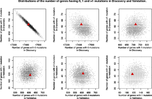
To highlight the excellent fit we obtain, Figure 1 provides an overview of 10,000 scenarios sampled by means of the proposed approach. Each iteration attempts to reproduce the experiment on colorectal tumors discussed in Wood et al. (2007). They considered 18,190 genes. During the discovery phase, all genes were sequenced in 11 tumors. During the validation phase, 769 genes were sequenced in 24 tumors. In the discovery phase, 17,421 genes did not harbor any mutation, 716 genes harbored 1 mutation and 53 genes harbored more than 1 mutation. In the validation phase, 609 did not harbor any mutation, 115 harbored 1 and 45 harbored more than 1. Figure 1 represents the distribution, across the simulated scenarios, of the number of genes harboring 0, 1 or more than 1 mutations in the two stages. As appropriate, scenarios vary in their number of mutated genes found, while distributions are centered around the observed data.
The data-driven simulation approach requires the variability across simulations to be consistent with the data. In principle, if the experiment was repeated several times, one would like to observe a similar degree of variability across simulations and across experiments. In practice, the degree of variability across simulations can be critically evaluated by means of inferential arguments. The bootstrap method is specifically designed for predicting, on the basis of a single experiment, the degree of variability across independent replicates of the experiment. We compared the degree of variability across simulations, illustrated in Figure 1, with the variability estimates obtained by bootstrapping. Our application of the bootstrap builds on parametric estimates, for each gene, of the probabilities , , and , obtained by fitting logistic binary regression models; these estimates are functions of the gene-specific coverages . The degree of uncertainty represented in Figure 1 agrees with the bootstrap estimates; the ratios between the standard deviations of the six univariate empirical distributions illustrated in Figure 1 and the corresponding bootstrap estimates range between 1.03 and 1.17. Note that the six variables considered in Figure 1 define a coarse partition of the genes; more generally, one can use the bootstrap method for assessing the degree of variability of other marginal distributions.
3 Alternative methods for controlling the FDR
In this section we review alternative FDR methods, we will then compare their operating characteristics by means of the simulations described in the previous section.
3.1 The Benjamini and Hochberg, and the Storey procedures
Benjamini and Hochberg (1995) considered which of the null hypotheses , if any, should be rejected given -values , one for each hypothesis. They proposed a procedure for rejecting a (possibly empty) subset of hypotheses so as to control the FDR, that is,
| (7) |
with the proviso that the above ratio is when none of the hypotheses is rejected. The expectation in (7) is with respect to the unknown joint distribution of the test statistics . The input of the procedure is the vector and the output is the subset of rejected hypotheses. The -values corresponding to the true null hypothesis are independently uniformly distributed. The FDR is an attractive error measurement in many applications with massive multiple hypotheses testing; we refer to Dudoit, Shaffer and Boldrick (2003) for a comparison with alternative error measurements.
Let be the sorted values in ascending order of the -values and let be any desired upper bound for the FDR. Benjamini and Hochberg (1995) proved that the procedure that rejects the hypotheses with a -value lower than
| (8) |
controls the FDR below . They show that, for every hypothetical proportion of the true null hypothesis,
| (9) |
The above inequality shows that the procedure is conservative. Storey (2002) studied an alternative step-up method which starts from an estimate of the proportion of the true null hypothesis and then set a threshold similar to (8) indicating the rejection region. The estimate and the inequality (9) are used for inflating the upper bounds , , in (8). The estimate of is based on the right tail of the empirical distribution of the -values.
3.2 The empirical Bayes method
The use of empirical Bayes procedures for estimating the FDR has been discussed by several authors, including Efron et al. (2001), Efron (2003) and Dudoit, Gilbert and Laan (2008). In this approach, one computes a data summary, or score , that captures departure from the null hypothesis, such as a -value, a likelihood ratio or other statistics. In our case, should capture evidence for the rate of mutation for gene being higher than the passenger rate. The empirical Bayes method is based on a mixture representation of the distribution of these scores:
| (10) |
is the distribution of a randomly selected score, is the unknown proportion of true passengers, is the distribution of a score randomly selected among passengers and, finally, is the distribution of scores among drivers. The objectives are estimating the conditional probabilities
and identifying a rejection region containing the more significant scores, such that
| (11) |
where is the target ratio between the mistakenly rejected hypothesis and the total number of rejections.
The distribution can be approximated simulating the scores assuming the genome only consists of passenger genes [Wood et al. (2007)], while the distribution and the proportion are usually estimated by smoothing the scores’ empirical distribution. Finally, expression (11) is used for rejecting a subset of null hypothesis in such a way that the estimated proportion of erroneously rejected null hypothesis is lower than .
There is an important difference between the Benjamini and Hochberg (1995) method and the empirical Bayes method. The former rejects a subset of a list of null hypotheses and controls the expected proportion of erroneously rejected hypotheses. The latter, for a generic rejection region, estimates the proportion of true null hypotheses; the investigator can then select a subset of hypothesis such that the estimate is lower than a desired threshold .
3.3 The CaMP score
Sjöblom et al. (2006) introduced the cancer mutation prevalence (CaMP) score, to provide a ranking of the Validated genes and select promising candidates. The score is based on the probability of observing the number of actually found mutations if the gene was a passenger gene, using a binomial model:
| (12) |
Recall that and are expected proportions of nucleotides, in a passenger gene, harboring mutations of type . The model takes into account the two-stage experimental design.
We then rank the ’s and call the resulting ranks. The CaMP score is defined as
and
The top row corresponds to genes that are eliminated at the Discovery or Validation Stage. The goal of the CaMP score is to rank genes according to the strength of the evidence that they may be mutated at rates higher than the passenger rates. An advantage of CaMP scores is that they can be easily computed. This definition can also be seen as an approximation of the Benjamini and Hochberg (1995) procedure. In Sjöblom et al. (2006) a threshold of 1 on the CaMP scores was considered to generate a list of putative drivers, with the goal of producing a list having approximately 10% of erroneously discovered drivers. The probabilities are not -values because they are not tail probabilities, but can be used as approximation of the -values if the expected number of mutations in each gene is close to .
Forrest and Cavet (2007) proposed to use tail probabilities for controlling the FDR, though they use a sampling model that does not account for the two-stage design. Getz et al. (2007) emphasized that -values can be used for controlling the FDR and proposed alternative test statistics. The closer test statistics to the CaMP score are obtained by computing the distribution of , under the hypothesis that the th gene is a passenger gene, and evaluating the resulting tail probability. This procedure produces -values which can be used for controlling the FDR by applying the Benjamini and Hochberg (1995) method. Getz et al. (2007) noted that the CaMP score is not a monotone transformation of the probabilities ; that is, given two genes and , it can happen that and . Getz et al. (2007) also discussed the idea of controlling the FDR by using the log-likelihood ratio, that is,
where represents the hypothesis that gene is a passenger and is the gene-specific maximum likelihood estimate. Rubin and Green (2007) proposed to use the tail probabilities , based on the aggregate number of mutations in a gene. These critiques of the analysis in Sjöblom et al. (2006) and the alternatives proposed by these authors suggest the idea of systematically assessing the operative characteristics of alternative approaches. Our comparisons in Section 4 consider the CaMP score and the alternative -values proposed by Getz et al. (2007), Forrest and Cavet (2007) and Rubin and Green (2007). These alternative statistics are used for implementing both the Benjamini and Hochberg (1995) method, the method discussed in Storey (2002) and the Empirical Bayes method.
4 Simulation study
In this section we compare alternative methods for identifying driver genes using the 10,000 simulation scenarios described in Section 2. The Wood et al. (2007) study considered both colon and breast tumors. Here we consider each tumor type separately, and repeat the same analysis.
| False discoveries | Average number of | ||||
|---|---|---|---|---|---|
| proportion | selected genes | ||||
| Scores | |||||
| Method | or -values | ||||
| Colon-based simulations | |||||
| BH | CaMP score | 0.101 | 0.218 | 150.4 | 221.8 |
| BH | 0.074 | 0.146 | 115.1 | 198.7 | |
| BH | likelihood ratio | 0.071 | 0.144 | 135.2 | 208.2 |
| EB | CaMP score | 0.106 | 0.232 | 162.3 | 242.6 |
| EB | 0.100 | 0.238 | 147.8 | 250.4 | |
| EB | likelihood ratio | 0.102 | 0.211 | 163.8 | 237.2 |
| ST | CaMP score | 0.104 | 0.220 | 157.3 | 235.4 |
| ST | 0.099 | 0.232 | 146.5 | 242.4 | |
| ST | likelihood ratio | 0.100 | 0.207 | 159.0 | 231.6 |
| Breast-based simulations | |||||
| BH | CaMP score | 0.098 | 0.196 | 146.6 | 218.8 |
| BH | 0.075 | 0.150 | 119.4 | 193.7 | |
| BH | likelihood ratio | 0.074 | 0.141 | 131.7 | 205.3 |
| EB | CaMP score | 0.108 | 0.216 | 158.2 | 226.7 |
| EB | 0.105 | 0.225 | 139.6 | 235.0 | |
| EB | likelihood ratio | 0.098 | 0.209 | 153.5 | 223.4 |
| ST | CaMP score | 0.103 | 0.213 | 157.6 | 219.5 |
| ST | 0.101 | 0.222 | 136.8 | 228.6 | |
| ST | likelihood ratio | 0.096 | 0.207 | 147.6 | 221.2 |
Our simulation study compares the performance of alternative methods for ranking cancer genes and selecting putative cancer genes. Table 2 provides the average operating characteristics across all the simulated scenarios. All methods are set to control the FDR at 10% and 20% levels in turn. The empirical Bayes method estimates the FDR: the investigator controls the FDR by approximately matching the desired level and the estimated proportion of false discoveries. Table 2 shows the average proportion of genes erroneously classified as drivers. Our results emphasize that operating characteristics are quite conservative when the FDR is controlled, on the basis of alternative -values, using the Benjamini and Hochberg (1995) procedure. They also illustrate the importance of quantifying this conservative behavior by contrasting it with alternative methods such as the method proposed in Storey (2002) and the Empirical Bayes method. The Bayesian model of Section 2 allows us to simulate mutations across the genome, while the operating characteristics of the alternative methods shown in Table 2 provide approximations of their performances. The interpretation of the simulation study is anchored to the modeling assumptions formalized in Section 2. The results provide a solid basis for choosing among alternative methods.
All the methods considered produce lists of putative drivers genes with an average misclassification error below the 11% when the control of the FDR is set at the 10% level. If the desired level is 10 %, our results indicate that, when the CaMP scores are adopted, with the Benjamini and Hochberg (1995) procedure, the average proportion of false discoveries is approximately equal to , while under the empirical Bayes method and the Storey (2002) method, a slight excess of false discoveries is observed. We note, both in the colon and breast simulation studies, that the use of the likelihood ratios or the -values with the Benjamini and Hochberg (1995) procedure, on average, selects a substantially lower number of putative drivers than the alternative approaches. When the likelihood ratio and the -value are compared, under the empirical Bayes method and the Storey (2002) method, the likelihood ratio seams preferable; the average proportions of false discoveries are similar, but the likelihood ratio statistics select larger sets of putative drivers than the -values . Also, when comparing the empirical Bayes method and the Storey (2002) method based on the likelihood ratio statistics, we observed only small variations both in the average proportion of false discoveries and in the average number of putative drivers. The operating characteristics when is set at the 20% level confirm the conservative behavior of the Benjamini and Hochberg (1995) procedure with the likelihood ratios or the -values , but also show departures from the target FDR of the Empirical Bayes method and the Storey (2002) method. These results hold for both colorectal and breast cancer. When is equal to 20%, the likelihood ratio seems preferable to the -value , under both the empirical Bayes method and the Storey (2002) method; the likelihood ratios select putatitive drivers with an average misclassification error closer to the 20% target than the -values.
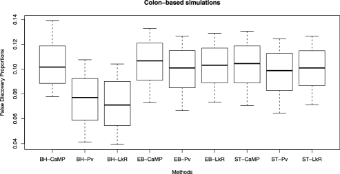
The simulation-based comparison also allows us to asses the variability of the false discoveries proportion across scenarios, summarized in Figure 2. Each box plot is representative of the simulation-based distribution of the proportion of erroneously rejected hypothesis. The degree of variability is similar for all the methods considered; this similarity indicates that the average operating characteristics concisely reported in Table 2 are sufficient for a reliable evaluation of the methods.
To illustrate the importance of accounting for the two stages of the experimental design in computing tail probabilities , we repeated the analysis ignoring the two-stage structure. That is, we computed the tail probabilities under the erroneous assumption that the mutation counts were observed in a single stage experiment. We observed a substantial reduction of the average number of selected genes, across simulation scenarios, when the tail probabilities are used for implementing the Benjamini and Hochberg (1995) procedure; with in the colon cancer and breast cancer cases, the averages become and respectively, and, with , they decrease to and .
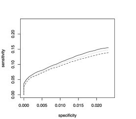
Another important question concerns the fidelity of the ranking provided by these statistics. Figure 3 shows the Bayesian estimates of the left side of the ROC curves corresponding to each of the scores considered. The ROC curves are computed by separately estimating the scores’ distributions across drivers and across passengers. The partial area under the curve is truncated at the 2% specificity level. This is equal to for the log-likelihood ratio test statistic, for the -values and for the CaMP scores. The ROC curves estimates suggest that the log-likelihood ratio test statistic provides best discrimination, though differences are small.
5 Discussion
The investigation of somatic alterations is of primary interest in cancer research. Recent sequencing technologies have brought new insight into this question by revealing a landscape characterized by mutations involving a large number of driver genes, each altered in a relatively small fraction of tumors. When the earlier of these studies began to emerge, the cancer research community was faced with unexpected heterogeneity and complexity, which required a significant change of perspective in both basic and clinical cancer investigations. The earliest genome-wide investigations [Sjöblom et al. (2006)] proposed this change of landscape based on a relative small number of samples. A key element in support of this proposal were estimates of the statistical significance of the reported list of driver genes [Sjöblom et al. (2006)]. These estimates were challenged: alternative approaches were proposed which would have led to reporting a drastically reduced number of candidate drivers at the same significance level.
Subsequent studies have provided strong supporting evidence for this new landscape, as well as validation for the driver role of many of the individual genes initially identified in Sjöblom et al. (2006). However, from a statistical standpoint, it remains very interesting to understand whether the initial conclusion was statistically sound based on the evidence available at the time, in part because similar problems will arise again in other cancer types and in other fields of genomics and evolutionary biology. Thus, our focus in this article has been the rigorous evaluation of methods for the identification of driver genes, with special emphasis on the methods that have been instrumental in the change of landscape we just described.
In the statistical literature, two common approaches for the evaluation of methodologies are asymptotic properties and scenario-based simulation studies. Asymptotic conclusions can be difficult to extrapolate to small samples. Scenario-based simulations can lack objectivity and comprehensiveness, and it can be a challenge to gauge whether the conclusions are applicable or not to a specific context of interest. To overcome these difficulties, we have proposed and implemented an alternative concept, which we hope will be very broadly applicable across statistics, and contribute to a more objective assessment of alternative methods. The idea is to construct a “super partes” model that is (a) independent of the approaches being compared; (b) fits the data and available substantive knowledge well; and (c) can produce artificial data sets accounting for all relevant uncertainties, including parameter and potentially model uncertainty. This model is then used to simulate objective data-driven scenarios for method comparison. In this article our implementation of the super-partes model is based on Bayesian nonparametrics, an approach that can satisfy all three of the requirements above.
Strengths of the approach we proposed are the clear interpretation of both the assumptions captured by the Bayesian model and the average operating characteristics. The probability model’s ability to reproduce the data structure allows to effectively interpret the results. The proposed evaluation scheme could be extended further to allow for more complex assumptions such as dependency among genes belonging to common functional pathways.
When applied to the controversy surrounding FDR control of early cancer genome studies, our method shows that the estimates provided in Sjöblom et al. (2006) are quite accurate despite the approximations used. Also, the Benjamini and Hochberg (1995) method is severely conservative. Last, the Empirical Bayes method and the Storey method based on likelihood ratios emerge as the preferred choices, though the margin of improvement is dependent on the control level.
Acknowledgments
We thank the Editor and two referees for helpful comments. We thank Ken Kinzler, Victor Velculescu and Bert Vogelstein for sharing their invaluable insight on the issues discussed in our analysis.
References
- Benjamini and Hochberg (1995) {barticle}[mr] \bauthor\bsnmBenjamini, \bfnmYoav\binitsY. and \bauthor\bsnmHochberg, \bfnmYosef\binitsY. (\byear1995). \btitleControlling the false discovery rate: A practical and powerful approach to multiple testing. \bjournalJ. Roy. Statist. Soc. Ser. B \bvolume57 \bpages289–300. \bidmr=1325392 \endbibitem
- Benjamini and Yekutieli (2001) {barticle}[mr] \bauthor\bsnmBenjamini, \bfnmYoav\binitsY. and \bauthor\bsnmYekutieli, \bfnmDaniel\binitsD. (\byear2001). \btitleThe control of the false discovery rate in multiple testing under dependency. \bjournalAnn. Statist. \bvolume29 \bpages1165–1188. \biddoi=10.1214/aos/1013699998, mr=1869245 \endbibitem
- Blackwell and MacQueen (1973) {barticle}[mr] \bauthor\bsnmBlackwell, \bfnmDavid\binitsD. and \bauthor\bsnmMacQueen, \bfnmJames B.\binitsJ. B. (\byear1973). \btitleFerguson distributions via Pólya urn schemes. \bjournalAnn. Statist. \bvolume1 \bpages353–355. \bidmr=0362614 \endbibitem
- The Cancer Genome Atlas project (2008) {bmisc}[auto:STB—2010-11-18—09:18:59] \borganizationThe Cancer Genome Atlas project. (\byear2008). \bhowpublishedComprehensive genomic characterization defines human glioblastoma genes and core pathways. Nature 455 1061–1068. \bnote10.1038/nature07385 \endbibitem
- Cheng and Pounds (2007) {bmisc}[auto:STB—2010-11-18—09:18:59] \bauthor\bsnmCheng, \bfnmC.\binitsC. and \bauthor\bsnmPounds, \bfnmS.\binitsS. (\byear2007). \bhowpublishedFalse discovery rate paradigms for statistical analyses of microarray gene expression data. Bioinformation 1 436–446. \endbibitem
- Dudoit, Gilbert and Laan (2008) {barticle}[auto:STB—2010-11-18—09:18:59] \bauthor\bsnmDudoit, \bfnmS.\binitsS., \bauthor\bsnmGilbert, \bfnmH.\binitsH. and \bauthor\bsnmLaan, \bfnmM. V. D.\binitsM. V. D. (\byear2008). \btitleResampling-based empirical Bayes multiple testing procedures for controlling generalized tail probability and expected value error rates: Focus on the false discovery rate and simulation study. \bjournalBiom. J. \bvolume50 \bpages716–744. \endbibitem
- Dudoit, Shaffer and Boldrick (2003) {barticle}[mr] \bauthor\bsnmDudoit, \bfnmSandrine\binitsS., \bauthor\bsnmShaffer, \bfnmJuliet Popper\binitsJ. P. and \bauthor\bsnmBoldrick, \bfnmJennifer C.\binitsJ. C. (\byear2003). \btitleMultiple hypothesis testing in microarray experiments. \bjournalStatist. Sci. \bvolume18 \bpages71–103. \biddoi=10.1214/ss/1056397487, mr=1997066 \endbibitem
- Dunson (2010) {bincollection}[mr] \bauthor\bsnmDunson, \bfnmDavid B.\binitsD. B. (\byear2010). \btitleNonparametric Bayes applications to biostatistics. In \bbooktitleBayesian Nonparametrics. \bseriesCamb. Ser. Stat. Probab. Math. \bpages223–273. \bpublisherCambridge Univ. Press, \baddressCambridge. \bidmr=2730665 \endbibitem
- Efron (2003) {barticle}[mr] \bauthor\bsnmEfron, \bfnmBradley\binitsB. (\byear2003). \btitleRobbins, empirical Bayes and microarrays. \bjournalAnn. Statist. \bvolume31 \bpages366–378. \biddoi=10.1214/aos/1051027871, mr=1983533 \endbibitem
- Efron et al. (2001) {barticle}[mr] \bauthor\bsnmEfron, \bfnmBradley\binitsB., \bauthor\bsnmTibshirani, \bfnmRobert\binitsR., \bauthor\bsnmStorey, \bfnmJohn D.\binitsJ. D. and \bauthor\bsnmTusher, \bfnmVirginia\binitsV. (\byear2001). \btitleEmpirical Bayes analysis of a microarray experiment. \bjournalJ. Amer. Statist. Assoc. \bvolume96 \bpages1151–1160. \biddoi=10.1198/016214501753382129, mr=1946571 \endbibitem
- Escobar and West (1995) {barticle}[mr] \bauthor\bsnmEscobar, \bfnmMichael D.\binitsM. D. and \bauthor\bsnmWest, \bfnmMike\binitsM. (\byear1995). \btitleBayesian density estimation and inference using mixtures. \bjournalJ. Amer. Statist. Assoc. \bvolume90 \bpages577–588. \bidmr=1340510 \endbibitem
- Farcomeni (2008) {barticle}[mr] \bauthor\bsnmFarcomeni, \bfnmAlessio\binitsA. (\byear2008). \btitleA review of modern multiple hypothesis testing, with particular attention to the false discovery proportion. \bjournalStat. Methods Med. Res. \bvolume17 \bpages347–388. \biddoi=10.1177/0962280206079046, mr=2526659 \endbibitem
- Ferguson (1973) {barticle}[mr] \bauthor\bsnmFerguson, \bfnmThomas S.\binitsT. S. (\byear1973). \btitleA Bayesian analysis of some nonparametric problems. \bjournalAnn. Statist. \bvolume1 \bpages209–230. \bidmr=0350949 \endbibitem
- Forrest and Cavet (2007) {bmisc}[auto:STB—2010-11-18—09:18:59] \bauthor\bsnmForrest, \bfnmW. F.\binitsW. F. and \bauthor\bsnmCavet, \bfnmG.\binitsG. (\byear2007). \bhowpublishedComment on “The consensus coding sequences of human breast and colorectal cancers.” Science 317 1500 (author reply 1500). 10.1126/science.1138179 \endbibitem
- Getz et al. (2007) {barticle}[auto:STB—2010-11-18—09:18:59] \bauthor\bsnmGetz, \bfnmG.\binitsG., \bauthor\bsnmHöfling, \bfnmH.\binitsH., \bauthor\bsnmMesirov, \bfnmJ. P.\binitsJ. P., \bauthor\bsnmGolub, \bfnmT. R.\binitsT. R., \bauthor\bsnmMeyerson, \bfnmM.\binitsM., \bauthor\bsnmTibshirani, \bfnmR.\binitsR. and \bauthor\bsnmLander, \bfnmE. S.\binitsE. S. (\byear2007). \btitleComment on “The consensus coding sequences of human breast and colorectal cancers.” \bjournalScience \bvolume317 (\banumber5844) \bpages1500. \bnote10.1126/science.1138764 \endbibitem
- Greenman et al. (2006) {barticle}[auto:STB—2010-11-18—09:18:59] \bauthor\bsnmGreenman, \bfnmC.\binitsC., \bauthor\bsnmWooster, \bfnmR.\binitsR., \bauthor\bsnmFutreal, \bfnmP. A.\binitsP. A., \bauthor\bsnmStratton, \bfnmM. R.\binitsM. R. and \bauthor\bsnmEaston, \bfnmD. F.\binitsD. F. (\byear2006). \btitleStatistical analysis of pathogenicity of somatic mutations in cancer. \bjournalGenetics \bvolume173 \bpages2187–2198. \bnote10.1534/genetics.105.044677 \endbibitem
- Jones et al. (2008) {barticle}[auto:STB—2010-11-18—09:18:59] \bauthor\bsnmJones, \bfnmS.\binitsS., \bauthor\bsnmZhang, \bfnmX.\binitsX., \bauthor\bsnmParsons, \bfnmD. W.\binitsD. W., \bauthor\bsnmLin, \bfnmJ. C. H.\binitsJ. C. H., \bauthor\bsnmLeary, \bfnmR. J.\binitsR. J., \bauthor\bsnmAngenendt, \bfnmP.\binitsP., \bauthor\bsnmMankoo, \bfnmP.\binitsP., \bauthor\bsnmCarter, \bfnmH.\binitsH., \bauthor\bsnmKamiyama, \bfnmH.\binitsH., \bauthor\bsnmJimeno, \bfnmA.\binitsA., \bauthor\bsnmHong, \bfnmS. M.\binitsS. M., \bauthor\bsnmFu, \bfnmB.\binitsB., \bauthor\bsnmLin, \bfnmM. T.\binitsM. T., \bauthor\bsnmCalhoun, \bfnmE. S.\binitsE. S., \bauthor\bsnmKamiyama, \bfnmM.\binitsM., \bauthor\bsnmWalter, \bfnmK.\binitsK., \bauthor\bsnmNikolskaya, \bfnmT.\binitsT., \bauthor\bsnmNikolsky, \bfnmY.\binitsY., \bauthor\bsnmHartigan, \bfnmJ.\binitsJ., \bauthor\bsnmSmith, \bfnmD. R.\binitsD. R., \bauthor\bsnmHidalgo, \bfnmM.\binitsM., \bauthor\bsnmLeach, \bfnmS. D.\binitsS. D., \bauthor\bsnmKlein, \bfnmA. P.\binitsA. P., \bauthor\bsnmJaffee, \bfnmE. M.\binitsE. M., \bauthor\bsnmGoggins, \bfnmM.\binitsM., \bauthor\bsnmMaitra, \bfnmA.\binitsA., \bauthor\bsnmIacobuzio-Donahue, \bfnmC.\binitsC., \bauthor\bsnmEshleman, \bfnmJ. R.\binitsJ. R., \bauthor\bsnmKern, \bfnmS. E.\binitsS. E., \bauthor\bsnmHruban, \bfnmR. H.\binitsR. H., \bauthor\bsnmKarchin, \bfnmR.\binitsR., \bauthor\bsnmPapadopoulos, \bfnmN.\binitsN., \bauthor\bsnmParmigiani, \bfnmG.\binitsG., \bauthor\bsnmVogelstein, \bfnmB.\binitsB., \bauthor\bsnmVelculescu, \bfnmV. E.\binitsV. E. and \bauthor\bsnmKinzler, \bfnmK. W.\binitsK. W. (\byear2008). \btitleCore signaling pathways in human pancreatic cancers revealed by global genomic analyses. \bjournalScience \bvolume321 \bpages1801–1806. \bnote10.1126/science.1164368 \endbibitem
- Kraft (2006) {bmisc}[auto:STB—2010-11-18—09:18:59] \bauthor\bsnmKraft, \bfnmP.\binitsP. (\byear2006). \bhowpublishedEfficient two-stage genome-wide association designs based on false positive report probabilities. Pac. Symp. Biocomput. 523–534. \endbibitem
- Müller and Quintana (2004) {barticle}[mr] \bauthor\bsnmMüller, \bfnmPeter\binitsP. and \bauthor\bsnmQuintana, \bfnmFernando A.\binitsF. A. (\byear2004). \btitleNonparametric Bayesian data analysis. \bjournalStatist. Sci. \bvolume19 \bpages95–110. \biddoi=10.1214/088342304000000017, mr=2082149 \endbibitem
- Parmigiani et al. (2007a) {barticle}[auto:STB—2010-11-18—09:18:59] \bauthor\bsnmParmigiani, \bfnmG.\binitsG., \bauthor\bsnmLin, \bfnmJ.\binitsJ., \bauthor\bsnmBoca, \bfnmS. M.\binitsS. M., \bauthor\bsnmSjöblom, \bfnmT.\binitsT., \bauthor\bsnmJones, \bfnmS.\binitsS., \bauthor\bsnmWood, \bfnmL. D.\binitsL. D., \bauthor\bsnmParsons, \bfnmD. W.\binitsD. W., \bauthor\bsnmBarber, \bfnmT.\binitsT., \bauthor\bsnmBuckhaults, \bfnmP.\binitsP., \bauthor\bsnmMarkowitz, \bfnmS. D.\binitsS. D., \bauthor\bsnmPark, \bfnmB. H.\binitsB. H., \bauthor\bsnmBachman, \bfnmK. E.\binitsK. E., \bauthor\bsnmPapadopoulos, \bfnmN.\binitsN., \bauthor\bsnmVogelstein, \bfnmB.\binitsB., \bauthor\bsnmKinzler, \bfnmK. W.\binitsK. W. and \bauthor\bsnmVelculescu, \bfnmV. E.\binitsV. E. (\byear2007a). \btitleResponse to comments on “The consensus coding sequences of human breast and colorectal cancers.” \bjournalScience \bvolume317 \bpages1500. \endbibitem
- Parmigiani et al. (2007b) {bmisc}[auto:STB—2010-11-18—09:18:59] \bauthor\bsnmParmigiani, \bfnmG.\binitsG., \bauthor\bsnmLin, \bfnmJ.\binitsJ., \bauthor\bsnmBoca, \bfnmS.\binitsS., \bauthor\bsnmSjöblom, \bfnmT.\binitsT., \bauthor\bsnmKinzler, \bfnmK.\binitsK., \bauthor\bsnmVelculescu, \bfnmV.\binitsV. and \bauthor\bsnmVogelstein, \bfnmB.\binitsB. (\byear2007b). \bhowpublishedStatistical methods for the analysis of cancer genome sequencing. Working Paper 126. Johns Hopkins Univ., Dept. Biostatistics Working Papers. Available at http://www.bepress.com/jhubiostat/paper126. \endbibitem
- Parmigiani et al. (2009) {barticle}[auto:STB—2010-11-18—09:18:59] \bauthor\bsnmParmigiani, \bfnmG.\binitsG., \bauthor\bsnmBoca, \bfnmS.\binitsS., \bauthor\bsnmLin, \bfnmJ.\binitsJ., \bauthor\bsnmKinzler, \bfnmK.\binitsK. and \bauthor\bsnmVelculescu, \bfnmV.\binitsV. (\byear2009). \btitleDesign and analysis issues in genome-wide somatic mutation studies of cancer. \bjournalGenomics \bvolume93 \bpages17–21. \endbibitem
- Parsons et al. (2008) {barticle}[auto:STB—2010-11-18—09:18:59] \bauthor\bsnmParsons, \bfnmD. W.\binitsD. W., \bauthor\bsnmJones, \bfnmS.\binitsS., \bauthor\bsnmZhang, \bfnmX.\binitsX., \bauthor\bsnmLin, \bfnmJ. C. H.\binitsJ. C. H., \bauthor\bsnmLeary, \bfnmR. J.\binitsR. J., \bauthor\bsnmAngenendt, \bfnmP.\binitsP., \bauthor\bsnmMankoo, \bfnmP.\binitsP., \bauthor\bsnmCarter, \bfnmH.\binitsH., \bauthor\bsnmSiu, \bfnmI. M.\binitsI. M., \bauthor\bsnmGallia, \bfnmG. L.\binitsG. L., \bauthor\bsnmOlivi, \bfnmA.\binitsA., \bauthor\bsnmMcLendon, \bfnmR.\binitsR., \bauthor\bsnmRasheed, \bfnmB. A.\binitsB. A., \bauthor\bsnmKeir, \bfnmS.\binitsS., \bauthor\bsnmNikolskaya, \bfnmT.\binitsT., \bauthor\bsnmNikolsky, \bfnmY.\binitsY., \bauthor\bsnmBusam, \bfnmD. A.\binitsD. A., \bauthor\bsnmTekleab, \bfnmH.\binitsH., \bauthor\bsnmDiaz, \bfnmL. A.\binitsL. A., \bauthor\bsnmHartigan, \bfnmJ.\binitsJ., \bauthor\bsnmSmith, \bfnmD. R.\binitsD. R., \bauthor\bsnmStrausberg, \bfnmR. L.\binitsR. L., \bauthor\bsnmMarie, \bfnmS. K. N.\binitsS. K. N., \bauthor\bsnmShinjo, \bfnmS. M. O.\binitsS. M. O., \bauthor\bsnmYan, \bfnmH.\binitsH., \bauthor\bsnmRiggins, \bfnmG. J.\binitsG. J., \bauthor\bsnmBigner, \bfnmD. D.\binitsD. D., \bauthor\bsnmKarchin, \bfnmR.\binitsR., \bauthor\bsnmPapadopoulos, \bfnmN.\binitsN., \bauthor\bsnmParmigiani, \bfnmG.\binitsG., \bauthor\bsnmVogelstein, \bfnmB.\binitsB., \bauthor\bsnmVelculescu, \bfnmV. E.\binitsV. E. and \bauthor\bsnmKinzler, \bfnmK. W.\binitsK. W. (\byear2008). \btitleAn integrated genomic analysis of human glioblastoma multiforme. \bjournalScience \bvolume321 \bpages1807–1812. \bnote10.1126/science.1164382 \endbibitem
- Rubin and Green (2007) {barticle}[auto:STB—2010-11-18—09:18:59] \bauthor\bsnmRubin, \bfnmA. F.\binitsA. F. and \bauthor\bsnmGreen, \bfnmP.\binitsP. (\byear2007). \btitleComment on “The consensus coding sequences of human breast and colorectal cancers.” \bjournalScience \bvolume317 \bpages1500. \bnote10.1126/science.1138956 \endbibitem
- Satagopan and Elston (2003) {bmisc}[auto:STB—2010-11-18—09:18:59] \bauthor\bsnmSatagopan, \bfnmJ. M.\binitsJ. M. and \bauthor\bsnmElston, \bfnmR. C.\binitsR. C. (\byear2003). \bhowpublishedOptimal two-stage genotyping in population-based association studies. Genet. Epidemiol. 25 149–157. 10.1002/gepi.10260 \endbibitem
- Satagopan, Venkatraman and Begg (2004) {barticle}[mr] \bauthor\bsnmSatagopan, \bfnmJaya M.\binitsJ. M., \bauthor\bsnmVenkatraman, \bfnmE. S.\binitsE. S. and \bauthor\bsnmBegg, \bfnmColin B.\binitsC. B. (\byear2004). \btitleTwo-stage designs for gene-desease association studies with sample size constraints. \bjournalBiometrics \bvolume60 \bpages589–597. \biddoi=10.1111/j.0006-341X.2004.00207.x, mr=2089433 \endbibitem
- Satagopan et al. (2002) {barticle}[mr] \bauthor\bsnmSatagopan, \bfnmJaya M.\binitsJ. M., \bauthor\bsnmVerbel, \bfnmDavid A.\binitsD. A., \bauthor\bsnmVenkatraman, \bfnmE. S.\binitsE. S., \bauthor\bsnmOffit, \bfnmKenneth E.\binitsK. E. and \bauthor\bsnmBegg, \bfnmColin B.\binitsC. B. (\byear2002). \btitleTwo-stage designs for gene-disease association studies. \bjournalBiometrics \bvolume58 \bpages163–170. \biddoi=10.1111/j.0006-341X.2002.00163.x, mr=1891375 \endbibitem
- Sjöblom et al. (2006) {barticle}[auto:STB—2010-11-18—09:18:59] \bauthor\bsnmSjöblom, \bfnmT.\binitsT., \bauthor\bsnmJones, \bfnmS.\binitsS., \bauthor\bsnmWood, \bfnmL. D.\binitsL. D., \bauthor\bsnmParsons, \bfnmD. W.\binitsD. W., \bauthor\bsnmLin, \bfnmJ.\binitsJ., \bauthor\bsnmBarber, \bfnmT. D.\binitsT. D., \bauthor\bsnmMandelker, \bfnmD.\binitsD., \bauthor\bsnmLeary, \bfnmR. J.\binitsR. J., \bauthor\bsnmPtak, \bfnmJ.\binitsJ., \bauthor\bsnmSilliman, \bfnmN.\binitsN., \bauthor\bsnmSzabo, \bfnmS.\binitsS., \bauthor\bsnmBuckhaults, \bfnmP.\binitsP., \bauthor\bsnmFarrell, \bfnmC.\binitsC., \bauthor\bsnmMeeh, \bfnmP.\binitsP., \bauthor\bsnmMarkowitz, \bfnmS. D.\binitsS. D., \bauthor\bsnmWillis, \bfnmJ.\binitsJ., \bauthor\bsnmDawson, \bfnmD.\binitsD., \bauthor\bsnmWillson, \bfnmJ. K. V.\binitsJ. K. V., \bauthor\bsnmGazdar, \bfnmA. F.\binitsA. F., \bauthor\bsnmHartigan, \bfnmJ.\binitsJ., \bauthor\bsnmWu, \bfnmL.\binitsL., \bauthor\bsnmLiu, \bfnmC.\binitsC., \bauthor\bsnmParmigiani, \bfnmG.\binitsG., \bauthor\bsnmPark, \bfnmB. H.\binitsB. H., \bauthor\bsnmBachman, \bfnmK. E.\binitsK. E., \bauthor\bsnmPapadopoulos, \bfnmN.\binitsN., \bauthor\bsnmVogelstein, \bfnmB.\binitsB., \bauthor\bsnmKinzler, \bfnmK. W.\binitsK. W. and \bauthor\bsnmVelculescu, \bfnmV. E.\binitsV. E. (\byear2006). \btitleThe consensus coding sequences of human breast and colorectal cancers. \bjournalScience \bvolume314 \bpages268–274. \bnote10.1126/science.1133427 \endbibitem
- Skol et al. (2006) {barticle}[auto:STB—2010-11-18—09:18:59] \bauthor\bsnmSkol, \bfnmA. D.\binitsA. D., \bauthor\bsnmScott, \bfnmL. J.\binitsL. J., \bauthor\bsnmAbecasis, \bfnmG. R.\binitsG. R. and \bauthor\bsnmBoehnke, \bfnmM.\binitsM. (\byear2006). \btitleJoint analysis is more efficient than replication-based analysis for two-stage genome-wide association studies. \bjournalNat. Genet. \bvolume38 \bpages209–213. \bnote10.1038/ng1706 \endbibitem
- Smith (2007) {barticle}[auto:STB—2010-11-18—09:18:59] \bauthor\bsnmSmith, \bfnmB.\binitsB. (\byear2007). \btitleboa: An R package for MCMC output convergence assessment and posterior inference. \bjournalJournal of Statistical Software \bvolume21 \bpages1–37. \endbibitem
- Storey (2002) {barticle}[mr] \bauthor\bsnmStorey, \bfnmJohn D.\binitsJ. D. (\byear2002). \btitleA direct approach to false discovery rates. \bjournalJ. R. Stat. Soc. Ser. B Stat. Methodol. \bvolume64 \bpages479–498. \biddoi=10.1111/1467-9868.00346, mr=1924302 \endbibitem
- Stratton, Campbell and Futreal (2009) {barticle}[auto:STB—2010-11-18—09:18:59] \bauthor\bsnmStratton, \bfnmM. R.\binitsM. R., \bauthor\bsnmCampbell, \bfnmP. J.\binitsP. J. and \bauthor\bsnmFutreal, \bfnmP. A.\binitsP. A. (\byear2009). \btitleThe cancer genome. \bjournalNature \bvolume458 \bpages719–724. \bnote10.1038/nature07943 \endbibitem
- Venturini, Dominici and Parmigiani (2008) {barticle}[mr] \bauthor\bsnmVenturini, \bfnmSergio\binitsS., \bauthor\bsnmDominici, \bfnmFrancesca\binitsF. and \bauthor\bsnmParmigiani, \bfnmGiovanni\binitsG. (\byear2008). \btitleGamma shape mixtures for heavy-tailed distributions. \bjournalAnn. Appl. Statist. \bvolume2 \bpages756–776. \biddoi=10.1214/07-AOAS156, mr=2524355 \endbibitem
- Wang and Stram (2006) {barticle}[mr] \bauthor\bsnmWang, \bfnmHansong\binitsH. and \bauthor\bsnmStram, \bfnmDaniel O.\binitsD. O. (\byear2006). \btitleOptimal two-stage genome-wide association designs based on false discovery rate. \bjournalComput. Statist. Data Anal. \bvolume51 \bpages457–465. \biddoi=10.1016/j.csda.2006.04.034, mr=2297463 \endbibitem
- Wood et al. (2007) {barticle}[auto:STB—2010-11-18—09:18:59] \bauthor\bsnmWood, \bfnmL. D.\binitsL. D., \bauthor\bsnmParsons, \bfnmD. W.\binitsD. W., \bauthor\bsnmJones, \bfnmS.\binitsS., \bauthor\bsnmLin, \bfnmJ.\binitsJ., \bauthor\bsnmSjöblom, \bfnmT.\binitsT., \bauthor\bsnmLeary, \bfnmR. J.\binitsR. J., \bauthor\bsnmShen, \bfnmD.\binitsD., \bauthor\bsnmBoca, \bfnmS. M.\binitsS. M., \bauthor\bsnmBarber, \bfnmT.\binitsT., \bauthor\bsnmPtak, \bfnmJ.\binitsJ., \bauthor\bsnmSilliman, \bfnmN.\binitsN., \bauthor\bsnmSzabo, \bfnmS.\binitsS., \bauthor\bsnmDezso, \bfnmZ.\binitsZ., \bauthor\bsnmUstyanksky, \bfnmV.\binitsV., \bauthor\bsnmNikolskaya, \bfnmT.\binitsT., \bauthor\bsnmNikolsky, \bfnmY.\binitsY., \bauthor\bsnmKarchin, \bfnmR.\binitsR., \bauthor\bsnmWilson, \bfnmP. A.\binitsP. A., \bauthor\bsnmKaminker, \bfnmJ. S.\binitsJ. S., \bauthor\bsnmZhang, \bfnmZ.\binitsZ., \bauthor\bsnmCroshaw, \bfnmR.\binitsR., \bauthor\bsnmWillis, \bfnmJ.\binitsJ., \bauthor\bsnmDawson, \bfnmD.\binitsD., \bauthor\bsnmShipitsin, \bfnmM.\binitsM., \bauthor\bsnmWillson, \bfnmJ. K. V.\binitsJ. K. V., \bauthor\bsnmSukumar, \bfnmS.\binitsS., \bauthor\bsnmPolyak, \bfnmK.\binitsK., \bauthor\bsnmPark, \bfnmB. H.\binitsB. H., \bauthor\bsnmPethiyagoda, \bfnmC. L.\binitsC. L., \bauthor\bsnmPant, \bfnmP. V. K.\binitsP. V. K., \bauthor\bsnmBallinger, \bfnmD. G.\binitsD. G., \bauthor\bsnmSparks, \bfnmA. B.\binitsA. B., \bauthor\bsnmHartigan, \bfnmJ.\binitsJ., \bauthor\bsnmSmith, \bfnmD. R.\binitsD. R., \bauthor\bsnmSuh, \bfnmE.\binitsE., \bauthor\bsnmPapadopoulos, \bfnmN.\binitsN., \bauthor\bsnmBuckhaults, \bfnmP.\binitsP., \bauthor\bsnmMarkowitz, \bfnmS. D.\binitsS. D., \bauthor\bsnmParmigiani, \bfnmG.\binitsG., \bauthor\bsnmKinzler, \bfnmK. W.\binitsK. W., \bauthor\bsnmVelculescu, \bfnmV. E.\binitsV. E. and \bauthor\bsnmVogelstein, \bfnmB.\binitsB. (\byear2007). \btitleThe genomic landscapes of human breast and colorectal cancers. \bjournalScience \bvolume318 \bpages1108–1113. \bnote10.1126/science.1145720 \endbibitem