Payoff-based Inhomogeneous Partially Irrational Play for Potential Game Theoretic Cooperative Control of Multi-agent Systems

Abstract

This paper handles a kind of strategic game called potential games and develops a novel learning algorithm Payoff-based Inhomogeneous Partially Irrational Play (PIPIP). The present algorithm is based on Distributed Inhomogeneous Synchronous Learning (DISL) presented in an existing work but, unlike DISL, PIPIP allows agents to make irrational decisions with a specified probability, i.e. agents can choose an action with a low utility from the past actions stored in the memory. Due to the irrational decisions, we can prove convergence in probability of collective actions to potential function maximizers. Finally, we demonstrate the effectiveness of the present algorithm through experiments on a sensor coverage problem. It is revealed through the demonstration that the present learning algorithm successfully leads agents to around potential function maximizers even in the presence of undesirable Nash equilibria. We also see through the experiment with a moving density function that PIPIP has adaptability to environmental changes.

I Introduction

Cooperative control of multi-agent systems basically aims at designing local interactions of agents in order to meet some global objective of the group [1, 2]. It is also required depending on scenarios that agents achieve the global objective under imperfect prior knowledge on environments while adapting to the network and environmental changes. Nevertheless, conventional cooperative control schemes do not always embody such functions. For example, in sensor deployment or coverage, most of the control schemes as in [3, 4, 5] assume prior knowledge on a density function defined over a mission space and hence are hardly applicable to the mission over unknown surroundings. A game theoretic framework as in [6] holds tremendous potential for overcoming the drawback of the conventional schemes.

A game theoretic approach to cooperative control formulates the problems as non-cooperative games and identifies the objective in cooperative control with arrival at some specific Nash equilibria [6, 7, 8]. In particular, it is shown by J. Marden et al. [6] that a variety of cooperative control problems are related to so-called potential games [9]. Unlike the other game theory, potential games give a design perspective, which consists of two kinds of design problem: utility design and learning algorithm design [10]. The objective of utility design is to align local utility functions to be maximized by each agent so that the resulting game constitutes a potential game, where the literature [11, 12] provides general design methodologies. The learning algorithm design determines action selection rules of agents so that the actions converge to Nash equilibria.

In this paper, we focus on the learning algorithm design for cooperative control of multi-agent systems. A lot of learning algorithms have been established in game theory literature and recently some algorithms are also developed mainly by J. Marden and his collaborators. The algorithms therein are classified into several categories depending on their features.

The first issue is whether an algorithm presumes finite or infinite memories. For example, Fictitious Play (FP) [13], Regret Matching (RM) [14], Joint Strategy Fictitious Play (JSFP) with Inertia [15] and Regret-Based Dynamics [16] require infinite number of memories for executing the algorithms. Meanwhile, Adaptive Play (AP) [17], Better Reply Process with Finite Memory and Inertia [18], (Restrictive) Spatial Adaptive Play ((R)SAP) [19, 6] and Payoff-based Dynamics (PD) [20], Payoff-based version of Log-Linear Learning (PLLL) [21] and Distributed Inhomogeneous Synchronous Learning (DISL) [7] require only a finite number of memories. Of course, the finite memory algorithms are more preferable for practical applications.

The second issue is what information is necessary for executing learning algorithms. For example, FP presumes that all the information of the other agents’ actions are available, which strongly restricts its applications. On the other hand, RM, JSFP with Inertia and (R)SAP assume availability of a so-called virtual payoff, i.e. the utility which would be obtained if an agent chose an action. Moreover, PD, PLLL and DISL utilize only the actual payoffs obtained after taking actions, which has a potential to overcome the aforementioned drawback of the sensor coverage schemes [7].

The main objective of standard game theory is to compute Nash equilibria and hence most of the above algorithms except for [6, 21] assure only convergence to pure Nash equilibria. However, in most of cooperative control problems, it is insufficient for achieving the global objective and selection of the most efficient equilibria is required [21]. In this paper, we thus deal with convergence of the actions to the Nash equilibria maximizing the potential function which are called optimal Nash equilibria in this paper, since the potential function is usually designed in many cooperative control problems so that its maximizers coincide with the action profiles achieving the global objectives.

The primary contribution of this paper is to develop a novel learning algorithm called Payoff-based Inhomogeneous Partially Irrational Play (PIPIP). The learning algorithm is based on DISL presented in [7] and inherits its several desirable features: (i) The algorithm requires finite and a little memory, (ii) The algorithm is payoff-based, (iii) The algorithm allows agents to choose actions in a synchronous fashion at each iteration, (iv) The action selection procedure in PIPIP consists of simple rules, (v) The algorithm is capable of dealing with constraints on action selection. The main difference of PIPIP from DISL is to allow agents to make irrational decisions with a certain probability, which renders agents opportunities to escape from undesirable Nash equilibria. Thanks to the irrational decisions, PIPIP assures that the actions of the group converge in probability to optimal Nash equilibria, though only convergence to a pure Nash equilibrium is proved in [7]. Meanwhile, some learning algorithms as in [6, 21] dealing with convergence to the optimal Nash equilibria have been presented and we also mention the advantages of PIPIP over these learning algorithms in the following. RSAP [6] guarantees convergence of the distribution of actions to a stationary distribution such that the probability staying the optimal Nash equilibria is arbitrarily specified by a design parameter. However, RSAP is not synchronous and virtual payoff-based and hence its applications are restricted. PLLL [21] also allows irrational and exploration decisions similarly to PIPIP and the resulting conclusion is almost compatible with this paper. However, in [21], how to handle the action constraints is not explicitly shown and convergence in probability to the optimal Nash equilibria is not proved in a strict sense.

The secondary contribution of this paper is to demonstrate the effectiveness of the present learning algorithm through experiments on a sensor coverage problem, where the learning algorithm is applied to a robotic system compensated by local controllers and logics. Such investigations have not been sufficiently addressed in the existing works. Here, we mainly check the performance of the learning algorithm in finite time and adaptability to environmental changes. In order to deal with the former issue, we prepare obstacles in the mission space to generate apparent undesirable Nash equilibria. Then, we compare the performance of PIPIP with DISL. The results therein will support our claim that what this paper provides is not a minor extension of [7] and contains a significant contribution from a practical point of view. We next demonstrate the adaptability by employing a moving density function defined over the mission space. Though adaptation to time-varying density is in principle expected for payoff-based algorithms, its demonstration has not been addressed in previous works. We see from the results that desirable group behaviors, i.e. tracking to the moving high density region are achieved by PIPIP even in the absence of any knowledge on the density.

This paper is organized as follows: In Section II, we give some terminologies and basis necessary for stating the results of this paper. In Section III, we present the learning algorithm PIPIP and state the main result associated with the algorithm, i.e. convergence in probability to the optimal Nash equilibria. Then, Section IV gives the proof of the main result. In Section V, we demonstrate the effectiveness of PIPIP through experiments on a sensor coverage problem. Finally, Section VI draws conclusions.

II Preliminary

II-A Constrained Potential Games

In this paper, we consider a constrained strategic game $\Gamma=({\cal V},{\cal A},\{U_{i}(\cdot)\}_{i\in{\cal V}},\{{\cal R}_{i}(\cdot)\}_{i\in{\cal V}})$. Here, ${\mathcal{V}}:=\{1,\cdots,n\}$ is the set of agents’ unique identifiers. The set ${\cal A}$ is called a collective action set and defined as ${\cal A}:={\cal A}_{1}\times\cdots\times{\cal A}_{n}$, where ${\cal A}_{i},\ i\in{\cal V}$ is the set of actions which agent $i$ can take. The function $U_{i}:{\cal A}\rightarrow{\mathbb{R}}$ is a so-called utility function of agent $i\in{\cal V}$ and each agent basically behaves so as to maximize the function. The function ${\cal R}_{i}:{\cal A}_{i}\rightarrow 2^{{\cal A}_{i}}$ provides a so-called constrained action set and ${\cal R}_{i}(a_{i})$ is the set of actions which agent $i$ will be able to take in case he takes an action $a_{i}$. Namely, at each iteration $t\in{\mathbb{Z}}_{+}:=\{0,1,2,\cdots\}$, each agent chooses an action $a_{i}(t)$ from the set ${\cal R}_{i}(a_{i}(t-1))$.

Throughout this paper, we denote collection of actions other than agent $i$ by

$$a_{-i}:=(a_{1},\cdots,a_{i-1},a_{i+1},\cdots,a_{n}).$$

Then, the joint action $a=(a_{1},\cdots,a_{n})\in{\cal A}$ is described as $a=(a_{i},a_{-i})$. Let us now make the following assumptions.

Assumption 1

The function ${\cal R}_{i}:{\cal A}_{i}\rightarrow 2^{{\cal A}_{i}}$ satisfies the following three conditions.

• (Reversibility [6]) For any $i\in{\mathcal{V}}$ and any actions $a_{i}^{1},a^{2}_{i}\in{\mathcal{A}}_{i}$, the inclusion $a^{2}_{i}\in{\cal R}_{i}(a^{1}_{i})$ is equivalent to $a^{1}_{i}\in{\cal R}_{i}(a^{2}_{i})$.

• (Feasibility [6]) For any $i\in{\mathcal{V}}$ and any actions $a_{i}^{1},a^{m}_{i}\in{\mathcal{A}}_{i}$, there exists a sequence of actions $a_{i}^{1}\rightarrow a_{i}^{2}\rightarrow\cdots\rightarrow a^{m}_{i}$ satisfying $a_{i}^{l}\in{\cal R}_{i}(a_{i}^{l-1})$ for all $l\in\{1,\cdots,m\}$.

• For any $i\in{\mathcal{V}}$ and any action $a_{i}\in{\cal A}_{i}$, the number of available actions in ${\cal R}_{i}(a_{i})$ is greater than or equal to $3$.

Assumption 2

For any $(a,a^{\prime})$ satisfying $a^{\prime}_{i}\in{\cal R}_{i}(a_{i})$ and $a_{-i}=a^{\prime}_{-i}$, the inequality $U_{i}(a^{\prime})-U_{i}(a)<1$ holds true for all $i\in{\mathcal{V}}$.

Assumption 2 means that when only one agent changes his action, the difference in the utility function $U_{i}$ should be smaller than $1$. This assumption is satisfied by just scaling all agents’ utility functions appropriately.

Let us now introduce the potential games under consideration in this paper.

Definition 1 (Constrained Potential Games [6, 7])

A constrained strategic game $\Gamma$ is said to be a constrained potential game with potential function $\phi:{\cal A}\rightarrow{\mathbb{R}}$ if for all $i\in{\mathcal{V}}$, every $a_{i}\in{\cal A}_{i}$ and every $a_{-i}\in\prod_{j\neq i}{\cal A}_{j}$, the following equation holds for every $a^{\prime}_{i}\in{\cal R}_{i}(a_{i})$.

$$U_{i}(a^{\prime}_{i},a_{-i})-U_{i}(a_{i},a_{-i})=\phi(a^{\prime}_{i},a_{-i})-\phi(a_{i},a_{-i})$$ (1)

Throughout this paper, we suppose that a potential function $\phi$ is designed so that its maximizers coincide with the joint action $a$ achieving a global objective of the group. Under the situation, (1) implies that if an agent changes his action, the change of the local objective function is equal to that of the group objective function.

We next define the Nash equilibria as below.

Definition 2 (Constrained Nash Equillibria)

For a constrained strategic game $\Gamma$, a collection of actions $a^{*}\in{\cal A}$ is said to be a constrained pure Nash equilibrium if the following equation holds for all $i\in{\mathcal{V}}$.

$$U_{i}(a^{*}_{i},a^{*}_{-i})=\max_{a_{i}\in{\cal R}_{i}(a_{i}^{*})}U_{i}(a_{i},a^{*}_{-i})$$ (2)

It is known [7, 9] that any constrained potential game has at least one pure Nash equilibrium and, in particular, a potential function maximizer is a Nash equilibrium, which is called an optimal Nash equilibrium in this paper. However, there may exist undesirable pure Nash equilibria not maximizing the potential function. In order to reach the optimal Nash equilibria while avoiding undesirable equilibria, we have to design appropriately a learning algorithm which determines how to select an action at each iteration.

II-B Resistance Tree

Let us consider a Markov process $\{P_{t}^{0}\}$ defined over a finite state space ${\cal X}$. A perturbation of $\{P_{t}^{0}\}$ is a Markov process whose transition probabilities are slightly perturbed. Specifically, a perturbed Markov process $\{P_{t}^{\varepsilon}\},\ \varepsilon\in[0,1]$ is defined as a process such that the transition of $\{P_{t}^{\varepsilon}\}$ follows $\{P_{t}^{0}\}$ with probability $1-\varepsilon$ and does not follow with probability $\varepsilon$. Then, we introduce a notion of regular perturbation as below.

Definition 3 (Regular Perturbation [19])

A family of stochastic processes $\{P^{\varepsilon}_{t}\}$ is called a regular perturbation of $\{P_{t}^{0}\}$ if the following conditions are satisfied:

(A1)

For some $\varepsilon^{*}>0$, the process $\{P^{\varepsilon}_{t}\}$ is irreducible and aperiodic for all $\varepsilon\in(0,\varepsilon^{*}]$.

(A2)

Let us denote by $P_{xy}^{\varepsilon}$ the transition probability from $x\in{\cal X}$ to $y\in{\cal X}$ along with the Markov process $\{P^{\varepsilon}_{t}\}$. Then, ${\rm lim}_{\varepsilon\rightarrow 0}P_{xy}^{\varepsilon}=P_{xy}^{0}$ holds for all $x,y\in{\cal X}$.

(A3)

If $P_{xy}^{\varepsilon}>0$ for some $\varepsilon$, then there exists a real number $\chi(x\rightarrow y)\geq 0$ such that

$${\rm lim}_{\varepsilon\rightarrow 0}\frac{P_{xy}^{\varepsilon}}{\varepsilon^{\chi(x\rightarrow y)}}\in(0,\infty),$$ (3)

where $\chi(x\rightarrow y)$ is called resistance of transition from $x$ to $y$.

Remark that, from (A1), if $\{P^{\varepsilon}_{t}\}$ is a regular perturbation of $\{P_{t}^{0}\}$, then $\{P^{\varepsilon}_{t}\}$ has the unique stationary distribution $\mu(\varepsilon)$ for each $\varepsilon>0$.

We next introduce the resistance $\lambda(r)$ of a path $r$ from $x\in{\cal X}$ to $x^{\prime}\in{\cal X}$ along with transitions $x^{(0)}=x\rightarrow x^{(2)}\rightarrow\cdots\rightarrow x^{(m)}=x^{\prime}$ as the value satisfying

$$\lim_{\varepsilon\rightarrow 0}\frac{P^{\varepsilon}(r)}{\varepsilon^{\lambda(r)}}\in(0,\infty),$$ (4)

where $P^{\varepsilon}(r)$ denotes the probability of the sequence of transitions. Then, it is easy to confirm that $\lambda(r)$ is simply given by

$$\lambda(r)=\sum_{i=0}^{m-1}\chi(x^{(i)}\rightarrow x^{(i+1)}).$$ (5)

A state $x\in{\cal X}$ is said to communicate with state $y\in{\cal X}$ if both $x\rightsquigarrow y$ and $y\rightsquigarrow x$ hold, where the notation $x\rightsquigarrow y$ implies that $y$ is accessible from $x$ i.e. a process starting at state $x$ has non-zero probability of transitioning into $y$ at some point. A recurrent communication class is a class such that every pair of states in the class communicates with each other and no state outside the class is accessible to the class. Now, let $H_{1},\cdots,H_{J}$ be recurrent communication classes of Markov process $\{P_{t}^{0}\}$. Then, within each class, there is a path with zero resistance from every state to every other. In case of a perturbed Markov process $\{P_{t}^{\varepsilon}\}$, there may exist several paths from states in $H_{l}$ to states in $H_{k}$ for any two distinct recurrent communication classes $H_{l}$ and $H_{k}$. The minimal resistance among all such paths is denoted by $\chi_{lk}$.

Let us now define a weighted complete directed graph $G=({\cal H},{\cal H}\times{\cal H},{\cal W})$ over the recurrent communication classes ${\cal H}=\{H_{1},\cdots,H_{J}\}$, where the weight $w_{lk}\in{\cal W}$ of each edge $(H_{l},H_{k})$ is equal to the minimal resistance $\chi_{lk}$. We next define $l$-tree which is a spanning tree over $G$ with a root node $H_{l}\in{\cal H}$. We also denote by ${\cal G}(l)$ the set of all $l$-trees. The resistance of an $l$-tree is the sum of the weights on all the edges of the tree. The stochastic potential of the recurrent communication class $H_{l}$ is the minimal resistance among all $l$-trees in ${\cal G}(l)$. We also introduce the notion of stochastically stable state as below.

Definition 4 (Stochastically Stable State [19])

A state $x\in{\cal X}$ is said to be stochastically stable, if $x$ satisfies ${\lim}_{\varepsilon\rightarrow 0+}\mu_{x}(\varepsilon)>0$, where $\mu_{x}(\varepsilon)$ is the value of an element of stationary distribution $\mu(\varepsilon)$ corresponding to state $x$.

Using the above terminologies, we introduce the following well known result which connects the stochastically stable states and stochastic potential.

Proposition 1

[19] Let $\{P^{\varepsilon}_{t}\}$ be a regular perturbation of $\{P_{t}^{0}\}$. Then ${\lim}_{\varepsilon\rightarrow 0+}\mu(\varepsilon)$ exists and the limiting distribution $\mu(0)$ is a stationary distribution of $\{P_{t}^{0}\}$. Moreover the stochastically stable states are contained in the recurrent communication classes with minimum stochastic potential.

II-C Ergodicity

Discrete-time Markov processes can be divided into two types: time-homogeneous and time-inhomogeneous, where a Markov process $\{P_{t}\}$ is said to be time-homogeneous if the transition matrix denoted by $P_{t}$ is independent of the time and to be a time-inhomogeneous if it is time dependent. We also denote the probability of the state transition from time $k_{0}$ to time $k$ by $P(k_{0},k)=\prod^{k-1}_{t=k_{0}}P_{t},\ 0\leq k_{0}<k$.

For a Markov process $\{P_{t}\}$, we introduce the notion of ergodicity.

Definition 5 (Strong Ergodicity [23])

A Markov process $\{P_{t}\}$ is said to be strongly ergodic if there exists a stochastic vector $\mu^{*}$ such that for any distribution $\mu$ on ${\cal X}$ and time $k_{0}$, we have ${\rm lim}_{k\rightarrow\infty}\mu P(k_{0},k)=\mu^{*}$.

Definition 6 (Weak Ergodicity [23])

A Markov process $\{P_{t}\}$ is said to be weakly ergodic if the following equation holds.

$$\lim_{k\rightarrow\infty}(P_{xz}(k_{0},k)-P_{yz}(k_{0},k))=0\ \ {\forall x},y,z\in{\cal X},\ {\forall k_{0}}\in{\mathbb{Z}}_{+}$$

If $\{P_{t}\}$ is strongly ergodic, the distribution $\mu$ converges to the unique distribution $\mu^{*}$ from any initial state. Weak ergodicity implies that the information on the initial state vanishes as time increases though convergence of $\mu$ may not be guaranteed. Note that the notions of weak and strong ergodicity are equivalent in case of time-homogeneous Markov processes.

We finally introduce the following well-known results on ergodicity.

Proposition 2

[23] A Markov process $\{P_{t}\}$ is strongly ergodic if the following conditions hold:

(B1)

The Markov process $\{P_{t}\}$ is weakly ergodic.

(B2)

For each $t$, there exists a stochastic vector $\mu^{t}$ on ${\cal X}$ such that $\mu^{t}$ is the left eigenvector of the transition matrix $P(t)$ with eigenvalue 1.

(B3)

The eigenvector $\mu^{t}$ in (B2) satisfies $\sum^{\infty}_{t=0}\sum_{x\in{\cal X}}|\mu^{t}_{x}-\mu^{t+1}_{x}|<\infty$. Moreover, if $\mu^{*}=\lim_{t\rightarrow\infty}\mu^{t}$, then $\mu^{*}$ is the vector in Definition 5.

III Learning Algorithm and Main Result

In this section, we present a learning algorithm called Payoff-based Inhomogeneous Partially Irrational Play (PIPIP) and state the main result of this paper. At each iteration $t\in{\mathbb{Z}}_{+}$, the learning algorithm chooses an action according to the following procedure assuming that each agent $i\in{\cal V}$ stores previous two chosen actions $a_{i}(t-2),a_{i}(t-1)$ and the outcomes $U_{i}(a(t-2)),U_{i}(a(t-1))$. Each agent first updates a parameter $\varepsilon$ called exploration rate by

$$\varepsilon(t)=t^{-\frac{1}{n(D+1)}},$$ (6)

where $D$ is defined as $D:={\max}_{i\in{\mathcal{V}}}D_{i}$ and $D_{i}$ is the minimal number of steps required for transitioning between any two actions of agent $i$.

Then, each agent compares the values of $U_{i}(a(t-1))$ and $U_{i}(a(t-2))$. If $U_{i}(a(t-1))\geq U_{i}(a(t-2))$ holds, then he chooses action $a_{i}(t)$ according to the rule:

• $a_{i}(t)$ is randomly chosen from ${\cal R}_{i}(a_{i}(t-1))\setminus\{a_{i}(t-1)\}$ with probability $\varepsilon(t)$, (it is called an exploratory decision).

• $a_{i}(t)=a_{i}(t-1)$ with probability $1-\varepsilon(t)$.

Otherwise ($U_{i}(a(t-1))<U_{i}(a(t-2))$), action $a_{i}(t)$ is chosen according to the rule:

• $a_{i}(t)$ is randomly chosen from ${\cal R}_{i}(a_{i}(t-1))\setminus\{a_{i}(t-1),a_{i}(t-2)\}$ with probability $\varepsilon(t)$ (it is called an exploratory decision).

• $a_{i}(t)=a_{i}(t-1)$ with probability

  $$(1-\varepsilon(t))(\kappa\cdot\varepsilon(t)^{\Delta_{i}}),\ \Delta_{i}:=U_{i}(a(t-2))-U_{i}(a(t-1))$$ (7)

  (it is called an irrational decision).

• $a_{i}(t)=a_{i}(t-2)$ with probability

  $$(1-\varepsilon(t))(1-\kappa\cdot\varepsilon(t)^{\Delta_{i}}).$$ (8)

The parameter $\kappa$ should be chosen so as to satisfy

$$\kappa\in\Big{(}\frac{1}{C-1},\frac{1}{2}\Big{]},\ C:=\max_{i\in{\mathcal{V}}}\max_{a_{i}\in{\mathcal{A}}_{i}}|{\cal R}_{i}(a_{i})|,$$ (9)

where $|{\cal R}_{i}(a_{i})|$ is the number of elements of the set ${\cal R}_{i}(a_{i})$. It is clear under the third item of Assumption 1 that the action $a_{i}(t)$ is well-defined.

Finally, each agent $i$ executes the selected action $a_{i}(t)$ and computes the resulting utility $U_{i}(a(t))$ via feedbacks from environment and neighboring agents. At the next iteration, agents repeat the same procedure.

The algorithm PIPIP is compactly described in Algorithm 1, where the function ${\rm rnd}({\mathcal{A}}^{\prime})$ outputs an action chosen randomly from the set ${\mathcal{A}}^{\prime}$. Note that the algorithm with a constant $\varepsilon(t)=\varepsilon\in(0,1/2]$ is called Payoff-based Homogeneous Partially Irrational Play (PHPIP), which will be used for the proof of the main result of this paper.

Algorithm 1 Payoff-based Inhomogeneous Partially Irrational Play (PIPIP)

  Initialization: Action $a$ is chosen randomly from ${\cal A}$. Set $a_{i}^{1}\leftarrow a_{i},\ a_{i}^{2}\leftarrow a_{i},\ U_{i}^{1}\leftarrow U_{i}(a),\ U_{i}^{2}\leftarrow U_{i}(a)$, $\Delta_{i}\leftarrow 0$ for all $i\in{\cal V}$ and $t\leftarrow 2$.

  Step 1: $\varepsilon\leftarrow t^{(-1/(n(D+1)))}$.

  Step 2: If $U_{i}^{1}\geq U_{i}^{2}$, then set

$$a_{i}^{tmp}\leftarrow\left\{\begin{array}[]{ll}{\rm rnd}({\cal R}_{i}(a_{i}^{1})\setminus\{a_{i}^{1}\}),&\mbox{w.p. }\varepsilon\\ a_{i}^{1},&\mbox{w.p. }1-\varepsilon\end{array}\right..$$

Otherwise, set

$$a_{i}^{tmp}\leftarrow\left\{\begin{array}[]{ll}{\rm rnd}({\cal R}_{i}(a_{i}^{1})\setminus\{a_{i}^{1},a_{i}^{2}\}),&\mbox{w.p. }\varepsilon(t)\\ a_{i}^{1},&\mbox{w.p. }(1-\varepsilon)(\kappa\cdot\varepsilon^{\Delta_{i}})\\ a_{i}^{2},&\mbox{w.p. }(1-\varepsilon)(1-\kappa\cdot\varepsilon^{\Delta_{i}})\end{array}\right..$$

  Step 3: Execute the selected action $a_{i}^{tmp}$ and receive $U_{i}^{tmp}\leftarrow U_{i}(a^{tmp})$.

  Step 4: Set $a_{i}^{2}\leftarrow a^{1}_{i},\ a_{i}^{1}\leftarrow a_{i}^{tmp},\ U_{i}^{2}\leftarrow U_{i}^{1},\ U_{i}^{1}\leftarrow U_{i}^{tmp}$ and $\Delta_{i}\leftarrow U_{i}^{2}-U_{i}^{1}$.

  Step 5: $t\leftarrow t+1$ and go to Step 1.

PIPIP is developed based on the learning algorithm DISL presented in [7]. The main difference of PIPIP from DISL is that agents may choose the action with the lower utility in Step 2 with probability $(1-\varepsilon)(\kappa\cdot\varepsilon^{\Delta_{i}})$ which depends on the difference of the last two steps’ utilities $\Delta_{i}$ and the parameters $\kappa$ and $\varepsilon$. Thanks to the irrational decisions, agents can escape from undesirable Nash equilibria as will be proved in the next section.

We are now ready to state the main result of this paper. Before mentioning it, we define

$${\mathcal{B}}:=\{(a,a^{\prime})\in{\mathcal{A}}\times{\mathcal{A}}|\ a^{\prime}_{i}\in{\cal R}_{i}(a_{i})\ \forall i\in{\mathcal{V}}\}.$$ (10)

and $\zeta(\Gamma)$ as the set of the optimal Nash equilibria, i.e. potential function maximizers, of a constrained potential game $\Gamma$.

Theorem 1

Consider a constrained potential game $\Gamma$ satisfying Assumptions 1 and 2. Suppose that each agent behaves according to Algorithm 1. Then, a Markov process $\{P_{t}\}$ is defined over the space ${\mathcal{B}}$ and the following equation is satisfied.

$$\lim_{t\rightarrow\infty}{\rm Prob}\left[z(t)\in{\rm diag}\left(\zeta(\Gamma)\right)\right]=1,$$ (11)

where $z(t):=(a(t-1),a(t))$ and ${\rm diag}({\cal A}^{\prime})=\{(a,a)\in{\cal A}\times{\cal A}|\ a\in{\mathcal{A}}^{\prime}\},\ {\cal A}^{\prime}\subseteq{\cal A}$.

Equation (11) means that the probability that agents executing PIPIP take one of the potential function maximizers converge to $1$. The proof of this theorem will be shown in the next section.

In PIPIP, the parameter $\varepsilon(t)$ is updated by (6) to prove the above theorem, which is the same as DISL. However, this update rule takes long time to reach a sufficiently small $\varepsilon(t)$ when the size of the game, i.e. $n(D+1)$ is large. Thus, from the practical point of view, we might have to decrease $\varepsilon(t)$ based on heuristics or use PHPIP with a sufficiently small $\varepsilon$. Even in such cases, the following theorem at least holds similarly to the paper [20].

Theorem 2

Consider a constrained potential game $\Gamma$ satisfying Assumptions 1 and 2. Suppose that each agent behaves according to PHPIP. Then, given any probability $p<1$, if the exploration rate $\varepsilon$ is sufficiently small, for all sufficiently large time $t\in{\mathbb{Z}}_{+}$, the following equation holds.

$${\rm Prob}\left[z(t)\in{\rm diag}\left(\zeta(\Gamma)\right)\right]>p.$$ (12)

Theorem 2 assures that the optimal actions are eventually selected with high probability as long as the final value of $\varepsilon(t)$ is sufficiently small irrespective of the decay rate of $\varepsilon(t)$.

IV Proof of Main Result

In this section, we prove the main result of this paper (Theorem 1). We first consider PHPIP with a constant exploration rate $\varepsilon$. The state $z(t)=(a(t-1),a(t))$ for PHPIP with $\varepsilon$ constitutes a perturbed Markov process $\{P_{t}^{\varepsilon}\}$ on the state space ${\mathcal{B}}=\{(a,a^{\prime})\in{\mathcal{A}}\times{\mathcal{A}}|\ a^{\prime}_{i}\in{\cal R}_{i}(a_{i})\ \forall i\in{\mathcal{V}}\}$.

In terms of the Markov process $\{P_{t}^{\varepsilon}\}$ induced by PHPIP, the following lemma holds.

Lemma 1

The Markov process $\{P_{t}^{\varepsilon}\}$ induced by PHPIP applied to a constrained potential game $\Gamma$ is a regular perturbation of $\{P_{t}^{0}\}$ under Assumption 1.

Proof

Consider a feasible transition $z^{1}\rightarrow z^{2}$ with $z^{1}=(a^{0},a^{1})\in{\cal B}$ and $z^{2}=(a^{1},a^{2})\in{\cal B}$ and partition the set of agents ${\mathcal{V}}$ according to their behaviors along with the transition as

$$\Lambda_{1}=\{i\in{\mathcal{V}}|\ U_{i}(a^{1})\geq U_{i}(a^{0}),\ a^{2}_{i}\in{\cal R}_{i}(a_{i}^{1})\setminus\{a_{i}^{1}\}\},$$

$$\Lambda_{2}=\{i\in{\mathcal{V}}|\ U_{i}(a^{1})\geq U_{i}(a^{0}),\ a^{2}_{i}=a_{i}^{1}\},$$

$$\Lambda_{3}=\{i\in{\mathcal{V}}|\ U_{i}(a^{1})<U_{i}(a^{0}),\ a^{2}_{i}\in{\cal R}_{i}(a_{i}^{1})\setminus\{a_{i}^{0},a_{i}^{1}\}\},$$

$$\Lambda_{4}=\{i\in{\mathcal{V}}|\ U_{i}(a^{1})<U_{i}(a^{0}),\ a^{2}_{i}=a_{i}^{1}\},$$

$$\Lambda_{5}=\{i\in{\mathcal{V}}|\ U_{i}(a^{1})<U_{i}(a^{0}),\ a^{2}_{i}=a_{i}^{0}\}.$$

Then, the probability of the transition $z^{1}\rightarrow z^{2}$ is represented as

$$P_{z^{1}z^{2}}^{\varepsilon} = \prod_{i\in\Lambda_{1}}\frac{\varepsilon}{|{\cal R}_{i}(a_{i}^{1})|-1}\times\prod_{i\in\Lambda_{2}}(1-\varepsilon)\times\prod_{i\in\Lambda_{3}}\frac{\varepsilon}{|{\cal R}_{i}(a_{i}^{1})|-{h_{i}}}\times$$ (13)

$$\times\prod_{i\in\Lambda_{4}}(1-\varepsilon)\kappa\varepsilon^{\Delta_{i}}\times\prod_{i\in\Lambda_{5}}(1-\varepsilon)(1-\kappa\varepsilon^{\Delta_{i}}),$$

where $h_{i}=1$ if $a_{i}^{0}=a_{i}^{1}$ and $h_{i}=2$ otherwise. We see from (13) that the resistance of transition $z^{1}\rightarrow z^{2}$ defined in (3) is given by $|\Lambda_{1}|+|\Lambda_{3}|+\sum_{i\in\Lambda_{4}}\Delta_{i}$ since

$$0<\lim_{\varepsilon\rightarrow 0}\frac{P_{z_{1}z_{2}}^{\varepsilon}}{\varepsilon^{|\Lambda_{1}|+|\Lambda_{3}|+\sum_{i\in\Lambda_{4}}\Delta_{i}}}=\prod_{i\in\Lambda_{1}}\frac{1}{|{\cal R}_{i}(a_{i}^{1})|-1}\prod_{i\in\Lambda_{3}}\frac{1}{|{\cal R}_{i}(a_{i}^{1})|-h_{i}}\times\kappa^{|\Lambda_{4}|}<+\infty$$ (14)

holds. Thus, (A3) in Definition 3 is satisfied. In addition, it is straightforward from the procedure of PHPIP to confirm the condition (A2).

It is thus sufficient to check (A1) in Definition 3. From the rule of taking exploratory actions in Algorithm 1 and the second item of Assumption 1, we immediately see that the set of the states accessible from any $z\in{\mathcal{B}}$ is equal to ${\mathcal{B}}$. This implies that the perturbed Markov process $\{P_{t}^{\varepsilon}\}$ is irreducible. We next check aperiodicity of $\{P_{t}^{\varepsilon}\}$. It is clear that any state in ${\rm diag}({\mathcal{A}})=\{(a,a)\in{\cal A}\times{\cal A}|\ a\in{\mathcal{A}}\}$ has period 1. Let us next pick any $(a^{0},a^{1})$ from the set ${\mathcal{B}}\setminus{\rm diag}({\mathcal{A}})$. Since $a_{i}^{0}\in{\cal R}_{i}(a_{i}^{1})$ holds iff $a_{i}^{1}\in{\cal R}_{i}(a_{i}^{0})$ from Assumption 1, the following two paths are both feasible: $(a^{0},a^{1})\rightarrow(a^{1},a^{0})\rightarrow(a^{0},a^{1})$, $(a^{0},a^{1})\rightarrow(a^{1},a^{1})\rightarrow(a^{1},a^{0})\rightarrow(a^{0},a^{1})$. This implies that the period of state $(a^{0},a^{1})$ is $1$ and the process $\{P_{t}^{\varepsilon}\}$ is proved to be aperiodic. Hence the process $\{P_{t}^{\varepsilon}\}$ is both irreducible and aperiodic, which means (A1) in Definition 3.

In summary, conditions (A1)–(A3) in Definition 3 are satisfied and the proof is completed.

From Lemma 1, the perturbed Markov process $\{P_{t}^{\varepsilon}\}$ is irreducible and hence there exists a unique stationary distribution $\mu(\varepsilon)$ for every $\varepsilon$. Moreover, because $\{P_{t}^{\varepsilon}\}$ is a regular perturbation of $\{P_{t}^{0}\}$, we see from the former half of Proposition 1 that $\lim_{\varepsilon\rightarrow 0+}\mu(\varepsilon)$ exists and the limiting distribution $\mu(0)$ is the stationary distribution of $\{P_{t}^{0}\}$.

We also have the following lemma on the Markov process $\{P_{t}^{\varepsilon}\}$ induced by PHPIP.

Lemma 2

Consider the Markov process $\{P_{t}^{\varepsilon}\}$ induced by PHPIP applied to a constrained potential game $\Gamma$. Then, the recurrent communication classes $\{{\cal H}_{i}\}$ of the unperturbed Markov process $\{P_{t}^{0}\}$ are given by elements of ${\rm diag}({\cal A})=\{(a,a)\in{\cal A}\times{\cal A}|\ a\in{\mathcal{A}}\}$, namely

$${\cal H}_{i}=\{(a^{i},a^{i})\},\ i\in 1,\cdots,|{\cal A}|.$$ (15)

Proof

Because of the rule at Step 2 of PHPIP, it is clear that any state belonging to ${\rm diag}({\mathcal{A}})$ cannot move to another state without explorations, which implies that all the states in ${\rm diag}({\cal A})$ itself form recurrent communication classes of the unperturbed Markov process $\{P_{t}^{0}\}$.

We next consider the states in ${\mathcal{B}}\setminus{\rm diag}({\mathcal{A}})$ and prove that these states are never included in recurrent communication classes of the unperturbed Markov process $\{P_{t}^{0}\}$. Here, we use induction. We first consider the case of $n=1$. If $U_{1}(a_{1}^{1})\geq U_{1}(a_{1}^{0})$, then the transition $(a_{1}^{0},a_{1}^{1})\rightarrow(a_{1}^{1},a_{1}^{1})$ is taken. Otherwise, a sequence of transitions $(a_{1}^{0},a_{1}^{1})\rightarrow(a_{1}^{1},a_{1}^{0})\rightarrow(a_{1}^{0},a_{1}^{0})$ occurs. Thus, in case of $n=1$, the state $(a_{1}^{0},a_{1}^{1})\in{\mathcal{B}}\setminus{\rm diag}({\mathcal{A}})$ is never included in recurrent communication classes of $\{P_{t}^{0}\}$.

We next make a hypothesis that there exists a $k\in{\mathbb{Z}}_{+}$ such that all the states in ${\mathcal{B}}\setminus{\rm diag}({\mathcal{A}})$ are not included in recurrent communication classes of the unperturbed Markov process $\{P_{t}^{0}\}$ for all $n\leq k$. Then, we consider the case $n=k+1$, where there are three possible cases:

(i)

$U_{i}(a^{1})\geq U_{i}(a^{0})\ {\forall i}\in{\cal V}=\{1,\cdots,k+1\}$,

(ii)

$U_{i}(a^{1})<U_{i}(a^{0})\ {\forall i}\in{\cal V}=\{1,\cdots,k+1\}$,

(iii)

$U_{i}(a^{1})\geq U_{i}(a^{0})$ for $l$ agents where $l\in\{2,\cdots,k\}$.

In case (i), the transition $(a^{0},a^{1})\rightarrow(a^{1},a^{1})$ must occur for $\varepsilon=0$ and, in case (ii), the transition $(a^{0},a^{1})\rightarrow(a^{1},a^{0})\rightarrow(a^{0},a^{0})$ should be selected. Thus, all the states in ${\mathcal{B}}\setminus{\rm diag}({\mathcal{A}})$ satisfying (i) or (ii) are never included in recurrent communication classes. In case (iii), at the next iteration, all the agents $i$ satisfying $U_{i}(a^{1})\geq U_{i}(a^{0})$ choose the current action. Then, such agents possess a single action in the memory and, in case of $\varepsilon=0$, each agent has to choose either of the actions in the memory. Namely, these agents never change their actions in all subsequent iterations. The resulting situation is thus the same as the case of $n=k+1-l$. From the above hypothesis, we can conclude that the states in case (iii) are also not included in recurrent communication classes. In summary, the states in ${\mathcal{B}}\setminus{\rm diag}({\mathcal{A}})$ are never included in the recurrent communication classes of $\{P_{t}^{0}\}$. The proof is thus completed.

A feasible path over the process $\{P_{t}^{\varepsilon}\}$ from $z\in{\mathcal{B}}$ to $z^{\prime}\in{\mathcal{B}}$ is especially said to be a route if both of the two nodes $z$ and $z^{\prime}$ are elements of ${\rm diag}({\cal A})\subset{\mathcal{B}}$. Note that a route is a path and hence the resistance of the route is also given by (4). Especially, we define a straight route as follows, where we use the notation

$${\cal E}_{single}:=\{(z=(a,a),z^{\prime}=(a^{\prime},a^{\prime}))\in{\rm diag}({\cal A})\times{\rm diag}({\cal A})|\$$

$$\hskip 142.26378pt\exists i\in{\cal V}\mbox{ s.t. }a_{i}\in{\cal R}_{i}(a_{i}^{\prime}),a_{i}\neq a_{i}^{\prime}\mbox{ and }a_{-i}=a_{-i}^{\prime}\}.$$ (16)

Definition 7 (Straight Route)

A route between any two states $z^{0}=(a^{0},a^{0})$ and $z^{1}=(a^{1},a^{1})$ in ${{\rm diag}}({\cal A})$ such that $(z^{0},z^{1})\in{\cal E}_{single}$ is said to be a straight route if the path is given by the transitions on the Markov process $\{P_{t}^{\varepsilon}\}$ such that only one agent $i$ changes his action from $a_{i}^{0}$ to $a_{i}^{1}$ at first iteration and the explored agent $i$ selects the same action $a_{i}^{1}$ at the next iteration while the other agents choose the same action $a_{-i}^{0}=a_{-i}^{1}$ during the two steps.

In terms of the straight route, we have the following lemma.

Lemma 3

Consider paths from any state $z^{0}=(a^{0},a^{0})\in{\rm diag}({\cal A})$ to any state $z^{1}=(a^{1},a^{1})\in{\rm diag}({\cal A})$ such that $(z^{0},z^{1})\in{\cal E}_{single}$ over the Markov process $\{P_{t}^{\varepsilon}\}$ induced by PHPIP applied to a constrained potential game $\Gamma$. Then, under Assumption 2, the resistance $\lambda(r)$ of the straight route $r$ from $z^{0}$ to $z^{1}$ is strictly smaller than $2$ and the resistance $\lambda(r)$ is minimal among all paths from $z^{0}$ to $z^{1}$.

Proof

Along with the straight route, only one agent $i$ first changes action from $a_{i}^{0}$ to $a_{i}^{1}$, whose probability is given by

$$(1-\varepsilon)^{n-1}\times\frac{\varepsilon}{|{\cal R}_{i}(a_{i}^{0})|-1}.$$ (17)

It is easy to confirm from (17) that the resistance of the transition $(a^{0},a^{0})\rightarrow(a^{0},a^{1})$ is equal to $1$. We next consider the transition from $(a^{0},a^{1})$ to $(a^{1},a^{1})$. If $U_{i}(a^{1})\geq U_{i}(a^{0})$ is true, the probability of this transition is given by $(1-\varepsilon)^{n}$, whose resistance is equal to $0$. Otherwise, $U_{i}(a^{1})<U_{i}(a^{0})$ holds and the probability of this transition is given by $(1-\varepsilon)^{n}\times\kappa\varepsilon^{\Delta_{i}}$, whose resistance is $\Delta_{i}$. Let us now notice that the resistance $\lambda(r)$ of the straight route $r$ is equal to the sum of the resistances of transitions $(a^{0},a^{0})\rightarrow(a^{0},a^{1})$ and $(a^{0},a^{1})\rightarrow(a^{1},a^{1})$ from (5) and that $\Delta_{i}<1$ from Assumption 2. We can thus conclude that $\lambda(r)$ is smaller than $2$. It is also easy to confirm that the resistance of paths such that more than $1$ agents take exploratory action should be greater than $2$. Namely, the straight route gives the smallest resistance among all paths from $z^{0}=(a^{0},a^{0})$ to $z^{1}=(a^{1},a^{1})$ and hence the proof is completed.

We also introduce the following notion.

Definition 8 ($m$-Straight-Route)

An $m$-straight-route is a route which passes through $m$ vertices in ${\rm diag}({\mathcal{A}})$ and all the routes between any two of these vertices are straight.

In terms of the route, we can prove the following lemma, which clarifies a connection between the potential function and the resistance of the route.

Lemma 4

Consider the Markov process $\{P_{t}^{\varepsilon}\}$ induced by PHPIP applied to a constrained potential game $\Gamma$. Let us denote an $m$-straight-route $r$ over $\{P_{t}^{\varepsilon}\}$ from state $z^{0}=(a^{0},a^{0})\in{\rm diag}({\mathcal{A}})$ to state $z^{1}=(a^{1},a^{1})\in{{\rm diag}}({\mathcal{A}})$ by

$$z^{(0)}=z^{0}{\Rightarrow}z^{(1)}\Rightarrow z^{(2)}{\Rightarrow}z^{(3)}{\Rightarrow}\cdots z^{(m-3)}\Rightarrow z^{(m-2)}{\Rightarrow}z^{(m-1)}=z^{1},$$ (18)

where $z^{(i)}=(a^{(i)},a^{(i)})\in{\rm diag}({\cal A}),i\in\{0,\cdots,m-1\}$ and all the arrows between them are straight routes. In addition, we denote its reverse route $r^{\prime}$ by

$$z^{(0)}=z^{0}{\Leftarrow}z^{(1)}{\Leftarrow}z^{(2)}{\Leftarrow}z^{(3)}{\Leftarrow}\cdots{\Leftarrow}z^{(m-3)}{\Leftarrow}z^{(m-2)}{\Leftarrow}z^{(m-1)}=z^{1},$$ (19)

which is also an $m$-straight route from $z^{0}$ to $z^{1}$. Then, under Assumption 2, if $\phi(a^{0})>\phi(a^{1})$, we have $\lambda(r)>\lambda(r^{\prime})$.

Proof

We suppose that the route $r$ contains $p$ straight routes with resistance greater than $1$ and $r^{\prime}$ contains $q$ straight routes with resistance greater than $1$. Let us now denote the explored agent along with the route $z^{(i)}\Rightarrow z^{(i+1)}$ by $j_{i}$ and that with $z^{(i)}\Leftarrow z^{(i+1)}$ by $j^{\prime}_{i}$. From the proof of Lemma 3, the resistance of the route $z^{(i)}\Rightarrow z^{(i+1)}$ should be exactly equal to $1$ (in case of $U_{j_{i}}(a^{(i+1)})\geq U_{j_{i}}(a^{(i)})$) or equal to $1+\Delta_{j_{i}}\in(1,2)$ (in case of $U_{j_{i}}(a^{(i+1)})<U_{j_{i}}(a^{(i)})$). From (1), the following equation holds.

$$\Delta_{j_{i}}=U_{j_{i}}(a^{(i)})-U_{j_{i}}(a^{(i+1)})=\phi(a^{(i)})-\phi(a^{(i+1)})=U_{j_{i}^{\prime}}(a^{(i)})-U_{j_{i}^{\prime}}(a^{(i+1)})=-\Delta_{j_{i}^{\prime}}.$$ (20)

Namely, one of the resistances of the straight routes $z^{(i)}\Rightarrow z^{(i+1)}$ and $z^{(i+1)}\Leftarrow z^{(i)}$ is exactly $1$ and the other is greater than $1$ except for the case that $U_{i}(a^{(i+1)})=U_{i}(a^{(i)})$ in which the resistances are both equal to $1$. An illustrative example of the relation is given as follows, where the numbers put on arrows are the resistances of the routes.

$$z^{(0)}=z^{0}\stackrel{{\scriptstyle 1+\Delta_{j_{0}}}}{{\Rightarrow}}z^{(1)}\stackrel{{\scriptstyle 1}}{{\Rightarrow}}z^{(2)}\stackrel{{\scriptstyle 1+\Delta_{j_{1}}}}{{\Rightarrow}}z^{(3)}\stackrel{{\scriptstyle 1}}{{\Rightarrow}}\cdots\stackrel{{\scriptstyle 1}}{{\Rightarrow}}z^{(m-3)}\stackrel{{\scriptstyle 1}}{{\Rightarrow}}z^{(m-2)}\stackrel{{\scriptstyle 1+\Delta_{j_{m-2}}}}{{\Rightarrow}}z^{(m-1)}=z^{1}$$

$$z^{(0)}=z^{0}\stackrel{{\scriptstyle 1}}{{\Leftarrow}}z^{(1)}\stackrel{{\scriptstyle 1+\Delta_{j^{\prime}_{1}}}}{{\Leftarrow}}z^{(2)}\stackrel{{\scriptstyle 1}}{{\Leftarrow}}z^{(3)}\stackrel{{\scriptstyle 1+\Delta_{j^{\prime}_{3}}}}{{\Leftarrow}}\cdots\stackrel{{\scriptstyle 1+\Delta_{j_{m-4}^{\prime}}}}{{\Leftarrow}}z^{(m-3)}\stackrel{{\scriptstyle 1+\Delta_{j_{m-3}^{\prime}}}}{{\Leftarrow}}z^{(m-2)}\stackrel{{\scriptstyle 1}}{{\Leftarrow}}z^{(m-1)}=z^{1}$$

Namely, the inequality $p+q\leq m-1$ holds true. Let us now collect all the $\Delta_{j_{i}}$ such that the resistance of $z^{(i)}\Rightarrow z^{(i+1)}$ is greater than $1$ and number them as $\Delta_{1},\Delta_{2},\cdots,\Delta_{p}$. Similarly, we define $\Delta^{\prime}_{1},\Delta^{\prime}_{2},\cdots,\Delta^{\prime}_{q}$ for the reverse route $r^{\prime}$. Then, from equations in (20), we obtain

$$\Delta_{1}+\Delta_{2}+\cdots+\Delta_{p}-(\Delta^{\prime}_{1}+\Delta^{\prime}_{2}+\cdots+\Delta^{\prime}_{q})=\phi(a^{0})-\phi(a^{1}).$$ (21)

Note that (21) holds even in the presence of pairs $(a^{(i)},a^{(i+1)})$ such that $U_{j_{i}}(a^{(i+1)})=U_{j_{i}}(a^{(i)})$. Since $\Delta_{1}+\cdots+\Delta_{p}=\lambda(r)-(m-1)$ and $\Delta^{\prime}_{1}+\cdots+\Delta^{\prime}_{q}=\lambda(r^{\prime})-(m-1)$ from (5), we obtain

$$\lambda(r)=\lambda(r^{\prime})+\phi(a^{0})-\phi(a^{1}).$$ (22)

It is straightforward from (22) to prove the statement in the lemma.

Let us form the weighted digraph $G$ over the recurrent communication classes for the Markov process $\{P_{t}^{\varepsilon}\}$ induced by PHPIP as in Subsection II-B, where the weight $w_{lk}$ of each edge $(H_{l},H_{k})$ is equal to the minimal resistance $\chi_{lk}$ among all the paths connecting two recurrent communication classes $H_{l}$ and $H_{k}$. From Lemma 2, the nodes of the graph $G$ are given by each element of the set ${\rm diag}({\cal A})$ and hence $G=({\rm diag}({\cal A}),{\cal E},{\cal W}),{\cal E}\subseteq{\rm diag}({\cal A})\times{\rm diag}({\cal A})$. Since all the recurrent communication classes have only one element as in (15), the weight $w_{lk}$ for any two states $z^{l},z^{k}\in{\rm diag}({\cal A})$ is simply given by the path with minimal resistance among all paths from $z^{l}$ to $z^{k}$. In addition, Lemma 3 proves that if $(z^{l},z^{k})\in{\cal E}_{single}$, the weight $w_{lk}=\chi_{lk}$ is given by the resistance of the straight route from $z^{l}$ to $z^{k}$.

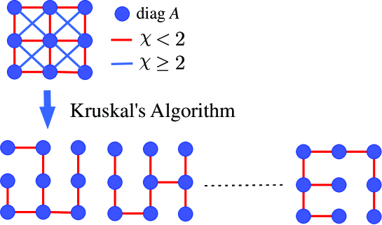
Figure 1: Image of Kruskal’s Algorithm

Let us focus on $l$-trees over $G$ whose root is a state $z^{l}\in{\rm diag}({\cal A})$. Recall now that the resistance of the tree is the sum of the weights of all the edges constituting the tree as defined in Subsection II-B. Then, we have the following lemma in terms of the stochastic potential of $z^{l}$, which is the minimal resistance among all $l$-trees in ${\cal G}(l)$.

Lemma 5

Consider the weighted directed graph $G$ constituted from the Markov process $\{P_{t}^{\varepsilon}\}$ induced by PHPIP applied to a constrained potential game $\Gamma$. Let us denote by ${\cal T}=({\rm diag}({\cal A}),{\cal E}_{l},{\cal W})$ the $l$-tree giving the stochastic potential of $z^{l}\in{\rm diag}({\cal A})$. If Assumptions 1 and 2 are satisfied, then the edge set ${\cal E}_{l}$ must be a subset of ${\cal E}_{single}$.

Proof

The edges of $G$, denoted by ${\cal E}$, are divided into two classes: ${\cal E}_{s}:={\cal E}_{single}$ and ${\cal E}_{d}:={\cal E}\setminus{\cal E}_{s}$. From Lemma 3, the weights of the edges in ${\cal E}_{s}$ are smaller than $2$. We next consider the weights of the edges in ${\cal E}_{d}$. Because of the nature of PHPIP, any agent cannot change his action to another one without explorations when $z(t)\in{\rm diag}({\cal A})$, and hence exploration should be executed more than twice in order that the transition along with an edge in ${\cal E}_{d}$ occurs. This implies that the weights of edges in ${\cal E}_{d}$ should be greater than $2$.

Hereafter, we simply rewrite the weights of the edges ${\cal E}_{s}$ by $w_{s}(<2)$ and those of ${\cal E}_{d}$ by $w_{d}(\geq 2)$ and build the minimal resistance tree with root $z^{l}$ over this simplified graph. Note that this simplification does not change the elements of the edge set ${\cal E}_{l}$. It should be noted that from Assumption 1 all recurrent communication classes (${\rm diag}({\mathcal{A}})$) can be connected by passing only through straight routes. From the procedure of Kruskal’s Algorithm, edges with resistances $w_{d}$ are never chosen as edges of the minimal tree as illustrated in Fig. 1. Thus, the tree giving the stochastic potential must consist only of the edges in ${\cal E}_{s}$, which completes the proof.

We are now ready to state the following proposition on the stochastically stable states (Definition 4) for the Markov process $\{P_{t}^{\varepsilon}\}$.

Proposition 3

Consider $\{P_{t}^{\varepsilon}\}$ induced by PHPIP applied to a constrained potential game $\Gamma$. If Assumptions 1 and 2 are satisfied, then the stochastically stable states are included in ${\rm diag}(\zeta(\Gamma))$, with the set of the optimal Nash equilibria $\zeta(\Gamma)$.

Proof

From Proposition 1, Lemmas 1 and 2, it is sufficient to prove that the states in ${\rm diag}({\cal A})$ with the minimal stochastic potential over $G$ are included in $\zeta(\Gamma)$.

Let us introduce the notations $z_{nonopt}=(a_{nonopt},a_{nonopt})\in{\rm diag}({\cal A})$ with a non optimal action $a_{nonopt}$ and $z_{opt}=(a_{opt},a_{opt})\in{\rm diag}({\mathcal{A}})$ with an optimal Nash equilibrium $a_{opt}$. If $z_{nonopt}$ is the root of a tree $T$, there exists a unique route from $z_{opt}$ to $z_{nonopt}$ over $T$. From Lemma 5, the route $r$ is an $m$-straight-route for some $m$. Now, we can build a tree $T^{\prime}$ with root $z_{opt}$ such that only the route $r$ is replaced by its reverse route $r^{\prime}$ (Fig. 2). Then, we have $\lambda(r)>\lambda(r^{\prime})$ from Lemma 4 since $\phi(a_{opt})>\phi(a_{nonopt})$. Thus, the resistance of $T^{\prime}$ is smaller than that of $T$ and the stochastic potential of $z_{opt}$ is smaller than the resistance of $T^{\prime}$. The statement holds regardless of the selection of $a_{nonopt}$. This completes the proof.

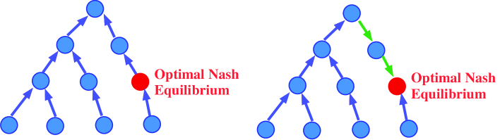
Figure 2: Resistance Trees (the left tree should have a greater resistance than the right)

We next consider PIPIP with time-varying $\varepsilon(t)$ and prove strong ergodicity of $\{P_{t}^{\varepsilon}\}$.

Lemma 6

The Markov process $\{P_{t}^{\varepsilon}\}$ induced by PIPIP applied to a constrained potential game $\Gamma$ is strongly ergodic.

Proof

We use Proposition 2 for the proof. Conditions (B2), (B3) in Proposition 2 can be proved in the same way as [7]. We thus show only the satisfaction of Condition (B1). As in (13), the probability of transition $z^{1}\rightarrow z^{2}$ is given by

$$P_{z^{1}z^{2}}^{\varepsilon} = \prod_{i\in\Lambda_{1}}\frac{\varepsilon}{|{\cal R}_{i}(a_{i}^{1})|-1}\times\prod_{i\in\Lambda_{2}}(1-\varepsilon)\times\prod_{i\in\Lambda_{3}}\frac{\varepsilon}{|{\cal R}_{i}(a_{i}^{1})|-h_{i}}\times$$ (23)

$$\times\prod_{i\in\Lambda_{4}}(1-\varepsilon)\kappa\varepsilon^{\Delta_{i}}\times\prod_{i\in\Lambda_{5}}(1-\varepsilon)(1-\kappa\varepsilon^{\Delta_{i}}).$$

Since $\varepsilon(t)$ is strictly decreasing, there is $t_{0}\geq 1$ such that $t_{0}$ is the first time when

$$(1-\varepsilon(t))(1-\kappa\varepsilon(t)^{\Delta_{i}})\geq\frac{\varepsilon(t)}{C-1},\ 1-\varepsilon(t)\geq\frac{\varepsilon(t)^{(1-\Delta_{i})}}{\kappa(C-1)}$$ (24)

holds. Note that the existence of $\varepsilon$ satisfying (24) is guaranteed from the condition (9). For all $t\geq t_{0}$, we have

$$P_{z^{1}z^{2}}^{\varepsilon}(t)\geq\left(\frac{\varepsilon(t)}{C-1}\right)^{n}.$$ (25)

The remaining part of the proof is the same as [7] and omit it in this paper.

We are now ready to prove Theorem 1. From Lemma 6, the distribution $\mu(\varepsilon(t))$ converges to the unique distribution $\mu^{*}$ from any initial state. In addition, we also have $\mu^{*}=\mu(0)={\lim}_{\varepsilon\rightarrow 0}\mu(\varepsilon)$ from ${\lim}_{t\rightarrow\infty}\varepsilon(t)=0$. We have already proved from Propositions 1 and 3 that any state $z$ satisfying $\mu_{z}(0)>0$ must be included in ${\rm diag}(\zeta(\Gamma))$. Therefore,

$${\lim}_{t\rightarrow\infty}{\rm Prob}[z(t)\in{\rm diag}(\zeta(\Gamma))]=1,$$

is proved, which completes the proof of Theorem 1. Theorem 2 is also proved from Proposition 1, Lemma 1 and Proposition 3.

V Application to Sensor Coverage Problem

In this section we demonstrate the effectiveness of the proposed learning algorithm PIPIP through experiments of the sensor coverage problem investigated e.g. in [3, 4, 5] whose objective is to cover a mission space efficiently using distributed control strategies. In particular, the problem of this section is formulated based on [7] with some modifications.

V-A Problem Formulation

We suppose that the mission space to be covered is given by ${\mathcal{Q}}^{c}\subset{\mathbb{R}}^{2}$ and that a density function $W^{c}(q),\ q\in{\mathcal{Q}}^{c}$ is defined over ${\mathcal{Q}}^{c}$. In particular, to constitute a game in the form of the previous sections, we also prepare a discretized mission space ${\mathcal{Q}}$ consisting of a finite number of points in ${\mathcal{Q}}^{c}$. Accordingly, we also define the discretized version of the density $W(q),\ q\in{\mathcal{Q}}$ such that $W(q)=W^{c}(q)\ {\forall q}\in{\mathcal{Q}}$.

In the problem, the position of agent $i$ in the mission space ${\mathcal{Q}}$ is regarded as the action $a_{i}$ to be determined, and hence the action set ${\cal A}_{i}$ is given by a subset of ${\mathcal{Q}}$ for all $i\in{{\cal V}}$. Namely, each agent $i$ chooses his action $a_{i}$ from the finite set ${\cal A}_{i}\subseteq{\mathcal{Q}}$ at each iteration and move toward the corresponding point.

Suppose now that each sensor has a limited sensing radius $r_{m}$ and that agent $i$ located at $a_{i}\in{\mathcal{Q}}$ may sense an event at $q\in{\mathcal{Q}}$ iff $q\in{\cal D}(a_{i}):=\{q\in{\mathcal{Q}}|\ \|q-a_{i}\|\leq r_{m}\}$. We also denote by $n_{q}(a)$ the number of agents such that $q\in{\cal D}(a_{i})$ when agents take the joint action $a$. Then, we define the function

$$\phi(a)=\sum_{q\in{\mathcal{Q}}}\sum^{n_{q}(a)}_{l=1}\frac{W(q)}{l}dq.$$

This function means, as $n_{q}(a)$ increases, the sensing accuracy at $q\in{\mathcal{Q}}$ improves but the increment decreases, which captures the characteristics of the sensor coverage problem. Note that the authors in [7] take account of energy consumption of sensors in addition to coverage performance and claim that the function $\phi$ cannot be a performance measure. However, we do not consider the energy consumption and what is the best selection of the performance measure depends on the subjective views of designers. We thus identify maximization of $\phi$ with the global objective of the group letting $\phi$ be the potential function.

Let us now introduce the utility function

$$U_{i}(a)=\sum_{q\in{\cal D}(a_{i})}\frac{W(q)}{n_{q}(a)}.$$

Then, equation (1) holds for the above potential function $\phi$ [7] and hence a potential game is constituted. It is also easy to confirm that the utility $U_{i}(a)$ can be locally computed if we assume feedbacks of $W_{q},\ q\in{\cal D}(a_{i})$ from environment and of the selected actions $a_{j},\ j\neq i$ only from neighboring agents specified by the $2r_{m}$-disk proximity communication graph [1].

V-B Objectives

In this section, we run two experiments whose objectives are listed below.

• Demonstration of effectiveness: Theorems 1 and 2 assure statements after infinitely long time but it is required in practice that the algorithm works in finite time. The first objective is thus to check if the agents successfully cover the mission space (i) even in the presence of constraints such as obstacles and mobility constraints, and (ii) in the absence of the prior information on the density function. The second objective is to compare its performance with the learning algorithm DISL, which is chosen to ensure fair comparisons. Indeed, the other existing algorithms require either or both of prior knowledge on density or free motion without constraints.

• Adaptability to environmental changes: In many real applications of sensor coverage schemes, it is required for sensors to change the configuration according to the surrounding environment. In particular, the density function can be time-varying e.g. in the scenario such as measuring of radiation quantity in the air and sampling of some chemical material and temperature in the ocean. It is expected for payoff-based algorithms to naturally adapt to such environmental changes without altering action selection rules and any complicated decision-making processes due to the characteristics that prior knowledge on environments except for ${\cal A}_{i}$ is not assumed. We thus check the function by using a Gaussian density function whose mean moves as time advances.

V-C Experimental System

Figure 3: Mobile Robot

In the experiments, we use four mobile robots with four wheels which can move in any direction (Fig. 3). Fig. 5 shows the schematic of the experimental system. A camera (Firefly MV (ViewPLUS Inc.) with lenses LTV2Z3314CS-IR (Raymax Inc.)) is mounted over the field. The image information is sent to a PC and processed to extract the pose of robots from the image by the image processing library OpenCV 2.0. Note that a board with two colored feature points is attached to each robot as in Fig. 3 to help the extraction. According to the extracted poses, the actions to be taken by agents are computed based on learning algorithms. However, in the experiments, the selected actions are not executed directly since collisions among robots must be avoided. For this purpose, a local decision-making mechanism checks whether collisions would occur if the selected actions were executed. The mechanism is designed based on heuristics and we avoid mentioning the details since it is not essential. If the answer of the mechanism is yes, the agents decide to stay at the current position. Otherwise, the selected actions are sent as reference positions together with the current poses to the local velocity and position PI controller implemented on a digital signal processor DS-1104 (dSPACE Inc.). Then, the eventual velocity command is sent to each robot via a wireless communication device XBee (Digi International Inc.).

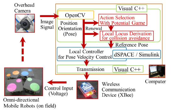
Figure 4: Experimental Schematic

Figure 5: Setting of Experiment 1

The following setup is common in all experiments. The mission space ${\mathcal{Q}}^{c}:=[0\ 2.7]{\rm m}\times[0\ 1.8]{\rm m}$ is divided into $9\times 6$ squares with side length $0.3$m as in Fig. 5 letting the discretized set ${\mathcal{Q}}$ be given by the centers of the squares as

$${\mathcal{Q}}=\{(0.15+0.3j,0.15+0.3l)|\ j\in\{0,\cdots,8\},\ l\in\{0,\cdots,5\}\}.$$

The sensing radius $r_{m}$ is set as $r_{m}=0.3$m for all robots. We also assume that each agent has a mobility constraint

$${\cal R}_{i}(a_{i})=\{a_{i}\pm 0.3(b_{1},b_{2})\in{\cal A}_{i}|\ b_{1}\in\{-1,0,1\},\ b_{2}\in\{-1,0,1\}\}.$$

The initial actions of agents are set as

$$a_{1}(0)=(0.15,0.15),\ a_{2}(0)=(0.15,0.45),\ a_{3}(0)=(0.45,0.15),\ a_{4}(0)=(0.45,0.45).$$

V-D Experiment 1

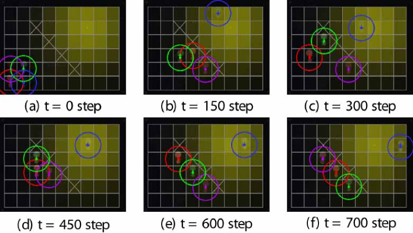
Figure 6: Configurations by DISL (Experiment 1)

In the first experiment, we demonstrate the effectiveness of PIPIP. For this purpose, we employ the density function

$$W(q)=e^{-\frac{25\|q-\mu\|^{2}}{9}},\ \mu=(1.95,1.35)$$

and prepare obstacles at

$${\mathcal{O}}:=\{(0.75,1.35),(1.05,1.05),(1.35,0.75),(1.65,0.45)\}.$$ (26)

Namely, in the experiment, the action sets are given by ${{\cal A}}_{i}={\mathcal{Q}}\setminus{\mathcal{O}}$. The setup is illustrated in Fig. 5, where the region with high density is colored by yellow and the red cross mark indicates the actions prohibited to be taken by the obstacles. Under the situation, we see that there exist some Nash undesirable equilibria just ahead on the left of the obstacles. It should be also noted that each robot does not know the function $W(q)$ a priori.

We first run DISL under the above situation with the exploration rate $\varepsilon=0.15$. Then, the resulting configurations at $0$, $150$, $300$, $450$, $600$ and $700$ steps are shown in Fig. 6. Under the setting, three robots cannot reach the colored region at least in $700$ step. It is now easily confirmed that the configurations at $600$ and $700$[step] are Nash equilibria only for the three robots and hence they cannot increase utilities by any one agent’s action change.

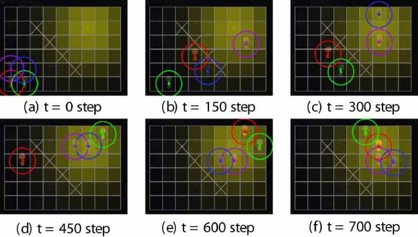
Figure 7: Configurations by PIPIP (Experiment 1)

We next run PIPIP letting the parameter $\varepsilon$ be fixed as $\varepsilon=0.15$ and setting $\kappa=0.5$ (namely, PHPIP is actually run in the experiment). Fig. 7 shows resulting configurations at the same steps as Fig. 6. Surprisingly, we see that all the robots eventually avoid the obstacles and arrive at the colored region though they initially do not know where is important. Such a behavior is never achieved by conventional coverage control schemes. The time responses of the potential function $\phi$ for PIPIP and DISL are illustrated in Fig. 9, where the solid line shows the response for PIPIP and the dashed line for DISL. As is apparent from the above investigations, PIPIP achieves a higher potential function value than DISL.

Though we can show only one sample due to the page constraints, similar results are obtained for both DISL and PIPIP through several trials. From the results, we claim that PIPIP has a stronger tendency to escape undesirable Nash equilibria than DISL, which is also confirmed by the meaning of the irrational decision. Of course, the results strongly depend on the value of exploration rate $\varepsilon$. We thus show the time evolution of the function $\phi$ for $\varepsilon=0.3$ in Fig. 9. We see from Fig. 9 that some agents executing DISL also do not reach the important region even for $\varepsilon=0.3$, which seems to be quite high probability as an exploration rate. Indeed, the fluctuation of the responses is large and an agent with PIPIP overcomes the obstacle again leaving the colored region. From all the above results, we thus can state that guarantees of only convergence to Nash equilibria can be a significant problem not only from the theoretical point of view but also from the practical viewpoint. Though much more thorough comparisons are necessary in order to make the claim on superiority of PIPIP over DISL confident, PIPIP achieves a better performance than DISL at least in the setup.

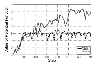
Figure 8: Time Evolution of Potential Function for $\varepsilon=0.15$ (Experiment 1)

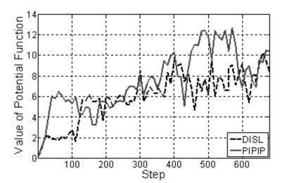
Figure 9: Time Evolution of Potential Function for $\varepsilon=0.3$ (Experiment 1)

V-E Experiment 2

We next demonstrate the adaptability of PIPIP to environmental changes, where we get rid of the obstacle ${\mathcal{O}}$ and hence ${\cal A}_{i}={\mathcal{Q}}$. In the experiment, we use the following Gaussian density function whose mean gradually moves.

$$W^{c}(q)=e^{-\frac{25\|q-\mu(t)\|^{2}}{9}},\ \mu(t)=\left\{\begin{array}[]{ll}(0.45,0.45),&\mbox{if }t\in[0,300]\\ (0.00375t-0.6750,0.00225t-0.225),&\mbox{if }t\in(300,700)\\ (1.95,1.35),&\mbox{if }t\geq 700\end{array}\right.$$ (30)

It is worth noting that agents select actions without using any prior information on the density.

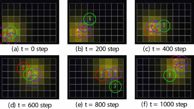
Figure 10: Configurations by PIPIP (Experiment 2)

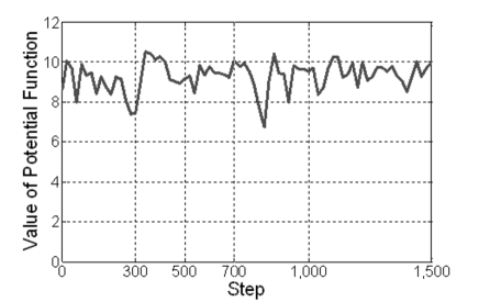
Figure 11: Time Evolution of Potential Function (Experiment 2)

Figs 10 and 11 respectively illustrate the resulting configurations at $0$, $200$, $400$, $600$, $800$ and $1000$ steps and time evolution of the potential function $\phi$. We see from Fig. 10 that agents gather at around the most important region at any time instant while learning the environmental changes. Fig. 11 also shows that the potential function keeps almost the same level during whole time, which indicates that the agents successfully track the most important region. From these results, as expected, agents executing PIPIP successfully adapt to the environmental changes without changing the action selection rule at all. Such a behavior is also never achieved by conventional coverage control schemes.

VI Conclusion

In this paper, we have developed a new learning algorithm Payoff-based Inhomogeneous Partially Irrational Play (PIPIP) for potential game theoretic cooperative control of multi-agent systems. The present algorithm is based on Distributed Inhomogeneous Synchronous Learning (DISL) presented in [7] and inherits several desirable features of DISL. However, unlike DISL, PIPIP allows agents to make irrational decisions, that is, take an action giving a lower utility from the past two actions. Thanks to the decision, we have succeeded proving convergence of the joint action to the potential function maximizers while escaping from undesirable Nash equilibria. Then, we have demonstrated the utility of PIPIP through experiments on a sensor coverage problem. It has been revealed through the demonstration that the present learning algorithm works even in a finite-time interval and agents successfully arrive at around the optimal Nash equilibria in the presence of obstacles in the mission space. In addition, we also have seen through an experiment with a moving density function that PIPIP has adaptability to environmental changes, which is a function expected for payoff-based learning algorithms.

References

- [1] F. Bullo, J. Cortes and S. Martinez, Distributed Control of Robotic Networks, Series in Applied Mathematics, Princeton University Press, 2009.
- [2] R. M. Murray, “Recent Research in Cooperative Control of Multivehicle Systems,” Journal of Dynamic Systems Measurement and Control-Transactions of The Asme, Vol. 129, No. 5, pp. 571–583, 2007.
- [3] J. Cortes, S.Martinez, T. Karatas and F. Bullo, “Coverage Control for Mobile Sensing Networks,” IEEE Trans. on Robotics and Automation, Vol. 20, No. 2, pp. 243–255, 2004.
- [4] W. Li and C. G. Cassandras, “Sensor Networks and Cooperative Control,” European Journal of Control, Vol. 11, pp. 436–463, 2005.
- [5] C. H. Caicedo-N and M. Zefran, “A Coverage Algorithm for A Class of Non-convex Regions,” in Proc. of the 47th IEEE International Conference on Decision and Control, pp. 4244–4249, 2008.
- [6] J. R. Marden, G. Arslan and J. S. Shamma, “Cooperative Control and Potential Games,” IEEE Trans. on Systems, Man and Cybernetics, Vol. 39, No. 6, pp. 1393–1407, 2009.
- [7] M. Zhu and S. Martinez, “Distributed Coverage Games for Mobile Visual Sensor Networks,” SIAM Journal on Control and Optimization, submitted (downloadable at arXiv:1002.0367v1), 2010.
- [8] N. Li and J. R. Marden, “Designing Games to Handle Coupled Constraints”, in Proc. of the 49th IEEE Conference on Decision and Control, pp. 250–255, 2010.
- [9] D. Monderer and L. Shapley, “Potential Games,” Games and Economic Behavior, Vol. 14, No. 1, pp. 124–143, 1996.
- [10] R. Gopalakrishnan, J. R. Marden and A. Wierman, “An Architectural View of Game Theoretic Control,” in Proc. of ACM Hotmetrics 2010: Third Workshop on Hot Topics in Measurement and Modeling of Computer Systems, 2010.
- [11] L. S. Shapley, A Value for -person Games, Contributions to the Theory of Games II, Princeton University Press, 1953.
- [12] D. Wolpert and K. Tumor, An Overview of Collective Intelligence, J. M. Bradshaw Eds. Handbook of Agent Technology, AAAI Press/MIT Press, 1999.
- [13] D. Monderer and L. Shapley, “Fictitious Play Property for Games with Identical Interests,” Journal of Economic Theory, Vol. 68, pp. 258–265 1996.
- [14] S. Hart and A. Mas-Colell, “Regret-based Continuous-time Dynamics,” Games and Economic Behavior, Vol. 45, No. 2, pp. 375–394, 2003.
- [15] J. R. Marden, G. Arslan and J. S. Shamma, “Joint Strategy Fictitious Play with Inertia for Potential Games,” IEEE Trans. on Automatic Control, Vol. 54, No. 2, pp. 208–220, 2009.
- [16] J. R. Marden, G. Arslan and J. S. Shamma, “Regret Based Dynamics: Convergence in Weakly Acyclic Games,” in Proc. of Sixth International Joint Conference on Autonomous Agents and Multi-Agent Systems, 2007.
- [17] H. P. Young, “The Evolution of Conventions,” Econometrica, Vol. 61, No. 1, pp. 57–84, 1993.
- [18] H. P. Young, Strategic Learning and Its Limits, Oxford University Press, 2004.
- [19] H. P. Young, Individual Strategy and Social Structure: An Evolutionary Theory of Institutions, Princeton University Press, 2001.
- [20] J. R. Marden, H. P. Young, G. Arslan and J. S. Shamma, “Payoff-based Dynamics for Multi-player Weakly Acyclic Games,” SIAM Journal on Control and Optimization, Vol. 48, No. 1, pp. 373–396, 2009.
- [21] J. R. Marden and J. S. Shamma, “Revisiting Log-linear Learning: Asynchrony, Completeness and Payoff-based Implementation,” Games and Economic Behavior, submitted, 2008.
- [22] G. Chasparis and J. Shamma, “Distributed Dynamic Reinforcement of Efficient Outcomes in Multiagent Coordination,” in Proc. of Third World Congress of the Game Theory Society, 2008.
- [23] D. Isaacson and R. Madsen, Markov Chains: Theory and Applications, New York, Wiley, 1976.