Analysis of a Fast Fourier Transform Based Method for Modeling of Heterogeneous Materials

Abstract

The focus of this paper is on the analysis of the Conjugate Gradient method applied to a non-symmetric system of linear equations, arising from a Fast Fourier Transform-based homogenization method due to Moulinec and Suquet [1]. Convergence of the method is proven by exploiting a certain projection operator reflecting physics of the underlying problem. These results are supported by a numerical example, demonstrating significant improvement of the Conjugate Gradient-based scheme over the original Moulinec-Suquet algorithm.

1 Introduction

The last decade has witnessed a rapid development in advanced experimental techniques and modeling tools for microstructural characterization, typically provided in the form of pixel- or voxel-based geometry. Such data now allow for the design of bottom-up predictive models of the overall behavior for a wide range of engineering materials. Of course, such step necessitates the development of specialized algorithms, capable of handling large-scale voxel-based data in an efficient manner. In the engineering community, perhaps the most successful solver meeting these criteria was proposed by Moulinec and Suquet in [1]. The algorithm is based on the Neumann series expansion of the inverse of an operator arising in the associated Lippmann-Schwinger equation and exploits the Fast Fourier Transform to evaluate the action of the operator efficiently for voxel-based data. In our recent work [2], we have offered a new approach to the Moulinec-Suquet scheme, by exploiting the trigonometric collocation method due to Saranen and Vainikko [3]. Here, the Lippman-Schwinger equation is projected to a space of trigonometric polynomials to yield a non-symmetric system of linear equations, see Section 2 below. Quite surprisingly, numerical experiments revealed that the system can be efficiently solved using the standard Conjugate Gradient algorithm. The analysis of this phenomenon, as presented in Section 3, is at the heart of this contribution. The obtained results are further supported by a numerical example in Section 4 and summarized in Section 5.

The following notation is used throughout the paper. Symbols $a$, $\boldsymbol{a}$ and $\boldsymbol{A}$ denote scalar, vector and second-order tensor quantities, respectively, with Greek subscripts used when referring to the corresponding components, e.g. $A_{\alpha\beta}$. The outer product of two vectors is denoted as $\boldsymbol{a}\otimes\boldsymbol{a}$, whereas $\boldsymbol{a}\cdot\boldsymbol{b}$ or $\boldsymbol{A}\cdot\boldsymbol{b}$ represents the single contraction between vectors (or tensors). A multi-index notation is employed, in which $\mathbb{R}^{{\boldsymbol{N}}}$ with ${\boldsymbol{N}}=(N_{1},\ldots,N_{d})$ represents $\mathbb{R}^{N_{1}\times\cdots\times N_{d}}$ and $|{\boldsymbol{N}}|$ abbreviates $\prod_{\alpha=1}^{d}N_{\alpha}$. Block matrices are denoted by capital letters typeset in a bold serif font, e.g. $\boldsymbol{\mathsf{A}}\in\mathbb{R}^{d\times d\times{\boldsymbol{N}}\times{\boldsymbol{N}}}$, and the superscript and subscript indexes are used to refer to the components, such that $\boldsymbol{\mathsf{A}}=[\mathsf{A}^{\boldsymbol{k}\boldsymbol{m}}_{\alpha\beta}]_{\alpha,\beta=1,\dotsc,d}^{\boldsymbol{k},\boldsymbol{m}\in\widebar{\mathbb{Z}}^{{\boldsymbol{N}}}}$ with

$$\widebar{\mathbb{Z}}^{{\boldsymbol{N}}}=\left\{\boldsymbol{k}\in\mathbb{Z}^{d}:-\frac{N_{\alpha}}{2}<k_{\alpha}\leq\frac{N_{\alpha}}{2},\alpha=1,\ldots,d\right\}.$$

Sub-matrices of $\boldsymbol{\mathsf{A}}$ are denoted as

$$\boldsymbol{\mathsf{A}}_{\alpha\beta}=\left[\mathsf{A}_{\alpha\beta}^{\boldsymbol{k}\boldsymbol{m}}\right]^{\boldsymbol{k},\boldsymbol{m}\in\widebar{\mathbb{Z}}^{{\boldsymbol{N}}}}\in\mathbb{R}^{{\boldsymbol{N}}\times{\boldsymbol{N}}}, \boldsymbol{\mathsf{A}}^{\boldsymbol{k}\boldsymbol{m}}=\left[\mathsf{A}_{\alpha\beta}^{\boldsymbol{k}\boldsymbol{m}}\right]_{\alpha,\beta=1,\dotsc,d}\in\mathbb{R}^{d\times d}$$

for $\alpha,\beta=1,\dotsc,d$ and $\boldsymbol{k},\boldsymbol{m}\in\widebar{\mathbb{Z}}^{{\boldsymbol{N}}}$. Analogously, the block vectors are denoted by lower case letters, e.g. $\boldsymbol{\mathsf{e}}\in\mathbb{R}^{d\times{\boldsymbol{N}}}$ and the matrix-by-vector multiplication is defined as

$$\left[\mathsf{A}\mathsf{e}\right]_{\alpha}^{\boldsymbol{k}}=\sum_{\beta=1}^{d}\sum_{\boldsymbol{m}\in\widebar{\mathbb{Z}}^{{\boldsymbol{N}}}}\mathsf{A}_{\alpha\beta}^{\boldsymbol{k}\boldsymbol{m}}\mathsf{e}_{\beta}^{\boldsymbol{m}}\in\mathbb{R}^{d\times{\boldsymbol{N}}},$$ (1)

with $\alpha=1,\dotsc,d$ and $\boldsymbol{k}\in\widebar{\mathbb{Z}}^{{\boldsymbol{N}}}$.

2 Problem setting

Consider a composite material represented by a periodic unit cell

$$\mathcal{Y}=\prod_{\alpha=1}^{d}(-Y_{\alpha},Y_{\alpha})\subset\mathbb{R}^{d}.$$

In the context of linear electrostatics, the associated unit cell problem reads as

$$\boldsymbol{\nabla}\times\boldsymbol{e}(\boldsymbol{x}) ={\boldsymbol{0}}, \boldsymbol{\nabla}\cdot\boldsymbol{j}(\boldsymbol{x}) ={\boldsymbol{0}}, \boldsymbol{j}(\boldsymbol{x}) =\boldsymbol{L}(\boldsymbol{x})\cdot\boldsymbol{e}(\boldsymbol{x}), \boldsymbol{x} \in\mathcal{Y}$$ (2)

where $\boldsymbol{e}$ is a $\mathcal{Y}$-periodic vectorial electric field, $\boldsymbol{j}$ denotes the corresponding vector of electric current and $\boldsymbol{L}$ is a second-order positive-definite tensor of electric conductivity. In addition, the field $\boldsymbol{e}$ is subject to a constraint

$$\langle\boldsymbol{e}(\boldsymbol{x})\rangle:=\frac{1}{\left\lvert\mathcal{Y}\right\rvert}\int_{\mathcal{Y}}\boldsymbol{e}(\boldsymbol{x})\operatorname{d\!}{\boldsymbol{x}}=\boldsymbol{e}^{0},$$ (3)

where $\left\lvert\mathcal{Y}\right\rvert$ denotes the $d$-dimensional measure of $\mathcal{Y}$ and $\boldsymbol{e}^{0}\neq\boldsymbol{0}$ a prescribed macroscopic electric field.

The original problem (2)–(3) is then equivalent to the periodic Lippmann-Schwinger integral equation, formally written as

$$\boldsymbol{e}(\boldsymbol{x})+\int_{\mathcal{Y}}{\boldsymbol{\Gamma}}(\boldsymbol{x}-\boldsymbol{y};\boldsymbol{L}^{0})\cdot\Bigl{(}\boldsymbol{L}(\boldsymbol{y})-\boldsymbol{L}^{0}\Bigr{)}\cdot\boldsymbol{e}(\boldsymbol{y})\operatorname{d\!}{\boldsymbol{y}}=\boldsymbol{e}^{0},\quad\boldsymbol{x}\in\mathcal{Y},$$ (4)

where $\boldsymbol{L}^{0}\in\mathbb{R}^{d\times d}$ denotes a homogeneous reference medium. The operator ${\boldsymbol{\Gamma}}(\boldsymbol{x},\boldsymbol{L}^{0})$ is derived from the Green’s function of the problem (2)–(3) with $\boldsymbol{L}(\boldsymbol{x})=\boldsymbol{L}^{0}$ and can be simply expressed in the Fourier space

$${\boldsymbol{\hat{\Gamma}}}(\boldsymbol{k};\boldsymbol{L}^{0})=\begin{cases}{\boldsymbol{0}}&\boldsymbol{k}={\boldsymbol{0}}\\ \displaystyle\frac{\boldsymbol{\xi}\otimes\boldsymbol{\xi}}{\boldsymbol{\xi}\cdot\boldsymbol{L}^{0}\cdot\boldsymbol{\xi}}&\boldsymbol{\xi}(\boldsymbol{k})=\left(\frac{k_{\alpha}}{Y_{\alpha}}\right)_{\alpha=1}^{d};\boldsymbol{k}\in\mathbb{Z}^{d}\setminus{\boldsymbol{0}}.\end{cases}$$ (5)

Operator $\widehat{f}=\widehat{f}(\boldsymbol{k})$ stands for the Fourier coefficient of $f(\boldsymbol{x})$ for the $\boldsymbol{k}$-th frequency given by

$$\widehat{f}(\boldsymbol{k})=\int_{\mathcal{Y}}f(\boldsymbol{x})\varphi_{-\boldsymbol{k}}(\boldsymbol{x})\operatorname{d\!}{x}, \varphi_{\boldsymbol{k}}(\boldsymbol{x})=|\mathcal{Y}|^{-\frac{1}{2}}\exp\left(\mathrm{i}\pi\sum_{\alpha=1}^{d}\frac{x_{\alpha}k_{\alpha}}{Y_{\alpha}}\right),$$ (6)

”$\mathrm{i}$” is the imaginary unit ($\mathrm{i}^{2}=-1$). We refer to [2, 4] for additional details. Note that the linear electrostatics serves here as a model problem; the framework can be directly extended to e.g. elasticity [5], (visco-)plasticity [6] or to multiferroics [7].

2.1 Discretization via trigonometric collocation

The numerical solution of the Lippmann-Schwinger equation is based on a discretization of a unit cell $\mathcal{Y}$ into a regular periodic grid with $N_{1}\times\cdots\times N_{d}$ nodal points and grid spacings $\boldsymbol{h}=(2Y_{1}/N_{1},\ldots,2Y_{d}/N_{d})$. The searched field $\boldsymbol{e}$ in (4) is approximated by a trigonometric polynomial $\boldsymbol{e}^{\boldsymbol{N}}$ in the form (cf. [3, Chapter 10])

$$\boldsymbol{e}(\boldsymbol{x})\approx\boldsymbol{e}^{\boldsymbol{N}}(\boldsymbol{x})=\sum_{\boldsymbol{\boldsymbol{k}}\in\widebar{\mathbb{Z}}^{{\boldsymbol{N}}}}\hat{\boldsymbol{\mathsf{e}}}^{\boldsymbol{k}}\varphi_{\boldsymbol{k}}(\boldsymbol{x}), \boldsymbol{x}\in\mathcal{Y},$$ (7)

where $\hat{\boldsymbol{\mathsf{e}}}^{\boldsymbol{k}}=(\hat{\mathsf{e}}^{\boldsymbol{k}}_{\alpha})_{\alpha=1,\dotsc,d}$ designates the Fourier coefficients defined in (6). Notice that the trigonometrical polynomials are uniquely determined by a regular grid data, which makes them well-suited to problems with pixel- or voxel-based computations.

The trigonometric collocation method is based on the projection of the Lippmann-Schwinger equation (4) onto the space of the trigonometric polynomials

$$\mathcal{T}^{\boldsymbol{N}}=\Bigl{\{}\sum_{{\boldsymbol{k}}\in\widebar{\mathbb{Z}}^{{\boldsymbol{N}}}}c_{\boldsymbol{k}}\varphi_{\boldsymbol{k}},c_{\boldsymbol{k}}\in\mathbb{C}\Bigr{\}},$$ (8)

leading to a to linear system in the form, cf. [2]

$$({\boldsymbol{\mathsf{I}}}+{\boldsymbol{\mathsf{B}}})\boldsymbol{\mathsf{e}}=\boldsymbol{\mathsf{e^{0}}}, {\boldsymbol{\mathsf{B}}}=\boldsymbol{\mathsf{F}}^{-1}{\boldsymbol{\mathsf{\hat{\Gamma}}}}\boldsymbol{\mathsf{F}}(\boldsymbol{\mathsf{L}}-\boldsymbol{\mathsf{L^{0}}}),$$ (9)

where $\boldsymbol{\mathsf{e}}=\left(\mathsf{e}_{\alpha}^{\boldsymbol{k}}\right)_{\alpha=1,\dotsc,d}^{\boldsymbol{k}\in\widebar{\mathbb{Z}}^{{\boldsymbol{N}}}}\in\mathbb{R}^{d\times{\boldsymbol{N}}}$ is the unknown vector, ${\boldsymbol{\mathsf{I}}}=\left[\delta_{\alpha\beta}\delta_{\boldsymbol{k}\boldsymbol{m}}\right]_{\alpha,\beta=1,\dotsc,d}^{\boldsymbol{k}\boldsymbol{m}\in\widebar{\mathbb{Z}}^{{\boldsymbol{N}}}}\in\mathbb{R}^{d\times d\times{\boldsymbol{N}}\times{\boldsymbol{N}}}$ is the identity matrix, expressed as the product of the Kronecker delta functions $\delta_{\alpha\beta}$ and $\delta_{\boldsymbol{k}\boldsymbol{m}}$, and $\boldsymbol{\mathsf{e^{0}}}=(e^{0}_{\alpha})_{\alpha=1,\dotsc,d}^{\boldsymbol{k}\in\widebar{\mathbb{Z}}^{{\boldsymbol{N}}}}\in\mathbb{R}^{d\times{\boldsymbol{N}}}$.

All the matrices in (9) exhibit a block-diagonal structure. In particular,

$${\boldsymbol{\mathsf{\hat{\Gamma}}}}=\left[\delta_{\boldsymbol{k}\boldsymbol{m}}{\mathsf{\hat{\Gamma}}}_{\alpha\beta}^{\boldsymbol{k}\boldsymbol{m}}\right]_{\alpha,\beta=1,\dotsc,d}^{\boldsymbol{k},\boldsymbol{m}\in\widebar{\mathbb{Z}}^{{\boldsymbol{N}}}}, \displaystyle\boldsymbol{\mathsf{L}}=\left[\delta_{\boldsymbol{k}\boldsymbol{m}}\mathsf{L}_{\alpha\beta}^{\boldsymbol{k}\boldsymbol{m}}\right]_{\alpha,\beta=1,\dotsc,d}^{\boldsymbol{k},\boldsymbol{m}\in\widebar{\mathbb{Z}}^{{\boldsymbol{N}}}}, \boldsymbol{\mathsf{L^{0}}}=\left[\delta_{\boldsymbol{k}\boldsymbol{m}}\mathsf{L^{0}}_{\alpha\beta}\right]_{\alpha,\beta=1,\dotsc,d}^{\boldsymbol{k},\boldsymbol{m}\in\widebar{\mathbb{Z}}^{{\boldsymbol{N}}}},$$

with ${\mathsf{\hat{\Gamma}}}_{\alpha\beta}^{\boldsymbol{k}\boldsymbol{k}}={\hat{\Gamma}}_{\alpha\beta}(\boldsymbol{k};\boldsymbol{L}^{0})$, $\mathsf{L}_{\alpha\beta}^{\boldsymbol{k}\boldsymbol{k}}=L_{\alpha\beta}(\boldsymbol{k})$ and $(\mathsf{L^{0}})_{\alpha\beta}=L^{0}_{\alpha\beta}$. The matrix $\boldsymbol{\mathsf{F}}$ implements the Discrete Fourier Transform and is defined as

$$\boldsymbol{\mathsf{F}} =\left[\delta_{\alpha\beta}\mathsf{F}^{\boldsymbol{k}\boldsymbol{m}}\right]_{\alpha,\beta=1,\dotsc,d}^{\boldsymbol{k},\boldsymbol{m}\in\widebar{\mathbb{Z}}^{{\boldsymbol{N}}}}, \mathsf{F}^{\boldsymbol{k}\boldsymbol{m}} =\frac{|\mathcal{Y}|^{\frac{1}{2}}}{\prod_{\alpha=1}^{d}N_{\alpha}}\exp\left(-\sum_{\alpha=1}^{d}2\pi\mathrm{i}\frac{k_{\alpha}m_{\alpha}}{N_{\alpha}}\right),$$ (10)

with $\boldsymbol{\mathsf{F}}^{-1}$ representing the inverse transform.

It follows from Eq. (1) that the cost of multiplication by ${\boldsymbol{\mathsf{B}}}$ is dominated by the action of $\boldsymbol{\mathsf{F}}$ and $\boldsymbol{\mathsf{F}}^{-1}$, which can be performed in $O(\left\lvert{\boldsymbol{N}}\right\rvert\log\left\lvert{\boldsymbol{N}}\right\rvert)$ operations by the Fast Fourier Transform techniques. This makes the system (9) well-suited for applying some iterative solution technique. In particular, the original Fast Fourier Transform-based Homogenization scheme formulated by Moulinec and Suquet in [1] is based on the Neumann expansion of the matrix inverse $(\boldsymbol{\mathsf{I}}+\boldsymbol{\mathsf{B}})^{-1}$, so as to yield the $m$-th iterate in the form

$$\boldsymbol{\mathsf{e}}^{(m)}=\sum_{j=0}^{m}\left(-\boldsymbol{\mathsf{B}}\right)^{j}\boldsymbol{\mathsf{e^{0}}}.$$ (11)

As indicated earlier, our numerical experiments [2] suggest that the system can be efficiently solved using the Conjugate Gradient method, despite the non-symmetry of ${\boldsymbol{\mathsf{B}}}$ evident from (9). This observation is studied in more detail in the next Section.

3 Solution by the Conjugate Gradient method

We start our analysis with recasting the system (9) into a more convenient form, by employing a certain operator and the associated sub-space introduced later. Note that for simplicity, the reference conductivity is taken as $\boldsymbol{\mathsf{L^{0}}}=\lambda{\boldsymbol{\mathsf{I}}}$.

Definition 1

Given $\lambda>0$, we define operator $\boldsymbol{\mathsf{P}}_{\mathcal{E}}=\lambda\boldsymbol{\mathsf{F}}^{-1}{\boldsymbol{\mathsf{\hat{\Gamma}}}}\boldsymbol{\mathsf{F}}$ and associated sub-space as

$$\mathcal{E}=\left\{\boldsymbol{\mathsf{P}}_{\mathcal{E}}\boldsymbol{\mathsf{x}}\mathrm{~{}for~{}}\boldsymbol{\mathsf{x}}\in\mathbb{R}^{d\times{\boldsymbol{N}}}\right\}\subset\mathbb{R}^{d\times{\boldsymbol{N}}}.$$

Lemma 1

The operator $\boldsymbol{\mathsf{P}}_{\mathcal{E}}$ is an orthogonal projection.

Proof

First, we will prove that $\boldsymbol{\mathsf{P}}_{\mathcal{E}}$ is projection, i.e. $\boldsymbol{\mathsf{P}}_{\mathcal{E}}^{2}=\boldsymbol{\mathsf{P}}_{\mathcal{E}}$. Since $\boldsymbol{\mathsf{F}}$ is a unitary matrix, it is easy to see that

$$\boldsymbol{\mathsf{P}}_{\mathcal{E}}^{2}=(\lambda\boldsymbol{\mathsf{F}}^{-1}\boldsymbol{\mathsf{{\hat{\Gamma}}}}\boldsymbol{\mathsf{F}})(\lambda\boldsymbol{\mathsf{F}}^{-1}\boldsymbol{\mathsf{{\hat{\Gamma}}}}\boldsymbol{\mathsf{F}})=\boldsymbol{\mathsf{F}}^{-1}(\lambda{\boldsymbol{\mathsf{\hat{\Gamma}}}})^{2}\boldsymbol{\mathsf{F}}.$$ (12)

Hence, in view of the block-diagonal character of $\boldsymbol{\mathsf{{\hat{\Gamma}}}}$, it it sufficient to prove the projection property of sub-matrices $(\lambda{\boldsymbol{\mathsf{\hat{\Gamma}}}})^{\boldsymbol{k}\boldsymbol{k}}$ only. This follows using a simple algebra, recall Eq. (5):

$$(\lambda{\boldsymbol{\mathsf{\hat{\Gamma}}}})^{\boldsymbol{k}\boldsymbol{k}}(\lambda{\boldsymbol{\mathsf{\hat{\Gamma}}}})^{\boldsymbol{k}\boldsymbol{k}}=\frac{\boldsymbol{\xi}(\boldsymbol{k})\otimes\boldsymbol{\xi}(\boldsymbol{k})}{\boldsymbol{\xi}(\boldsymbol{k})\cdot\boldsymbol{\xi}(\boldsymbol{k})}\cdot\frac{\boldsymbol{\xi}(\boldsymbol{k})\otimes\boldsymbol{\xi}(\boldsymbol{k})}{\boldsymbol{\xi}(\boldsymbol{k})\cdot\boldsymbol{\xi}(\boldsymbol{k})}=\frac{\boldsymbol{\xi}(\boldsymbol{k})\otimes\boldsymbol{\xi}(\boldsymbol{k})}{\boldsymbol{\xi}(\boldsymbol{k})\cdot\boldsymbol{\xi}(\boldsymbol{k})}=(\lambda{\boldsymbol{\mathsf{\hat{\Gamma}}}})^{\boldsymbol{k}\boldsymbol{k}}.$$

The orthogonality of $\boldsymbol{\mathsf{P}}_{\mathcal{E}}$ now follows from

$$\boldsymbol{\mathsf{P}}_{\mathcal{E}}^{*}=\left(\lambda\boldsymbol{\mathsf{F}}^{-1}{\boldsymbol{\mathsf{\hat{\Gamma}}}}\boldsymbol{\mathsf{F}}\right)^{*}=\lambda\boldsymbol{\mathsf{F}}^{*}{\boldsymbol{\mathsf{\hat{\Gamma}}}}^{*}\left(\boldsymbol{\mathsf{F}}^{-1}\right)^{*}=\lambda\boldsymbol{\mathsf{F}}^{-1}{\boldsymbol{\mathsf{\hat{\Gamma}}}}\boldsymbol{\mathsf{F}}=\boldsymbol{\mathsf{P}}_{\mathcal{E}},$$

according to a well-known result of linear algebra, e.g. Proposition 1.8 in [8]. ∎

Remark 1

It follows from the previous results that the subspace $\mathcal{E}$ collects the non-zero coefficients of trigonometric polynomials $\mathcal{T}^{\boldsymbol{N}}$ with zero rotation, which represent admissible solutions to the unit cell problem defined by (2). Note that the orthogonal space $\mathcal{E^{\perp}}$ contains the trigonometric representation of constant fields, cf. [4, Section 12.7].

Lemma 2

The solution $\boldsymbol{\mathsf{e}}$ to the linear system (9) admits the decomposition $\boldsymbol{\mathsf{e}}=\boldsymbol{\mathsf{e^{0}}}+\boldsymbol{\mathsf{e}}_{\mathcal{E}}$, with $\boldsymbol{\mathsf{e}}_{\mathcal{E}}\in\mathcal{E}$ satisfying

$$\boldsymbol{\mathsf{P}}_{\mathcal{E}}\boldsymbol{\mathsf{L}}\boldsymbol{\mathsf{e}}_{\mathcal{E}}+\boldsymbol{\mathsf{P}}_{\mathcal{E}}\boldsymbol{\mathsf{L}}\boldsymbol{\mathsf{e^{0}}}=\boldsymbol{\mathsf{0}}.$$ (13)

Proof

As $\boldsymbol{\mathsf{e}}\in\mathbb{R}^{d\times{\boldsymbol{N}}}$, Lemma 1 ensures that it can be decomposed into two orthogonal parts $\boldsymbol{\mathsf{e}}_{\mathcal{E}}=\boldsymbol{\mathsf{P}}_{\mathcal{E}}\boldsymbol{\mathsf{e}}$ and $\boldsymbol{\mathsf{e}}_{\mathcal{E^{\perp}}}=({\boldsymbol{\mathsf{I}}}-\boldsymbol{\mathsf{P}}_{\mathcal{E}})\boldsymbol{\mathsf{e}}$. Substituting this expression into (9), and using the identity $\boldsymbol{\mathsf{B}}=\lambda\boldsymbol{\mathsf{F}}^{-1}{\boldsymbol{\mathsf{\hat{\Gamma}}}}\boldsymbol{\mathsf{F}}\left(\tfrac{\boldsymbol{\mathsf{L}}}{\lambda}-\boldsymbol{\mathsf{I}}\right)$, we arrive at

$$\frac{1}{\lambda}\boldsymbol{\mathsf{P}}_{\mathcal{E}}\boldsymbol{\mathsf{L}}\boldsymbol{\mathsf{e}}_{\mathcal{E}}+\boldsymbol{\mathsf{e}}_{\mathcal{E^{\perp}}}+\frac{1}{\lambda}\boldsymbol{\mathsf{P}}_{\mathcal{E}}\boldsymbol{\mathsf{L}}\boldsymbol{\mathsf{e}}_{\mathcal{E^{\perp}}}=\boldsymbol{\mathsf{e^{0}}}.$$ (14)

Since $\boldsymbol{\mathsf{e}}^{0}\in\mathcal{E^{\perp}}$, we have $\boldsymbol{\mathsf{e}}_{\mathcal{E^{\perp}}}=\boldsymbol{\mathsf{e^{0}}}$ and the proof is complete. ∎

With these auxiliary results in hand, we are in the position to present our main result.

Proposition 1

The non-symmetric system of linear equations (9) is solvable by the Conjugate Gradient method for an initial vector $\boldsymbol{\mathsf{e}}_{(0)}=\boldsymbol{\mathsf{e}}^{0}+\widetilde{\boldsymbol{\mathsf{e}}}$ with $\widetilde{\boldsymbol{\mathsf{e}}}\in\mathcal{E}$. Moreover, the sequence of iterates is independent of the parameter $\lambda$.

Proof (outline)

It follows from Lemma 2 that the solution to (9) admits yet another, optimization-based, characterization in the form

$$\boldsymbol{\mathsf{e}}=\boldsymbol{\mathsf{e}}^{0}+\arg\min_{\bar{\boldsymbol{\mathsf{e}}}\in\mathcal{E}}\left[\frac{1}{2}\bigl{(}\boldsymbol{\mathsf{L}}\bar{\boldsymbol{\mathsf{e}}},\bar{\boldsymbol{\mathsf{e}}}\bigr{)}_{\mathbb{R}^{d\times{\boldsymbol{N}}}}+\bigl{(}\boldsymbol{\mathsf{L}}\boldsymbol{\mathsf{e}}^{0},\bar{\boldsymbol{\mathsf{e}}}\bigr{)}_{\mathbb{R}^{d\times{\boldsymbol{N}}}}\right].$$ (15)

The residual corresponding to the initial vector $\boldsymbol{\mathsf{e}}_{(0)}$ equals to

$$\boldsymbol{\mathsf{r}}_{(0)}=\boldsymbol{\mathsf{e}}^{0}-\left({\boldsymbol{\mathsf{I}}}+{\boldsymbol{\mathsf{B}}}\right)\left(\boldsymbol{\mathsf{e}}^{0}+\widetilde{\boldsymbol{\mathsf{e}}}\right)=-\frac{1}{\lambda}\boldsymbol{\mathsf{P}}_{\mathcal{E}}\boldsymbol{\mathsf{L}}\boldsymbol{\mathsf{e}}^{0}-\frac{1}{\lambda}\boldsymbol{\mathsf{P}}_{\mathcal{E}}\boldsymbol{\mathsf{L}}\widetilde{\boldsymbol{\mathsf{e}}}\in\mathcal{E}.$$

It can be verified that the subspace $\mathcal{E}$ is ${\boldsymbol{\mathsf{B}}}$-invariant, thus $({\boldsymbol{\mathsf{I}}}+{\boldsymbol{\mathsf{B}}})\mathcal{E}\subset\mathcal{E}$. Therefore, the Krylov subspace

$$\mathscr{K}_{m}({\boldsymbol{\mathsf{I}}}+{\boldsymbol{\mathsf{B}}},\boldsymbol{\mathsf{r}}_{(0)})=\mathrm{span}\left\{\boldsymbol{r}_{(0)},({\boldsymbol{\mathsf{I}}}+{\boldsymbol{\mathsf{B}}})\boldsymbol{\mathsf{r}}_{(0)},\ldots,({\boldsymbol{\mathsf{I}}}+{\boldsymbol{\mathsf{B}}})^{m}\boldsymbol{\mathsf{r}}_{(0)}\right\}\subset\mathcal{E}$$

for arbitrary $m\in\mathbb{N}$. This implies that the residual $\boldsymbol{\mathsf{r}}_{(m)}$ and the Conjugate Gradient search direction $\boldsymbol{\mathsf{p}}_{(m)}$ at the $m$-th iteration satisfy $\boldsymbol{\mathsf{r}}_{(m)}\in\mathcal{E}$ and $\boldsymbol{\mathsf{p}}_{(m)}\in\mathcal{E}$. Since ${\boldsymbol{\mathsf{B}}}$ is symmetric and positive-definite on $\mathcal{E}$, the convergence of $\mathrm{CG}$ algorithm now follows from standard arguments, e.g. Theorem 6.6 in [8]. Observe that different choices of $\lambda$ generate identical Krylov subspaces, thus the sequence of iterates is independent of $\lambda$.∎

Remark 2

Note that it is possible to show, using direct calculations based on the projection properties of $\boldsymbol{\mathsf{P}}_{\mathcal{E}}$, that the Biconjugate Gradient algorithm produces exactly the same sequence of vectors as the Conjugate Gradient method, see  [9].

4 Numerical example

To support our theoretical results, we consider a three-dimensional model problem of electric conduction in a cubic periodic unit cell $\mathcal{Y}=\prod_{\alpha=1}^{3}(-\frac{1}{2},\frac{1}{2})$, representing a two-phase medium with spherical inclusions of $25\%$ volume fraction. The conductivity parameters are defined as

$$\boldsymbol{L}(\boldsymbol{x})=\begin{cases}\rho\boldsymbol{I},&\|\boldsymbol{x}\|_{2}<(\frac{3}{16\pi})^{\frac{1}{3}}\\ \begin{pmatrix}1&0.2&0.2\\ 0.2&1&0.2\\ 0.2&0.2&1\\ \end{pmatrix},&\text{otherwise}\end{cases}$$

where $\rho>0$ denotes the contrast of phase conductivities. We consider the macroscopic field $\boldsymbol{e}^{0}=[1,0,0]$ and discretize the unit cell with ${\boldsymbol{N}}=[n,n,n]$ nodes. The conductivity of the homogeneous reference medium $\boldsymbol{L}^{0}\in\mathbb{R}^{d\times d}$ is parametrized as

$$\boldsymbol{L}^{0} =\lambda\boldsymbol{I}, \lambda =1-\omega+\rho\omega,$$ (16)

where $\omega\approx 0.5$ delivers the optimal convergence of the original Moulinec-Suquet Fast-Fourier Transform-based Homogenization ($\mathrm{FFTH}$) algorithm [1].

We first investigate the sensitivity of Conjugate Gradient ($\mathrm{CG}$) algorithm to the choice of reference medium. The results appear in Fig. 1, plotting the relative number of iterations for $\mathrm{CG}$ against the conductivity of the reference medium parametrized by $\omega$, recall Eq. (16). As expected, $\mathrm{CG}$ solver achieve a significant improvement over $\mathrm{FFTH}$ method as it requires about $40\%$ iterations of $\mathrm{FFTH}$ for a mildly-contrasted composite down to $4\%$ for $\varrho=10^{3}$. The minor differences visible especially for $\rho=10^{3}$ can be therefore attributed to accumulation of round-off errors. These observations fully confirm our theoretical results presented earlier in Section 3.

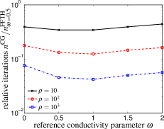
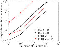
Figure 1: (a) Relative number of iterations as a function of the reference medium parameter $\omega$ and (b) computational time as a function of the number of unknowns.

In Fig. 1, we present the total computational time as a function of the number of degrees of freedom and the phase ratio $\rho$. The results confirm that the computational times scales linearly with the increasing number of degrees of freedom for both schemes for a fixed $\rho$ [2]. The ratio of the computational time for CG and FFTH algorithms remains almost constant, which indicates that the cost of a single iteration of $\mathrm{CG}$ and $\mathrm{FFTH}$ method is comparable.

In addition, the memory requirements of both schemes are also comparable. This aspect represents the major advantage of the short-recurrence CG-based scheme over alternative schemes for non-symmetric systems, such as GMRES. Finally note that finer discretizations can be treated by a straightforward parallel implementation.

5 Conclusions

In this work, we have proven the convergence of Conjugate Gradient method for a non-symmetric system of linear equations arising from periodic unit cell homogenization problem and confirmed it by numerical experiment. The important conclusions to be pointed out are as follows:

1. The success of the Conjugate Gradient method follows from the projection properties of operator $\boldsymbol{\mathsf{P}}_{\mathcal{E}}$ introduced in Definition 1, which reflect the structure of the underlying physical problem.

2. Contrary to all available extensions of the $\mathrm{FFTH}$ scheme, the performance of the Conjugate Gradient-based method is independent of the choice of reference medium. This offers an important starting point for further improvements of the method.

Apart from the already mentioned parallelization, performance of the scheme can further be improved by a suitable preconditioning procedure. This topic is currently under investigation.

Acknowledgments

This work was supported by the Czech Science Foundation, through projects No. GAČR 103/09/1748, No. GAČR 103/09/P490, No. GAČR 201/09/1544, and by the Grant Agency of the Czech Technical University in Prague through project No. SGS10/124/OHK1/2T/11.

References

• [1] H. Moulinec, P. Suquet, A fast numerical method for computing the linear and nonlinear mechanical properties of composites, Comptes rendus de l’Académie des sciences. Série II, Mécanique, physique, chimie, astronomie 318 (11) (1994) 1417–1423.
• [2] J. Zeman, J. Vondřejc, J. Novák, I. Marek, Accelerating a FFT-based solver for numerical homogenization of periodic media by conjugate gradients, Journal of Computational Physics 229 (21) (2010) 8065–8071. arXiv:1004.1122.
• [3] J. Saranen, G. Vainikko, Periodic Integral and Pseudodifferential Equations with Numerical Approximation, Springer Monographs in Mathematics, Springer-Verlag, Berlin, Heidelberg, 2002.
• [4] G. W. Milton, The Theory of Composites, Vol. 6 of Cambridge Monographs on Applied and Computational Mathematics, Cambridge University Press, Cambridge, UK, 2002.
• [5] V. Šmilauer, Z. Bittnar, Microstructure-based micromechanical prediction of elastic properties in hydrating cement paste, Cement and Concrete Research 36 (9) (2006) 1708–1718.
• [6] A. Prakash, R. A. Lebensohn, Simulation of micromechanical behavior of polycrystals: finite elements versus fast Fourier transforms, Modelling and Simulation in Materials Science and Engineering 17 (6) (2009) 064010+.
• [7] R. Brenner, J. Bravo-Castillero, Response of multiferroic composites inferred from a fast-Fourier-transform-based numerical scheme, Smart Materials and Structures 19 (11) (2010) 115004+.
• [8] Y. Saad, Iterative Methods for Sparse Linear Systems, second edition with corrections Edition, Society for Industrial and Applied Mathematics, Philadelphia, PA, USA, 2003.
• [9] J. Vondřejc, Analysis of heterogeneous materials using efficient meshless algorithms: One-dimensional study, Diploma thesis, Czech Technical University in Prague, URL: http://mech.fsv.cvut.cz/~vondrejc/download/ING.pdf (2009).