Partial coverage of the Broad Line Region of Q 1232+082 by an intervening H₂-bearing cloud

Abstract

We present a detailed analysis of the partial coverage of the Q 1232+082 ($z_{\rm em}=2.57$) broad line region by an intervening H₂-bearing cloud at $z_{\rm abs}=2.3377$. Using curve of growth analysis and line profile fitting, we demonstrate that the H₂-bearing component of the cloud covers the QSO intrinsic continuum source completely but only part of the Broad Line Region (BLR). We find that only 48$\pm$6 % of the C iv BLR emission is covered by the C i absorbing gas. We observe residual light ($\sim 6$%) as well in the bottom of the O i $\lambda$1302 absorption from the cloud, redshifted on top of the QSO Lyman-$\alpha$ emission line. Therefore the extent of the neutral phase of the absorbing cloud is not large enough to cover all of the background source. The most likely explanation for this partial coverage is the small size of the intervening cloud, which is comparable to the BLR size. We estimate the number densities in the cloud: $n_{\rm H_{2}}$ $\sim$ 110 cm^-3 for the H₂-bearing core and $n_{\rm H}$ $\sim$ 30 cm^-3 for the neutral envelope. Given the column densities, $N$(H₂) = 3.71$\pm$0.97$\times$10¹⁹ cm^-2 and $N$(H i) = 7.94$\pm$1.6$\times$10²⁰ cm^-2, we derive the linear size of the H₂-bearing core and the neutral envelope along the line of sight to be $l_{\rm H_{2}}$ $\sim$ $0.15^{+0.05}_{-0.05}$ pc and $l_{\rm HI}$ $\sim$ $8.2^{+6.5}_{-4.1}$ pc, respectively. We estimate the size of the C iv BLR by two ways (i) extrapolating size$-$luminosity relations derived from reverberation observations and (ii) assuming that the H₂-bearing core and the BLR are spherical in shape and the results are $\sim$0.26 and $\sim$0.18 pc, respectively. The large size we derive for the extent of the neutral phase of the absorbing cloud together with a covering factor of $\sim$0.94 of the Lyman-$\alpha$ emission means that the Lyman-$\alpha$ BLR is probably fully covered but that the Lyman-$\alpha$ emission extends well beyond the limits of the BLR.

1 Introduction

The broad emission lines in the spectra of active galactic nuclei respond to variations in the luminosity of the central continuum source with a delay due to light-travel time effects within the emission-line region. It is therefore possible through the process of ’reverberation mapping’ to determine the geometry and kinematics of the emission-line region by careful monitoring of the continuum variations and the resulting emission-line response (Blandford & McKee 1982; Peterson 1993; Netzer & Peterson 1997). In particular the size of the broad line region (BLR) can be inferred from the time delay measurement. Recent investigations of low-redshift AGNs show a tight relation between this size and the luminosity of the AGN, $R$ = $A\times$($L$/10⁴³)^B, where $R$ is the radius of the BLR, $A$ is a typical distance in light-days and $L$ is the H$\beta$ luminosity in erg/s. The index is found to have a value close to $B$ $\sim$ 0.6-0.7 when the typical distance $A$ is in the range 20-80 light-days (Wu et al. 2004; Kaspi et al. 2005). Extending this relation to high luminosities yields a typical radius of the order of 1 pc for the BLR of bright high-$z$ quasars. The size of the BLR has also been shown to be correlated with the luminosity in the continuum (Bentz et al. 2009).

The anti-correlation found between the radius of the region over which an emission line is emitted and the velocity width of the broad emission line in the same object supports the idea that the BLR gas is virialized and its velocity field is dominated by the gravity of the central black-hole (Peterson & Wandel 1999). If this is the case, then the BLR size and the emission line width give an estimate of the mass of the central object (Peterson & Wandel 1999; Warner, Hamann & Dietrich 2003; Wang et al. 2009). The broad line region is stratified and the BLR reverberation mapping size for C iv is about half that for H$\beta$. This is consistent with the above assumption as more highly ionized species are expected to be found primarily closer to the central source of ionization radiation.

The spatial extent of the BLR is revealed by the partial coverage of some absorbing clouds, usually associated with the AGN, located in front of the quasar and producing absorption lines that are saturated but do not go to the zero flux level. Usually, the continuum source is covered completely but the emission line region can be covered only partially (e.g. Petitjean, Rauch & Carswell 1994, Hamann 1997, Srianand & Shankaranarayanan 1999). In Wampler, Chugai & Petitjean (1995), four Fe ii clouds are seen at different velocities with the similar covering factor, $f\sim 0.5$. In Srianand et al. (2002), line locking and covering factors are shown to be intimately related and are used to constrain the geometry of the BLR. Covering factor is one of the characteristics together with variability and high metallicity that are used to distinguish intrinsic from intervening absorption systems. Indeed, partial coverage of intervening systems has rarely been reported. It has been the case in the early Keck spectrum of APM08279+5255 (Ellison et al. 1999; Petitjean et al. 2000a) which is a lensed quasar whose images are separated by only 0.35 arcsec so that the Keck spectrum encompasses all the images (Ledoux et al. 1998). It is the case that the intervening Mg ii systems are not covering all the lensed images (Lewis et al. 2002; Ellison et al. 2004) and, because of this, typical dimensions of the intervening clouds are derived to be of the order of $\sim$1 kpc.

Partial coverage of a BLR by an intervening absorber had never been reported before Ivanchik et al. (2010). These authors note that the C i lines associated with the $z_{\rm abs}$ = 2.3377 DLA system towards Q 1232+082   probably do not cover the C iv BLR completely so that some flux stays unabsorbed at the bottom of saturated lines. In the present paper, we analyse in details this unique effect and test different interpretations. We present the observations in Section 2. Partial coverage is ascertained in Section 3. Physical conditions of the gas in the DLA are derived in Section 4 in order to infer its extent. Results are discussed in Section 5 before conclusions are drawn in Section 6.

2 Observations

The high resolution spectrum of the high redshift quasar Q 1232+082  ($z_{\rm em}=2.57$ and $m_{\rm V}=18.4$) was obtained over several observing runs in the course of a survey for molecular hydrogen in DLA systems with the Ultraviolet and Visible Echelle Spectrograph (UVES) mounted on the ESO Kueyen VLT telescope on Cerro Paranal in Chile (Petitjean, Srianand & Ledoux 2000b; Ledoux et al. 2003, Noterdaeme et al. 2008). We used Dic1 and central wavelengths 390 and 564 nm in the blue and red arms respectively. The total exposure time on the source was 17.5 h. The CCD pixels were binned 2$\times$2 and the slit width adjusted to 1” matching the mean seeing conditions of$\,\sim\,$0.9”. This yields a resolving power of R$\,\sim\,$50,000 and S/N ratio varies from 20 in blue arm to 40 in red. The data were reduced using the UVES pipeline based on the ESO common pipeline library system. Wavelengths were rebinned to the vacuum-heliocentric rest frame and individual scientific exposures were co-added using a sliding window and weighting the signal by the total errors in each pixel.

The observed QSO spectrum exhibits a DLA at $z_{\rm abs}=2.3377$. Molecular H₂ absorptions associated with the DLA have been detected by Ge & Bechtold (1999) and analysed by Srianand et al. (2000) and Noterdaeme et al. (2008). This is also the system where the first detection of HD molecules at high redshift was reported by Varshalovich et al. (2001).

The overall spectrum is shown in Fig. 1 where we mark the position of the broad emission lines (highlighted by different colors) as well as the redshifted absorption lines of different species that will be discussed in the following. The emission lines are Lyman-$\beta$, O vi$\lambda\lambda$1031,1037, Lyman-$\alpha$, N v$\lambda$1238,1242, Si iv$\lambda$1393,1402, and C iv$\lambda\lambda$1548,1550. Column densities of H₂ and H i in the absorbing cloud are $N$(H₂) = 3.71$\pm$0.97$\times$10¹⁹ cm^-2 and $N$(H i) = 7.94$\pm$1.6$\times$10²⁰ cm^-2 (Ivanchik et al. 2010).
In the following, errors are given at the 1$\sigma$ level and all column densities are in units of cm^-2.

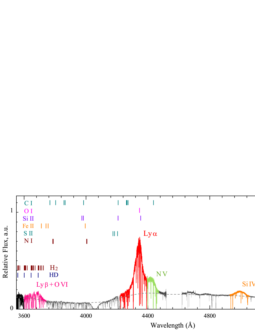
Figure 1: UVES spectrum of Q 1232+082. Emission lines are named and highlighted by different colors, e.g. red for Lyman-$\alpha$, blue for C iv etc. These colors are used in the following figures to indicate where in the spectrum the corresponding measurements are performed. The positions of redshifted absorptions from species discussed in the text are indicated by vertical tick marks. The gray dashed line shows the Q 1232+082 intrinsic continuum derived by fitting regions devoid of emission and absorption lines and interpolating the fit below emission lines. This is the continuum we adopted in the analysis. Note that the spectrum is not flux calibrated.

3 Partial coverage

Partial coverage means that only part of the background source is covered by the absorbing cloud. Mainly this can be the results of (i) the absorbing cloud is smaller than the full projected extent of the background source; (ii) the absorber, although larger than the background source, is porous, e.g. the filling factor of the cloud is not unity. This is readily detectable in the spectrum of the background QSO if a saturated line does not go to the zero level indicating that part of the radiation from the QSO is not shadowed by the cloud. Partial coverage of an emission source by an absorption system is characterised by covering factor which can be defined as the ratio of the flux passing through the absorbing cloud, therefore the flux which is affected by absorption, $F_{\rm cloud}$, to the total flux, $F_{\rm total}$, which is the continuum flux in the spectrum extrapolated over absorption lines;

$$f=\frac{F_{\rm cloud}}{F_{\rm total}},$$ (1)

and the measured flux in the spectrum, $F(\lambda)$, is

$$F(\lambda)=(F_{\rm total}-F_{\rm cloud})+F_{\rm cloud}(\lambda)e^{-\tau(\lambda)},$$ (2)

where $\tau(\lambda)$ is the optical depth of the cloud (see Ganguly et al. 1999). These definitions are illustrated in Fig. 2. The determination of the covering factor is trivial in the case of a highly saturated absorption line (see Fig. 2 cases a) and b)). In case of a partially saturated line (see Fig. 2, c)) several transitions (with possibly different covering factors) must be used.

Absorption lines associated with an absorption system usually span a wide range of wavelengths (see Fig. 1). Therefore we can investigate the dependence of the partial coverage on the position of the lines in the spectrum. Different species are predominantly found in different regions of the cloud, corresponding to different physical properties of the gas (molecular, neutral, ionized) and have absorption lines located on top of different parts of the quasar spectrum attributed to different regions of the AGN (accretion disk, BLR, NLR). We therefore can try to infer information on the spatial extent of both the cloud and the AGN.

In the following, we make a detailed analysis of the $z_{\rm abs}=2.33771$ molecular hydrogen absorption system in the spectrum of Q 1232+082   in order to measure the covering factors of different species relative to different regions of the AGN. We will call Line Flux Residual (LFR) the fraction of the normalized QSO flux which is not covered by the cloud ${\rm LFR}=(F_{total}-F_{cloud})/F_{total}=1-f$ (see Fig. 2). In the following LFR is expressed in percents.

Figure 2: Illustration of the effect of partial coverage on absorption line profiles in three cases: a) a highly saturated line with total coverage, $f=1$; b) a highly saturated line with partial coverage, $f=0.8$; c) a partially saturated line with partial coverage, $f=0.8$ (see Eq. 2). Line Flux Residual (LFR) is the fraction of the QSO flux which is not covered by the cloud and can be easily derived in case b).

3.1 Zero flux level correction

One possible source of uncertainty in the measurement of partial coverage is that the zero flux level of the spectrum is in error due to approximate background or sky subtraction. We have estimated this uncertainty by measuring the flux residual at the bottom of saturated lines located mainly in the Lyman-$\alpha$ forest. Fig. 3 shows the result of this analysis as the percentage of the residual flux relative to the flux in the spectrum versus wavelength. We also show the three lines with the largest error (3.6, 2.9 and 2%). Note that a blend of several non-saturated lines could mimic a saturated (broad) line that does not go to the zero flux level. To avoid as much as possible such lines, we excluded from the analysis the lines for which the width of the wings (shown as the blue regions in the individual panels of Fig. 3) is larger than the full width at half maximum of the line.

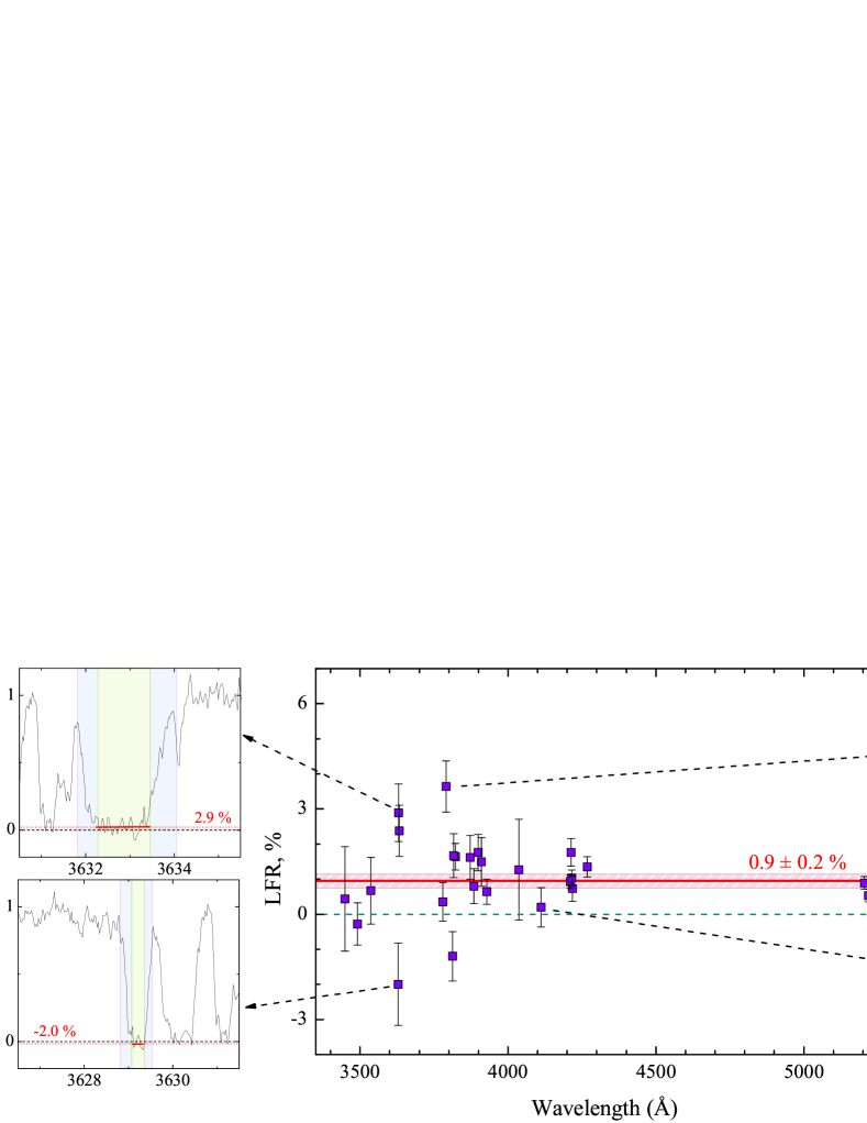
Figure 3: Correction of the zero flux level in the spectrum of Q 1232+082. The line flux residual (LFR) measured in the core of saturated lines (some of them are shown in individual panels, with green and blue regions indicating the core and wings of the lines (see text)) that are not associated with the molecular cloud at $z=2.33771$ is plotted versus wavelength as filled squares. The red horizontal line shows the mean zero level for these lines. Error bars indicate the scatter in the LFR measured in individual pixels.

We did not find any systematic dependence of the effective zero intensity level on wavelength. The average value is found to be $0.9\pm 0.2$% (see Fig. 2) and we correct the spectrum for this. Note that the average flux level measured in the core of the DLA absorption line is found to be $1.8\pm 0.1$% before correction.

3.2 Partial coverage of H₂ absorption lines

Because of the presence of prominent lorentzian wings in J = 0 and 1 H₂ transitions, the H₂ column density in these levels can be accurately measured to be $\log N=$ $19.45\pm 0.10$ and $19.29\pm 0.15$, respectively (Ivanchik et al. 2010). These column densities imply that the optical depth in the center of absorption lines is $\gg 1$, i.e. all absorption lines from the J = 0 and 1 levels are highly saturated. In addition the widths of J = 0 and 1 lines are larger than the instrumental broadening, therefore all J = 0 and 1 absorption lines should reach zero flux level in their center. Nonetheless, it can be seen in the right panel of Fig. 4 that the profiles of these strongly saturated H₂ absorption lines do not go to the zero flux level while the nearby saturated Lyman-$\alpha$ lines do (with an uncertainty $<2$ %, see Sect. 3.1). The residual flux in the H₂ absorption lines reaches $\sim$10 % of the QSO flux at the corresponding positions.

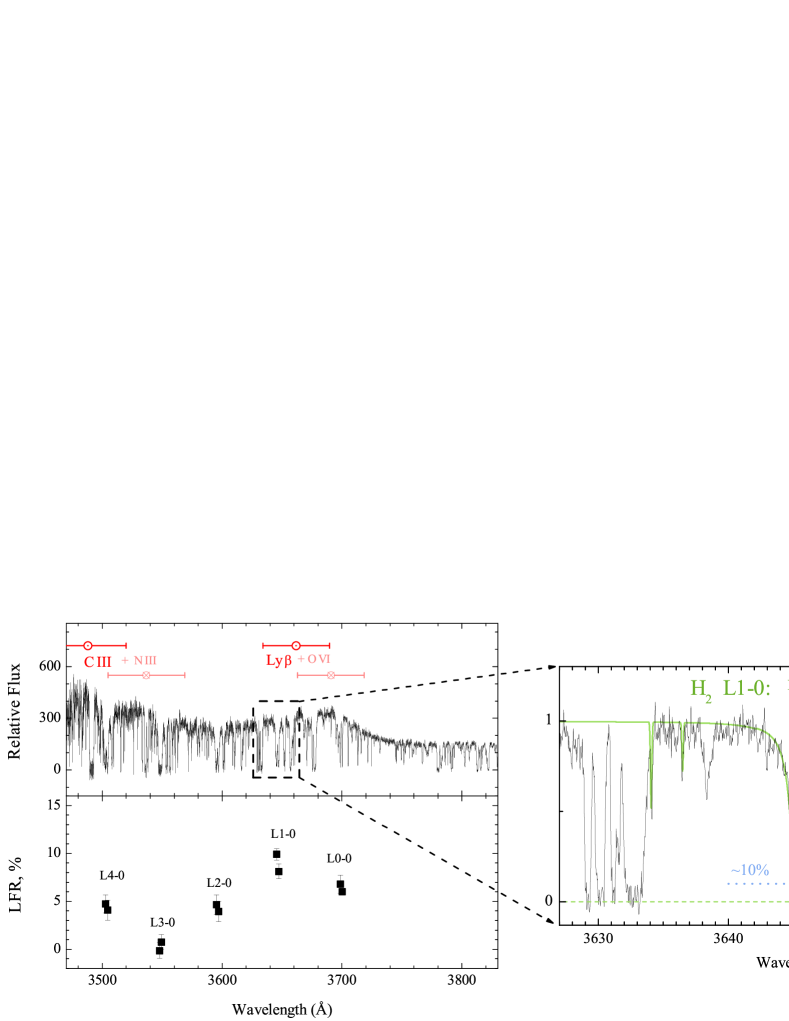
Figure 4: Left top panel: Part of Q 1232+082   spectrum where H₂ absorption lines at $z=2.3377$ are located. Red circles and crosses show the positions of QSO emission lines with error bars indicating line widths taken from Vanden Berk et al. (2001). Right panel: Part of Q 1232+082   spectrum showing absorption lines of the L1-0 H₂ band at $z_{\rm abs}$ = 2.33771. The highly saturated and even damped H₂ lines do not reach the zero flux level whereas several saturated intervening H i Lyman-$\alpha$ absorption lines do. Since these lines are redshifted on top of the Ly$\beta$+O vi emission line from the QSO, this indicates that the H₂-rich molecular cloud covers only part of the Broad Line Region. Left bottom panel: Line flux residuals (LFR) of H₂ absorption lines Error bars indicate the scatter in the LFR measured in individual pixels.

The large number of the H₂ absorption lines and the fact that they are located in the same portion of the spectrum, provides a good opportunity to investigate more the covering factor of the H₂-bearing cloud. Only H₂ absorption lines from the J = 0 and 1 rotational levels are strongly saturated and used to measure the covering factor. We measure the LFR as the average of the flux residuals in the pixels of the bottom of the saturated lines. The corresponding values are shown as filled squares in the left-bottom panel of Fig. 4.

There is a hint for the LFR values to be larger on top of emission lines. This supports the idea that the H₂-bearing cloud covers the central source of continuum but does not cover the whole BLR. The position of these lines are roughly indicated as horizontal segments in Figure 4. Positions and widths of the QSO emission lines are taken from Vanden Berk et al. (2001). Note that Lyman-$\beta$ is blended with O vi and C iii with N iii. Corresponding emissions are clearly seen in the Q 1232+082   spectrum (see upper left panel in Fig. 4). Note that H₂ L3-0 is blended with intervening Lyman-$\alpha$ lines.

3.3 Partial coverage of C i absorption lines

Neutral Carbon absorption lines from the three fine structure levels of the ground state are seen in one single component associated with the H₂ molecular system. These levels are denoted in the following as C i (ground state), C i^∗ (23.6 K above the ground state), and C i^∗∗ (62.4 K above the ground state). The lines from these levels are not highly saturated, span a wide wavelength range in the QSO spectrum $\approx$3800$-$5600 Å  (see Fig. 1) and a wide range of oscillator strengths. In addition, by chance, some of these lines are located on top of the QSO C iv emission line. C i and H₂ are believed to be nearly co-spatial in diffuse molecular clouds (Srianand et al. 2005) and therefore we can expect the C i lines to show partial coverage as well. To estimate the LFR of these lines, we use two different methods, curve-of-growth and profile fitting.

3.3.1 Curve of growth

Atomic data for C i transitions were taken from the Wiese, Fuhr & Deters (1996). Only lines without any apparent blend with absorptions from other species were used in the analysis. The spectrum was normalized with a continuum constructed by fitting spline functions to points devoid of any absorption.

Some of the lines partly overlap with each others because of close wavelengths. If the overlapping lines belong to different C i fine-structure levels (e.g. $\lambda_{0}\approx 1277.2$ Å), then the equivalent width (EW) was measured by fitting simple absorption components with fixed relative velocity shifts (but different central optical depth). If the overlapping lines belong to the same fine-structure level (as for $\lambda_{0}\approx 1329.1$ Å), then we fitted a profile where all the parameters were fixed except one for the central optical depths.

We construct the observed curve-of-growth for C i absorption lines detected in the spectrum (see left panel of Fig. 5). In this figure, black points are for absorption lines located on top of the QSO intrinsic continuum whereas other color points are for absorption lines located on top of an emission line with the color code as indicated on Fig. 1. The best theoretical fit to the black points yields $b=1.85$ km/s. It can be seen in the left panel of Fig. 5 that not only this fit is very good but that most of the other points do not lie on the theoretical curve. These lines have a too small equivalent width.

The large discrepancy between the observed equivalent width and the one expected from the theoretical curve fitted on the lines located on top of the intrinsic quasar continuum is maximum for the blue subset of lines that are located on top of the C iv emission line. It cannot be explained by continuum misplacement since the signal to noise ratio in this part of the spectrum is quite large ($\sim$50). Blending with other absorption lines also cannot explain this discrepancy because blends tend to increase the equivalent widths while we see systematically smaller equivalent widths. On the other hand partial coverage is a reasonable explanation for this discrepancy because it means that part of the background radiation is not intercepted by the absorption system yielding a decrease of the measured equivalent width, $W_{\rm obs}=W(N,b)\cdot f$, where $N$ and $b$ are, respectively, the column density and the Doppler parameter, and $f$ is a covering factor.

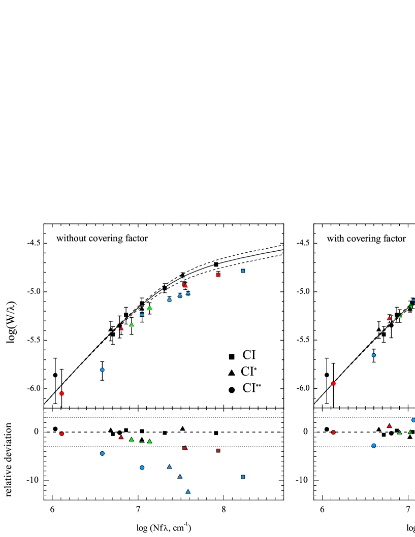
Figure 5: Comparison of the curves-of-growth obtained in two cases: Left hand-side panel: using only absorption lines located on top of the QSO intrinsic continuum (black points). In that case, absorption lines located on top of emission lines (colored points) significantly deviate from this curve; Right hand-side panel: using all the lines but correcting for partial coverage (see Table 1). The error bars represent 1$\sigma$ error determination of the equivalent widths. The dashed lines show the theoretical curve of growth with a Doppler parameter deviating from 1$\sigma$ interval for estimated b-parameter for the best curve-of-growth. Bottom panels show relative deviations of measured equivalent widths from the best curve of growth. Relative deviation of a point is the deviation measured in units of obtained errors for this point. The dotted curves show relative deviations equal to $\pm 3$.

We re-fitted the curve of growth with additional minimization parameters corresponding to the LFR values. Since the C i lines are grouped around similar wavelengths, we applied the same value of LFR for lines that are members of a group. Therefore different LFR values are used for the groups located on top of the C iv, Lyman-$\alpha$ and N v emission lines, respectively (see Fig. 1). The lines located on top of the QSO intrinsic continuum are assumed to fully cover the background source. Our best fit using the new $\chi^{2}$ procedure is presented in the right panel of Fig. 5 and the best fitted parameters are given in Table 1. The derived LFR values are of the order of 20-30 %. The LFR error is found to be larger for the lines located on top of the N v emission line because of larger errors in the continuum placement in this region. The reduced $\chi^{2}$-value after correction for partial coverage is $\approx$1.2 instead of $\approx$3.8 for the case without correction. The $b$ values and C i column densities for the final fit and the fit of the absorption lines that are located on top of the continuum are in agreement which indicates that this partial coverage explanation is quite satisfactory.

3.3.2 Voigt-profile Fitting

We performed Voigt-profile fitting of C i absorption lines to confirm the results obtained from the curve-of-growth analysis. As before, the continuum was locally approximated by spline functions. We fitted the absorption lines adding to usual parameters ($b$ and $N$) a covering factor parameter for each of the three main emission lines of the QSO spectrum (C iv, Lyman-$\alpha$ and N v) to be constrained during the minimization. A few line profiles together with the corresponding fitted spectrum are shown in Fig. 6. In each panel we indicate the required LFR, $\sim$20, 19 and 27 %, respectively, for Lyman-$\alpha$, N v and C iv (see Table 1).

The final reduced $\chi^{2}$ is $\approx$3 when it is $\approx$10 without any correction of partial coverage. Fig. 7 demonstrates that partial coverage correction is indeed needed. Partial coverage makes a line with column density $N$ and therefore optical depth $\tau_{\rm 0}$ look like a line with $\tau_{\rm obs}$ $<$ $\tau_{\rm 0}$. When fitting with the same $N_{\rm o}$ a series of absorption lines, some of which are affected by partial coverage (when on the top of emission lines) and some of which are not affected by partial coverage (when on the top of the intrinsic continuum), the value of $N$ derived from the fit will be smaller than $N_{\rm o}$. Therefore, the fit of the lines affected by partial coverage will be deeper than the absorption line whilst the fit of the lines that are not affected by partial coverage will not be deep enough. This is indeed the case for the $\lambda$1560.682 (not affected) $\lambda$1656.982 Å  (affected) features as can be seen on Fig. 7.

Note that a covering factor parameter was introduced as well for absorption lines located on top of the QSO intrinsic continuum and the best fit is obtained with total coverage of these lines.

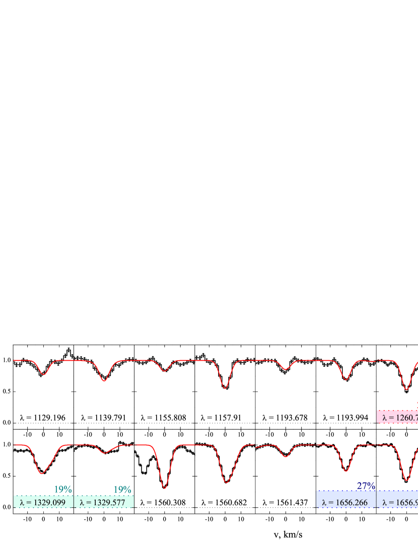
Figure 6: Final Voigt-profile fit of the C i absorption lines. The overall fit is overplotted as a red solid line. Partial coverage of the emission lines (indicated in each panel) is derived from the fit and is found to be $\sim$20 % for Lyman-$\alpha$, 19 % for N v and 27 % for C iv (see Table 1). Colors correspond to the location of the lines in the spectrum as shown in Fig. 1.

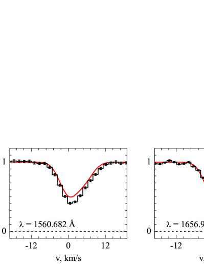
Figure 7: Examples of poorly fitted lines when the fit to all C i transitions is performed without taking into account partial coverage. Left panel shows the case of a line which is not affected by partial coverage. In that case, the fit underestimates the profile because the overall fitted column density is found too small due to the weight of lines affected by partial coverage. Right panel shows the case of a transition affected by partial coverage. In that case the fit overestimates the absorption because the partial coverage decreases the observed optical depth of the transition. Note that the effect is large in the present case because LFR is found to be as large as 27 % for the lines on top of the C iv emission line (see Fig 6).

Results of profile fitting are shown in Table 1. Parameters obtained from curve-of-growth analysis and profile fitting are in excellent agreement with each other and both slightly different from results obtained previously without consideration of partial coverage by Srianand et al. (2005).

value	Curve of growth	Profile fitting	Srianand et al. 2005
$b$ (km/s)	1.85 $\pm$ 0.09	1.84 $\pm$ 0.15	1.70 $\pm$ 0.10
log $N$(C i)	13.87 $\pm$ 0.05	13.87 $\pm$ 0.05	13.86 $\pm$ 0.22
log $N$(C i∗)	13.58 $\pm$ 0.04	13.56 $\pm$ 0.04	13.43 $\pm$ 0.07
log $N$(C i∗∗)	12.83 $\pm$ 0.05	12.82 $\pm$ 0.07	12.63 $\pm$ 0.22
LFR: C iv	29.2 $\pm$ 3.2 %	26.9 $\pm$ 4.4 %
LFR: Ly$\alpha$	20.9 $\pm$ 4.8 %	19.6 $\pm$ 5.3 %
LFR: Ly$\alpha$ + N v	19.1 $\pm$ 6.7 %	19.4 $\pm$ 8.8 %

Table 1: Column densities and Doppler parameters obtained from curve-of-growth analysis and Voigt profile fitting, compared to the results without considering partial coverage (Srianand et al. 2005). Column densities are in units of cm^-2.

3.4 Si ii and O i

In addition to the C i and H₂ transitions studied above, we found two additional absorption lines associated with the $z_{\rm abs}=2.3377$ absorption system and located on top of the QSO Lyman-$\alpha$ emission line that show also partial coverage: $\lambda=1302.2$ Å of O i and $\lambda=1304.4$ Å of Si ii (see Fig. 8). The main component of the O i $\lambda$1302 transition at $v\sim 0$ km/s, has an apparent flat bottom but with non-zero flux at the center of line. This feature cannot be the result of finite spectral resolution as its width is about 50 km/s, much larger than our resolution, FWHM $\sim 6$ km/s. Also the shape is very unlikely to be a combination of many unsaturated lines because all the components, the structure of which can be guessed from Si ii, would have to have exactly the same optical depth. Thus, assuming that there is no error in the zero flux level as ascertained by two saturated lines on both side of the Lyman-$\alpha$ emission line, the LFR for this line is $\sim$6 %.

We detect six Si ii transitions at $z=2.3377$. One of them (Si ii $\lambda$1304) is located on top of the Lyman-$\alpha$ emission line as well and is expected to show partial coverage as O i $\lambda$1302. The others are located on top of the continuum only. We performed a joint fit of the Si ii and O i lines, using seven components (one of them found coincident with the molecular component at $z=2.33771$) and allowing for partial coverage for O i$\lambda$1302 and Si ii$\lambda$1304. We have tied up together the velocity positions of the seven components and let the other parameters vary (Doppler widths and column densities). We find the values of LFR for these lines are 6.2 % and 7.5 % for O i and Si ii$\lambda$1304 respectively. We have minimized the number of free parameters using one LFR value for all components of each absorption profile: O i$\lambda$1302 Å  and Si ii$\lambda$1304 Å. The O i component at $-80$ km/s could have LFR slightly larger than the main component at $v=0$ km/s. However, the width of the component is only $\sim$20 km/s and the bottom of the line is not perfectly flat. Therefore, we have no strong argument to claim that LFR is larger for this component.

We have fitted the Si ii and O i absorption features together with the corresponding Al ii$\lambda$1670 and C ii$\lambda$1334 transitions. The results of the fit is presented in the left-hand side panel of Fig. 8. where LFR for Si ii$\lambda$1304 and O i$\lambda$1302 are illustrated by red stripes. Note that the possibility is left to have a LFR of $\approx$2 % for each of the Al ii$\lambda$1670 and C ii$\lambda$1334 transitions which are located in the far wings of the N v and C iv emission lines, respectively. We find however that this value is too close to the average error in the zero flux level to be confident it is real.

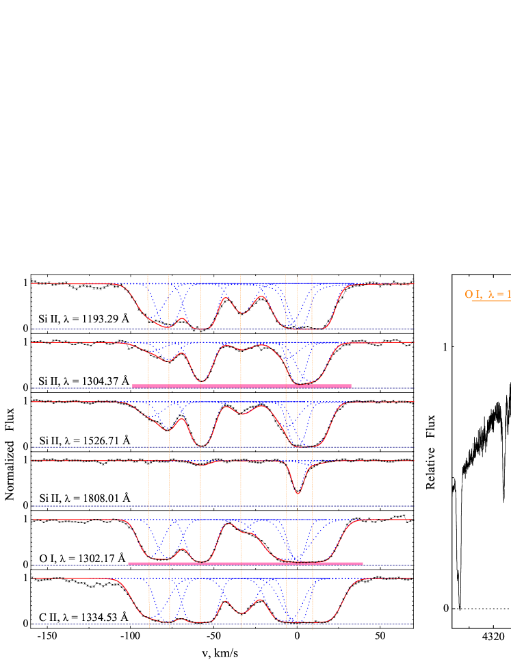
Figure 8: Si ii, O i and C ii absorption features at $z=2.3377$ in the Q 1232+082   spectrum. Results from Voigt profile fitting together with components are overplotted in the left hand side panel. The velocity origin is taken at the position of the H₂-bearing component. The right panel shows the location of the O i  $\lambda$1302 and Si ii$\,\,\lambda$1304 absorption lines on top of the QSO Lyman-$\alpha$ emission line together with two saturated lines going to the zero level on both sides.

3.5 Other species

Numerous other absorption lines from Fe ii, S ii and N i are present in the spectrum. N i transitions are located in a wavelength range devoid of QSO emission lines while some lines of Fe ii and S ii fall partially in the wings of emission lines (see Fig. 1). These absorption lines are not highly saturated and have similar line strengths, which makes the determination of the covering factor unreliable. For example, the three S ii lines are located in the wing of the QSO Lyman-$\alpha$ emission line. The profile fitting analysis of the three lines indicates that a LFR of 11$\pm$5% is slightly preferred to full coverage (see Fig. 9). A standard statistical analysis yields a reduced $\chi^{2}$ of 2.8 when partial coverage is allowed instead of 3.7 with full coverage. We think however that the conclusion of partial coverage for the S ii lines is only tentative.

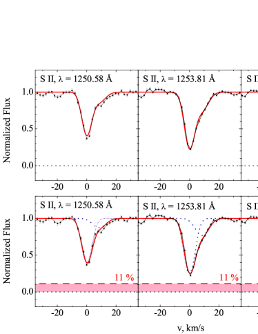
Figure 9: S ii absorption lines associated with the $z=2.3377$ absorption system. The results of two variants of a two component fit are presented. The top panels are for full coverage and the lower panels for a LFR of 11%.

3.6 Overview

We have shown above that the neutral part of the absorbing cloud covers the source of the intrinsic quasar continuum completely but only partly the broad emission line region. We therefore are interested in which fraction of the BLR is covered by the cloud.

For this, we estimate the fraction of the total flux emitted by the continuum source at the location of the emission lines. This is done using the spectral shape of the intrinsic continuum as shown in Fig. 1. It is obtained by extrapolating the continuum below the emission lines by splines functions fitted in the regions devoid of any emission or absorption lines. We thus can estimate both the fluxes from the BLR, F_BLR, and the continuum. Using the values of LFR derived in the previous Sections and the fact that the cloud covers the continuum completely, it is straightforward to derive the covering factor of the BLR for different emission lines $\rm f=1-(LFR\cdot F_{total})/F_{BLR}$. Results are summarized in Table 2.

When estimating the errors, we have taken into account the errors on LFR but also a $\sim$20-30% uncertainty on the QSO intrinsic continuum placement below the emission lines. Note that for further discussion we use only covering factors of C iv and Lyman-$\alpha$ emission lines.

	O vi	Lyman-$\alpha$	N v	C IV
H2	$0.80^{+0.07}_{-0.11}$
C i		$0.38^{+0.16}_{-0.32}$	$0.56^{+0.14}_{-0.21}$	$0.47^{+0.07}_{-0.12}$
O i		$0.93^{+0.02}_{-0.02}$
Si ii		$0.91^{+0.02}_{-0.03}$

Table 2: Covering factors of different emission line regions (columns) by different species (rows) after taking into account the fact that the QSO intrinsic continuum is fully covered. We note that the most reliable measurement is for C iv emission line (see text).

4 Physical conditions in the DLA system

If we could estimate the size of the intervening H₂-bearing molecular cloud, we could estimate the size and, possibly, the structure of the QSO BLR using the covering factors derived in the previous Section. Therefore, we will first study the physical conditions in the gas.

4.1 Ionization structure of the $z=2.3377$ absorption cloud

The absorption profiles of different species are shown in Fig. 10 ranked following the ionization potential of the corresponding ion. The H₂-rich component is traced by HD and neutral species Mg i, Fe i, Si i, S i, C i and Cl i. The latter species is closely tied up to H₂ by charge exchange reaction processes. We tentatively detect Fe i and Si i absorptions, associated with the molecular component. The measured column densities $\log(N)$ are 11.86$\pm$0.09 and 12.68$\pm$0.18 for Si i and Fe i, respectively. These ions are detected only in a few QSO absorption systems (D’Odorico 2007; Quast, Reimers & Baade 2008) and indicate the presence of cold and well shielded gas. Neutral sulphur is rarely seen in QSO absorption systems but it is seen in five absorption systems with associated CO detection (Srianand et al. 2008; Noterdaeme et al. 2009; Noterdaeme et al. 2010; Noterdaeme et al. 2011). We therefore carefully searched for CO absorptions in the Q 1232+082   spectrum. Unfortunately, we could place only a 3 $\sigma$ upper limit on CO column density from the non-detection in the three strongest band at 1447 Å, 1477 Å  and 1509 Å: log $N$(CO) $<$ 12.6. The singly and twice ionized species span about 150 km s^-1 bluewards of the H₂-bearing molecular component.

The ionization structure indicates that a large fraction of the metals could be associated with the molecular component. This is the case of low ionization species (E$<13.6$ eV) but also of higher ionization species (see for example S ii and Si ii absorption profiles). This indicates that the cloud is concentrated around the central H₂-bearing component.

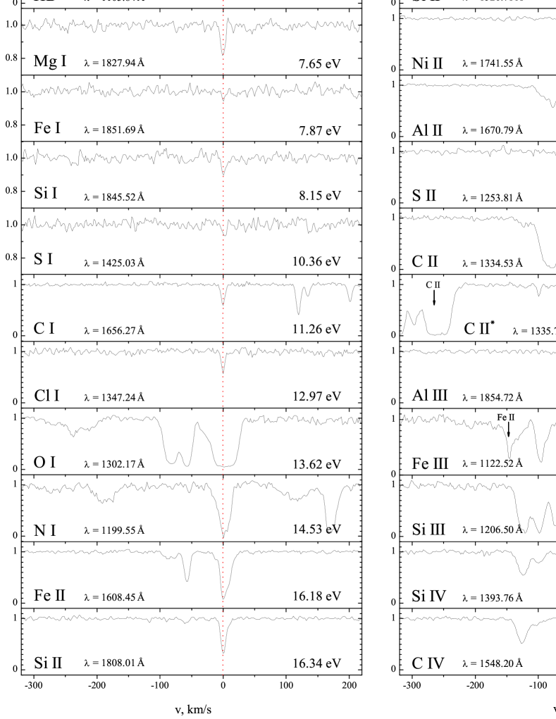
Figure 10: Absorption profiles of different species in the $z=2.3377$ DLA system towards Q 1232+082. The origin of the velocity scale is taken at the redshift of the H₂ component, $z=2.33771$.

4.2 Metal content

We have fitted all the absorption lines which are not strongly saturated using Voigt-profiles, derived total column densities and calculated metallicities as [X/H] = log $N$(X)/$N$(H i) $-$ log [$N$(X)/$N$(H i)]_⊙ with solar metallicities taken from Lodders (2003). Results are given in Table 3 and are summarised in Fig. 11. The mean metallicity as indicated by the Sulfur metallicity which has smallest error is [S/H] = $-$1.32$\pm$0.12. It is remarkable that, within errors, [S/H] $\sim$ [Si/H], which indicates little depletion of Si.

Note that [Cl i/H] $\sim$ [S/H] seems at odd. As Cl i is coupled with H₂ via charge exchange reactions (Jura 1974), Cl i comes from the H₂-bearing component. Since we measure a high Cl i column density, this H₂ bearing component must have a large molecular fraction ($>$0.25, see Abgrall et al. 1992).

Therefore, in principle the Cl metallicity could be much higher since we should divide the Cl i column density by 2$\times$$N$(H₂) and not by the total hydrogen column density ($N$(H i)+2$N$(H₂)), as we have done in Table 3. This would give a metallicity close to solar in the H₂ bearing component [Cl i/2H₂]$<$ $-$0.27$\pm$0.17. This is an upper limit as the cloud could be partially molecular only.

It is likely that most of the Si ii is to be found associated with the molecular component (see Fig. 8, $\lambda$=1808 Å line). This further suggests that the cloud is concentrated around the clumpy central component of higher metallicity.

Relative abundance of nitrogen to $\alpha$ elements, i.e. [N/S], [N/Si] is $\sim-1$, that is consistent with typical low nitrogen metallicity in DLAs (Petitjean, Ledoux & Srianand 2008; Pettini et al. 2008). Iron, Nickel and Manganese are observed to be depleted by a factor $\sim$5 relative to Sulfur. This moderate depletion probably onto dust-grains supports the idea that the presence of even little amount of dust favors the formation of molecular hydrogen.

Species	log $N$	[X/H]a
N i	$14.54\pm 0.22$	$-2.23\pm 0.24$
Mg ii	$15.33\pm 0.24$	$-1.16\pm 0.25$
Si ii	$15.06\pm 0.05$	$-1.42\pm 0.09$
P ii	$12.86\pm 0.24$	$-1.54\pm 0.25$
S ii	$14.81\pm 0.09$	$-1.32\pm 0.12$
Cl i	$12.97\pm 0.14$	$-1.23\pm 0.16$
Ar i	$13.86\pm 0.22$	$-1.63\pm 0.24$
Mn ii	$12.22\pm 0.08$	$-2.22\pm 0.11$
Fe ii	$14.44\pm 0.08$	$-1.97\pm 0.11$
Ni ii	$12.81\pm 0.04$	$-2.35\pm 0.09$

Table 3: Column densities (in units of cm^-2) and metallicities relative to solar in the $z=2.33771$ DLA system. ^a  Relative to solar. Solar abundances are taken from Lodders (2003).

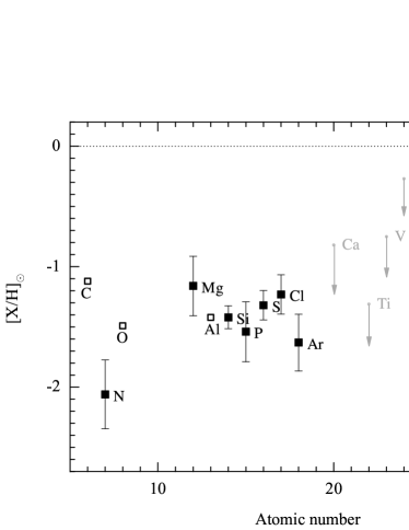
Figure 11: Metallicities relative to solar in the $z=2.33771$ absorption system toward Q 1232+082. Empty squares show C, O and Al metallicities derived from saturated lines and should be considered as lower limits.

4.3 Number densities

4.3.1 C i Fine structure

In Section 3.3 we have measured the column densities of C i atoms in the fine structure levels of the ground state. The balance between the different level populations can be used to estimate the number density in the gas. Radiative pumping of C i excited states is probably not important since to explain the measured column density ratios the UV radiation field should be about 50 times higher than the mean Galactic value (see the discussion in Silva & Viegas (2002) and Noterdaeme et al. (2007)). Such a high UV radiation field is very unlikely for this one component system in which low ionization species dominate. We also assume the CMBR temperature to be $T_{\rm CMBR}$ =2.73 $\times(1+2.3377)$ K, following standard cosmology model. Under these two assumptions, and considering a homogeneous cloud, the relative populations of the C i levels depend only on the number density and the temperature. Collision coefficients were taken from Schröder et al. (1991), assuming that the main collisional partner is H₂. We take for the temperature in the cloud the value, $T_{\rm kin}$ = 67$\pm$11 K, derived from the analysis of the molecular hydrogen ortho-para ratio (Ivanchik et al. 2010). Confidence contours for $n_{\rm H_{2}}$ are shown on Fig. 12. The best value for the density is $n_{\rm H_{2}}$ = 105${}^{+27}_{-24}$ cm^-3 with 1$\sigma$ uncertainty.

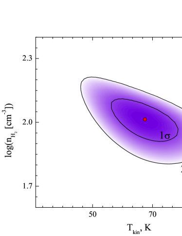
Figure 12: Confidence contours for the physical conditions derived from the relative populations of the C i fine structure levels and the populations of the first two rotational levels of H₂.

4.3.2 HD rotational levels

We can derive an upper limit on the J = 1 HD column density from the most prominent absorption lines shown in Fig. 13. All other HD J = 1 transitions are partly or fully blended. We find log $N$(HD, J=1) $<$ 14.1. The measured $N$(HD, J=1)/$N$(HD, J=0) upper limit is in agreement with what is expected in HD/H₂ molecular clouds (Le Petit, Roueff & Le Bourlot 2002) and can be used to derive an upper limit on the number density in the cloud. For this, we follow the analysis of Balashev, Ivanchik & Varshalovich (2010) who have detected recently HD J = 1 absorptions at $z$ =2.626 towards J 0812+032. Likewise the C i analysis, we can neglect radiative pumping. In spite of excitation energies of HD levels being higher than those of C i (which makes collisions less effective), self-shielding processes become rapidly important for HD. We assume the temperature in the cloud is given by the H₂ excitation temperature, $T_{\rm kin}$ = 67$\pm$11 K and that H₂ is the main collisional partner (with collisional coefficients taken from Flower et al. (2000)). The upper limit on the density is $n_{\rm H_{2}}<$160 cm^-3, in agreement with the value derived from C i.

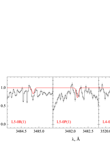
Figure 13: Expected location of HD(J=1) lines from the $z=2.33771$ absorption system toward Q 1232+082.

4.3.3 C ii fine structure

Singly ionized carbon is mostly located in a region surrounding the H₂-rich molecular core of the cloud. Therefore, from the excitation of its fine structure level it is possible to estimate the number density in the envelope of the molecular-rich cloud. From the $\lambda=1335.7$ Å  line (see Fig. 10), we measure log $N$(C ii^∗) = 13.92$\pm$0.15. Unfortunately it is not possible to measure $N$(C ii) directly as the C ii$\lambda$1334 absorption line is strongly saturated (see Fig. 8) and we have to estimate it indirectly (see Srianand, Petitjean & Ledoux 2000). It is known, that the metallicity of the $\alpha$-chain elements is enhanced compared to carbon by a factor of about two, when the mean metallicity is low (i.e. $<-1.0$). Therefore, we consider that $Z$(C) = $Z$(Si)/2 and derive log $N$(C ii) = 15.6$\pm$0.3. In a neutral medium, the upper level of C ii is predominantly excited by collisions with hydrogen (Silva & Viegas 2002; Srianand et al. 2005). This assumption is supported by the velocity structure of O i which traces the neutral gas and is present over the whole C ii absorption profile. The probability of the ground state fine structure transition 3/2 $\to$ 1/2 is $A_{21}\sim 2.29\times 10^{-6}$ s^-1 and the excitation rate with atomic hydrogen is taken from Silva & Viegas (2002). For the range in temperature $T$ $\sim$ 100 $-$ 2000 K, we estimate the density of the neutral region, $n_{\rm HI}$ = 32${}^{+34}_{-21}$ cm^-3. This is smaller but not very different from the density found for the molecular-rich core.

5 Discussion

In this Section we discuss several interpretations to explain partial coverage of QSOs by an intervening cloud: binary quasars, gravitational lensing and transverse dimensions. These explanations are schematically pictured in Fig. 14. In our case and as shown in previous Sections, the continuum source is fully covered by the molecular cloud when the BLR seems to be partially covered by the dense and neutral part of the cloud but also by part of the singly ionized species.

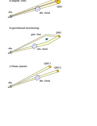
Figure 14: Illustration of the possible explanations for the partial coverage of QSOs by an intervening absorption system.

5.1 Binary quasars

Binary quasars are thought to be the consequence of a galaxy merging event and are observed with separations as small as approximately 10 kpc (Hennawi et al. 2006; Foreman, Volonteri & Dotti 2009; Rodriguez et al. 2006; Vivek et al. 2009). At redshift $z\sim 2$ binary quasars with transverse distance $\lesssim 3\,{\rm kpc}$ would be unresolved by UVES observations. Partial coverage can be seen in case the background source is a binary quasar if the absorbing cloud covers one of the quasars and not the other. However, in such a situation, the intrinsic continuum source would not be covered completely. This is not the case of the z=2.3377 absorption system towards Q 1232+082 which covers the intrinsic continuum completely.

5.2 Gravitational Microlensing

Gravitational lensing (especially microlensing) is one of the explanations for partial coverage. In the simplest case of the quasar being macro-lensed by a galaxy or a galaxy cluster, there is no difference in the QSO image spectra. We therefore expect partial coverage of both the BLR and the intrinsic continuum. Since in the present case, the cloud is very small, the contrary would need a very special configuration.

Observations by Sluse et al. (2007) and Wucknitz et al. (2003) indicate that additional microlensing by stars or objects with mass $\sim 10^{4}M_{\odot}$ can enhance part of the spectrum (continuum and/or a fraction of the BLR) in only one image. If the continuum is strongly enhanced compared to the BLR in the image that is not covered by the cloud, then partial coverage in the continuum could stay unnoticed. However, this explanation would request again a very special situation.

Indeed, if we consider the spectrum as a superposition of a continuum and emission lines, $F=F_{\rm em}+F_{\rm c}$, then in case two images are macrolensed with factors $M_{1}$ and $M_{2}$ and only one image is microlensed with a factor $\mu$, the fluxes in the two images are:

$$F_{1}=M_{1}\cdot F_{\rm em}+M_{1}\cdot F_{\rm c}$$ (3)

$$F_{2}=M_{2}\cdot F_{\rm em}+M_{2}\cdot\mu\cdot F_{\rm c}.$$ (4)

In the simple case of the absorption system being located in front of the microlensed image and totally absorbing it, the measured covering factors in the continuum, ${f}_{\rm c}$, and in the emission line, ${f}_{\rm em}$, will be:

$${f}_{\rm c}=\left(\frac{F_{2}}{F_{1}+F_{2}}\right)_{\rm c}=\frac{M_{2}\cdot\mu}{M_{2}\cdot\mu+M_{1}}$$ (5)

$${f}_{\rm em}=\left(\frac{F_{2}}{F_{1}+F_{2}}\right)_{\rm em}=\frac{M_{2}}{M_{1}+M_{2}},$$ (6)

In the case of the absorber in front of Q 1232+082, we observe $f_{\rm em}\sim 0.5$ and $f_{\rm c}\gtrsim 0.98$ (from zero level correction see Sect. 3.1). This would imply $M_{1}\sim M_{2}$ but more importantly requires a probably unreasonably large microlensing effect $\mu\gtrsim 50$.

5.3 BLR kinematics and size in Q 1232+082

We discuss here the information we can derive on the size of the BLR from the observation and analysis presented above. For this we use over-simplified models considering spherical geometry. This is speculative but given the lack of information on the exact geometrical and kinematical structure of the BLR (Denney et al. 2010), may still be interesting.

The most probable explanation for partial coverage of the Q 1232+082   BLR by the $z=2.3377$ absorption system is that the transverse size of the cloud is smaller than the projected size of the BLR. Following the standard paradigm for Active Galactic Nucleus (AGN), the QSO emission takes place in different regions of different sizes. Therefore, if the transverse extent of the intervening cloud is smaller than the maximum extent of the background source, partial coverage can happen. The inner part of the accretion disk produces the continuum emission. Linear size of the disk is of the order of $l_{\rm disk}<10^{15}\,$cm (Dai et al. 2010 and references within), corresponding to $\theta_{\rm disk}\approx 10^{-6}$ mas at $z=2.57$ (with $h_{100}=0.72$, $\Omega_{M}=0.27$, $\Omega_{\Lambda}=0.73$). The linear size of the BLR is several orders of magnitude larger than the size of the accretion disk and of the order of $\sim 1\,$pc (e.g. Wu et al. 2004; Kaspi et al. 2005). Thus the angular size of the BLR is limited to about $\theta_{\rm BLR}\lesssim 10^{-2}$ mas. In addition, the BLR is supposed to be stratified, the low ionization lines having larger extent than the high-ionization ones (Peterson 1993).

We have estimated the number densities in the cloud: $n_{\rm H2}$ $\sim$ 110 cm^-3 for the H₂-bearing molecular core and $n_{\rm H}$ $\sim$ 30 cm^-3 for the neutral envelope. Given the column density, $N$(H₂) = $4.78\pm 0.96$ $\times$10¹⁹ cm^-2, this gives $l_{\rm H2}$ $\sim$ $0.15^{+0.05}_{-0.05}$ pc for the linear size of the H₂-bearing molecular core along the line of sight. This should also correspond to the size of the C i cloud. Indeed the kinematical structure of the H₂, HD, C i and Cl i absorption features show a single narrow component at the same position (see Fig. 10). Remember also that Cl i and H₂ are tied up (see e.g. Noterdaeme et al. 2010). With the assumption that the transverse size of the cloud is of the same order of magnitude as the longitudinal size, we find that this is small enough to explain the partial coverage of the BLR. To estimate the BLR size we assumed that the cloud and BLR are spherical in shape, and used

$$L_{\rm BLR}=L_{\rm abs}\times K_{\rm cosm}\times K_{\rm geom},$$ (7)

where $L_{\rm BLR}$ and $L_{\rm abs}$ are the transverse sizes of the BLR and the absorber, respectively. $K_{\rm cosm}$ is a cosmological correction factor due to the fact that the QSO and the absorption cloud have different redshifts. In the standard cosmological model and because the redshifts are similar ($z_{\rm em}$ = 2.57 and $z_{\rm abs}$ = 2.3377), this factor is about 1. $K_{\rm geom}$ is a coefficient that depends on the alignment of the two objects and therefore on the distance, $l$, between the two projected centers. Given the dimension of the absorber, we can calculate the most probable dimension of the background source for an observed covering factor. Since the absorber and the background sources are not related, the alignment is random and the probability that $l=l_{0}$ is proportional to $l_{0}$. Therefore, one can calculate the probability distribution function for $K_{\rm geom}$ and obtain the best value of $K_{\rm geom}$ and its errors. Using the measured covering factor, $\sim$0.47, for the C iv emission line, we derived this way a size of the C iv BLR $R_{\mbox{C\,{\sc iv}}}$ $\sim$ $0.18^{+0.08}_{-0.11}$ pc. A schematic representation of this situation is illustrated on Fig. 15.

We can use the size$-$luminosity relationship derived from reverberation mapping (Peterson et al. 2005, Kaspi et al. 2007) to estimate the size of the C iv BLR to be compared with our results. We estimate the luminosity of Q 1232+082, $\lambda$$L_{\lambda}$(1350 Å) (erg/s), to be $\sim$10^46.9. Using Fig. 6 of Kaspi et al. (2007) we derive a C iv lag of the order of 300 days, corresponding to about 0.26 pc. Note that recently, the study of differential microlensing in Q 2237+0305 (Sluse et al. 2010) yielded similar results for the size of the C iv BLR, $0.06^{+0.09}_{-0.04}$ pc. The same typical size is obtained from the study of GeV break in blazars (Poutanen & Stern 2010).

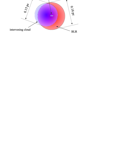
Figure 15: Partial coverage of Q 1232+082   BLR by an intervening absorption cloud at $z=2.3377$. Geometry is assumed spherical. The estimated size of the BLR corresponds to the C iv emission line region covered at 48%.

On the other hand, for the neutral phase, we have $N$(H i) = 7.94$\times$10²⁰ cm^-2 and therefore $l_{\rm HI}$ $\sim$ $8.2^{+6.5}_{-4.1}$ pc. Remember that the neutral phase of the cloud as traced by O i and Si ii covers only $\sim$94% of the Lyman-$\alpha$ emission. The large size we derive for the neutral cloud extent seems in contradiction with the above small size of the C iv BLR. However, it must be reminded that the O i and Si ii are located nearly exactly on top of the Lyman-$\alpha$ emission line. This would mean that the Lyman-$\alpha$ BLR is probably fully covered but that the Lyman-$\alpha$ emission extends well beyond the extent of the C IV emitting BLR. In turn this means that the extended Lyman-$\alpha$ emission corresponds to about 6 % of the flux at the peak of the emission. Note that the velocity difference between O i  $\lambda$1302 and Si ii  $\lambda$1304 is $\sim$500 km/s. Therefore, as can be seen on Fig. 8, right panel, the kinematics of the region which is not covered must be of this order. Unfortunately, we cannot go farther in our derivation of the extent of the Lyman-$\alpha$ emission.

The determination of the BLR size $R_{\rm BLR}$ allows us to estimate the mass of the central black-hole, associated with Q 1232+082   assuming that the BLR is virialized:

$$M_{\rm BH}=\phi\frac{R_{\rm BLR}\Delta V^{2}}{G},$$ (8)

where $\phi\approx 5.5$ is a scale factor (Peterson et al. 2004) and $G$ is the gravitational constant. We estimate the width of the C IV emission line $\Delta V=2463^{+12}_{-24}$ km/s, which is less than the value $\sigma_{v}\approx 2780$ km/s derived by Vanden Berk et al. (2001). We find $M_{\rm BH}$ = 6.8${}^{+4.1}_{-4.5}$$\times$10⁸ M_⊙. This is slightly lower than the mean BH mass derived by Vestergaard et al. (2008) for quasars of this luminosity at this redshift but well within the overall scatter.

6 Conclusion

The analysis of H₂, C i, O i and Si ii absorption lines from the molecular DLA system at $z_{\rm abs}$ = 2.3377 toward Q 1232+082  has shown that the intervening absorbing cloud is not covering the background source totally. We used a curve-of-growth and a profile fitting analysis to estimate the partial covering factor. The different methods yield covering factors of the H₂-bearing core (as traced by H₂ and C i) to be $\approx$ 48, 66 and 75 % for the C iv, C iii and Lyman-$\beta$-O vi emission lines whilst the QSO intrinsic continuum is covered completely. The O i $\lambda$1302 and Si ii $\lambda$1304 absorptions cover only $\sim$94% of the Lyman-$\alpha$ emission.

According to the generally accepted model of AGNs, broad emission lines are emitted by warm and highly ionized gas located in the BLR with transverse dimension of the order of $\sim$1 pc. The quasar continuum is produced by the inner part of the accretion disk, which linear size is several orders of magnitude less than the BLR size. Thus the most probable explanation of the observed partial coverage is the comparable angular sizes of the BLR and the compact H₂-bearing absorption cloud. The fact that the continuum is completely absorbed makes other explanations such as the presence of a binary quasar or gravitational lensing less plausible.

We derived the linear extent of the H₂-bearing cloud and neutral envelope to be $l_{\rm H_{2}}$ $\sim$ $0.15^{+0.05}_{-0.05}$ pc and $l_{\rm HI}$ $\sim$ $8.2^{+6.5}_{-4.1}$ pc, respectively. Assuming that the H₂-bearing component is spherical in shape, we estimate the size of the C iv BLR to be $\sim$0.2 pc. The large size we derive for the neutral cloud extent together with the covering factor of $\sim$94% of the Lyman-$\alpha$ emission means that the Lyman-$\alpha$ BLR is probably fully covered but that the Lyman-$\alpha$ emission extends well beyond the extent of the C IV emitting BLR. In turn this means that the extended Lyman-$\alpha$ emission corresponds to about 6 % of the flux at the peak of the emission (over $\sim$500 km/s). Assuming the C iv BLR is virialized, we derive the mass of the central $M_{\rm BH}$ = 6.8${}^{+4.1}_{-4.5}$$\times$10⁸ M_⊙

Partial coverage of the background source by intervening clouds has been observed an used to derive the radius of the clouds when the background source is the combination of several gravitational images (Petitjean et al., 2000a; Ellison et al., 2004). This is the first time that partial coverage of a QSO BLR by an intervening cloud is reported.

This kind of situation tests the kinematics of the BLR. Indeed we see that the covering factor depends of the position of the absorption on top of the emission line. This can be due to the presence of inflows or outflows in BLR (Denney et al. 2009) which could be covered differently or the BLR could have a disk-like structure implying the projected velocity is correlated with the spatial position. Obviously it will be difficult to disentangle the different kinematics. However, it may be interesting to dramatically increase the quality of spectra in which an intervening compact absorption system is observed. This may reveal that partial covering factor is not unusual and could be used to constrain the BLR structure.

Acknowledgments. This work was supported in part by a bilateral program of the Direction des Relations Internationales of CNRS in France, by the Russian Foundation for Basic Research (grant 11-02-01018a), and by a State Program “Leading Scientific Schools of Russian Federation” (grant NSh-3769.2010.2), by Ministry of Education and Science of Russian Federation (contract # 11.G34.31.0001 with SPbSPU and leading scientist G.G. Pavlov). PPJ and RS acknowledge support from the Indo-French Centre for the Promotion of Advanced Research under the programme No.4304–2. SB thanks Dynasty Foundation and A.M. Krassilchtchikov for help with cluster computations.

References

- Abgrall et al. (1992) Abgrall H., Le Bourlot J., Pineau des Forêts G., Roueff E., Flower D. R., Heck L., 1992, A&A, 253, 525
- Balashev et al. (2010) Balashev S. A., Ivanchik A.V., Varshlovich D. A., 2010, Astron. letters, 36, 761
- Bentz et al. (2009) Bentz M. C., Peterson B. M., Netzer H., Pogge R. W., Vestergaard M., 2009, ApJ, 697, 160
- Blandford & McKee (1982) Blandford R. D., McKee C. F., 1982, ApJ, 255, 419
- Dai (2010) Dai X., Kochanek C. S., Chartas G., Kozlowski S., Morgan C. W., Garmire G., Agol, E., 2010, ApJ, 709, 278
- D’Odorico (2007) D’Odorico V., 2007, A&A, 470, 523
- Denney et al. (2010) Denney K. D. et al., 2010, ApJ, 721, 715
- Denney et al. (2009) Denney K. D. et al., 2009, ApJ, 704, 80
- Ellison et al. (2004) Ellison S. L., Ibata R., Pettini M., Lewis G. F., Aracil B., Petitjean P., Srianand R., 2004, A&A, 414, 79
- Ellison et al. (1999) Ellison S. L., Lewis G. F., Pettini M., Sargent W. L. W., Chaffee F. H., Foltz C. B., Rauch M., Irwin M. J., 1999, PASP, 111, 946
- Flower et al. (2000) Flower D. R., Le Bourlot J., Pineau des Forets G., Roueff E., 2000, MNRAS, 314, 753
- Foreman et al. (2009) Foreman G., Volonteri M., Dotti M., 2009, ApJ, 693, 1554
- Ganguly et al. (1999) Ganguly R., Eracleous M., Charlton J. C., Churchill C. W. 1999, AJ, 117, 2594
- Ge & Bechtold (1999) Ge J., Bechtold J., 1999, in Carilli C. L., Radford S. J. E., Menten K. M., Langston G. I., eds, ASP Conf. Series Vol. 156, Highly Redshifted Radio Lines, p. 121
- Hamann (1997) Hamann F., 1997, ApJS, 109, 279
- Hennawi et al. (2006) Hennawi J.F. et al., 2006, AJ, 131, 1
- Jura (1974) Jura M., 1974, ApJ, 190, L33
- Ivanchik et al. (2010) Ivanchik A.V., Petitjean P., Balashev S.A., Srianand R., Varshalovich D. A., Ledoux C., Noterdaeme P., 2010, MNRAS, 404, 1583
- Kaspi et al. (2005) Kaspi S., Maoz D., Netzer H. Peterson B. M., Vestergaard M., Jannuzi B. T., 2005, ApJ, 629, 61
- Kaspi et al. (2007) Kaspi, S., Brandt, W. N., Maoz, D., Netzer, H., Schneider, D. P., & Shemmer, O. 2007, ApJ, 659, 997
- Ledoux et al. (1998) Ledoux C., Théodore B., Petitjean P., Bremer M. N., Lewis G. F., Ibata R. A., Irwin M. J., Totten E., 1998, A&A, 339, L77
- Ledoux et al. (2003) Ledoux C., Petitjean P., Srianand R., 2003, MNRAS, 346, 209
- Le Petit et al. (2002) Le Petit F., Roueff E., Le Bourlot, J., 2002, A&A, 390, 369
- Lewis et al. (2002) Lewis G. F., Ibata R. A., Ellison S. L., Aracil B., Petitjean P., Pettini M., Srianand R., 2002, MNRAS, 334, L7
- Lodders (2003) Lodders K., 2003, ApJ, 591, 1220
- Netzer (1997) Netzer H., Peterson B. M., 1997, ASSL, 218, 85
- Noterdaeme et al. (2007) Noterdaeme P., Ledoux C., Petitjean P., Srianand R. 2007, A&A, 469, 425
- Noterdaeme et al. (2008) Noterdaeme P., Ledoux C., Petitjean P., Srianand R. 2008, A&A, 481, 327
- Noterdaeme et al. (2009) Noterdaeme P., Ledoux C., Srianand R., Petitjean P., Lopez S., 2009, A&A, 503, 765
- Noterdaeme et al. (2010) Noterdaeme P., Petitjean P., Ledoux C., López S., Srianand R. and Vergani S. D. 2010, A&A, 523, 80
- Noterdaeme et al. (2011) Noterdaeme P., Petitjean P., Srianand R., Ledoux C., López S. 2011, A&A, 526, L7
- Peterson (1993) Peterson B. M., 1993, PASP, 105, 247
- Peterson & Wandel (1999) Peterson B. M., Wandel A., 1999, ApJ, 521, L95
- Peterson et al. (2004) Peterson B. M., et al., 2004, ApJ, 613, 682
- Petitjean et al. (1994) Petitjean P., Rauch M., Carswell R. F., 1994, A&A, 291, 29
- Petitjean et al. (2000a) Petitjean, P., Aracil, B., Srianand R., Ibata R., 2000a, A&A, 359, 457
- Petitjean et al. (2000b) Petitjean P., Srianand R., Ledoux C. 2000b, A&A, 364, L26
- Petitjean et al. (2008) Petitjean P., Ledoux C., Srianand R. 2008, A&A, 480, 349
- Pettini et al. (2008) Pettini M., Zych B. J., Steidel C. C., Chaffee F. H., 2008, MNRAS, 385, 2011
- Poutanen et al. (2010) Poutanen J., Stern B., ApJ Letters, 2010, 717, 118
- Quast et al. (2008) Quast R., Reimers D., Baade R., 2008, A&A, 477, 443
- Rodriguez et al. (2006) Rodriguez C., Taylor G. B., Zavala R. T. Peck A. B., Pollack L. K., Romani R. W., 2006, ApJ, 646, 49
- Schroder (1991) Schröder K., Staemmler V., Smith M. D., Flower D. R., Jaquet R., 1991, JPhB, 24, 2487
- Silva & Viegas (2002) Silva A.I., Viegas S.M., 2002, MNRAS, 329, 135
- Sluse et al. (2007) Sluse D., Claeskens J.-F., Hutsemekers D. Surdej J., 2007, A&A, 468, 885
- Sluse et al. (2010) Sluse D., et al., 2010, arXiv:1012.2871
- Srianand & Shankaranarayanan (1999) Srianand R., Shankaranarayanan S. 1999, ApJ, 518, 672
- Srianand et al. (2000) Srianand R., Petitjean P., Ledoux C., 2000, Nature, 408, 931
- Srianand et al. (2002) Srianand R., Petitjean P., Ledoux C., Hazard C., 2002, MNRAS, 336, 753
- Srianand et al. (2005) Srianand R., Petitjean P., Ledoux C., Ferland G., Shaw G., 2005, MNRAS, 362, 549
- Srianand et al. (2008) Srianand R., Noterdaeme P., Ledoux C., Petitjean P., 2008, A&A, 482, L39
- Vanden Berk et al. (2001) Vanden Berk D. E. et al., 2001, ApJ, 122, 549
- Varshalovich et al. (2001) Varshalovich D.A., Ivanchik A.V., Petitjean P., Srianand R., Ledoux C., 2001, Astronomy Letters, 27, 683
- Vestergaard et al. (2008) Vestergaard M., Fan X., Tremonti C. A., Osmer P., Richards G. T., 2008, ApJ, 674, L1
- Vivek et al. (2009) Vivek M., Srianand R., Noterdaeme P., Mohan V., Kuriakosde V. C., 2009, MNRAS, 400, L6
- Wampler et al. (1995) Wampler E. J., Chugai N. N., Petitjean P., 1995, A&A, 443, 586
- Wang et al. (2009) Wang J.-G., et al., 2009, ApJ, 707, 1334
- Warner et al. (2003) Warner C., Hamann F., Dietrich M., 2003, ApJ, 596, 72
- Wiese et al. (1996) Wiese W. L., Fuhr J. R., Deters T. M. 1996, Atomic transition probabilities of carbon, nitrogen, and oxygen: a critical data compilation, Washington, DC
- Wu et al. (2004) Wu X.-B., Wang R., Kong M. Z., Liu F. K., Han, J. L., 2004, A&A, 424, 793
- Wucknitz et al. (2003) Wucknitz O., Wisotzki L., Lopez S., Gregg M. D., 2003, A&A, 405, 445