Measurement of the Inclusive W and Z Production Cross Sections in pp Collisions at $\sqrt{s}=7\TeV$

Abstract

A measurement of inclusive W and Z production cross sections in pp collisions at $\sqrt{s}=7\TeV$ is presented. The electron and muon decay channels are analyzed in a data sample collected with the CMS detector at the LHC and corresponding to an integrated luminosity of $36~{}\text{pb}^{-1}$. The measured inclusive cross sections are $\sigma(\mathrm{pp}\rightarrow\mathrm{W}X)\times{\cal B}(\mathrm{W}\rightarrow\ell\nu)=10.30\pm 0.02~{}\mathrm{(stat.)}\pm 0.10~{}\mathrm{(syst.)}\pm 0.10~{}\mathrm{(th.)}\pm 0.41~{}\mathrm{(lumi.)}$ nb and $\sigma(\mathrm{pp}\rightarrow\mathrm{Z}X)\times{\cal B}(\mathrm{Z}\rightarrow\ell^{+}\ell^{-})=0.974\pm 0.007~{}\mathrm{(stat.)}\pm 0.007~{}\mathrm{(syst.)}\pm 0.018~{}\mathrm{(th.)}\pm 0.039~{}\mathrm{(lumi.)}$ nb, limited to the dilepton invariant mass range 60 to 120 GeV. The luminosity-independent cross section ratios are ${(\sigma(\mathrm{pp}\rightarrow\mathrm{W}X)\times{\cal B}(\mathrm{W}\rightarrow\ell\nu))}$ / ${(\sigma(\mathrm{pp}\rightarrow\mathrm{Z}X)\times{\cal B}(\mathrm{Z}\rightarrow\ell^{+}\ell^{-}))}=10.54\pm 0.07~{}\mathrm{(stat.)}\pm 0.08~{}\mathrm{(syst.)}\pm 0.16~{}\mathrm{(th.)}$ and ${(\sigma(\mathrm{pp}\rightarrow\mathrm{W}^{+}X)\times{\cal B}(\mathrm{W}^{+}\rightarrow\ell^{+}\nu))}$ / ${(\sigma(\mathrm{pp}\rightarrow\mathrm{W}^{-}X)\times{\cal B}(\mathrm{W}^{-}\rightarrow\ell^{-}\nu))}=1.421\pm 0.006~{}\mathrm{(stat.)}\pm 0.014~{}\mathrm{(syst.)}\pm 0.029~{}\mathrm{(th.)}$. The measured values agree with next-to-next-to-leading order QCD cross section calculations based on recent parton distribution functions.

0.1 Introduction

This paper describes a measurement carried out by the Compact Muon Solenoid (CMS) Collaboration of the inclusive production cross sections for W and Z bosons in pp collisions at $\sqrt{s}=7\TeV$. The vector bosons are observed via their decays to electrons and muons. In addition, selected cross-section ratios are presented. Precise determination of the production cross sections and their ratios provide an important test of the standard model (SM) of particle physics.

The production of the electroweak (EWK) gauge bosons in pp collisions proceeds mainly via the weak Drell–Yan (DY) process [1] consisting of the annihilation of a quark and an antiquark. The production process $\mathrm{pp}\rightarrow\mathrm{W}+X$ is dominated by $\mathrm{u}\bar{\mathrm{d}}\rightarrow\mathrm{W^{+}}$ and $\mathrm{d}\bar{\mathrm{u}}\rightarrow\mathrm{W^{-}}$, while $\mathrm{pp}\rightarrow\mathrm{Z}+X$ is dominated by $\mathrm{u}\bar{\mathrm{u}}$ and $\mathrm{d}\bar{\mathrm{d}}\rightarrow\mathrm{Z}$.

Theoretical predictions of the total W and Z production cross sections are determined from parton-parton cross sections convolved with parton distribution functions (PDFs), incorporating higher-order quantum chromodynamics (QCD) effects. PDF uncertainties, as well as higher-order QCD and EWK radiative corrections, limit the precision of current theoretical predictions, which are available at next-to-leading order (NLO) [2, 3, 4] and next-to-next-to-leading order (NNLO) [5, 6, 7, 8, 9] in perturbative QCD.

The momentum fractions of the colliding partons $x_{1}$, $x_{2}$ are related to the vector boson masses ($m_{\mathrm{W}/\mathrm{Z}}^{2}=sx_{1}x_{2}$) and rapidities ($y=\frac{1}{2}\ln(x_{1}/x_{2})$). Within the accepted rapidity interval, $|y|\leq 2.5$, the values of $x$ are in the range $10^{-3}\leq x\leq 0.1$.

Vector boson production in proton-proton collisions requires at least one sea quark, while two valence quarks are typical of $\mathrm{p}\bar{\mathrm{p}}$ collisions. Furthermore, given the high scale of the process, ${\hat{s}}=m_{\mathrm{W}/\mathrm{Z}}^{2}\sim 10^{4}\GeV^{2}$, the gluon is the dominant parton in the proton so that the scattering sea quarks are mainly generated by the $\mathrm{g}\rightarrow\mathrm{q}\bar{\mathrm{q}}$ splitting process. For this reason, the precision of the cross section predictions at the Large Hadron Collider (LHC) depends crucially on the uncertainty in the momentum distribution of the gluon. Recent measurements from HERA [10] and the Tevatron [11, 12, 13, 14, 15, 16, 17, 18, 19] reduced the PDF uncertainties, leading to more precise cross-section predictions at the LHC.

The W and Z production cross sections and their ratios were previously measured by ATLAS [20] with an integrated luminosity of 320 nb^-1 and by CMS [21] with 2.9 pb^-1. This paper presents an update with the full integrated luminosity recorded by CMS at the LHC in 2010, corresponding to 36 pb^-1. The leptonic branching fraction and the width of the W boson can be extracted from the measured W/Z cross section ratio using the NNLO predictions for the total W and Z cross sections and the measured values of the Z boson total and leptonic partial widths [22], together with the SM prediction for the leptonic partial width of the W.

This paper is organized as follows: in Section 0.2 the CMS detector is presented, with particular attention to the subdetectors used to identify charged leptons and to infer the presence of neutrinos. Section 0.3 describes the data sample and simulation used in the analysis. The selection of the W and Z candidate events is discussed in Section 0.4. Section 0.5 describes the calculation of the geometrical and kinematic acceptances. The methods used to determine the reconstruction, selection, and trigger efficiencies of the leptons within the experimental acceptance are presented in Section 0.6. The signal extraction methods for the W and Z channels, as well as the background contributions to the candidate samples, are discussed in Sections 0.7 and 0.8. Systematic uncertainties are discussed in Section 0.9. The calculation of the total cross sections, along with the resulting values of the ratios and derived quantities, are summarized in Section 0.10. In the same section we also report the cross sections as measured within the fiducial and kinematic acceptance (after final-state QED radiation corrections), thereby eliminating the PDF uncertainties from the results.

0.2 The CMS Detector

The central feature of the CMS apparatus is a superconducting solenoid of 6 m internal diameter, providing a magnetic field of $3.8$ T. Within the field volume are a silicon pixel and strip tracker, an electromagnetic calorimeter (ECAL), and a hadron calorimeter (HCAL). Muons are detected in gas-ionization detectors embedded in the steel return yoke. In addition to the barrel and endcap detectors, CMS has extensive forward calorimetry.

A right-handed coordinate system is used in CMS, with the origin at the nominal interaction point, the $x$-axis pointing to the center of the LHC ring, the $y$-axis pointing up (perpendicular to the LHC plane), and the $z$-axis along the anticlockwise-beam direction. The polar angle $\theta$ is measured from the positive $z$-axis and the azimuthal angle $\phi$ is measured (in radians) in the $xy$-plane. The pseudorapidity is given by $\eta=-\ln\tan(\theta/2)$.

The inner tracker measures charged particle trajectories in the pseudorapidity range $|\eta|<2.5$. It consists of $1440$ silicon pixel and 15 148 silicon strip detector modules. It provides an impact parameter resolution of ${\approx}15\mum$ and a transverse momentum ($p_{\mathrm{T}}$) resolution of about 1% for charged particles with $p_{\mathrm{T}}\approx 40\GeV$.

The electromagnetic calorimeter consists of nearly $76\,000$ lead tungstate crystals, which provide coverage in pseudorapidity $|\eta|<1.479$ in a cylindrical barrel region (EB) and $1.479<|\eta|<3.0$ in two endcap regions (EE). A preshower detector consisting of two planes of silicon sensors interleaved with a total of three radiation lengths of lead is located in front of the EE. The ECAL has an energy resolution of better than $0.5\%$ for unconverted photons with transverse energies ($E\,\,_{\!\!\!\mathrm{T}}$) above $100\GeV$. The energy resolution is $3\%$ or better for the range of electron energies relevant for this analysis. The hadronic barrel and endcap calorimeters are sampling devices with brass as the passive material and scintillator as the active material. The combined calorimeter cells are grouped in projective towers of granularity $\Delta\eta\times\Delta\phi=0.087\times 0.087$ at central rapidities and $0.175\times 0.175$ at forward rapidities. The energy of charged pions and other quasi-stable hadrons can be measured with the calorimeters (ECAL and HCAL combined) with a resolution of $\Delta E/E\simeq 100\%/\sqrt{E(\GeV)}\oplus 5\%$. For charged hadrons, the calorimeter resolution improves on the tracker momentum resolution only for $\PT$ in excess of 500 GeV. The energy resolution on jets and missing transverse energy is substantially improved with respect to calorimetric reconstruction by using the particle flow (PF) algorithm [23] which consists in reconstructing and identifying each single particle with an optimised combination of all sub-detector information. This approach exploits the very good tracker momentum resolution to improve the energy measurement of charged hadrons.

Muons are detected in the pseudorapidity window $|\eta|<2.4$, with detection planes based on three technologies: drift tubes, cathode strip chambers, and resistive plate chambers. A high-$p_{\mathrm{T}}$ muon originating from the interaction point produces track segments typically in three or four muon stations. Matching these segments to tracks measured in the inner tracker results in a $p_{\mathrm{T}}$ resolution between 1 and 2% for $p_{\mathrm{T}}$ values up to $100$ GeV.

The first level (L1) of the CMS trigger system [24], composed of custom hardware processors, is designed to select the most interesting events in less than $1\mus$, using information from the calorimeters and muon detectors. The High Level Trigger (HLT) processor farm [25] further decreases the event rate to a few hundred Hz before data storage. A more detailed description of CMS can be found elsewhere [26].

0.3 Data and Simulated Samples

The W and Z analyses are based on data samples collected during the LHC data operation periods logged from May through November 2011, corresponding to an integrated luminosity ${\cal L}_{\mathrm{int}}={35.9\pm 1.4}~{}\mathrm{pb}^{-1}$.

Candidate events are selected from datasets collected with high-$E\,\,_{\!\!\!\mathrm{T}}$ lepton trigger requirements. Events with high-$E\,\,_{\!\!\!\mathrm{T}}$ electrons are selected online if they pass a L1 trigger filter that requires an energy deposit in a coarse-granularity region of the ECAL with $E\,\,_{\!\!\!\mathrm{T}}>$ 5 or 8 GeV, depending on the data taking period. They subsequently must pass an HLT filter that requires a minimum $E\,\,_{\!\!\!\mathrm{T}}$ threshold of the ECAL cluster which is well below the offline $E\,\,_{\!\!\!\mathrm{T}}$ threshold of 25 GeV. The full ECAL granularity and offline calibration corrections are exploited by the HLT filter [27].

Events with high-$p_{\mathrm{T}}$ muons are selected online by a single-muon trigger. The energy threshold at the L1 is 7 GeV. The $p_{\mathrm{T}}$ threshold at the HLT level depends on the data taking period and was 9 GeV for the first 7.5 pb^-1 of collected data and 15 GeV for the remaining 28.4 pb^-1.

Several large Monte Carlo (MC) simulated samples are used to evaluate signal and background efficiencies and to validate the analysis techniques employed. Samples of EWK processes with Z and W bosons, both for signal and background events, are generated using powheg [28, 29, 30] interfaced with the pythia [31] parton-shower generator and the Z2 tune (the PYTHIA6 Z2 tune is identical to the Z1 tune described in [32] except that Z2 uses the CTEQ6L PDF, while Z1 uses the CTEQ5L PDF). QCD multijet events with a muon or electron in the final state and $\mathrm{t}\bar{\mathrm{t}}$ events are simulated with pythia. Generated events are processed through the full Geant4 [33, 34] detector simulation, trigger emulation, and event reconstruction chain of the CMS experiment.

0.4 Event Selection

The $\mathrm{W}\rightarrow\ell\nu$ events are characterized by a prompt, energetic, and isolated lepton and significant missing transverse energy, ${E\!\!\!/}_{\!\mathrm{T}}$. No requirement on ${E\!\!\!/}_{\!\mathrm{T}}$ is applied. Rather, the ${E\!\!\!/}_{\!\mathrm{T}}$ is used as the main discriminant variable against backgrounds from QCD events.

The Z boson decays to leptons (electrons or muons) are selected based on two energetic and isolated leptons. The reconstructed dilepton invariant mass is required to be consistent with the known Z boson mass.

The following background processes are considered:

• QCD multijet events. Isolation requirements reduce events with leptons produced inside jets. The remaining background is estimated with a variety of techniques based on data.

• High-$E\,\,_{\!\!\!\mathrm{T}}$ photons. For the $\mathrm{W}\rightarrow\mathrm{e}\nu$ channel only, there is a nonnegligible background contribution coming from the conversion of a photon from the process $\mathrm{pp}\rightarrow\gamma+$jet(s).

• Drell–Yan. A DY lepton pair constitutes a background for the $\mathrm{W}\rightarrow\ell\nu$ channels when one of the two leptons is not reconstructed or does not enter a fiducial region.

• $\mathrm{W}\rightarrow\tau\nu$ and $\mathrm{Z}\rightarrow\tau^{+}\tau^{-}$ production. A small background contribution comes from W and Z events with one or both $\tau$ decaying leptonically. The minimum lepton $p_{\mathrm{T}}$ requirement tends to suppress these backgrounds.

• Diboson production. The production of boson pairs ($\mathrm{W}\mathrm{W}$, $\mathrm{W}\mathrm{Z}$, $\mathrm{Z}\mathrm{Z}$) is considered a background to the W and Z analysis because the theoretical predictions for the vector boson production cross sections used for comparison with data do not include diboson production. The background from diboson production is very small and is estimated using simulations.

• Top-quark pairs. The background from $\mathrm{t}\bar{\mathrm{t}}$ production is quite small and is estimated from simulations.

The backgrounds mentioned in the first two bullets are referred to as “QCD backgrounds”, the Drell–Yan, $\mathrm{W}\rightarrow\tau\nu$, and dibosons as ”EWK backgrounds”, and the last one as ”$\mathrm{t}\bar{\mathrm{t}}$ background”. For both diboson and $\mathrm{t}\bar{\mathrm{t}}$ backgrounds, the NLO cross sections were used. The complete selection criteria used to reduce the above backgrounds are described below.

0.4.1 Lepton Isolation

The isolation variables for the tracker and the electromagnetic and hadronic calorimeters are defined: $I_{\textrm{trk}}=\sum_{\mathrm{tracks}}p_{\mathrm{T}}$ , $I_{\textrm{ECAL}}=\sum_{\mathrm{ECAL}}E\,\,_{\!\!\!\mathrm{T}}$ , $I_{\textrm{HCAL}}=\sum_{\mathrm{HCAL}}E\,\,_{\!\!\!\mathrm{T}}$ , where the sums are performed on all objects falling within a cone of aperture $\Delta R$ = $\sqrt{(\Delta\eta)^{2}+(\Delta\phi)^{2}}$ = 0.3 around the lepton candidate momentum direction. The energy deposits and the track associated with the lepton candidate are excluded from the sums.

0.4.2 Electron Channel Selection

Electrons are identified offline as clusters of ECAL energy deposits matched to tracks reconstructed in the silicon tracker. The ECAL clustering algorithm is designed to reconstruct clusters containing a large fraction of the energy of the original electron, including energy radiated along its trajectory. The ECAL clusters must fall in the ECAL fiducial volume of $|\eta|<1.44$ for EB clusters or $1.57<|\eta|<2.5$ for EE clusters. The transition region $1.44<|\eta|<1.57$ is excluded as it leads to lower-quality reconstructed clusters, due mainly to services and cables exiting between the barrel and endcap calorimeters. Electron tracks are reconstructed using an algorithm [35] (Gaussian-sum filter, or GSF tracking) that accounts for possible energy loss due to bremsstrahlung in the tracker layers.

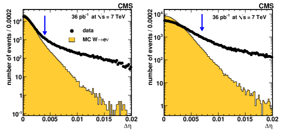
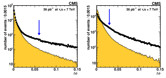
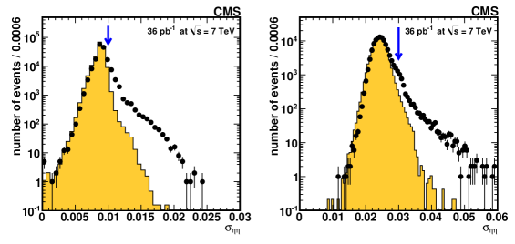
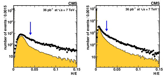
Figure 1: Distributions of the electron identification variables $\Delta\eta$, $\Delta\phi$, $\sigma_{\eta\eta}$, and $H/E$ for data (points with the error bars), for EB (left) and EE (right). For illustration the simulated $\mathrm{W}\rightarrow\mathrm{e}\nu$ signal (histograms), normalized to the number of events observed in data, is superimposed. These distributions are obtained after applying all the tight requirements on the selection variables, except that on the presented variable. The tight requirement on that variable is indicated with an arrow.

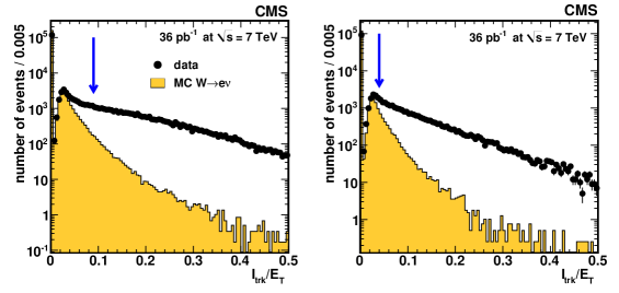
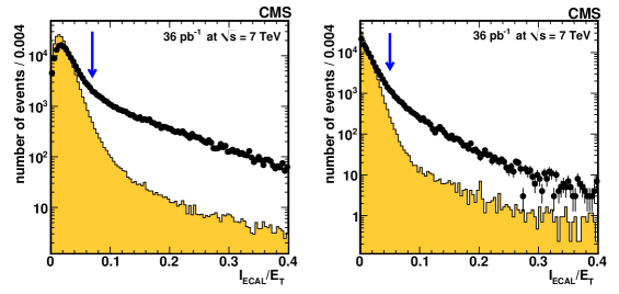
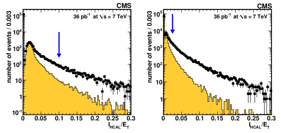
Figure 2: Distributions of the electron isolation variables $I_{\textrm{trk}}/E\,\,_{\!\!\!\mathrm{T}}$, $I_{\textrm{ECAL}}/E\,\,_{\!\!\!\mathrm{T}}$, and $I_{\textrm{HCAL}}/E\,\,_{\!\!\!\mathrm{T}}$ for data (points with the error bars), for EB (left) and EE (right). For illustration the simulated $\mathrm{W}\rightarrow\mathrm{e}\nu$ signal (histograms), normalized to the number of events observed in data, is superimposed. These distributions are obtained after applying all the tight requirements on the selection variables, except that on the presented variable. The tight requirement on that variable is indicated with an arrow.

The radiated photons may convert close to the original electron trajectory, leading to charge misidentification. Three different methods are used to determine the electron charge. First, the electron charge is determined by the signed curvature of the associated GSF track. Second, the charge is determined from the associated trajectory reconstructed in the silicon tracker using a Kalman Filter algorithm [36]. Third, the electron charge is determined based on the azimuthal angle between the vector joining the nominal interaction point and the ECAL cluster position and the vector joining the nominal interaction point and innermost hit of the GSF track. The electron charge is determined from the two out of three charge estimates that are in agreement. The electron charge misidentification rate is measured in data using the $\mathrm{Z}\rightarrow\mathrm{e}^{+}\mathrm{e}^{-}$ data sample to be within 0.1$\%$–1.3$\%$ in EB and 1.4$\%$–2.1$\%$ in EE, increasing with electron pseudorapidity.

Events are selected if they contain one or two electrons having $E\,\,_{\!\!\!\mathrm{T}}>25~{}\gev$ for the $\mathrm{W}\rightarrow\mathrm{e}\nu$ or the $\mathrm{Z}\rightarrow\mathrm{e}^{+}\mathrm{e}^{-}$ analysis, respectively. For the $\mathrm{Z}\rightarrow\mathrm{e}^{+}\mathrm{e}^{-}$ selection there is no requirement on the charges of the electrons. The energy of an electron candidate with $E\,\,_{\!\!\!\mathrm{T}}>25~{}\gev$ is determined by the ECAL cluster energy, while its momentum direction is determined by that of the associated track.

Particles misidentified as electrons are suppressed by requiring that the $\eta$ and $\phi$ coordinates of the track trajectory extrapolated to the ECAL match those of the ECAL cluster permitting only small differences ($\Delta\eta$, $\Delta\phi$) between the coordinates, by requiring a narrow ECAL cluster width in $\eta$ ($\sigma_{\eta\eta}$), and by limiting the ratio of the hadronic energy $H$ to the electromagnetic energy $E$ measured in a cone of $\Delta R=0.15$ around the ECAL cluster direction. More details on the electron identification variables can be found in Refs. [37, 38]. Electron isolation is based on requirements on the three isolation variables $I_{\textrm{HCAL}}/E\,\,_{\!\!\!\mathrm{T}}$, $I_{\textrm{ECAL}}/E\,\,_{\!\!\!\mathrm{T}}$, and $I_{\textrm{trk}}/E\,\,_{\!\!\!\mathrm{T}}$.

Electrons from photon conversions are suppressed by requiring the reconstructed electron track to have at least one hit in the innermost pixel layer. Furthermore, electrons are rejected when a partner track is found that is consistent with a photon conversion, based on the opening angle and the separation in the transverse plane at the point where the electron and partner tracks are parallel.

The electron selection criteria were obtained by optimizing signal and background levels according to simulation-based studies. The optimization was done for EB and EE separately.

Two sets of electron selection criteria are considered: a tight one and a loose one. Their efficiencies, from simulation studies based on $\mathrm{W}\rightarrow\mathrm{e}\nu$ events, are approximately 80$\%$ and 95$\%$, respectively. These efficiencies correspond to reconstructed electrons within the geometrical and kinematic acceptance, which is defined in Section 0.5. The tight selection criteria give a purer sample of prompt electrons and are used for both the $\mathrm{W}\rightarrow\mathrm{e}\nu$ and $\mathrm{Z}\rightarrow\mathrm{e}^{+}\mathrm{e}^{-}$ analyses. The virtue of this choice is to have consistent electron definitions for both analyses, simplifying the treatment of systematic uncertainties in the $\mathrm{W}/\mathrm{Z}$ ratio measurement. In addition, the tight working point, applied to both electrons in the $\mathrm{Z}\rightarrow\mathrm{e}^{+}\mathrm{e}^{-}$ analysis, reduces the QCD backgrounds to a negligible level. Distributions of the selection variables are shown in Figs. 1 and 2. The plots show the distribution of data together with the simulated signal normalized to the same number of events as the data, after applying all the tight requirements on the selection variables except the requirement on the displayed variable.

For the W analysis, an event is also rejected if there is a second electron that passes the loose selection with $E\,\,_{\!\!\!\mathrm{T}}>20~{}\gev$. This requirement reduces the contamination from DY events. The number of $\mathrm{W}\rightarrow\mathrm{e}\nu$ candidate events selected in the data sample is $235\,687$, with $132\,696$ positrons and $102\,991$ electrons.

For the Z analysis, two electrons are required within the ECAL acceptance, both with $E\,\,_{\!\!\!\mathrm{T}}>25~{}\gev$ and both satisfying the tight electron selection. Events in the dielectron mass region of $60<m_{\mathrm{ee}}<120$ GeV are counted. These requirements select $8452$ events.

0.4.3 Muon Channel Selection

Muons candidates are first reconstructed separately in the central tracker (referred to simply as “tracks” or “tracker tracks”) and in the muon detector (“stand-alone muons”). Stand-alone muons are then matched and combined with tracker tracks to form “global muons”. Another independent algorithm proceeds from the central tracker outwards, matching muon chambers hits and producing “tracker muons”.

The following quality selection are applied to muon candidates. Global and stand-alone muon candidates must have at least one good hit in the muon chambers. Tracker muons must match to hits in at least two muon stations. Tracks, global muons, and tracker muons must have more than 10 hits in the inner tracker, of which at least one must be in the pixel detector, and the impact parameter in the transverse plane, $d_{xy}$, calculated with respect to the beam axis, must be smaller than 2 mm. More details and studies on muon identification can be found in Refs. [39, 40].

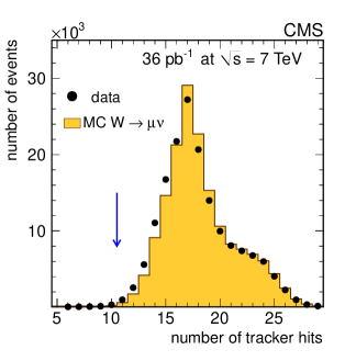
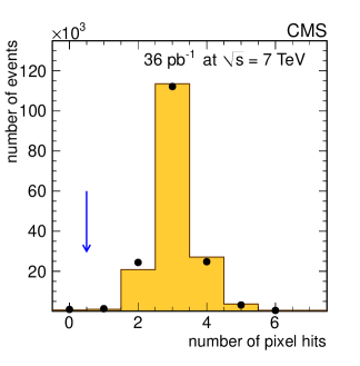
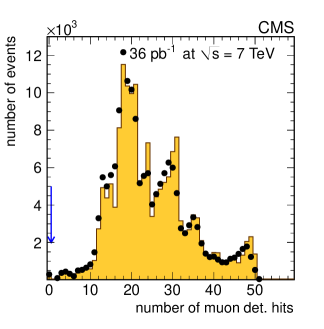
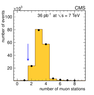
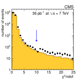
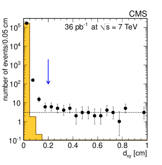
Figure 3: Distribution of number of hits in the inner tracker and in the pixel detector, number of hits in muon chambers, number of muon segments stations, $\chi^{2}$ per degree of freedom, and transverse impact parameter $d_{xy}$ for data (points with the error bars). For illustration the simulated $\mathrm{W}\rightarrow\mu\nu$ signal (histogram), normalized to the number of events observed in data, is superimposed. These distributions are for events satisfying all selection requirements, except that on the presented variable. The applied requirement on that variable is indicated as a blue arrow. In the $d_{xy}$ distribution, the horizontal line shows the average of the bins with $d_{xy}>0.2~{}\mathrm{cm}$ used to estimate the cosmic-ray muon contamination in the signal region. The excess of events in data in the region with $d_{xy}<0.2~{}\mathrm{cm}$ with respect to $\mathrm{W}\rightarrow\mu\nu$ signal simulation is due to muons from long-lived particle decays in the QCD background.

Muon candidates selected in the $\mathrm{W}\rightarrow\mu\nu$ analysis must be identified both as global and tracker muons. Moreover, as additional quality selection, the global muon fit must have a $\chi^{2}$ per degree of freedom less than 10 in order to reject misidentified muons and misreconstructed particles. The $\mathrm{W}\rightarrow\mu\nu$ candidate events must have a muon candidate in the fiducial volume $|\eta|<2.1$ with $p_{\mathrm{T}}>25~{}\GeV$. The muon must be isolated, satisfying $I^{\textrm{rel}}_{\textrm{comb}}=\left(I_{\textrm{trk}}+I_{\textrm{ECAL}}+I_{\textrm{HCAL}}\right)/p_{\mathrm{T}}<0.1$. Events containing a second muon with $p_{\mathrm{T}}>10~{}\GeV$ in the full muon acceptance region ($|\eta|<2.4$) are rejected to minimize the contamination from DY events. The distributions of the variables used for muon quality selection are shown in Fig. 3 after applying all selection requirements, except that on the presented variable.

Background due to a cosmic-ray muon crossing the detector in coincidence with a pp collision is very much reduced by the impact parameter requirement. The remaining cosmic-ray background is evaluated by extrapolating to the signal region the rate of events with large impact parameter. Figure 3 (bottom, right) shows the distribution of the impact parameter $d_{xy}$ for the $\mathrm{W}\rightarrow\mu\nu$ candidates satisfying all selection requirements, except that on $d_{xy}$. Candidates with large $d_{xy}$ are mainly due to cosmic-ray muons and their rate is independent of $d_{xy}$. A background fraction on the order of $10^{-4}$ in the $d_{xy}<2$ mm region is estimated.

The isolation distribution in data, together with the MC expectations, are shown in Fig. 4.

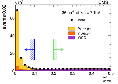
Figure 4: Distribution of $I^{\textrm{rel}}_{\textrm{comb}}$ for candidates with a good quality muon of $p_{\mathrm{T}}>25~{}\GeV$ in the fiducial region $|\eta|<2.1$. Points represent the data and the histograms the contribution from the different SM processes. The signal selection requirement (dark blue arrow, $I^{\textrm{rel}}_{\textrm{comb}}<0.1$) and the selection of the QCD-enriched control sample (light green arrow, $I^{\textrm{rel}}_{\textrm{comb}}>0.2$) are shown.

Events with $I^{\textrm{rel}}_{\textrm{comb}}>0.2$ are mainly from QCD multijet background, and are used as a control sample (Section 0.7.3).

After the selection process described, 166 457 events are selected, 97 533 of them with a positively charged muon candidate and 68 924 with a negatively charged muon candidate.

$\mathrm{Z}\rightarrow\MM$ candidate events are selected by pairing a global muon matched to an HLT trigger muon with a second oppositely charged muon candidate that can be either a global muon, a stand-alone muon, or a track. No $\chi^{2}$ selection or requirement that the muon be reconstructed through the tracker-muon algorithm is applied. The two muon candidates must both have $p_{\mathrm{T}}>20~{}\mathrm{GeV}$ and $|\eta|<2.1$, and their invariant mass must be in the range $60<m_{\mu\mu}<120$ $\mathrm{GeV}$. Both muon candidates must be isolated according to the tracker isolation requirement $I_{\textrm{trk}}<3$ GeV. The different choice of isolation requirements in $\mathrm{W}\rightarrow\mu\nu$ and $\mathrm{Z}\rightarrow\MM$ is motivated in Section 0.8.3. After the selection process, the number of selected events with two global muons is 13 728.

0.5 Acceptance

The acceptance $A_{\mathrm{W}}(\mathrm{e})$ for $\mathrm{W}\rightarrow\mathrm{e}\nu$ is defined as the fraction of simulated $\mathrm{W}$ events having an ECAL cluster within the ECAL fiducial volume with $E\,\,_{\!\!\!\mathrm{T}}>25\GeV$. The ECAL cluster must match the generated electron after final-state radiation (FSR) within a cone of $\Delta R=0.2$. No matching in energy is required.

There is an inefficiency in the ECAL cluster reconstruction for electrons direction within the ECAL fiducial volume due to a small fraction ($0.5\%$) of noisy or malfunctioning towers removed from the reconstruction. These are taken into account in the MC simulation, and no uncertainty is assigned to this purely geometrical inefficiency. The ECAL cluster selection efficiency is also affected by a bias in the electron energy scale due to the $25~{}\GeV$ energy threshold. The related systematic uncertainty is assigned to the final $\mathrm{W}$ and $\mathrm{Z}$ selection efficiencies.

The acceptance for the $\mathrm{Z}\rightarrow\mathrm{e}^{+}\mathrm{e}^{-}$ selection, $A_{\mathrm{Z}}(\mathrm{e})$, is defined as the number of simulated events with two ECAL clusters with $E\,\,_{\!\!\!\mathrm{T}}>25~{}\GeV$ within the ECAL fiducial volume and with invariant mass in the range $60<m_{\mathrm{ee}}<120\,\mathrm{GeV}$, divided by the total number of signal events in the same mass range, with the invariant mass evaluated using the momenta at generator level before FSR. The ECAL clusters must match the two simulated electrons after FSR within cones of $\Delta R<0.2$. No requirement on energy matching is applied.

For the $\mathrm{W}\rightarrow\mu\nu$ analysis, the acceptance $A_{\mathrm{W}}(\mu)$ is defined as the fraction of simulated $\mathrm{W}$ signal events with muons having transverse momentum $p_{\mathrm{T}}^{\textrm{gen}}$ and pseudorapidity $\eta^{\textrm{gen}}$, evaluated at the generator level after FSR, within the kinematic selection: $p_{\mathrm{T}}^{\textrm{gen}}>25~{}\GeV$ and $|\eta^{\textrm{gen}}|<2.1$.

The acceptance $A_{\mathrm{Z}}(\mu)$ for the $\mathrm{Z}\rightarrow\MM$ analysis is defined as the number of simulated $\mathrm{Z}$ signal events with both muons passing the kinematic selection with momenta evaluated after FSR, $p_{\mathrm{T}}^{\textrm{gen}}>20~{}\GeV$ and $|\eta^{\textrm{gen}}|<2.1$, and with invariant mass in the range $60<m_{\mu\mu}<120\,\mathrm{GeV}$, divided by the total number of signal events in the same mass range, with the invariant mass evaluated using the momenta at generator level before FSR.

Table 1 presents the acceptances for $\mathrm{W^{+}}$, $\mathrm{W^{-}}$, and inclusive $\mathrm{W}$ and $\mathrm{Z}$ events, computed from samples simulated with powheg using the CT10 PDF, for the muon and the electron channels. The acceptances are affected by several theoretical uncertainties, which are discussed in detail in Section 0.9.3.

Table 1: Acceptances from powheg (with CT10 PDF) for $\mathrm{W}\rightarrow\ell\nu$ and $\mathrm{Z}\rightarrow\ell^{+}\ell^{-}$ final states, with the MC statistics uncertainties.

Process	$A_{\mathrm{W,Z}}$
	$\ell=\mathrm{e}$	$\ell=\mu$
$\mathrm{W^{+}}\rightarrow\ell^{+}\nu$	$0.5017\pm 0.0004$	$0.4594\pm 0.0004$
$\mathrm{W^{-}}\rightarrow\ell^{-}\overline{\nu}$	$0.4808\pm 0.0004$	$0.4471\pm 0.0004$
$\mathrm{W}\rightarrow\ell\nu$	$0.4933\pm 0.0003$	$0.4543\pm 0.0003$
$\mathrm{Z}\rightarrow\ell^{+}\ell^{-}$	$0.3876\pm 0.0005$	$0.3978\pm 0.0005$

0.6 Efficiencies

A key component of this analysis is the estimation of lepton efficiencies. The efficiency is determined for different selection steps:

• offline reconstruction of the lepton;

• lepton selection, with identification and isolation criteria;

• trigger (L1+HLT).

The order of the above selections steps is important. Lepton efficiency for each selection is determined with respect to the prior step.

A tag-and-probe (T&P) technique is used, as described below, on pure samples of $\mathrm{Z}\rightarrow\ell^{+}\ell^{-}$ events. The statistical uncertainty on the efficiencies is ultimately propagated as a systematic uncertainty on the cross-section measurements. This procedure has the advantage of extracting the efficiencies from a sample of leptons kinematically very similar to those used in the $\mathrm{W}$ analysis and exploits the relatively pure selection of $\mathrm{Z}\rightarrow\ell^{+}\ell^{-}$ events obtained after a dilepton invariant mass requirement around the Z mass.

The T&P method is as follows: one lepton candidate, called the “tag”, satisfies trigger criteria, tight identification and isolation requirements. The other lepton candidate, called the “probe”, is required to pass specific criteria that depend on the efficiency under study.

For each kind of efficiency, the T&P method is applied to real data and to simulated samples, and the ratio of efficiencies in data ($\epsilon_{\mathrm{data}}$) and simulation ($\epsilon_{\mathrm{sim}}$) is computed:

$$\rho=\frac{\epsilon_{\mathrm{data}}}{\epsilon_{\mathrm{sim}}}\,,$$ (1)

together with the associated statistical and systematic uncertainties.

0.6.1 Electrons

As mentioned in the previous section, the tight electron selection is considered for both the W and Z analyses, so:

$$\epsilon_{\textrm{all}}=\epsilon_{\textrm{rec}}\,\epsilon_{\textrm{tight}}\,\epsilon_{\textrm{trg}}.$$ (2)

The reconstruction efficiency $\epsilon_{\textrm{rec}}$ is relative to ECAL clusters within the ECAL acceptance, the selection efficiency $\epsilon_{\textrm{tight}}$ is relative to GSF electrons within the acceptance, and the trigger efficiency $\epsilon_{\textrm{trg}}$ is relative to electrons satisfying the tight selection criteria.

All the efficiencies are determined by the T&P technique. Selections with different criteria have been tried on the tag electron. It was found that the estimated efficiencies are insensitive to the tag selection definition. The invariant mass of the T&P pair is required to be within the window $60<m_{\mathrm{ee}}<120~{}\GeV$, ensuring high purity of the probe sample. No opposite-charge requirement is enforced.

The number of probes passing and failing the selection is determined from fits to the invariant mass distribution, with signal and background components. Estimated backgrounds, mostly from QCD multijet processes, are in most cases at the percent level of the overall sample, but can be larger in subsamples where the probe fails a selection, hence the importance of background modeling. The signal shape is a Breit–Wigner with nominal Z mass and width convolved with an asymmetric resolution function (Crystal Ball [41]) with floating parameters. The background is modeled by an exponential. Systematic uncertainties that depend on the efficiency under study are determined by considering alternative signal and background shape models. Details can be found in Section 0.9.

The T&P event selection efficiencies in the simulation are determined from large samples of signal events with no background added.

The T&P efficiencies are measured for the EB and EE electrons separately. Tag-and-probe efficiencies are also determined separately by charge, to be used in the measurements of the W⁺ and W^- cross sections and their ratio. Inclusive efficiencies and correction factors are summarized in Table 2. The T&P measurements of the efficiencies on the right-hand side of Eq. (2) are denoted as $\epsilon_{\textrm{t\&p-rec}}$, $\epsilon_{\textrm{t\&p-tight}}$, and $\epsilon_{\textrm{t\&p-trg}}$.

Table 2: Tag-and-probe efficiencies in data and simulation, and the correction factors used in the electron channels for the barrel (EB) and endcaps (EE). The combined statistical and systematic uncertainties are quoted.

Efficiency	Data	Simulation	Data/simulation ($\rho$)
EB
$\epsilon_{\textrm{t\&p-rec}}$	$({97.0}\pm{1.0})\%$	$({97.78}\pm{0.02})\%$	$0.992\pm 0.011$
$\epsilon_{\textrm{t\&p-tight}}$	$({84.0}\pm{0.3})\%$	$({87.47}\pm{0.05})\%$	$0.960\pm 0.004$
$\epsilon_{\textrm{t\&p-trg}}$	$({98.0}\pm{0.1})\%$	$({97.10}\pm{0.03})\%$	$1.009\pm 0.001$
$\epsilon_{\textrm{t\&p-all}}$	$({79.8}\pm{0.9})\%$	$({83.05}\pm{0.06})\%$	$0.961\pm 0.011$
EE
$\epsilon_{\textrm{t\&p-rec}}$	$({94.3}\pm{1.1})\%$	$({94.61}\pm{0.05})\%$	$0.997\pm 0.011$
$\epsilon_{\textrm{t\&p-tight}}$	$({73.1}\pm{0.7})\%$	$({75.61}\pm{0.06})\%$	$0.966\pm 0.009$
$\epsilon_{\textrm{t\&p-trg}}$	$({97.3}\pm{0.3})\%$	$({97.16}\pm{0.04})\%$	$1.001\pm 0.003$
$\epsilon_{\textrm{t\&p-all}}$	$({67.0}\pm{1.0})\%$	$({69.51}\pm{0.07})\%$	$0.965\pm 0.015$

Event selection efficiencies are measured with respect to the W events within the ECAL acceptance. Simulation efficiencies estimated from POWHEG $\mathrm{W}$ samples are shown in Table 3. These are efficiencies at the event level, e.g.: they include efficiency loss due to the second electron veto. Given the acceptances listed in Table 1 and the T&P efficiencies listed in Table 2, the overall efficiency correction factors for electrons from $\mathrm{W}$ decays are computed. The overall $\mathrm{W}$ signal efficiencies, obtained as products of simulation efficiencies with data/simulation correction factors, are listed in Table 3.

Table 3: Simulation efficiencies and the final corrected selection efficiencies for the $\mathrm{W^{+}}$, $\mathrm{W^{-}}$, and their average, in the $\mathrm{W}\rightarrow\mathrm{e}\nu$ analysis. The quoted uncertainties are statistical for $\epsilon_{\mathrm{sim}}$ and include both statistical and systematic uncertainties for the corrected efficiencies $\epsilon_{\mathrm{sim}}\times\rho$.

	$\epsilon_{\mathrm{sim}}$	$\epsilon_{\mathrm{sim}}\times\rho$
$\mathrm{W^{+}}\rightarrow\mathrm{e}^{+}\nu$	$(76.04\pm 0.03)\%$	$({73.7}\pm{1.0})\%$
$\mathrm{W^{-}}\rightarrow\mathrm{e}^{-}\overline{\nu}$	$(76.94\pm 0.03)\%$	$({73.2}\pm{1.0})\%$
$\mathrm{W}\rightarrow\mathrm{e}\nu$	$(76.40\pm 0.02)\%$	$({73.5}\pm{0.9})\%$

The efficiencies and the data/simulation ratios are also estimated in bins of the electron $E\,\,_{\!\!\!\mathrm{T}}$ and $\eta$ in order to examine in detail the detector performance and take into account the differences in the W and Z kinematic distributions. The data/simulation ratios for reconstruction, selection, and trigger are shown in Fig. 5 as functions of the electron $E\,\,_{\!\!\!\mathrm{T}}$ and $\eta$.

The reconstruction data/simulation ratios appear to be uniform with respect to $E\,\,_{\!\!\!\mathrm{T}}$ and $\eta$, so a smaller number of bins is sufficient for the determination of their values. The data/simulation ratios for the selection and trigger efficiencies show a dependence that is estimated using ten $\eta$ bins and six $E\,\,_{\!\!\!\mathrm{T}}$ bins. Data/simulation ratios are estimated for both electron charges as well.

The binned ratios and simulation efficiencies are transferred into the W analysis by properly weighting their product in each ($E\,\,_{\!\!\!\mathrm{T}}$, $\eta$) bin by the relative ECAL cluster abundance estimated from POWHEG simulations. The corrected efficiencies are compared with the two-bin case in which the efficiencies are estimated in two bins of $\eta$ (EB and EE). The multibin corrected efficiencies are found to be consistent with the two-bin corrected efficiencies within the assigned uncertainties. In order to be sure that no hidden systematic uncertainty is missed, half of the maximum difference between the multibin and two-bin corrected efficiencies is propagated as an additional systematic uncertainty on the two-bin efficiencies used to estimate the cross sections. The additional relative uncertainty is at the level of 0.6$\%$.

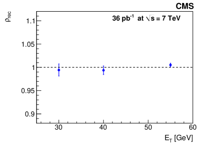
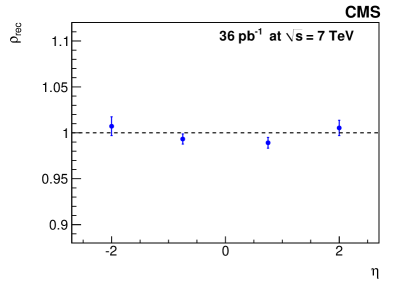
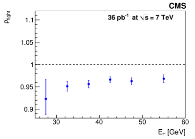
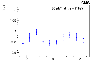
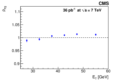
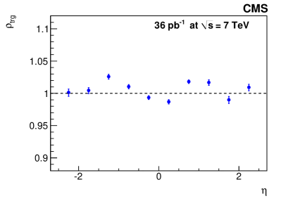
Figure 5: Data/simulation T&P ratios versus electron $E\,\,_{\!\!\!\mathrm{T}}$ (left column) and $\eta$ (right column). The ratios are presented for the reconstruction ($\rho_{\mathrm{rec}}$, top row), selection ($\rho_{\mathrm{tight}}$, middle row), and trigger ($\rho_{\mathrm{trg}}$, bottom row) efficiencies. Points with error bars represent the ratio measured in data; dashed lines correspond to a constant ratio of one.

The $\mathrm{Z}$ selection efficiencies for data and simulation are obtained based on the T&P efficiencies listed in Table 2 and the event acceptances given in Table 1. The $\mathrm{Z}$ efficiencies are first determined after reconstruction and identification (as products of single-electron efficiencies). The event trigger efficiency is computed as the probability that at least one of the two electrons satisfies the L1+HLT requirement. The overall selection efficiency for the $\mathrm{Z}$ analysis is the product of the reconstruction, identification, and trigger efficiencies. The simulation efficiency obtained from the POWHEG $\mathrm{Z}$ samples, together with the final corrected $\mathrm{Z}$ selection efficiency $\epsilon_{\mathrm{sim}}\times\rho$, are shown in Table 4. These efficiencies are relative to the $\mathrm{Z}$ events with both electrons within the ECAL acceptance.

Table 4: Simulation efficiency and the final corrected selection efficiency for the  $\mathrm{Z}\rightarrow\mathrm{e}^{+}\mathrm{e}^{-}$ analysis. The quoted uncertainties are statistical for $\epsilon_{\mathrm{sim}}$ and include both statistical and systematic uncertainties for the corrected efficiency $\epsilon_{\mathrm{sim}}\times\rho$.

	$\epsilon_{\mathrm{sim}}$	$\epsilon_{\mathrm{sim}}\times\rho$
$\mathrm{Z}\rightarrow\mathrm{e}^{+}\mathrm{e}^{-}$	$({66.74}\pm{0.07})\%$	$({60.9}\pm{1.1})\%$

0.6.2 Muons

For the $\mathrm{W}\rightarrow\mu\nu$ cross section determination the single-muon efficiency combines the efficiencies of all the steps in the muon selection: triggering on the muon, reconstructing it in the muon and central detectors, and applying the quality selection and the isolation requirement. In the procedure followed in this analysis, the reconstruction efficiency in the central tracker is factorized and computed independently, while the remaining terms are computed globally, without further factorizing them into different terms.

An initial preselection of Z events for the T&P method is performed by selecting events that contain tracks measured in the central tracker having $p_{\mathrm{T}}>25$ GeV, $|\eta|<2.1$, and, when combined with an oppositely charged track, give an invariant mass in the range $60<m_{\mu^{+}\mu^{-}}<120$ GeV. We further require the presence in the event of a “tag” muon, defined as a global muon, that is matched to one of the preselected tracks, passes the selection described in Section 0.4.3, and corresponds to an HLT muon. The number of tag muons selected in data is about $22\,000$. All the other preselected tracks are considered as probes to evaluate the muon efficiency. The background present in this sample is subtracted with a fit to the dimuon invariant mass spectrum of the sum of a Z component and a linear background contribution. The shape of the Z component is taken from simulation.

The efficiency is studied as a function of the muon $\eta$ and $p_{\mathrm{T}}$. A dependence on $\eta$ is observed (Fig. 6, left) because different regions are covered by different muon detectors. This behavior is not fully reproduced in the simulation, as reflected in the corresponding $\rho$ values (Fig. 6, right). The efficiency also exhibits a dependence on $p_{\mathrm{T}}$ (Fig. 7, left), but this trend is similar in data and in simulation, and the correction factors can be taken as approximately constant up to $p_{\mathrm{T}}$ = 100 GeV (Fig. 7, right). These binned correction factors are applied to the W analysis during signal modeling (Section 8): W simulated events are weighted with the $\rho$ factor corresponding to the ($p_{\mathrm{T}}$, $\eta$) bin of the muon. The slightly difference between the kinematic characteristics of the muons and those from W decays is thus taken into account.

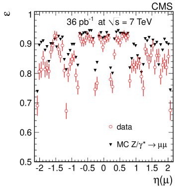
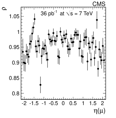
Figure 6: Single-muon efficiencies (left) for data (red circles with error bars) and simulation (black triangles), and the ratio between them (right), as a function of the muon $\eta$.

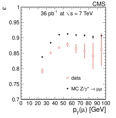
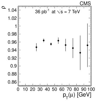
Figure 7: Single-muon efficiencies (left) for data (red circles with error bars) and simulation (black triangles) and the ratio between them (right), as a function of the muon $p_{\mathrm{T}}$.

The average single-muon efficiencies and correction factors are reported in Table 5 for positively and negatively charged muons separately, and inclusively. The statistical uncertainties reflect the size of the available Z sample. Systematic uncertainties on $\epsilon_{\mathrm{t\&p}}(\mathrm{data})$ and the correction factors $\rho$ are discussed in Section 0.9.2.

Table 5: Tag-and-probe efficiencies in data and simulation and correction factors for positively and negatively charged muons. The errors on $\epsilon_{\mathrm{t\&p}}(\mathrm{sim)}$ are statistical only, while the systematic uncertainty is included for the other quantities.

	$\mu^{+}$	$\mu^{-}$	$\mu^{\pm}$
$\epsilon_{\mathrm{t\&p}}(\mathrm{data})$	$(86.0\pm 0.8)\%$	$(85.0\pm 0.8)\%$	$(85.58\pm 0.8)\%$
$\epsilon_{\mathrm{t\&p}}(\mathrm{sim)}$	$(89.25\pm 0.05)\%$	$(89.38\pm 0.05)\%$	$(89.32\pm 0.04)\%$
$\rho$	$(96.3\pm 0.9)\%$	$(95.1\pm 0.9)\%$	$(95.7\pm 0.9)\%$

A small fraction of muon events are lost because of L1 muon trigger prefiring, i.e., the assignment of a muon segment to an incorrect bunch crossing, occurring with a probability of a few per mille per segment. The effect is only sizable in the drift-tube system. The efficiency correction in the barrel region is estimated for the current data to be ${\sim}1\%$ per muon. This estimate is obtained from studies of muon pairs selected by online and offline single-muon trigger paths at the wrong bunch crossing, that have an invariant mass near the Z mass. Tracker information is not present in the case of prefiring, precluding the building of a trigger muon online or a global muon in the offline reconstruction. Since this effect is not accounted for in the efficiency from T&P, the measured $\mathrm{Z}\rightarrow\MM$ and $\mathrm{W}\rightarrow\mu\nu$ cross sections are increased by 1% and 0.5%, respectively (including barrel and endcap regions) to correct for the effect of trigger prefiring. The uncertainty on those corrections is taken as a systematic uncertainty.

The $\mathrm{W}\rightarrow\mu\nu$ efficiencies from simulation are shown in Table 6 for the $\mathrm{W^{+}}$ and $\mathrm{W^{-}}$ samples separately and combined after applying the binned corrections estimated with the T&P method using Z events.

Table 6: Simulation efficiencies and final corrected efficiencies for the $\mathrm{W}\rightarrow\mu\nu$ analysis. The quoted uncertainties are statistical for $\epsilon_{\mathrm{sim}}$ and include both statistical and systematic uncertainties for the corrected efficiencies $\epsilon_{\mathrm{sim}}\times\rho$.

	$\epsilon_{\mathrm{sim}}$	$\epsilon_{\mathrm{sim}}\times\rho$
$\mathrm{W^{+}}\rightarrow\mu^{+}\nu$	$(89.19\pm 0.03)\%$	$(85.4\pm 0.8)\%$
$\mathrm{W^{-}}\rightarrow\mu^{-}\overline{\nu}$	$(89.19\pm 0.03)\%$	$(84.1\pm 0.8)\%$
$\mathrm{W}\rightarrow\mu\nu$	$(89.19\pm 0.03)\%$	$(84.8\pm 0.8)\%$

For the $\mathrm{Z}\rightarrow\MM$ cross section measurement, the muon efficiencies are determined together with the Z yield using a simultaneous fit described in Section 0.8.3.

0.7 The $\mathrm{W}\rightarrow\ell\nu$ Signal Extraction

The signal and background yields are obtained by fitting the ${E\!\!\!/}_{\!\mathrm{T}}$ distributions for $\mathrm{W}\rightarrow\mathrm{e}\nu$ and $\mathrm{W}\rightarrow\mu\nu$ to different functional models. An accurate ${E\!\!\!/}_{\!\mathrm{T}}$ measurement is essential for distinguishing a $\PW$ signal from QCD multijet backgrounds. We profit from the application of the PF algorithm, which provides superior ${E\!\!\!/}_{\!\mathrm{T}}$ reconstruction performance [42] with respect to alternative algorithms at the energy scale of the $\PW$ boson.

The ${E\!\!\!/}_{\!\mathrm{T}}$ is the magnitude of the transverse component of the missing momentum vector, computed as the negative of the vector sum of all reconstructed transverse momenta of particles identified with the PF algorithm. The algorithm combines the information from the inner tracker, the muon chambers, and the calorimeters to classify reconstructed objects according to particle type (electron, muon, photon, or charged or neutral hadron), thereby allowing precise energy corrections. The use of the tracker information reduces the sensitivity of ${E\!\!\!/}_{\!\mathrm{T}}$ to miscalibration of the calorimetry.

The QCD multijet background is one of the most significant backgrounds in W analyses. At high ${E\!\!\!/}_{\!\mathrm{T}}$, EWK backgrounds, in particular $\mathrm{W}\rightarrow\tau\nu$ and DY, also become relevant, leading to contamination levels on the order of $10\%$.

The ${E\!\!\!/}_{\!\mathrm{T}}$ model is fitted to the observed distribution as the sum of three contributions: the W signal, and the QCD and EWK backgrounds. The EWK contributions are normalized to the W signal yield in the fit through the ratios of the theoretical cross sections.

Simultaneous fits are performed to the two ${E\!\!\!/}_{\!\mathrm{T}}$ spectra of W⁺ and W^- candidates, fitting either the total W cross section and the ratio of positive and negative W cross sections, or the individual positive and negative W cross sections. In both cases the overall normalization of QCD multijet events is determined from the fit. The diboson and $\mathrm{t}\bar{\mathrm{t}}$ contributions, taken from simulations, are negligible (Section 0.7.2).

In the following sections the modeling of the ${E\!\!\!/}_{\!\mathrm{T}}$ shape for the signal and the EWK backgrounds are presented, and the methods used to determine the ${E\!\!\!/}_{\!\mathrm{T}}$ shape for the QCD multijet background from data are described. Finally, the extraction of the signal yields is discussed.

0.7.1 Signal ${E\!\!/}_{\!\mathrm{T}}$ Modeling

The $\mathrm{W}\rightarrow\ell\nu$ signal is extracted with methods that employ simulation predictions of the ${E\!\!\!/}_{\!\mathrm{T}}$ distribution in signal events. These predictions rely on the modeling of the vector-boson recoil and detector effects that can be difficult to simulate accurately. Discrepancies could result from deficiencies in the modeling of the calorimeter response and resolution, and from an incomplete description of the underlying event. These residual effects are addressed using corrections determined from the study of Z-boson recoil in data, discussed in the following paragraph.

The recoil to the vector boson is defined as the negative of the vector sum of transverse energy vectors of all particles reconstructed with the PF algorithm in W and Z events, after subtracting the contribution from the daughter lepton(s). The recoil is determined for each event in $\mathrm{Z}\rightarrow\ell^{+}\ell^{-}$ data and simulated $\mathrm{Z}\rightarrow\ell^{+}\ell^{-}$ and $\mathrm{W}\rightarrow\ell\nu$ samples. We fit the distributions of the recoil components (parallel and perpendicular to the boson p_T direction) with a double Gaussian, whose mean and width vary with the boson transverse momentum. For each sample, we fit polynomials to the extracted mean and width of the recoil distributions as functions of the boson transverse momentum. The ratios of data to simulation fit-parameters from the $\mathrm{Z}$ samples are used as scale factors to correct the polynomials parameters of the W simulated recoil curves. For each $\mathrm{W}$ simulated event, the recoil is replaced with a value drawn from the distribution obtained with the corrected parameters corresponding to the $\mathrm{W}$ p_T. The ${E\!\!\!/}_{\!\mathrm{T}}$ value is calculated by adding back the energy of the $\mathrm{W}$ lepton. The energy of the lepton used in the calculation is corrected for the energy-scale and resolution effects. Statistical uncertainties from the fits are propagated into the ${E\!\!\!/}_{\!\mathrm{T}}$ distribution as systematic uncertainties. An additional systematic uncertainty is included to account for possible differences in the recoil behavior of the W and Z bosons.

The same strategy is followed for the recoil corrections in the electron and muon analyses. As an example, Fig. 8 (left) shows the effect of the recoil corrections on the ${E\!\!\!/}_{\!\mathrm{T}}$ shape for simulated events in the electron channel, while Fig. 8 (right) shows the uncertainty from the recoil method propagated to the corrected ${E\!\!\!/}_{\!\mathrm{T}}$ shape of $\mathrm{W}\rightarrow\mathrm{e}\nu$ events. The distribution of the residuals, $\chi$, is shown at the bottom of each plot, where $\chi$ is defined as the per-bin difference of the two distributions, divided by the corresponding statistical uncertainty. The same definition is used throughout this paper.

The systematic uncertainties on the signal ${E\!\!\!/}_{\!\mathrm{T}}$ shape are propagated as systematic uncertainties on the extracted signal yield through the fitting procedure. Signal shapes are determined for the W⁺ and W^- separately.

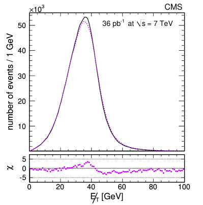
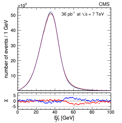
Figure 8: Left: simulated ${E\!\!\!/}_{\!\mathrm{T}}$ distribution in $\mathrm{W}\rightarrow\mathrm{e}\nu$ events before (continuous black line) and after (dashed red line) recoil corrections. Right: the uncertainties from the recoil method propagated to the corrected ${E\!\!\!/}_{\!\mathrm{T}}$ shape of $\mathrm{W}\rightarrow\mathrm{e}\nu$ events (continuous black line, identical to the dashed red line on the left-hand side plot) are presented with the red-dashed and blue-dotted lines. These two shapes are obtained when the recoil systematic uncertainties are varied by one standard deviation. At the bottom of each plot is shown the distribution of the residuals, $\chi$, defined as the per-bin difference of the two distributions, divided by the corresponding statistical uncertainty.

0.7.2 Electroweak Backgrounds

A certain fraction of the events passing the selection criteria for $\mathrm{W}\rightarrow\ell\nu$ are due to other EWK processes. Several sources of contamination have been identified. The events with $\mathrm{Z}\rightarrow\ell^{+}\ell^{-}$ (DY background), where one of the two leptons lies beyond the detector acceptance and escapes detection, mimic the signature of $\mathrm{W}\rightarrow\ell\nu$ events. Events from $\mathrm{Z}\rightarrow\tau^{+}\tau^{-}$ and $\mathrm{W}\rightarrow\tau\nu$, with the tau decaying leptonically, have in general a lower-momentum lepton than signal events and are strongly suppressed by the minimum $p_{\mathrm{T}}$ requirements.

The ${E\!\!\!/}_{\!\mathrm{T}}$ shape for the EWK vector boson and ${\mathrm{t}}\bar{\mathrm{t}}$ contributions are evaluated from simulations. For the main EWK backgrounds ($\mathrm{Z}\rightarrow\ell^{+}\ell^{-}$ and $\mathrm{W}\rightarrow\tau\nu$), the ${E\!\!\!/}_{\!\mathrm{T}}$ shape is corrected by means of the procedure described in Section 0.7.1. The ${E\!\!\!/}_{\!\mathrm{T}}$ shapes are evaluated separately for $\mathrm{W^{+}}\rightarrow\tau^{+}\nu$ and $\mathrm{W^{-}}\rightarrow\tau^{-}\overline{\nu}$.

A summary of the background fractions in the $\mathrm{W}\rightarrow\mathrm{e}\nu$ and $\mathrm{W}\rightarrow\mu\nu$ analyses can be found in Table 7. The fractions are similar for the $\mathrm{W}\rightarrow\mathrm{e}\nu$ and $\mathrm{W}\rightarrow\mu\nu$ channels, except for the DY background which is higher in the $\mathrm{W}\rightarrow\mathrm{e}\nu$ channel. The difference is mainly due to the tighter definition of the DY veto in the $\mathrm{W}\rightarrow\mu\nu$ channel, which is not compensated by the larger geometrical acceptance of electrons ($|\eta|<2.5$) with respect to muons ($|\eta|<2.1$).

Table 7: Estimated background-to-signal ratios in the $\mathrm{W}\rightarrow\mathrm{e}\nu$ and $\mathrm{W}\rightarrow\mu\nu$ channels.

Processes	Bkg. to sig. ratio
	$\mathrm{W}\rightarrow\mathrm{e}\nu$	$\mathrm{W}\rightarrow\mu\nu$
$\mathrm{Z}\rightarrow\mathrm{e}^{+}\mathrm{e}^{-},\,\mu^{+}\mu^{-},\,\tau^{+}\tau^{-}$ (DY)	7.6%	4.6%
$\mathrm{W}\rightarrow\tau\nu$	3.0%	$3.0$%
$\mathrm{W}\mathrm{W}$+$\mathrm{W}\mathrm{Z}$+$\mathrm{Z}\mathrm{Z}$	0.1%	$0.1$%
$\mathrm{t}\bar{\mathrm{t}}$	0.4%	$0.4$%
Total EWK	11.2%	$8.1$%

0.7.3 Modeling of the QCD Background and $\mathrm{W}\rightarrow\mathrm{e}\nu$ Signal Yield

Three signal extraction methods are used, which give consistent signal yields. The method described in Section 0.7.3 is used to extract the final result.

Modeling the QCD Background Shape with an Analytical Function

The $\mathrm{W}\rightarrow\mathrm{e}\nu$ signal is extracted using an unbinned maximum likelihood (UML) fit to the ${E\!\!\!/}_{\!\mathrm{T}}$ distribution.

The shape of the ${E\!\!\!/}_{\!\mathrm{T}}$ distribution for the QCD background is modeled by a parametric function (modified Rayleigh distribution) whose expression is

$$f_{\mathrm{CQD}}({E\!\!\!/}_{\!\mathrm{T}})={E\!\!\!/}_{\!\mathrm{T}}\exp\left(-\frac{{E\!\!\!/}_{\!\mathrm{T}}{{}^{2}}}{2(\sigma_{0}+\sigma_{1}{E\!\!\!/}_{\!\mathrm{T}})^{2}}\right)\,.$$ (3)

The fit to a control sample, defined by inverting the track-cluster matching selection variables $\Delta\eta$, $\Delta\phi$, shown in Fig. 9, illustrates the quality of the description of the background shape by the parameterized function, including the region of the signal, at high ${E\!\!\!/}_{\!\mathrm{T}}$.

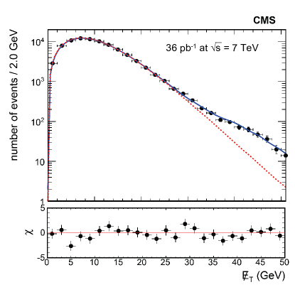
Figure 9: Fit to the background-dominated control sample defined by inverting the selection on the track-match variables, while maintaining the rest of the signal selection. The blue solid line represents the model used to fit the control data sample. This is a Rayleigh function plus a floating-yield signal shape that accounts for the signal contamination in the control region. The magenta dashed line shows the Rayleigh function alone with its parameters estimated from the combined fit.

To study the systematic uncertainties associated with the background shape, the resolution term in Eq. (3) was changed by introducing an additional QCD shape parameter $\sigma_{2}$, thus: $\sigma_{0}+\sigma_{1}{E\!\!\!/}_{\!\mathrm{T}}+\sigma_{2}{E\!\!\!/}_{\!\mathrm{T}}^{2}$.

The free parameters of the UML fit are the QCD background yield, the $\mathrm{W}$ signal yield, and the background shape parameters $\sigma_{0}$ and $\sigma_{1}$. The following signal yields are obtained: $136\,328\pm 386$ for the inclusive sample, $81\,568\pm 297$ for the $\mathrm{W^{+}}\rightarrow\mathrm{e}^{+}\nu$ sample, and $54\,760\pm 246$ for the $\mathrm{W^{-}}\rightarrow\mathrm{e}^{-}\overline{\nu}$ sample. The fit to the inclusive $\mathrm{W}\rightarrow\mathrm{e}\nu$ sample is displayed in Fig. 10, while the fits for the charge-specific channels are displayed in Fig. 11.

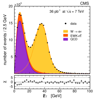
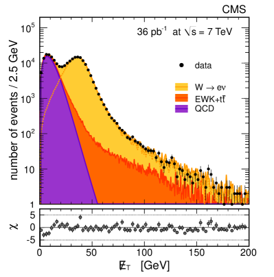
Figure 10: The ${E\!\!\!/}_{\!\mathrm{T}}$ distribution for the selected $\mathrm{W}\rightarrow\mathrm{e}\nu$ candidates on a linear scale (left) and on a logarithmic scale (right). The points with the error bars represent the data. Superimposed are the contributions obtained with the fit for QCD background (violet, dark histogram), all other backgrounds (orange, medium histogram), and signal plus background (yellow, light histogram). The orange dashed line is the fitted signal contribution.

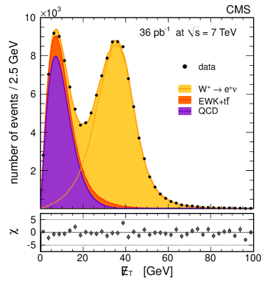
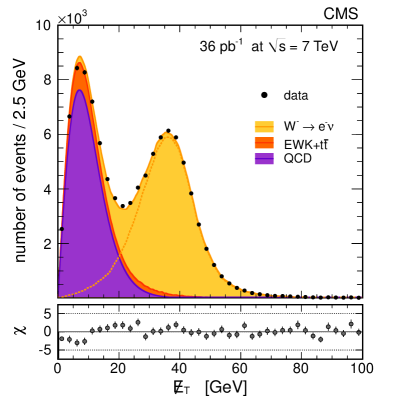
Figure 11: The ${E\!\!\!/}_{\!\mathrm{T}}$ distributions for the selected W⁺ (left) and W^- (right) candidates. The points with the error bars represent the data. Superimposed are the contributions obtained with the fit for QCD background (violet, dark histogram), all other backgrounds (orange, medium histogram), and signal plus background (yellow, light histogram). The orange dashed line is the fitted signal contribution.

The Kolmogorov–Smirnov probabilities for the fits to the charge-specific channels are $0.31$ for the $\mathrm{W^{+}}$ sample and $0.25$ for the $W^{-}$ sample.

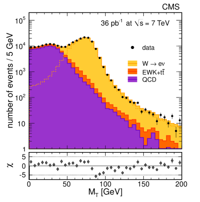
Figure 12: The $M_{\mathrm{T}}$ distribution for the selected $\mathrm{W}\rightarrow\mathrm{e}\nu$ candidates on a linear scale (left) and on a logarithmic scale (right). The points with the error bars represent the data. Superimposed are the contributions obtained with the fit for QCD background (violet, dark histogram), all other backgrounds (orange, medium histogram), and signal plus background (yellow, light histogram). The orange dashed line is the fitted signal contribution.

Figure 12 shows the distribution for the inclusive $\mathrm{W}$ sample of the transverse mass, defined as $M_{\mathrm{T}}=\sqrt{2p_{\mathrm{T}}{E\!\!\!/}_{\!\mathrm{T}}(1-\cos(\Delta\phi_{\mathrm{l},{E\!\!\!/}_{\!\mathrm{T}}}))}$, where $\Delta\phi_{\mathrm{l},{E\!\!\!/}_{\!\mathrm{T}}}$ is the azimuthal angle between the lepton and the ${E\!\!\!/}_{\!\mathrm{T}}$ directions.

Modeling the QCD Background Shape with a Fixed Distribution

In this approach the QCD shape is extracted directly from data using a control sample obtained by inverting a subset of the requirements used to select the signal. After fixing the shape from data, only the normalization is allowed to float in the fit.

The advantage of this approach is that detector effects, such as anomalous signals in the calorimeters or dead ECAL towers, are automatically reproduced in the QCD shape, since these effects are not affected by the selection inversion used to define the control sample. The track-cluster matching variable $\Delta\eta$ is found to have the smallest correlation with ${E\!\!\!/}_{\!\mathrm{T}}$ and is therefore chosen as the one to invert in order to remove the signal and obtain the QCD control sample. Requirements on isolation and $H/E$ are the same as for the signal selection since these variables show significant correlation with ${E\!\!\!/}_{\!\mathrm{T}}$.

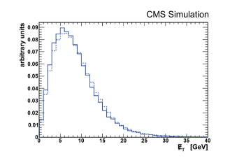
Figure 13: Normalised ${E\!\!\!/}_{\!\mathrm{T}}$ distribution for QCD and $\gamma$+jet simulated events passing the signal selection (solid histogram) compared to the normalised distribution for events from all simulated samples passing the same inverted selection criteria used to obtain the control sample in data (dashed histogram).

The shape of the ${E\!\!\!/}_{\!\mathrm{T}}$ distribution for QCD and $\gamma$+jet simulated events passing the signal selection is compared to the ${E\!\!\!/}_{\!\mathrm{T}}$ distribution for a simulated control sample composed of all simulated samples (signal and all backgrounds, weighted according to the theoretical production cross sections), after applying the same anti-selection as in data (Fig. 13).

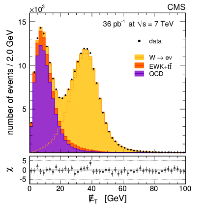
Figure 14: Result of the fixed-shape fit to the ${E\!\!\!/}_{\!\mathrm{T}}$ distribution for all W candidates. The points with the error bars represent the data. Superimposed are the results of the maximum likelihood fit for QCD background (violet, dark histogram), other backgrounds (orange, medium histogram), and signal plus background (yellow, light histogram). The orange dashed line (left plot) is the fit contribution from signal.

The difference in the ${E\!\!\!/}_{\!\mathrm{T}}$ distributions from the signal and inverted selections is found to be predominantly due to two effects, which can be reduced by applying corrections. The first effect is due to a large difference in the distribution of the output of a multivariate analysis (MVA) used for electron identification in the PF algorithm, between the selected events and the control sample. The value of the MVA output determines whether an electron candidate is treated by the PF algorithm as a genuine electron, or as a superposition of a charged pion and a photon, with track momentum and cluster energy each contributing separately to ${E\!\!\!/}_{\!\mathrm{T}}$. The control sample contains a higher fraction of electron candidates in the latter category, resulting in a bias on the ${E\!\!\!/}_{\!\mathrm{T}}$ shape. A correction is derived to account for this. The second effect comes from the signal contamination in the control sample. The size of the contamination (1.17$\%$) is measured from data, using the T&P technique with $\mathrm{Z}\rightarrow\mathrm{e}^{+}\mathrm{e}^{-}$ events, by measuring the efficiency for a signal electron to pass the control sample selection.

The results of the inclusive fit to the ${E\!\!\!/}_{\!\mathrm{T}}$ distribution with the fixed QCD background shape are shown in Fig. 14; the only free parameters in the extended maximum likelihood fit are the QCD and signal yields. By applying this second method the following yields are obtained: $135\,982\pm 388$ (stat.) for the inclusive sample, $81\,286\pm 302$ (stat.) for the $\mathrm{W^{+}}\rightarrow\mathrm{e}^{+}\nu$ sample, and $54\,703\pm 249$ (stat.) for the $\mathrm{W^{-}}\rightarrow\mathrm{e}^{-}\overline{\nu}$ sample. The ratios of the inclusive, $\mathrm{W^{+}}\rightarrow\mathrm{e}^{+}\nu$, and $\mathrm{W^{-}}\rightarrow\mathrm{e}^{-}\overline{\nu}$ yields between this method and the parameterized QCD shape method are $0.997\pm 0.005$, $0.997\pm 0.005$, and $0.999\pm 0.005$, respectively, considering only the uncorrelated systematic uncertainties between the two methods.

The ABCD Method

In this method the data are divided into four categories defined by boundaries on ${E\!\!\!/}_{\!\mathrm{T}}$ and the relative tracker isolation, $I_{\textrm{trk}}/\ET$, of the electron candidate. The boundaries of the regions are chosen to minimize the overall statistical and systematic uncertainties on the signal yield. Values of ${E\!\!\!/}_{\!\mathrm{T}}$ above and below the boundary of 25 GeV, together with $I_{\textrm{trk}}/\ET$ values below the boundary of 0.04, define the regions A and B, respectively.

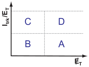
Figure 15: The arrangement of the four categories of events used in the ABCD method. The vertical scale indicates increasing values of relative track isolation $I_{\textrm{trk}}/\ET$ and the horizontal scale indicates increasing ${E\!\!\!/}_{\!\mathrm{T}}$.

Similarly, the regions above and below the ${E\!\!\!/}_{\!\mathrm{T}}$ boundary for $I_{\textrm{trk}}/\ET$ values above 0.04, but below an upper $I_{\textrm{trk}}/\ET$ bound of 0.2 (0.1) for electrons in the EB (EE), define the regions D and C, respectively. There is no upper bound for the ${E\!\!\!/}_{\!\mathrm{T}}$ values. The different regions are shown graphically in Fig. 15, with region A having the greatest signal purity. Combined regions are referred to as ’AB’ (for A and B), for example. The extracted signal corresponds to the entire ABCD region.

A system of equations is constructed relating the numbers of observed data events in each of the four regions to the numbers of background and signal events, with several parameters to be determined from auxiliary measurements or simulations. In this formulation, two parameters, $f_{\mathrm{A}}$ and $f_{\mathrm{D}}$, relate to the QCD backgrounds and are defined as the ratios of events with a fake electron candidate in the A and D regions to the number in the AB and CD regions, respectively. The two parameters represent the efficiency with which misidentified electrons pass the boundary on ${E\!\!\!/}_{\!\mathrm{T}}$ dividing AD from BC. If the efficiency for passing the ${E\!\!\!/}_{\!\mathrm{T}}$ boundary is largely independent of the choice of the boundaries on $I_{\textrm{trk}}/\ET$, then these two parameters will be approximately equal. Assuming $f_{\mathrm{A}}=f_{\mathrm{D}}$ holds exactly leads to a simplification of the system of equations such that all direct dependence of the signal extraction on parameters related to the QCD backgrounds is eliminated. For this idealized case there would be no uncertainty on the extracted signal yield arising from modeling of QCD backgrounds. Detailed studies of the data suggest this assumption holds to a good degree. A residual bias in the extracted signal arising from this assumption is estimated directly from the data by studying a control sample obtained with inverted quality requirements on the electron candidate, and an appropriate small correction to the yield is applied (${\approx}0.37\%$). A systematic uncertainty on the signal yield is derived from the uncertainty on this bias correction. This contribution is small and is dominated by the uncertainty on signal contamination in the control sample.

Three other important parameters relate to signal efficiencies: $\epsilon_{\mathrm{A}}$ and $\epsilon_{\mathrm{D}}$, which are the efficiencies for signal events in the AB and CD regions, respectively, to pass the ${E\!\!\!/}_{\!\mathrm{T}}$ boundary, and $\epsilon_{\mathrm{P}}$, which is the efficiency for the electron candidate of a signal event to pass the boundary on relative track isolation dividing the AB region from the CD region under the condition that this electron already lies in the ABCD region. The first two of these, $\epsilon_{\mathrm{A}}$ and $\epsilon_{\mathrm{D}}$, are estimated from models of the ${E\!\!\!/}_{\!\mathrm{T}}$ in signal events using the methods described in Section 0.7.1. The third parameter, $\epsilon_{\mathrm{P}}$, is measured from data using the T&P method, described in Section 0.6.1, and is one of the dominant sources of uncertainty on the $\mathrm{W}$ boson yield before considering the final acceptance corrections.

Electroweak background contributions are estimated from MC samples with an overall normalization scaled through an iterative method with the signal yield.

The extracted yield with respect to the choice of boundaries in relative track isolation and ${E\!\!\!/}_{\!\mathrm{T}}$ is sensitive to biases in $\epsilon_{\mathrm{P}}$ and the QCD electron misidentification rate bias correction described above, respectively. The yield is very stable with respect to small changes in these selections, giving confidence that these important sources of systematic uncertainty are small.

The following signal yields are obtained: $136\,003\pm 498\,\mathrm{(stat.)}$ for the inclusive sample, $81\,525\pm 385\,\mathrm{(stat.)}$ for the $\mathrm{W^{+}}\rightarrow\mathrm{e}^{+}\nu$ sample, and $54\,356\pm 315\,\mathrm{(stat.)}$ for the $\mathrm{W^{-}}\rightarrow\mathrm{e}^{-}\overline{\nu}$ sample. The ratios of the inclusive, $\mathrm{W^{+}}\rightarrow\mathrm{e}^{+}\nu$, and $\mathrm{W^{-}}\rightarrow\mathrm{e}^{-}\overline{\nu}$ yields between this method and the parameterized QCD shape are $0.998\pm 0.007$, $0.999\pm 0.007$, and $0.993\pm 0.007$, respectively, considering only the uncorrelated systematic uncertainties between the two methods.

The results of the three signal extraction methods are summarised in Table 8.

Table 8: Comparison of $\mathrm{W}\rightarrow\mathrm{e}\nu$ signal extraction methods. The signal yield of each method is presented together with its statistical uncertainty. For the fixed shape and the ABCD methods, the ratios of the signal yields with the analytical function method are also shown taking into account only the uncorrelated systematics between the methods used in the ratios.

Source		$\mathrm{W}\rightarrow\mathrm{e}\nu$	$\mathrm{W^{+}}\rightarrow\mathrm{e}^{+}\nu$	$\mathrm{W^{-}}\rightarrow\mathrm{e}^{-}\overline{\nu}$
Analytical fun.	yield	$136\,328\pm 386$	$81\,568\pm 297$	$54\,760\pm 246$
Fixed shape	yield	$135\,982\pm 388$	$81\,286\pm 302$	$54\,703\pm 249$
	ratio	$0.997\pm 0.005$	$0.997\pm 0.005$	$0.999\pm 0.005$
ABCD	yield	$136\,003\pm 498$	$81\,525\pm 385$	$54\,356\pm 315$
	ratio	$0.998\pm 0.007$	$0.999\pm 0.007$	$0.993\pm 0.007$

0.7.4 Modeling of the QCD Background and $\mathrm{W}\rightarrow\mu\nu$ Signal Yield

The $\mathrm{W}\rightarrow\mu\nu$ analysis is performed using fixed distributions for the ${E\!\!\!/}_{\!\mathrm{T}}$ shapes obtained from data for the QCD background component and from simulations, after applying proper corrections, for the signal and the remaining background components.

Different approaches to signal extraction are considered for $\mathrm{W}\rightarrow\mu\nu$, as for $\mathrm{W}\rightarrow\mathrm{e}\nu$. The alternative methods do not demonstrate better performance than the use of fixed shapes in the W signal fit. Given the lower backgrounds in the muon channel with respect to the electron channel, the alternative strategies are not pursued at the same level of detail as in the electron case.

The ${E\!\!\!/}_{\!\mathrm{T}}$ shape of the QCD background component is obtained from a high-purity QCD sample of events that pass the signal selection, except that the isolation requirement is inverted and set to $I^{\textrm{rel}}_{\textrm{comb}}>0.2$ (Fig. 4).

Simulation studies indicate that this distribution does not accurately reproduce the ${E\!\!\!/}_{\!\mathrm{T}}$ shape when muon isolation is required. This is shown in Fig. 16 (left), where the solid line represents the shape for events with an isolated muon and the dashed line the shape obtained by inverting the isolation requirement.

A positive correlation between the isolation variable $I^{\textrm{rel}}_{\textrm{comb}}$ and ${E\!\!\!/}_{\!\mathrm{T}}$ is shown in Fig. 16 (right, red open circles). This behavior can be parameterized in terms of a linear function ${E\!\!\!/}_{\!\mathrm{T}}\propto(1+\alpha\,I^{\textrm{rel}}_{\textrm{comb}})$, as shown in the same figure. A compensation for the correlation is subsequently made by applying a correction of the kind of ${E\!\!\!/}_{\!\mathrm{T}}^{\prime}={E\!\!\!/}_{\!\mathrm{T}}/(1+\alpha\,I^{\textrm{rel}}_{\textrm{comb}})$ to the events selected by inverting the isolation requirement and a new corrected shape is obtained. The agreement of this new shape (black points in Fig. 16, left) with the prediction from events with an isolated muon is considerably improved. It is also observed that a maximal variation in the correction factor of $\Delta\alpha=0.08$ successfully covers the simulation prediction for events with an isolated muon over the whole ${E\!\!\!/}_{\!\mathrm{T}}$ interval (shaded area in Fig. 16, left).

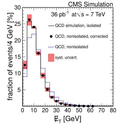
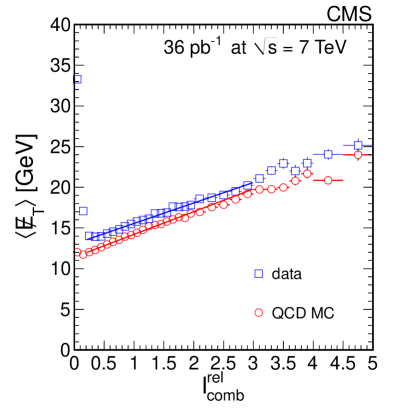
Figure 16: Left: distribution of the corrected ${E\!\!\!/}_{\!\mathrm{T}}$ for selected events with a non isolated muon (black points) superimposed on the distribution of uncorrected ${E\!\!\!/}_{\!\mathrm{T}}$ for the same events (blue, dashed line) and ${E\!\!\!/}_{\!\mathrm{T}}$ for events with an isolated muon (black, solid histogram). All distributions are from simulated QCD events. The shaded area represents the systematic uncertainty due to corrections with factors $\alpha\pm\Delta\alpha$, for $\Delta\alpha=0.08$. Right: distribution of the average ${E\!\!\!/}_{\!\mathrm{T}}$ versus $I^{\textrm{rel}}_{\textrm{comb}}$ for simulated QCD events (red circles) and for data (blue squares). The high values of ${E\!\!\!/}_{\!\mathrm{T}}$ in the first two bins in $I^{\textrm{rel}}_{\textrm{comb}}$ are due to the presence of the W signal events. The superimposed lines are linear fits in the range $[0.2,3.0]$ of $I^{\textrm{rel}}_{\textrm{comb}}$.

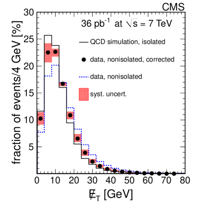
Figure 17: Distribution of the corrected ${E\!\!\!/}_{\!\mathrm{T}}$ for selected events with a nonisolated muon in data (black points) superimposed on the uncorrected ${E\!\!\!/}_{\!\mathrm{T}}$ distributions for data (blue dashed line) and simulated QCD events (black, solid histogram, same as the black, solid histogram in Fig. 16). The shaded area represents the systematic uncertainty due to corrections with factors $\alpha\pm\Delta\alpha$ for $\Delta\alpha=0.08$.

The same positive correlation between ${E\!\!\!/}_{\!\mathrm{T}}$ and $I^{\textrm{rel}}_{\textrm{comb}}$ is observed in the data (blue squares in Fig. 16, right). A correction ${E\!\!\!/}_{\!\mathrm{T}}^{\prime}={E\!\!\!/}_{\!\mathrm{T}}/(1+\alpha\,I^{\textrm{rel}}_{\textrm{comb}})$, with $\alpha\approx 0.2$, was applied. The shapes obtained in data are shown in Fig. 17 where the uncorrected and corrected data shapes from events selected by inverting the isolation requirement, together with the simulation expectation for events with an isolated muon, are shown. The shaded area in Fig. 17 is bounded by the two distributions, obtained using two extreme correction parameters $\alpha\pm\Delta\alpha$, with $\Delta\alpha=0.08$, as evaluated in simulations. This area is taken as a systematic uncertainty on the QCD background shape.

Several parameterizations for the correction are considered, but the impact on the corrected distribution and therefore on the final result is small. Associated uncertainties on the cross section and ratios are evaluated as the differences between the fit results obtained with the optimal $\alpha$ value and two extreme cases, $\alpha\pm\Delta\alpha$.

The following signal yields are obtained: $140\,757\pm 383$ for the inclusive sample, $56\,666\pm 240$ for the $\mathrm{W^{-}}\rightarrow\mu^{-}\overline{\nu}$ sample, and $84\,091\pm 291$ for the $\mathrm{W^{+}}\rightarrow\mu^{+}\nu$ sample.

The ${E\!\!\!/}_{\!\mathrm{T}}$ distributions are presented in Fig. 18 (full sample) and Fig. 19 (samples selected by the muon charge) superimposed on the individual fitted contributions of the W signal and the EWK and QCD backgrounds. Figures 18 and 19 show the ${E\!\!\!/}_{\!\mathrm{T}}$ distributions for data and fitted signal, plus background components. Figure 20 shows the $M_{\mathrm{T}}$ distributions for data and signal, plus background components, fitted from the ${E\!\!\!/}_{\!\mathrm{T}}$ spectra.

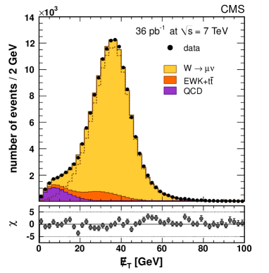
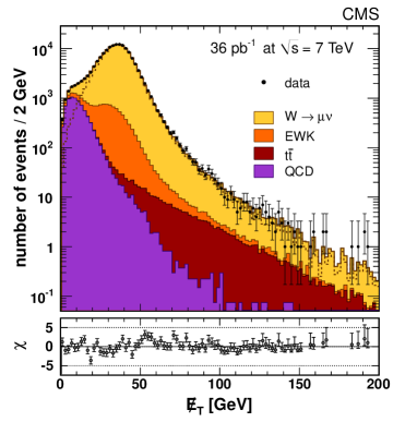
Figure 18: The ${E\!\!\!/}_{\!\mathrm{T}}$ distribution for the selected $\mathrm{W}\rightarrow\mu\nu$ candidates on a linear scale (left) and on a logarithmic scale (right). The points with the error bars represent the data. Superimposed are the contributions obtained with the fit for QCD background (violet, dark histogram), all other backgrounds (orange, medium histogram), and signal plus background (yellow, light histogram). The black dashed line is the fitted signal contribution.

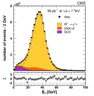
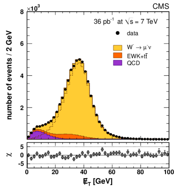
Figure 19: The ${E\!\!\!/}_{\!\mathrm{T}}$ distributions for the selected W⁺ (left) and W^- (right) candidates. The points with the error bars represent the data. Superimposed are the contributions obtained with the fit for QCD background (violet, dark histogram), all other backgrounds (orange, medium histogram), and signal plus background (yellow, light histogram). The black dashed line is the fitted signal contribution.

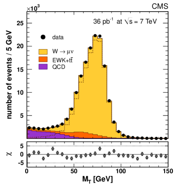
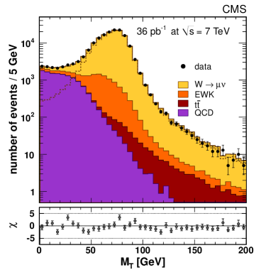
Figure 20: The $M_{\mathrm{T}}$ distribution for the selected $\mathrm{W}\rightarrow\mu\nu$ candidates on a linear scale (left) and on a logarithmic scale (right). The points with the error bars represent the data. Superimposed are the contributions obtained with the fit for QCD background (violet, dark histogram), all other backgrounds (orange, medium histogram), and signal plus background (yellow, light histogram). The black dashed line is the fitted signal contribution.

0.8 The $\mathrm{Z}\rightarrow\ell^{+}\ell^{-}$ Signal Extraction

The $\mathrm{Z}\rightarrow\ell^{+}\ell^{-}$ yield can be obtained by counting the number of selected candidates after subtracting the residual background. The $\mathrm{Z}\rightarrow\ell^{+}\ell^{-}$ yield and lepton efficiencies are also determined using a simultaneous fit to the invariant mass spectra of multiple dilepton categories. The simultaneous fit deals correctly with correlations in determining the lepton efficiencies and the $\mathrm{Z}$ yield from the same sample. The Z yield extracted in this way does not need to be corrected for efficiency effects in order to determine the cross section, and the statistical uncertainty on the $\mathrm{Z}$ yield absorbs the uncertainties on the determination of lepton efficiencies that would be propagated as systematic uncertainties in the counting analysis. Both methods were performed for the $\mathrm{Z}\rightarrow\mathrm{e}^{+}\mathrm{e}^{-}$ analysis, while only the simultaneous fit was used for the $\mathrm{Z}\rightarrow\MM$ analysis after taking into account the results from the previous studies [21].

0.8.1 EWK and QCD Backgrounds

For the $\mathrm{Z}\rightarrow\mathrm{e}^{+}\mathrm{e}^{-}$ analysis the background contributions from EWK processes $\mathrm{Z}\rightarrow\tau^{+}\tau^{-}$, $\mathrm{t}\bar{\mathrm{t}}$, and diboson production are estimated from the yields of events selected in NLO MC samples normalized to the NNLO cross sections and scaled to the considered integrated luminosity. They amount to $30.8\pm 0.4$ events, where the uncertainty combines the NNLO and luminosity uncertainties. Data are used to estimate the background originating from W+jets, $\gamma$+jets, and QCD multijet events where the selected electrons come from misidentified jets or photons (referred to as ’QCD background’). This background contribution is estimated using the distribution of the relative track isolation, $I_{\textrm{trk}}/E\,\,_{\!\!\!\mathrm{T}}$, and amounts to $4.9\pm 8.4\,\textrm{(stat.)}\pm 8.4\,\textrm{(syst.)}$ events. As a cross-check, the “same-sign/opposite-sign” method was used, which is based on the signs of the charges of the two electron candidates, the measured charge misidentification for electrons that pass the nominal selection criteria, and the hypothesis that the QCD background is charge-symmetric. The QCD background estimate with this method is $59\pm 17\textrm{(stat.)}\pm 160\,\textrm{(syst.)}$ events. The two methods are consistent with the presence of negligible QCD background in our sample.

Backgrounds in the $\mathrm{Z}\rightarrow\MM$ analysis containing two isolated global muons have been estimated with simulations to be very small. This category of dimuon events is defined as the “golden” category. The simulation prediction of the smallness of the $\mathrm{t}\bar{\mathrm{t}}$ and QCD backgrounds was validated with data. First, the selected dimuon sample was enriched with $\mathrm{t}\bar{\mathrm{t}}$ events by applying a requirement on ${E\!\!\!/}_{\!\mathrm{T}}$, because of the presence of neutrinos in $\mathrm{t}\bar{\mathrm{t}}$ events, and an agreement between data and the simulation prediction was found with the dimuon invariant mass requirement inverted, where the residual Z signal is negligible. The QCD component has been checked using the same-sign dimuon events and dimuon events with both muons failing the isolation requirement, and was found to be in agreement with the simulation predictions. The conclusion from the maximum amount of measured data-simulation discrepancy was that the uncertainty in the residual background subtraction has a negligible effect on the $\mathrm{Z}\rightarrow\MM$ measured yield. The backgrounds to the $\mathrm{Z}\rightarrow\MM$ categories having one global and one looser muon are significantly larger than in the golden category. Simulation estimates in this case are not used for such backgrounds and fits to the dimuon invariant mass distributions are performed including parameterized background components, as described in Section 0.8.3.

Backgrounds estimates in the $\mathrm{Z}\rightarrow\mathrm{e}^{+}\mathrm{e}^{-}$ and $\mathrm{Z}\rightarrow\MM$ analyses are summarized in Table 9.

Table 9: Estimated background-to-signal ratios in the $\mathrm{Z}\rightarrow\mathrm{e}^{+}\mathrm{e}^{-}$ and $\mathrm{Z}\rightarrow\MM$ (only for candidates in the golden category) channels. The QCD background for the $\mathrm{Z}\rightarrow\mathrm{e}^{+}\mathrm{e}^{-}$ channel has been estimated with data, while all other estimates are based on MC simulations, and their corresponding uncertainties are statistical only.

Processes	$\mathrm{Z}\rightarrow\mathrm{e}^{+}\mathrm{e}^{-}$ sel.	$\mathrm{Z}\rightarrow\MM$ sel.
Diboson production	$(0.157\pm 0.001)\%$	$(0.158\pm 0.001)\%$
$\mathrm{t}\bar{\mathrm{t}}$	$(0.117\pm 0.008)\%$	$(0.141\pm 0.014)\%$
$\mathrm{Z}\rightarrow\tau^{+}\tau^{-}$	$(0.080\pm 0.006)\%$	$(0.124\pm 0.005)\%$
W+jets	$(0.010\pm 0.002)\%$	$(0.008\pm 0.002)\%$
Total EWK plus $\mathrm{t}\bar{\mathrm{t}}$	$(0.365\pm 0.010)\%$	$(0.430\pm 0.015)\%$
QCD	$(0.06\pm 0.14)\%$	$(0.013\pm 0.001)\%$
Total background	$(0.42\pm 0.14)\%$	$(0.444\pm 0.015)\%$

0.8.2 The $\mathrm{Z}\rightarrow\mathrm{e}^{+}\mathrm{e}^{-}$ Signal Extraction

In the following sections the use of a pure $\mathrm{Z}\rightarrow\mathrm{e}^{+}\mathrm{e}^{-}$ sample for the determination of the residual energy-scale and resolution corrections is first discussed. Then the signal extraction with the counting analysis and the simultaneous fit methods are presented.

Electron Energy Scale

The lead tungstate crystals of the ECAL are subject to transparency loss during irradiation, followed by recovery in periods with no irradiation. The magnitude of the changes to the energy response is dependent on instantaneous luminosity and was, at the end of the 2010 data taking period, up to 1$\%$ in the barrel region, and 4$\%$ or more in parts of the endcap. The changes are monitored continuously by injecting laser light and recording the response. The corrections derived from this monitoring are validated by studying the variation of the $\pi^{0}$ mass peak as a function of time for different regions of the ECAL (using $\pi^{0}$ data collected in a special calibration stream), and by studying the overall $\mathrm{Z}\rightarrow\mathrm{e}^{+}\mathrm{e}^{-}$ mass peak and width. With the current corrections, residual variations of the energy scale with time are at the level of 0.3% in the barrel and less than 1% in the endcaps.

The remaining mean scale correction factors to be applied to the data and the resolution corrections (smearing) to be applied to the simulated sample are estimated from $\mathrm{Z}\rightarrow\mathrm{e}^{+}\mathrm{e}^{-}$ events. Invariant mass distributions for electrons in several $\eta$ bins in the EB and EE are derived from simulations and compared to data. A simultaneous fit of a Breit–Wigner convolved with a Crystal-Ball function to each $\mathrm{Z}\rightarrow\mathrm{e}^{+}\mathrm{e}^{-}$ mass distribution is performed in order to determine the energy scale correction factors for the data and the resolution smearing corrections for the simulated samples. The energy scale correction factors are below 1$\%$ while the resolution smearing corrections are below 1$\%$ everywhere, with the exception of the transition region between the EB and the EE, where they reach 2$\%$. Those corrections are propagated in the analysis and proper systematic uncertainties for the cross section measurements are estimated as discussed in Section 0.9.1.

Counting Analysis

After energy scale corrections, applied to electron ECAL clusters before any threshold requirement, 10 fewer events ($-0.12\%$) were selected compared to the number of selected events before the application of the energy scale corrections. This brings the final $\mathrm{Z}\rightarrow\mathrm{e}^{+}\mathrm{e}^{-}$ sample to $8442$ and, after background subtraction, the $\mathrm{Z}$ yield is $8406\pm 92$ events. This yield is used for the cross section estimation.

The dielectron invariant mass spectra for the selected sample with the tight selection before and after the application of the corrections are shown in Fig. 21 along with the predicted distributions. The data and simulation distributions are normalized to account for the difference in selection efficiency.

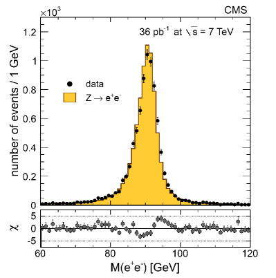
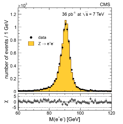
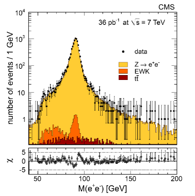
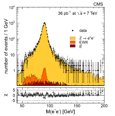
Figure 21: Distributions of the dielectron invariant mass for the selected $\mathrm{Z}\rightarrow\mathrm{e}^{+}\mathrm{e}^{-}$ candidates on a linear scale (top) and on a logarithmic scale (bottom) before (left) and after (right) applying energy-scale correction factors. The points with the error bars represent the data. Superimposed are the expected distributions from simulations, normalized to an integrated luminosity of $36$ pb^-1. The expected distributions are the Z signal (yellow, light histogram), other EWK processes (orange, medium histogram), and $\mathrm{t}\bar{\mathrm{t}}$ background (red, dark histogram). Backgrounds are negligible and cannot be seen on the linear-scale plots.

Simultaneous Fit

The $\mathrm{Z}$ event yield and the electron efficiencies can be extracted from a simultaneous fit. Two categories of events are considered: events where both electrons satisfy the tight selection with $E\,\,_{\!\!\!\mathrm{T}}>25\GeV$, and events that consist of one electron with $E\,\,_{\!\!\!\mathrm{T}}>25\GeV$ that passes the tight selection, and one ECAL cluster with $E\,\,_{\!\!\!\mathrm{T}}>25\GeV$ that fails the selection, either at the reconstruction or electron identification level.

In each category, a signal-plus-background function is fitted to the observed mass spectrum. The signal shape is taken from signal samples simulated with POWHEG at the NLO generator level, and is convolved with a Crystal-Ball function modified to include an extra Gaussian on the high end tail with floating mean and width. In the first category, the nearly vanishing background is fixed to the value reported in Table 9. In the second category of events, the background is modeled by an exponential distribution.

The estimated cross section is $988\pm 10\,\mathrm{(stat.)}\pm 4\mathrm{(syst.)}\,\mathrm{pb}$. The cross section is in good agreement with the counting analysis estimate of $992\pm 11\,\mathrm{(stat.)}\,\mathrm{pb}$, considering only the statistical uncertainty. Both techniques give equivalent results. The counting analysis estimate is used for the cross section measurement in the $\mathrm{Z}\rightarrow\mathrm{e}^{+}\mathrm{e}^{-}$ channel.

0.8.3 The $\mathrm{Z}\rightarrow\MM$ Signal Extraction

The yield of the $\mathrm{Z}\rightarrow\MM$ events is determined from a fit simultaneously with the average muon reconstruction efficiencies in the tracker and in the muon detector, the muon trigger efficiency, as well as the efficiency of the applied isolation requirement. $\mathrm{Z}\rightarrow\MM$candidates are obtained as pairs of muon candidates of different types and organized into categories according to different requirements:

• $\mathrm{Z}_{\mu\mu}$: a pair of isolated global muons, further split into two samples:

  • $\mathrm{Z}_{\mu\mu}^{2\mathrm{HLT}}$: each muons associated with an HLT trigger muon;

  • $\mathrm{Z}_{\mu\mu}^{1\mathrm{HLT}}$: only one of the two muons associated with an HLT trigger muon;

• $\mathrm{Z}_{\mu s}$: one isolated global muon and one isolated stand-alone muon;

• $\mathrm{Z}_{\mu t}$: one isolated global muon and one isolated tracker track;

• $\mathrm{Z}_{\mu\mu}^{\mathrm{noniso}}$: a pair of global muons, of which one is isolated and the other is nonisolated.

With the exception of the $\mathrm{Z}_{\mu\mu}^{1\mathrm{HLT}}$ category, each global muon must correspond to an HLT trigger muon. The five categories are explicitly forced to be mutually exclusive in the event selection: if one event falls into the first category it is excluded from the second; if it does not fall into the first category and falls into the second, it is excluded from the third, and so on. In this way non-overlapping, hence statistically independent, event samples are defined. The expected number of events in which more than one dimuon combination is selected is almost negligible. In those few cases all possible combinations are considered.

The five unknowns, the Z yield and four efficiency terms, can be written in terms of the five signal yields in each category as follows:

$$N_{\mu\mu}^{2\mathrm{HLT}} = N_{\mathrm{Z}\rightarrow\MM}\epsilon_{\mathrm{HLT}}^{2}\epsilon_{\mathrm{iso}}^{2}\epsilon_{\mathrm{trk}}^{2}\epsilon_{\mathrm{sa}}^{2},$$ (4)

$$N_{\mu\mu}^{1\mathrm{HLT}} = 2N_{\mathrm{Z}\rightarrow\MM}\epsilon_{\mathrm{HLT}}(1-\epsilon_{\mathrm{HLT}})\epsilon_{\mathrm{iso}}^{2}\epsilon_{\mathrm{trk}}^{2}\epsilon_{\mathrm{sa}}^{2},$$ (5)

$$N_{\mu s} = 2N_{\mathrm{Z}\rightarrow\MM}\epsilon_{\mathrm{HLT}}\epsilon_{\mathrm{iso}}^{2}\epsilon_{\mathrm{trk}}(1-\epsilon_{\mathrm{trk}})\epsilon_{\mathrm{sa}}^{2},$$ (6)

$$N_{\mu t} = 2N_{\mathrm{Z}\rightarrow\MM}\epsilon_{\mathrm{HLT}}\epsilon_{\mathrm{iso}}^{2}\epsilon_{\mathrm{trk}}^{2}\epsilon_{\mathrm{sa}}(1-\epsilon_{\mathrm{sa}}),$$ (7)

$$N_{\mu\mu}^{\mathrm{noniso}} = 2N_{\mathrm{Z}\rightarrow\MM}\epsilon_{\mathrm{HLT}}^{2}\epsilon_{\mathrm{iso}}(1-\epsilon_{\mathrm{iso}})\epsilon_{\mathrm{trk}}^{2}\epsilon_{\mathrm{sa}}^{2}.$$ (8)

The various efficiency terms in Eqs. (4) to (8), the average efficiencies of muon reconstruction in the tracker, $\epsilon_{\mathrm{trk}}$, in the muon detector as a stand-alone muon, $\epsilon_{\mathrm{sa}}$, the average efficiency of the isolation requirement, $\epsilon_{\mathrm{iso}}$, and the average trigger efficiency, $\epsilon_{\mathrm{HLT}}$, can be factorized because the muon selection factorizes the requirements on the tracker and muon detector quantities separately. Neither selection on $\chi^{2}$ per degree of freedom nor requirement of the muon reconstruction through the tracker-muon algorithm is applied in order to avoid efficiency terms that cannot be described as a product of contributions from the tracker and the muon detector.

The dimuon invariant mass spectra for the five categories are divided into bins of different sizes, depending on the number of observed events. The distributions of the dimuon invariant mass for the different categories can be written as the sum of a signal peak plus a background component.

Figure 22 shows the dimuon invariant mass spectrum for the $\mathrm{Z}\rightarrow\MM$ golden events on both a linear scale and a logarithmic scale, and Figs. 23 and 24 show the invariant mass distributions for the remaining categories. The spectra are in agreement with the simulation.

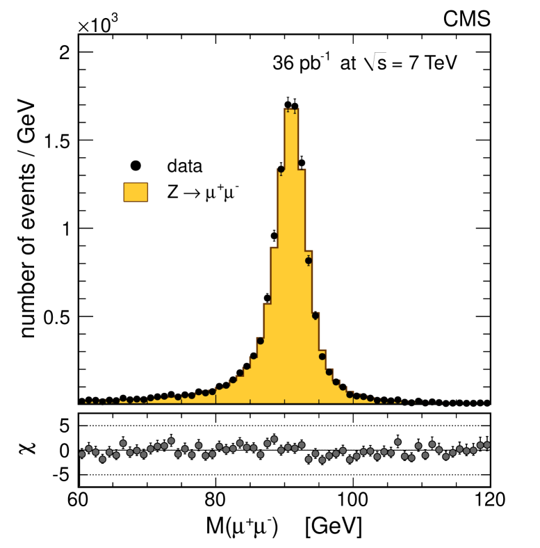
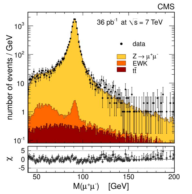
Figure 22: Distributions of the dimuon invariant mass for the selected $\mathrm{Z}\rightarrow\MM$ golden candidates on a linear scale (left) and on a logarithmic scale (right). The points with the error bars represent the data. Superimposed are the expected distributions from simulations, normalized to an integrated luminosity of $36$ pb^-1. The expected distributions are the Z signal (yellow, light histogram), other EWK processes (orange, medium histogram), and $\mathrm{t}\bar{\mathrm{t}}$ background (red, dark histogram). Backgrounds are negligible and cannot be seen on the linear-scale plots.

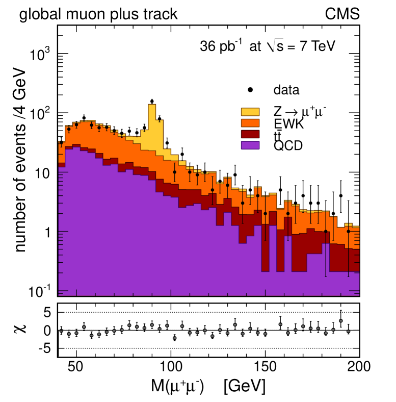
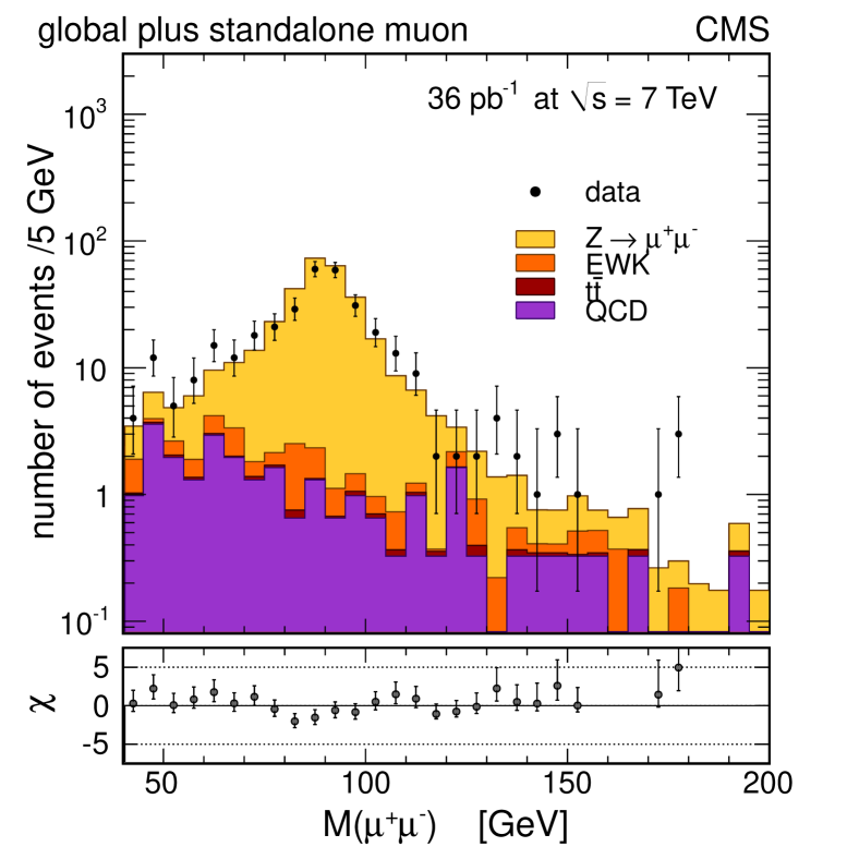
Figure 23: Distributions of the dimuon invariant mass for the selected $\mathrm{Z}_{\mu t}$ (left) and $\mathrm{Z}_{\mu s}$ (right) candidates. The points with the error bars represent the data. Superimposed are the expected distributions from simulations, normalized to an integrated luminosity of $36$ pb^-1. The expected distributions are the Z signal (yellow, light histogram), other EWK processes (orange, medium histogram), $\mathrm{t}\bar{\mathrm{t}}$ background (red, dark histogram) and QCD background (violet, black histogram).

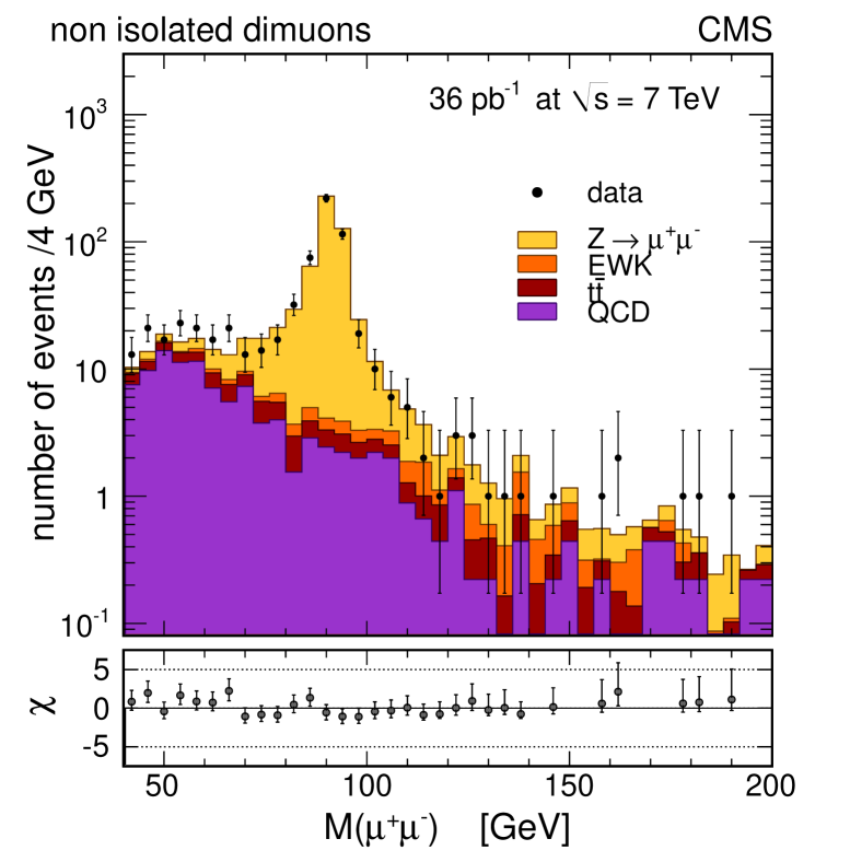
Figure 24: Distributions of the dimuon invariant mass for the selected $\mathrm{Z}_{\mu\mu}^{\mathrm{noniso}}$ candidates. The points with the error bars represent the data. Superimposed are the expected distributions from simulations, normalized to an integrated luminosity of $36$ pb^-1. The expected distributions are the Z signal (yellow, light histogram), other EWK processes (orange, medium histogram), $\mathrm{t}\bar{\mathrm{t}}$ background (red, dark histogram), and QCD background (violet, black histogram).

The signal-peak distribution can be considered to be identical in the categories $\mathrm{Z}_{\mu\mu}$ and $\mathrm{Z}_{\mu t}$ because the momentum resolution in CMS is determined predominantly by the tracker measurement for muons with $p_{\mathrm{T}}\leq 200$ GeV. The binned spectrum of the dimuon invariant mass in the $\mathrm{Z}_{\mu\mu}$ category, which has the most events of all categories, is taken as shape model for all categories but $\mathrm{Z}_{\mu s}$. The large size of the golden sample ensures that the statistical uncertainty of the invariant mass distribution has a negligible effect on the cross section measurement. The small presence of background is neglected in this distribution. The uncertainty due to this approximation has been evaluated and taken as the systematic uncertainty as described in Section 0.9.2.

Because only tracker isolation is used, the shape obtained from golden events can also be used to model the $\mathrm{Z}_{\mu\mu}^{\mathrm{noniso}}$ peak distribution. A requirement on calorimetric isolation would have distorted the dimuon invariant mass distribution of events with one nonisolated muon because of FSR, as has been observed both in simulation and data.

The model of the invariant mass shape for the $\mathrm{Z}_{\mu s}$ category is also derived from golden dimuon events. The three-momentum for one of the two muons is taken from only the muon detector track fit, in order to emulate a stand-alone muon. To avoid using the same event twice in forming the $\mathrm{Z}_{\mu s}$ shape model, the higher-$p_{\mathrm{T}}$ (lower-$p_{\mathrm{T}}$) muon is chosen for even (odd) event numbers.

Background shapes are modeled as products of an exponential times a polynomial whose degree depends on the category. Different background models and different binning sizes are considered for the categories other than $\mathrm{Z}_{\mu\mu}$ and a systematic uncertainty related to the fitting procedure is determined accordingly.

A simultaneous binned fit based on a Poissonian likelihood [43] is performed for the different categories. Table 10 reports the signal yield and single-muon efficiencies determined from the simultaneous fit and the ratios of the fitted to simulation efficiencies. A goodness-of-fit test gives a probability ($p$-value) of 0.36 for this fit.

Table 10: Signal yield and efficiencies determined from data with the simultaneous fit, and ratios of efficiencies determined from the fit and the simulation.

Quantity	Fit results from data	Data/simulation
$N_{\mathrm{Z}\rightarrow\MM}$	13 728 $\pm$ 121
$\epsilon_{\mathrm{HLT}}$	0.9203 $\pm$ 0.0019	0.9672 $\pm$ 0.0020
$\epsilon_{\mathrm{iso}}$	0.9813 $\pm$ 0.0010	0.9962 $\pm$ 0.0011
$\epsilon_{\mathrm{sa}}$	0.9762 $\pm$ 0.0012	0.9964 $\pm$ 0.0013
$\epsilon_{\mathrm{trk}}$	0.9890 $\pm$ 0.0006	0.9949 $\pm$ 0.0007

The background in the $\mathrm{Z}_{\mu\mu}$ golden category (of the order of few per mille) was neglected in the fit. In order to correct the fitted yield $N_{\mathrm{Z}\rightarrow\MM}$ for the presence of this background, we subtract the small estimated irreducible background fraction.

A $(1.0\pm 0.5)\%$ overall efficiency correction due to the loss of muon events because of trigger prefiring is also applied (Section 0.6.2).

The estimated cross section is $968\pm 8\mathrm{(stat.)}$ pb.

0.9 Systematic Uncertainties

The largest uncertainty contribution on the measured cross sections is related to the integrated luminosity [44], and amounts to $4\%$.

The next most important source of systematic uncertainty is due to the lepton efficiency correction factors obtained from the T&P method. In the $\mathrm{Z}\rightarrow\MM$ analysis, the efficiency uncertainties are absorbed in the statistical uncertainty of the measurement, via the simultaneous fit to the yield and efficiencies.

Table 11 shows a summary of systematic uncertainties for the $\mathrm{W}$ and $\mathrm{Z}$ cross section measurements. Tables 12 and 13 show a summary of systematic uncertainties for the individual cross sections ($\mathrm{W^{+}},\mathrm{W^{-}}$) and the ratios ($\mathrm{W^{+}}/\mathrm{W^{-}}$, $\mathrm{W}/\mathrm{Z}$). Details of systematic uncertainties for the muon and electron channels are described in the following subsections.

Table 11: Systematic uncertainties in percent for inclusive W and Z cross sections. The “n/a” entry means that the source does not apply. A common luminosity uncertainty of 4% applies to all channels.

Source	$\mathrm{W}\rightarrow\mathrm{e}\nu$	$\mathrm{W}\rightarrow\mu\nu$	$\mathrm{Z}\rightarrow\mathrm{e}^{+}\mathrm{e}^{-}$	$\mathrm{Z}\rightarrow\MM$
Lepton reconstruction & identification	$1.4$	$0.9$	$1.8$	n/a
Trigger prefiring	n/a	$0.5$	n/a	$0.5$
Energy/momentum scale & resolution	$0.5$	$0.22$	$0.12$	$0.35$
${E\!\!\!/}_{\!\mathrm{T}}$ scale & resolution	$0.3$	$0.2$	n/a	n/a
Background subtraction / modeling	$0.35$	$0.4$	$0.14$	$0.28$
Trigger changes throughout 2010	n/a	n/a	n/a	$0.1$
Total experimental	$1.6$	$1.1$	$1.8$	$0.7$
PDF uncertainty for acceptance	$0.6$	$0.8$	$0.9$	$1.1$
Other theoretical uncertainties	$0.7$	$0.8$	$1.4$	$1.6$
Total theoretical	$0.9$	$1.1$	$1.6$	$1.9$
Total (excluding luminosity)	$1.8$	$1.6$	$2.4$	$2.0$

Table 12: Systematic uncertainties in percent for individual W cross sections and the ratios in the electron channel. A common luminosity uncertainty of 4% applies to all cross sections.

Source	$\mathrm{W^{+}}$ (e)	$\mathrm{W^{-}}$ (e)	$\mathrm{W^{+}}/\mathrm{W^{-}}$ (e)	$W/Z$ (e)
Lepton reconstruction & identification	1.5	1.5	1.5	1.1
Energy scale & resolution	0.5	0.6	0.1	0.2
${E\!\!\!/}_{\!\mathrm{T}}$ scale & resolution	0.3	0.3	0.1	0.3
Background subtraction / modeling	0.3	0.5	0.4	0.3
Total experimental	1.6	1.7	1.6	1.2
PDF uncertainty for acceptance	0.7	1.2	1.6	0.6
Other theoretical uncertainties	1.0	0.7	1.2	1.2
Total theoretical	1.2	1.4	2.0	1.4
Total (excluding luminosity)	2.1	2.2	2.6	1.8

Table 13: Systematic uncertainties in percent for individual W cross sections and ratios in the muon channel. A common luminosity uncertainty of 4% applies to all cross sections.

Source	$\mathrm{W^{+}}$ ($\mu$)	$\mathrm{W^{-}}$ ($\mu$)	$\mathrm{W^{+}}/\mathrm{W^{-}}$ ($\mu$)	$W/Z$ ($\mu$)
Lepton reconstruction & identification	0.9	0.9	1.3	0.9
Trigger prefiring	0.5	0.5	0	0
Momentum scale & resolution	0.19	0.25	0.06	0.35
${E\!\!\!/}_{\!\mathrm{T}}$ scale & resolution	0.2	0.2	0.0	0.2
Background subtraction / modeling	0.4	0.5	0.2	0.4
Total experimental	1.1	1.2	1.3	1.1
PDF uncertainty for acceptance	0.9	1.5	1.9	0.9
Other theoretical uncertainties	0.9	0.8	0.8	1.4
Total theoretical	1.3	1.7	2.1	1.6
Total (excluding luminosity)	1.7	2.1	2.5	2.0

0.9.1 Electron Channels

The propagation of statistical and systematic uncertainties on the data/simulation efficiency correction factors ($\rho$) from the T&P method (reconstruction, identification, and trigger) results in uncertainties of $1.4\%$ and $1.8\%$ for the $\mathrm{W}\rightarrow\mathrm{e}\nu$ and $\mathrm{Z}\rightarrow\mathrm{e}^{+}\mathrm{e}^{-}$ analyses, respectively. The uncertainties on the $\mathrm{W^{+}}$ and $\mathrm{W^{-}}$ cross sections are larger than that for the inclusive $\mathrm{W}$ because of the larger statistical uncertainty when efficiencies are estimated per charge. The systematic uncertainty, which depends on the efficiency under study, is determined by considering alternative signal and background models. The size of the systematic uncertainty is 0.3$\%$ for the electron selection efficiencies and 1.0$\%$ for the electron reconstruction efficiency. The estimation of the trigger efficiency is considered to be background-free so there is no need to perform a fit for the signal estimation. Theoretical uncertainties on the corrected efficiencies related to the PDF uncertainties and the PDF choice were found to be negligible.

The electron energy scale has an impact on the distribution for the signal. To study this effect, the energy-scale corrections obtained from the shift of the $\mathrm{Z}$ mass peak (Section 0.8.2) are applied to electrons in the EB and EE in simulation (before the $E\,\,_{\!\!\!\mathrm{T}}$ requirement) and the missing $E\,\,_{\!\!\!\mathrm{T}}$ is recomputed. The obtained variations on the signal yield from the UML fit are $0.5\%$ for the inclusive $\mathrm{W}$, $0.5\%$ for the $\mathrm{W^{+}}$, and $0.6\%$ for the $\mathrm{W^{-}}$ samples and $0.1\%$ on the $\mathrm{W^{+}}/\mathrm{W^{-}}$ ratio. All the charge-related studies (determination of individual $\mathrm{W^{+}}$ and $\mathrm{W^{-}}$ yields and $\mathrm{W^{+}}/\mathrm{W^{-}}$ ratio and associated systematic uncertainties) include data/simulation charge misidentification scale factors, estimated from the fraction of same-sign events in the $\mathrm{Z}\rightarrow\mathrm{e}^{+}\mathrm{e}^{-}$ data and simulated samples.

The energy scale of electrons has an impact on the $\mathrm{Z}$ yield because of the $E\,\,_{\!\!\!\mathrm{T}}>25~{}\GeV$ requirement on the two electrons and the mass window requirement. Applying the energy-scale corrections mentioned above to the EB and EE electrons and reprocessing the data, the $\mathrm{Z}$ yield is decreased by 10 events ($8452\to 8442$). A systematic uncertainty equal to this decrease of $0.12\%$ is assigned to the $\mathrm{Z}$ signal yield. The energy-scale uncertainty for the $\mathrm{W}$ selection is included in the systematic uncertainty described in the previous paragraph. There, the systematic uncertainty is larger than that for the $\mathrm{Z}$ selection because the energy scale also affects the ${E\!\!\!/}_{\!\mathrm{T}}$ shape used for the signal extraction. The $\mathrm{W}$ selection itself is affected by the energy scale at the level of $0.12\%$.

The ${E\!\!\!/}_{\!\mathrm{T}}$ shape used in the $\mathrm{W}$ fits is also distorted by energy resolution uncertainties; this induces a change in the $\mathrm{W}$ signal yield by 0.02%.

The ${E\!\!\!/}_{\!\mathrm{T}}$ energy scale is affected by our limited knowledge of the intrinsic hadronic recoil response. From the discrepancies found in the data/simulation comparisons (Section 0.7.1), uncertainties due to the ${E\!\!\!/}_{\!\mathrm{T}}$ energy scale are estimated to be 0.3% for inclusive $\mathrm{W}$, $\mathrm{W^{+}}$, and $\mathrm{W^{-}}$ yields, and 0.1% for the $\mathrm{W^{+}}/\mathrm{W^{-}}$ ratio.

The systematic uncertainties on the background subtraction address the possible difference between the true background distribution and the modified Rayleigh function that is used in the UML fit. We make the assumption that any such difference can be accounted for by an additional $\sigma_{2}$ parameter (defined in Section 0.7.3), which affects the resolution at large values of ${E\!\!\!/}_{\!\mathrm{T}}$ (below the signal). The value of $\sigma_{2}$ is first determined for three samples: the control sample in the data, the control sample in the QCD simulation, and the selected sample in the QCD simulation. The values obtained are $\sigma_{2}=0.0009~{}\GeV^{-1}$, $0.0010~{}\GeV^{-1}$, and $0.0007~{}\GeV^{-1}$, respectively for $\mathrm{W^{+}}$ and $\sigma_{2}=0.0007~{}\GeV^{-1}$, $0.0009~{}\GeV^{-1}$, and $0.0008~{}\GeV^{-1}$ for $\mathrm{W^{-}}$. The three values of $\sigma_{2}$ are then fixed in turn, and $\sigma_{0}$ and $\sigma_{1}$ are set to their values from data to generate distributions (of the size of our sample) with the three-parameter function, which we then fit with our nominal two-parameter function. The maximal relative difference in the yields is quoted as the systematic uncertainty on background subtraction: $0.35\%$ for inclusive $\mathrm{W}$, $0.33\%$ for $\mathrm{W^{+}}$, $0.48\%$ for $\mathrm{W^{-}}$, and $0.39\%$ for the ratio.

In the following paragraphs we discuss the systematic uncertainties of the fixed shape and the ABCD methods which were also explored in order to cross check the extraction of the $\mathrm{W}\rightarrow\mathrm{e}\nu$ signal. These uncertainties correspond to the specific methods and are not propagated to the final cross section measurement reported in this paper.

The systematic uncertainties on the background subtraction using fixed-shape distributions are summarized in Table 14. The total uncertainty is taken as the sum in quadrature of the values in the table, giving 0.40%. The total uncertainty is dominated by the uncertainty of the correction of the signal contamination in the control sample. This uncertainty is evaluated by propagating the uncertainty on the measured contamination using the T&P technique. The statistical uncertainty of this evaluation is calculated using a large number of shapes in which the number of events is generated from a Poisson distribution with the mean equal to the number of events in the nominal shape. The signal yield under variation of the requirements used to define the control sample was also studied and found to be very stable with an RMS spread of 0.12% for the range of selections considered. In order to take into account the observation of small residual correlations that are not corrected for, an additional systematic uncertainty of 0.35$\%$ is assigned as a conservative estimate of their size.

Table 14: Summary of systematic uncertainties for background modeling using fixed-shape distributions.

Source of systematic uncertainty	Value
MVA Correction	0.05%
Signal contamination	0.15%
Statistical fluctuations	0.12%
Residual correlations	0.34%
Total	0.40%

The systematic uncertainties on the signal extraction using the ABCD method are summarized in Table 15. The total uncertainty is taken as the sum in quadrature of the individual components listed in the table, and corresponds to 0.7$\%$. The two most important sources of systematic uncertainty arise from the modeling of the signal shape. The largest of these (0.53$\%$) comes from the uncertainty on $\varepsilon_{\mathrm{P}}$, dominated by the statistical uncertainties in the T&P method. Uncertainties on the electron energy scale, and hadronic recoil response and resolution affect the modeling of the ${E\!\!\!/}_{\!\mathrm{T}}$ distribution for the signal and together give rise to the second largest uncertainty (0.4$\%$). The uncertainty coming from the modeling of electroweak backgrounds is estimated to be 0.2$\%$. The assumption that the fake electron efficiency to pass the ${E\!\!\!/}_{\!\mathrm{T}}$ boundary is independent of the relative track isolation leads to a small bias for which a correction is applied. The uncertainty on this correction gives rise to a very small error on the yield of 0.07$\%$. This is dominated by the uncertainty on the signal contamination of the anti-selected sample used to estimate the correction.

Table 15: Summary of systematic uncertainties for the ABCD method.

Source of systematic uncertainty	Value
Signal contamination in bias correction	0.07%
EWK backgrounds	0.20%
Tag-and-probe	0.53%
${E\!\!\!/}_{\!\mathrm{T}}$ modeling	0.40%
Total	0.70%

The QCD background in the $\mathrm{Z}\rightarrow\mathrm{e}^{+}\mathrm{e}^{-}$ channel is estimated, as discussed earlier, using the shape information of the relative track isolation distribution. The relative uncertainty (approximately 0.14$\%$) of the total Z yield is used as the systematic uncertainty.

0.9.2 Muon Channels

The total uncertainty of 0.9% (statistical plus systematic) on the correction factors $\rho$ is used as the systematic uncertainty due to muon efficiency (reconstruction, identification, selection, isolation, and trigger) for the $\mathrm{W}\rightarrow\mu\nu$ yield. The systematic uncertainty assigned to the efficiencies is evaluated using a large simulated sample including the Z signal and all potential backgrounds. Additional uncertainties are evaluated by varying the initial Z preselection criteria and the mass window to perform the background subtraction fit, and by using alternative parameterizations to model the background. The statistical uncertainties on the fit parameters describing the background correction are also included. The effect of the uncertainties due to the choice of PDFs used in the Z simulation is also studied and found to be negligible.

The full difference in correction factors for the positively and negatively charged muons, 1.3%, is propagated as a systematic uncertainty in the measurement of the $\mathrm{W^{+}}/\mathrm{W^{-}}$ cross-section ratio.

A conservative systematic uncertainty of 0.5%, due to the correction for the trigger prefiring inefficiency (Section 0.6.2), is assigned to both the $\mathrm{Z}\rightarrow\MM$ and $\mathrm{W}\rightarrow\mu\nu$ cross-section estimates.

Dedicated studies comparing the peak position and width of the observed Z distribution with the expected one indicate a muon momentum scale effect of ${\sim}0.25\%$ for 40 GeV muons. In order to evaluate the impact on the W cross-section measurement, the fitting procedure with a new signal distribution where the muon $p_{\mathrm{T}}$ in the simulations is modified according to the observed effect, is performed. The difference with respect to the value quoted above is $0.22$% for the inclusive W sample, 0.19% for $\mathrm{W^{+}}$, and 0.25% for $\mathrm{W^{-}}$, and for the $\mathrm{W^{+}}/\mathrm{W^{-}}$ ratio it reduces to 0.06%. Muon momentum scale and resolution affect the measurement of the $\mathrm{Z}\rightarrow\MM$ cross section with a $0.35\%$ uncertainty.

The QCD background shape for the W analysis is tested by applying fits to the ${E\!\!\!/}_{\!\mathrm{T}}$ spectrum with the two extreme ${E\!\!\!/}_{\!\mathrm{T}}$ shapes, corresponding to the maximal variations of the correction factor, $\alpha$. The variation in the signal yield with respect to that obtained using the reference distribution is $0.4\%$ for the inclusive W sample, 0.4% for $\mathrm{W^{+}}$, 0.5% for $\mathrm{W^{-}}$, and 0.2% for the $\mathrm{W^{+}}/\mathrm{W^{-}}$ ratio.

The recoil modeling in the signal shape is also a potential source of uncertainty. This uncertainty is estimated by applying the signal shape predicted by the simulation to the fits of the ${E\!\!\!/}_{\!\mathrm{T}}$ distribution. The variation in the signal yield with respect to the reference result is $0.2\%$.

The systematic uncertainty on the $\mathrm{Z}\rightarrow\MM$ signal extraction procedure has been evaluated as follows. The uncertainty of the fit model is estimated by varying in different ways the background models and changing the dimuon mass binning of the various dimuon categories. Half of the difference between the maximum and minimum fitted yields across all the tested variations is taken as a systematic uncertainty. This amounts to $0.2\%$.

The signal shape has been determined assuming that the golden samples are background-free. A flat distribution is added as background contribution to the signal shapes and this produces a relative change in the fitted Z yield equal to one third of the introduced background fraction. An irreducible contamination is known to be present from simulation with the given selection. It amounts to less than 0.5%, so a conservative estimate of $0.2\%$ systematic uncertainty due to neglecting the background in the signal shapes used for the fit is assigned. Adding those two contributions in quadrature, a total systematic uncertainty due to the fit method of $0.28\%$ is assigned.

The stability of the measured Z yields was also checked in the two run periods with different trigger thresholds and the corresponding variation of the signal yield of 0.1% is taken as a conservative systematic uncertainty.

0.9.3 Theoretical Uncertainties

The main theoretical uncertainty on the cross section estimation arises from the computation of the geometrical and kinematic acceptance of the detector. Uncertainty due to the PDF choice, and uncertainties in the PDFs themselves are studied using the full PDF eigenvector set and comparing among PDFs provided by the CTEQ, MSTW, and NNPDF groups. For the estimation of the acceptance uncertainties, we followed the recipe prescribed by the PDF4LHC working group [45].

Systematic uncertainties on the acceptances due to the PDF choice are reported in Table 16. Here $\Delta_{i}$ denotes the uncertainty (68% confidence level (CL)) within a given set $i$ ($i=$ CT10 [46], MSTW08NLO [47], NNPDF2.1 [48]). The quantity $\Delta_{\mathrm{sets}}$ corresponds to half of the maximum difference between the central values of any pair of sets. The final systematic uncertainty (last column) considers half of the maximum difference between the extreme values (central values plus positive or minus negative uncertainties), again for any pair of the three sets, plus the remaining $\alpha_{S}$ uncertainties. As can be seen from Table 16, the $\mathrm{W^{-}}$ acceptance uncertainties are larger than the $\mathrm{W^{+}}$ ones. This is true for each PDF set as well as for the total assigned acceptance uncertainty and reflects the larger d-quark PDF uncertainties with respect to those for the u quark. The acceptance estimates obtained using the different PDF sets are summarized in Table 17.

Table 16: Systematic uncertainties from the PDF choice on estimated acceptances and acceptance correction factors after the analysis selections.

Quantity	$\Delta_{\mathrm{CTEQ}}$ (%)	$\Delta_{\mathrm{MSTW}}$ (%)	$\Delta_{\mathrm{NNPDF}}$ (%)	$\Delta_{\mathrm{sets}}$ (%)	Syst. (%)
$\mathrm{W^{+}}$ acceptance (e)	$\pm 0.5$	$\pm 0.3$	$\pm 0.4$	$0.2$ (NNPDF-MSTW)	$0.7$
$\mathrm{W^{-}}$ acceptance (e)	$\pm 0.9$	$\pm 0.5$	$\pm 0.7$	$0.5$ (NNPDF-MSTW)	$1.2$
$\mathrm{W}$ acceptance (e)	$\pm 0.5$	$\pm 0.3$	$\pm 0.4$	$0.2$ (MSTW-CTEQ)	$0.6$
$\mathrm{Z}$ acceptance (e)	$\pm 0.7$	$\pm 0.4$	$\pm 0.6$	$0.3$ (NNPDF-MSTW)	$0.9$
$\mathrm{W^{+}}/\mathrm{W^{-}}$ correction (e)	$\pm 1.6$	$\pm 0.5$	$\pm 0.7$	$0.7$ (NNPDF-MSTW)	$1.6$
$\mathrm{W}/\mathrm{Z}$ correction (e)	$\pm 0.6$	$\pm 0.2$	$\pm 0.3$	$0.2$ (NNPDF-MSTW)	$0.6$
$\mathrm{W^{+}}$ acceptance ($\mu$)	$\pm 0.7$	$\pm 0.4$	$\pm 0.6$	$0.3$ (NNPDF-MSTW)	$0.9$
$\mathrm{W^{-}}$ acceptance ($\mu$)	$\pm 1.1$	$\pm 0.6$	$\pm 0.9$	$0.5$ (MSTW-CTEQ)	$1.5$
$\mathrm{W}$ acceptance ($\mu$)	$\pm 0.7$	$\pm 0.4$	$\pm 0.6$	$0.2$ (MSTW-CTEQ)	$0.8$
$\mathrm{Z}$ acceptance ($\mu$)	$\pm 1.0$	$\pm 0.6$	$\pm 0.9$	$0.2$ (NNPDF-MSTW)	$1.1$
$\mathrm{W^{+}}/\mathrm{W^{-}}$ correction ($\mu$)	$\pm 1.9$	$\pm 0.6$	$\pm 0.9$	$0.8$ (NNPDF-MSTW)	$1.9$
$\mathrm{W}/\mathrm{Z}$ correction ($\mu$)	$\pm 0.8$	$\pm 0.2$	$\pm 0.3$	$0.2$ (NNPDF-CTEQ)	$0.9$

Table 17: Predictions of the central values of the acceptances and the ratios of acceptances for various PDF sets.

Quantity	CTEQ	MSTW	NNPDF
$A_{\mathrm{W^{+}}}(\mathrm{e})$	0.5017	0.5016	0.5036
$A_{\mathrm{W^{-}}}(\mathrm{e})$	0.4808	0.4855	0.4804
$A_{\mathrm{W}}(\mathrm{e})$	0.4933	0.4951	0.4942
$A_{\mathrm{Z}}(\mathrm{e})$	0.3876	0.3892	0.3872
$A_{\mathrm{W^{+}}}(\mathrm{e})/A_{\mathrm{W^{-}}}(\mathrm{e})$	0.9583	0.9488	0.9626
$A_{\mathrm{W}}(\mathrm{e})/A_{\mathrm{Z}}(\mathrm{e})$	0.7857	0.7853	0.7880
$A_{\mathrm{W^{+}}}(\mu)$	0.4594	0.4587	0.4617
$A_{\mathrm{W^{-}}}(\mu)$	0.4471	0.4519	0.4472
$A_{\mathrm{W}}(\mu)$	0.4543	0.4559	0.4557
$A_{\mathrm{Z}}(\mu)$	0.3978	0.3990	0.3973
$A_{\mathrm{W^{+}}}(\mu)/A_{\mathrm{W^{-}}}(\mu)$	0.9732	0.9614	0.9778
$A_{\mathrm{W}}(\mu)/A_{\mathrm{Z}}(\mu)$	0.8756	0.8761	0.8796

Table 18: Uncertainties on acceptances due to theoretical assumptions. The different contributions are due to ISR plus NNLO effects, factorization and renormalization scales, PDF uncertainties, FSR modeling, and EWK corrections.

Quantity	ISR+NNLO	$\mu_{R}$,$\mu_{F}$ Scales	PDF	FSR	EWK	Total
$\mathrm{W^{+}}$ acceptance (e)	$0.63\%$	$0.77\%$	$0.7\%$	$0.17\%$	$0.14\%$	$1.2\%$
$\mathrm{W^{-}}$ acceptance (e)	$0.31\%$	$0.50\%$	$1.2\%$	$0.20\%$	$0.29\%$	$1.4\%$
$\mathrm{W}$ acceptance (e)	$0.53\%$	$0.34\%$	$0.6\%$	$0.13\%$	$0.14\%$	$0.9\%$
$\mathrm{Z}$ acceptance (e)	$0.84\%$	$0.39\%$	$0.9\%$	$0.54\%$	$0.84\%$	$1.6\%$
$\mathrm{W^{+}}/\mathrm{W^{-}}$ correction (e)	$0.32\%$	$1.14\%$	$1.6\%$	$0.26\%$	$0.25\%$	$2.0\%$
$\mathrm{W}/\mathrm{Z}$ correction (e)	$0.31\%$	$0.48\%$	$0.6\%$	$0.44\%$	$1.00\%$	$1.4\%$
$\mathrm{W^{+}}$ acceptance $(\mu)$	$0.72\%$	$0.49\%$	$0.9\%$	$0.34\%$	$0.14\%$	$1.3\%$
$\mathrm{W^{-}}$ acceptance $(\mu)$	$0.50\%$	$0.37\%$	$1.5\%$	$0.16\%$	$0.39\%$	$1.7\%$
$\mathrm{W}$ acceptance $(\mu)$	$0.65\%$	$0.44\%$	$0.8\%$	$0.21\%$	$0.13\%$	$1.1\%$
$\mathrm{Z}$ acceptance $(\mu)$	$1.08\%$	$0.20\%$	$1.1\%$	$0.25\%$	$1.08\%$	$1.9\%$
$\mathrm{W^{+}}/\mathrm{W^{-}}$ correction $(\mu)$	$0.23\%$	$0.61\%$	$1.9\%$	$0.31\%$	$0.43\%$	$2.1\%$
$\mathrm{W}/\mathrm{Z}$ correction $(\mu)$	$0.43\%$	$0.38\%$	$0.9\%$	$0.27\%$	$1.22\%$	$1.6\%$

Table 18 summarizes the different theoretical uncertainties on the acceptance due to ISR and NNLO, higher order effects, PDFs, FSR, and missing EWK contributions.

The baseline MC generator used to simulate the W and Z signals, POWHEG, is accurate up to the NLO in perturbative QCD, and up to the leading-logarithmic (LL) order for soft, nonperturbative QCD effects. A description accurate to just beyond the next to next to LL (NNLL) can be attained with a resummation procedure [49, 50]. The ResBos generator [51] implements both the resummation and NNLO calculations, which are missing in the baseline generator, and its predictions for the W boson $\PT$ spectrum show remarkable agreement with $\mathrm{p}\bar{\mathrm{p}}$ data at $\sqrt{s}=1.96$ TeV [52]. Final state radiation is incorporated in ResBos via PHOTOS [53]. The effect of soft nonperturbative effects, hard higher-order effects, and initial-state radiation (ISR), which are not accounted for in the baseline generator, is studied by comparing ResBos results with POWHEG, and the difference is taken as a systematic uncertainty (second column in Table 18).

Fixed-order cross section calculations depend on the renormalization ($\mu_{R}$) and factorization ($\mu_{F}$) scales. Higher-order virtual processes influence the W and Z boson momentum and rapidity distributions. ResBos fixes $\mu_{R}$ and $\mu_{F}$ to the boson mass, so FEWZ [54, 55] code is used to estimate the effect of scale dependence of NNLO calculations that is quoted as a systematic uncertainty. The acceptance is computed by varying up and down the renormalization and factorization scales within a factor of two, keeping $\mu_{R}=\mu_{F}$. Half of the maximum excursion range due to this variation is taken as a systematic uncertainty (third column in Table 18). The PDF uncertainties from Table 16 are reported in the fourth column of Table 18 and added in quadrature to the other contributions to determine the total theoretical uncertainties, shown in the last column.

On top of higher-order QCD corrections, the effect of EWK corrections, not fully implemented in our baseline MC samples, is estimated using the HORACE generator [56, 57, 58, 59], which implements both FSR and virtual and nonvirtual corrections. Individual effects are separated and the final-state effects are then compared to the PYTHIA results, as PYTHIA is used for FSR in the POWHEG event generation. While PYTHIA only partially accounts for NLO EWK corrections by generating QED ISR and FSR with a parton shower approximation, HORACE also implements one-loop virtual corrections and photon emission from W boson. The difference between the two generators is taken as a systematic uncertainty (fifth column in Table 18). Moreover, FSR is simulated beyond the single-photon emission in HORACE using the parton shower method. The difference due to FSR in HORACE and PYTHIA is taken as a contribution to the systematic uncertainty (sixth column in Table 18).

0.10 Results

The results for the electron and muon channels are presented separately. Assuming lepton universality, we combine our measurements in the different lepton decay modes. The electron and muon channels are combined by calculating an average value weighted by the combined statistical and systematic uncertainties, taking into account the correlated uncertainties. For the cross-section measurements, correlations are only numerically relevant for theoretical uncertainties, including the PDF uncertainties on the acceptance values. For the cross section ratio measurements, the correlations of lepton efficiencies are taken into account in each lepton channel. In the combination of lepton channels, fully correlated theoretical uncertainties are assumed for the acceptance factor, with other uncertainties assumed uncorrelated. The luminosity uncertainty cancels exactly in the cross-section ratios.

The NNLO predictions of the total cross sections and their ratios were estimated using fewz and the MSTW 2008 PDF. The uncertainties, at 68$\%$ CL, include contributions from the strong coupling $\alpha_{S}$ [60, 61], the choice of heavy quark masses (charm and bottom quarks) [62] as well as neglected higher-order corrections beyond NNLO, by allowing the renormalization and factorization scales to vary in a similar way to that described in Section 0.9.3.

The following cross sections for inclusive $\mathrm{W}$ production are measured:

$$\sigma\left(\mathrm{pp}\to\mathrm{W}X\right)\times{\cal B}\left(\mathrm{W}\to\mathrm{e}\nu\right) = 10.48\pm 0.03\,(\textrm{stat.})\pm 0.16\,(\textrm{syst.})\pm 0.09\,(\textrm{th})\pm 0.42\,(\textrm{lumi.})\,\textrm{nb},$$

$$\sigma\left(\mathrm{pp}\to\mathrm{W}X\right)\times{\cal B}\left(\mathrm{W}\to\mu\nu\right) = 10.18\pm 0.03\,(\textrm{stat.})\pm 0.12\,(\textrm{syst.})\pm 0.11\,(\textrm{th})\pm 0.41\,(\textrm{lumi.})\,\textrm{nb},$$

$$\sigma\left(\mathrm{pp}\to WX\right)\times{\cal B}\left(W\to\ell\nu\right) = 10.30\pm 0.02\,(\textrm{stat.})\pm 0.10\,(\textrm{syst.})\pm 0.10\,(\textrm{th})\pm 0.41\,(\textrm{lumi.})\,\textrm{nb}.$$

The corresponding NNLO prediction is $10.44\pm 0.27~{}{\mathrm{nb}}$. The results for charge-specific $\mathrm{W}$ production are

$$\sigma\left(\mathrm{pp}\to\mathrm{W^{+}}X\right)\times{\cal B}\left(\mathrm{W^{+}}\to\mathrm{e}^{+}\bar{\nu}\right) = 6.15\pm 0.02\,(\textrm{stat.})\pm 0.10\,(\textrm{syst.})\pm 0.07\,(\textrm{th})\pm 0.25\,(\textrm{lumi.})\,\textrm{nb},$$

$$\sigma\left(\mathrm{pp}\to\mathrm{W^{+}}X\right)\times{\cal B}\left(\mathrm{W^{+}}\to\mu^{+}\nu\right) = 5.98\pm 0.02\,(\textrm{stat.})\pm 0.07\,(\textrm{syst.})\pm 0.08\,(\textrm{th})\pm 0.24\,(\textrm{lumi.})\,\textrm{nb},$$

$$\sigma\left(\mathrm{pp}\to\mathrm{W^{+}}X\right)\times{\cal B}\left(\mathrm{W^{+}}\to\ell^{+}\nu\right) = 6.04\pm 0.02\,(\textrm{stat.})\pm 0.06\,(\textrm{syst.})\pm 0.08\,(\textrm{th})\pm 0.24\,(\textrm{lumi.})\,\textrm{nb},$$

and

$$\sigma\left(\mathrm{pp}\to\mathrm{W^{-}}X\right)\times{\cal B}\left(\mathrm{W^{-}}\to e^{-}\nu\right) = 4.34\pm 0.02\,(\textrm{stat.})\pm 0.07\,(\textrm{syst.})\pm 0.06\,(\textrm{th})\pm 0.17\,(\textrm{lumi.})\,\textrm{nb},$$

$$\sigma\left(\mathrm{pp}\to\mathrm{W^{-}}X\right)\times{\cal B}\left(\mathrm{W^{-}}\to\mu^{-}\bar{\nu}\right) = 4.20\pm 0.02\,(\textrm{stat.})\pm 0.05\,(\textrm{syst.})\pm 0.07\,(\textrm{th})\pm 0.17\,(\textrm{lumi.})\,\textrm{nb},$$

$$\sigma\left(\mathrm{pp}\to\mathrm{W^{-}}X\right)\times{\cal B}\left(\mathrm{W^{-}}\to\ell^{-}\bar{\nu}\right) = 4.26\pm 0.01\,(\textrm{stat.})\pm 0.04\,(\textrm{syst.})\pm 0.07\,(\textrm{th})\pm 0.17\,(\textrm{lumi.})\,\textrm{nb}.$$

The NNLO predictions for these cross sections are $6.15\pm 0.17~{}{\mathrm{nb}}$ for $\mathrm{W^{+}}$ and $4.29\pm 0.11~{}{\mathrm{nb}}$ for $\mathrm{W^{-}}$. The following cross sections for inclusive $\mathrm{Z}$ production are measured:

$$\sigma\left(\mathrm{pp}\to\mathrm{Z}X\right)\times{\cal B}\left(\mathrm{Z}\to\mathrm{e}^{+}\mathrm{e}^{-}\right) = 0.992\pm 0.011\,(\textrm{stat.})\pm 0.018\,(\textrm{syst.})\pm 0.016\,(\textrm{th})\pm 0.040\,(\textrm{lumi.})\,\textrm{nb},$$

$$\sigma\left(\mathrm{pp}\to\mathrm{Z}X\right)\times{\cal B}\left(\mathrm{Z}\to\mu^{+}\mu^{-}\right) = 0.968\pm 0.008\,(\textrm{stat.})\pm 0.007\,(\textrm{syst.})\pm 0.018\,(\textrm{th})\pm 0.039\,(\textrm{lumi.})\,\textrm{nb},$$

$$\sigma\left(\mathrm{pp}\to ZX\right)\times{\cal B}\left(Z\to\ell^{+}\ell^{-}\right) = 0.974\pm 0.007\,(\textrm{stat.})\pm 0.007\,(\textrm{syst.})\pm 0.018\,(\textrm{th})\pm 0.039\,(\textrm{lumi.})\,\textrm{nb}.$$

The reported $\mathrm{Z}$ cross sections correspond to the invariant mass range $60<m_{\ell^{+}\ell^{-}}<120~{}\GeV$, and are corrected for the kinematic acceptance but not for $\gamma^{*}$ exchange. The NNLO prediction for $\mathrm{Z}$ production is $0.97\pm 0.03~{}{\mathrm{nb}}$.

The ratio of cross sections for $\mathrm{W}$ and $\mathrm{Z}$ production is

$$\frac{\sigma_{\mathrm{W}}}{\sigma_{\mathrm{Z}}}=\frac{N_{\mathrm{W}}}{N_{\mathrm{Z}}}\,\frac{\epsilon_{\mathrm{Z}}}{\epsilon_{\mathrm{W}}}\,\frac{A_{\mathrm{Z}}}{A_{\mathrm{W}}}\,,$$

where $A_{\mathrm{Z}}$ and $A_{\mathrm{W}}$ are the acceptances for Z and W selections, respectively. The two different decay channels are combined by assuming fully correlated uncertainties for the acceptance factors, with other uncertainties assumed uncorrelated. The resulting ratios are:

$${\frac{\sigma(\mathrm{pp}\rightarrow\mathrm{W}X)\times{\cal B}(\mathrm{W}\rightarrow\mathrm{e}\nu)}{\sigma(\mathrm{pp}\rightarrow\mathrm{Z}X)\times{\cal B}(\mathrm{Z}\rightarrow\mathrm{e}^{+}\mathrm{e}^{-})}} = 10.56\pm 0.12\,(\textrm{stat.})\pm 0.12\,(\textrm{syst.})\pm 0.15\,(\textrm{th.}),$$

$${\frac{\sigma(\mathrm{pp}\rightarrow\mathrm{W}X)\times{\cal B}(\mathrm{W}\rightarrow\mu\nu)}{\sigma(\mathrm{pp}\rightarrow\mathrm{Z}X)\times{\cal B}(\mathrm{Z}\rightarrow\mu^{+}\mu^{-})}} = 10.52\pm 0.09\,(\textrm{stat.})\pm 0.10\,(\textrm{syst.})\pm 0.17\,(\textrm{th.}),$$

$${\frac{\sigma(\mathrm{pp}\rightarrow\mathrm{W}X)\times{\cal B}(\mathrm{W}\rightarrow\ell\nu)}{\sigma(\mathrm{pp}\rightarrow\mathrm{Z}X)\times{\cal B}(\mathrm{Z}\rightarrow\ell^{+}\ell^{-})}} = 10.54\pm 0.07\,(\textrm{stat.})\pm 0.08\,(\textrm{syst.})\pm 0.16\,(\textrm{th.}).$$

The NNLO prediction for this ratio is $10.74\pm 0.04$, in good agreement with the measured value.

The ratio of cross sections for $\mathrm{W^{+}}$ and $\mathrm{W^{-}}$ production is given by

$$\frac{\sigma_{\mathrm{W^{+}}}}{\sigma_{\mathrm{W^{-}}}}=\frac{N_{\mathrm{W^{+}}}}{N_{\mathrm{W^{-}}}}\,\frac{\epsilon_{\mathrm{W^{-}}}}{\epsilon_{\mathrm{W^{+}}}}\,\frac{A_{\mathrm{W^{-}}}}{A_{\mathrm{W^{+}}}}\,,$$

where $A_{\mathrm{W^{+}}}$ and $A_{\mathrm{W^{-}}}$ are the acceptances for $\mathrm{W^{+}}$ and $\mathrm{W^{-}}$, respectively. The two different decay channels are combined by assuming fully correlated uncertainties for the acceptance factors, with other uncertainties assumed uncorrelated. This results in the measurements:

$${\frac{\sigma(\mathrm{pp}\rightarrow\mathrm{W^{+}}X)\times{\cal B}(\mathrm{W^{+}}\rightarrow\mathrm{e}^{+}\nu)}{\sigma(\mathrm{pp}\rightarrow\mathrm{W^{-}}X)\times{\cal B}(\mathrm{W^{-}}\rightarrow\mathrm{e}^{-}\bar{\nu})}} = 1.418\pm 0.008\,(\textrm{stat.})\pm 0.022\,(\textrm{syst.})\pm 0.029\,(\textrm{th.}),$$

$${\frac{\sigma(\mathrm{pp}\rightarrow\mathrm{W^{+}}X)\times{\cal B}(\mathrm{W^{+}}\rightarrow\mu^{+}\nu)}{\sigma(\mathrm{pp}\rightarrow\mathrm{W^{-}}X)\times{\cal B}(\mathrm{W^{-}}\rightarrow\mu^{-}\bar{\nu})}} = 1.423\pm 0.008\,(\textrm{stat.})\pm 0.019\,(\textrm{syst.})\pm 0.030\,(\textrm{th.}),$$

$${\frac{\sigma(\mathrm{pp}\rightarrow\mathrm{W^{+}}X)\times{\cal B}(\mathrm{W^{+}}\rightarrow\ell^{+}\nu)}{\sigma(\mathrm{pp}\rightarrow\mathrm{W^{-}}X)\times{\cal B}(\mathrm{W^{-}}\rightarrow\ell^{-}\bar{\nu})}} = 1.421\pm 0.006\,(\textrm{stat.})\pm 0.014\,(\textrm{syst.})\pm 0.029\,(\textrm{th.}).$$

The NNLO prediction for this ratio is $1.43\pm 0.01$, which agrees with the presented measurement.

Summaries of the measurements are given in Figs. 25, 26, and 27, illustrating the consistency of the measurements in the electron and muon channels, as well as confirming the theoretical predictions computed at the NNLO in QCD with state-of-the-art PDF sets. For each reported measurement, the statistical error is represented in black and the total experimental uncertainty, obtained by adding in quadrature the statistical and systematic uncertainties, in dark blue. For the cross-section measurements, the luminosity uncertainty is added to the experimental uncertainty, and is represented in green. The dark-yellow vertical line represents the theoretical prediction, and the light-yellow vertical band is the theoretical uncertainty, interpreted as a 68$\%$ confidence interval, as described earlier.

The ratios of the measurements to the theoretical predictions are listed in Table 19 and displayed in Fig. 28. The experimental uncertainty (“exp.”) is computed as the sum in quadrature of the statistical uncertainty and the systematic uncertainties aside from the luminosity uncertainty and the theoretical uncertainties associated with the acceptance. The theoretical uncertainty (“th.”) is computed by adding in quadrature the theoretical uncertainties of the acceptance (or the acceptance ratio) and the NNLO prediction, assuming that they are uncorrelated.

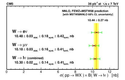
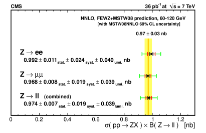
Figure 25: Summary of the $\mathrm{W}$ and $\mathrm{Z}$ production cross section times branching ratio measurements. Measurements in the electron and muon channels, and combined, are compared to the theoretical predictions (yellow band) computed at the NNLO in QCD with recent PDF sets. Statistical uncertainties are represented as a black error bars, while the red error bars also include systematic uncertainties, and the green error bars also include luminosity uncertainties.

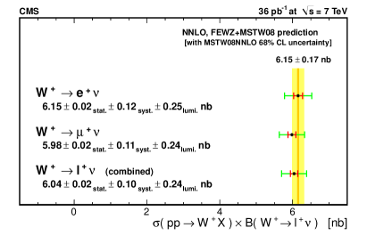
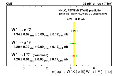
Figure 26: Summary of the $\mathrm{W^{+}}$ and $\mathrm{W^{-}}$ production cross section times branching ratio measurements. Measurements in the electron and muon channels, and combined, are compared to the theoretical predictions computed at the NNLO in QCD with recent PDF sets. Statistical uncertainties are negligible in this plot; the red error bars represent systematic uncertainties, and the green error bars also include luminosity uncertainties.

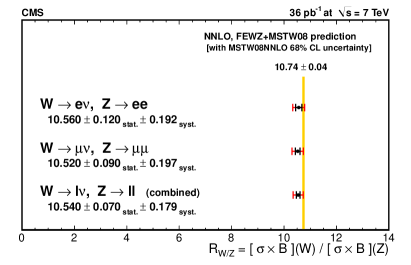
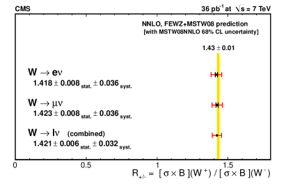
Figure 27: Summary of the measurements of the ratios of W to Z and $\mathrm{W^{+}}$ to $\mathrm{W^{-}}$ production cross sections. Measurements in the electron and muon channels, and combined, are compared to the theoretical predictions computed at the NNLO in QCD with recent PDF sets. Statistical uncertainties are represented as a black error bars, while the red error bars also include systematic uncertainties. Luminosity uncertainties cancel in the ratios.

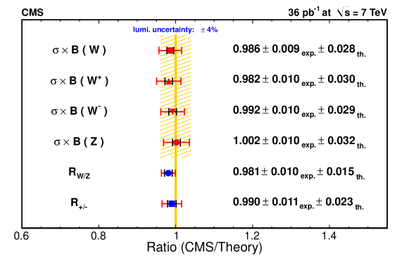
Figure 28: Summary of ratios of the CMS measurements to the theoretical predictions. The experimental uncertainties are represented as black error bars, while the red error bars also include the combining of theoretical uncertainties on the predictions and measured quantities. The yellow band around the vertical yellow line at one represent the luminosity uncertainty (4%) that affects the cross-section measurements.

Table 19: Summary of ratios of CMS measurements to the theoretical predictions.

Quantity	Ratio (CMS/Theory)
$\sigma\times{\cal B}(\Wpm)$	$0.986\pm 0.009\,{\mathrm{(exp)}}\pm 0.028\,{\mathrm{(th)}}\,\,[\pm 0.029\,{\mathrm{(tot)}}]$
$\sigma\times{\cal B}(\mathrm{W^{+}})$	$0.982\pm 0.010\,{\mathrm{(exp)}}\pm 0.030\,{\mathrm{(th)}}\,\,[\pm 0.031\,{\mathrm{(tot)}}]$
$\sigma\times{\cal B}(\mathrm{W^{-}})$	$0.992\pm 0.010\,{\mathrm{(exp)}}\pm 0.029\,{\mathrm{(th)}}\,\,[\pm 0.031\,{\mathrm{(tot)}}]$
$\sigma\times{\cal B}(\mathrm{Z})$	$1.002\pm 0.010\,{\mathrm{(exp)}}\pm 0.032\,{\mathrm{(th)}}\,\,[\pm 0.034\,{\mathrm{(tot)}}]$
$\sigma\times{\cal B}(\mathrm{W})/\sigma\times{\cal B}(\mathrm{Z})$	$0.981\pm 0.010\,{\mathrm{(exp)}}\pm 0.015\,{\mathrm{(th)}}\,\,[\pm 0.018\,{\mathrm{(tot)}}]$
$\sigma\times{\cal B}(\mathrm{W^{+}})/\sigma\times{\cal B}(\mathrm{W^{-}})$	$0.990\pm 0.011\,{\mathrm{(exp)}}\pm 0.023\,{\mathrm{(th)}}\,\,[\pm 0.025\,{\mathrm{(tot)}}]$

Figure 29 shows the CMS W and Z cross section measurements together with measurements at lower center-of-mass energy hadron colliders. The predicted increase of the cross sections with center of mass energy is confirmed by our measurements.

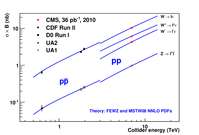
Figure 29: Measurements of inclusive W and Z production cross sections times branching ratios as a function of center-of-mass energy for CMS and experiments at lower-energy colliders. The lines are the NNLO theory predictions.

Table 20 reports the cross sections as measured within the fiducial and kinematic acceptance, thereby eliminating the PDF uncertainties from the results. In effect, these uncertainties are transferred to the theoretical predictions, allowing for a cleaner separation of experimental and theoretical uncertainties. For each channel the fiducial and kinematic acceptance is defined as the fraction of events with lepton $p_{\mathrm{T}}$ greater than $25~{}\GeV$ ($20~{}\GeV$ for $\mathrm{Z}\rightarrow\MM$), including no final-state QED radiation, and with pseudorapidity in the range $|\eta|<2.5$ for electrons and $|\eta|<2.1$ for muons.

Table 20: Summary of production cross section measurements in restricted fiducial and kinematic acceptances. The $p_{\mathrm{T}}$ and $|\eta|$ requirements restricting the acceptance for electrons and muons, and the resulting acceptance values, are also given. The quoted uncertainties on the acceptances (evaluated without FSR effect) are due to the PDF uncertainties.

Channel	$\sigma\times{\cal B}$ in acceptance $A$ (nb)	$A$
$\mathrm{W}\rightarrow\mathrm{e}\nu$	$5.688\pm 0.016\,\mathrm{(stat.)}\pm 0.096\,\mathrm{(syst.)}\pm 0.228\,\mathrm{(lumi.)}$	$0.543\pm 0.003$
$\mathrm{W^{+}}\rightarrow\mathrm{e}^{+}\nu$	$3.404\pm 0.012\,\mathrm{(stat.)}\pm 0.067\,\mathrm{(syst.)}\pm 0.136\,\mathrm{(lumi.)}$	$0.554\pm 0.004$	$p_{\mathrm{T}}>25\GeV$
$\mathrm{W^{-}}\rightarrow\mathrm{e}^{-}\overline{\nu}$	$2.284\pm 0.010\,\mathrm{(stat.)}\pm 0.043\,\mathrm{(syst.)}\pm 0.091\,\mathrm{(lumi.)}$	$0.527\pm 0.006$	$|\eta|<2.5$
$\mathrm{Z}\rightarrow\mathrm{e}^{+}\mathrm{e}^{-}$	$0.452\pm 0.005\,\mathrm{(stat.)}\pm 0.010\,\mathrm{(syst.)}\pm 0.018\,\mathrm{(lumi.)}$	$0.456\pm 0.004$
$\mathrm{W}\rightarrow\mu\nu$	$4.736\pm 0.012\,(\textrm{stat.})\pm 0.067\,(\textrm{syst.})\pm 0.189\,(\textrm{lumi.})$	$0.465\pm 0.004$	$p_{\mathrm{T}}>25\GeV$ $|\eta|<2.1$
$\mathrm{W^{+}}\rightarrow\mu^{+}\nu$	$2.815\pm 0.009\,(\textrm{stat.})\pm 0.042\,(\textrm{syst.})\pm 0.113\,(\textrm{lumi.})$	$0.471\pm 0.004$
$\mathrm{W^{-}}\rightarrow\mu^{-}\overline{\nu}$	$1.921\pm 0.008\,(\textrm{stat.})\pm 0.027\,(\textrm{syst.})\pm 0.077\,(\textrm{lumi.})$	$0.457\pm 0.007$
$\mathrm{Z}\rightarrow\MM$	$0.396\pm 0.003\,\mathrm{(stat.)}\pm 0.007\,\mathrm{(syst.)}\pm 0.016\,\mathrm{(lumi.)}$	$0.409\pm 0.005$	$p_{\mathrm{T}}>20\GeV$
			$|\eta|<2.1$

0.10.1 Extraction of ${\cal B}(\mathrm{W}\rightarrow\ell\nu)$ and $\Gamma(\mathrm{W})$

The precise value of the ratio of the W and Z cross sections obtained from the combination of the measurements in the electron and muon final states can be used to determine the SM parameters ${\cal B}(\mathrm{W}\rightarrow\ell\nu)$ and $\Gamma(\mathrm{W})$.

The ratio of W and Z cross sections can be written as

$$R=\frac{\sigma(\mathrm{pp}\rightarrow\mathrm{W}X)}{\sigma(\mathrm{pp}\rightarrow\mathrm{Z}X)}\,\,\frac{{\cal B}(\mathrm{W}\rightarrow\ell\nu)}{{\cal B}(\mathrm{Z}\rightarrow\ell^{+}\ell^{-})}\,.$$

In order to estimate the value of ${\cal B}(\mathrm{W}\rightarrow\ell\nu)$ the predicted ratio of the W and Z production cross sections and the measured value of the ${\cal B}(\mathrm{Z}\rightarrow\ell^{+}\ell^{-})$ are needed. The NNLO prediction of the ratio, based on the MSTW08 PDFs, is $\sigma_{\mathrm{W}}$/$\sigma_{\mathrm{Z}}$ = 3.34 $\pm$ 0.08. The current measured value for ${\cal B}(\mathrm{Z}\rightarrow\ell^{+}\ell^{-})$ is 0.033658$\pm$0.000023  [63]. Those values lead to an indirect estimation of

$${\cal B}(\mathrm{W}\rightarrow\ell\nu)=0.106\pm 0.003\,,$$

in agreement with the measured value, ${\cal B}(\mathrm{W}\rightarrow\ell\nu)=0.1080\pm 0.0009$ [63].

Using the SM value for the leptonic partial width, $\Gamma(\mathrm{W}\rightarrow\ell\nu)=226.6\pm 0.2$ MeV [64, 65], an indirect measurement of the total $\Gamma(\mathrm{W})$ can be obtained through the formula

$${\cal B}(\mathrm{W}\rightarrow\ell\nu)=\frac{\Gamma(\mathrm{W}\rightarrow\ell\nu)}{\Gamma(\mathrm{W})}\,.$$

Based on the above values we obtain

$$\Gamma(\mathrm{W})=2144\pm 62~{}~{}\mathrm{MeV}\,.$$

The SM prediction is 2093 $\pm$ 2 MeV [65] and the world average of experimental results is 2085 $\pm$ 42 MeV [63]. The indirect measurement of $\Gamma(\mathrm{W})$ is in good agreement with the world average and the theoretical prediction, as well as other published measurements.

0.11 Summary

Measurements of the inclusive $\mathrm{W}$ and $\mathrm{Z}$ production cross sections have been performed using a data sample of pp collision events at $\sqrt{s}=7\TeV$ collected with the CMS detector at the LHC in 2010 and corresponding to an integrated luminosity of 36 pb^-1. The inclusive production cross sections of $\mathrm{W^{+}}$ and $\mathrm{W^{-}}$ have been measured separately as well as the ratios of the $\mathrm{W^{+}}/\mathrm{W^{-}}$ and $\mathrm{W}/\mathrm{Z}$ production cross sections. All measurements are dominated by systematic uncertainties, the main uncertainty originating from the integrated luminosity (4%), which cancels in the ratios. Experimental systematic uncertainties range from 0.7 to 1.8%, and theoretical uncertainties range from 0.9 to 2.1%. The measurement of the $\mathrm{W}/\mathrm{Z}$ cross-section ratio also leads to an indirect determination of $\Gamma(\mathrm{W})$, which is in agreement with the current world average.

The results agree with the ATLAS measurement [20] and with previous CMS results [21]. All measurements are consistent with the SM NNLO predictions.

.12 The CMS Collaboration

Yerevan Physics Institute, Yerevan, Armenia
S. Chatrchyan, V. Khachatryan, A.M. Sirunyan, A. Tumasyan Institut für Hochenergiephysik der OeAW, Wien, Austria
W. Adam, T. Bergauer, M. Dragicevic, J. Erö, C. Fabjan, M. Friedl, R. Frühwirth, V.M. Ghete, J. Hammer1, S. Hänsel, M. Hoch, N. Hörmann, J. Hrubec, M. Jeitler, W. Kiesenhofer, M. Krammer, D. Liko, I. Mikulec, M. Pernicka, B. Rahbaran, H. Rohringer, R. Schöfbeck, J. Strauss, A. Taurok, F. Teischinger, P. Wagner, W. Waltenberger, G. Walzel, E. Widl, C.-E. Wulz National Centre for Particle and High Energy Physics, Minsk, Belarus
V. Mossolov, N. Shumeiko, J. Suarez Gonzalez Universiteit Antwerpen, Antwerpen, Belgium
S. Bansal, L. Benucci, E.A. De Wolf, X. Janssen, T. Maes, L. Mucibello, S. Ochesanu, B. Roland, R. Rougny, M. Selvaggi, H. Van Haevermaet, P. Van Mechelen, N. Van Remortel Vrije Universiteit Brussel, Brussel, Belgium
F. Blekman, S. Blyweert, J. D’Hondt, O. Devroede, R. Gonzalez Suarez, A. Kalogeropoulos, M. Maes, W. Van Doninck, P. Van Mulders, G.P. Van Onsem, I. Villella Université Libre de Bruxelles, Bruxelles, Belgium
O. Charaf, B. Clerbaux, G. De Lentdecker, V. Dero, A.P.R. Gay, G.H. Hammad, T. Hreus, P.E. Marage, A. Raval, L. Thomas, C. Vander Velde, P. Vanlaer Ghent University, Ghent, Belgium
V. Adler, A. Cimmino, S. Costantini, M. Grunewald, B. Klein, J. Lellouch, A. Marinov, J. Mccartin, D. Ryckbosch, F. Thyssen, M. Tytgat, L. Vanelderen, P. Verwilligen, S. Walsh, N. Zaganidis Université Catholique de Louvain, Louvain-la-Neuve, Belgium
S. Basegmez, G. Bruno, J. Caudron, L. Ceard, E. Cortina Gil, J. De Favereau De Jeneret, C. Delaere, D. Favart, A. Giammanco, G. Grégoire, J. Hollar, V. Lemaitre, J. Liao, O. Militaru, C. Nuttens, S. Ovyn, D. Pagano, A. Pin, K. Piotrzkowski, N. Schul Université de Mons, Mons, Belgium
N. Beliy, T. Caebergs, E. Daubie Centro Brasileiro de Pesquisas Fisicas, Rio de Janeiro, Brazil
G.A. Alves, L. Brito, D. De Jesus Damiao, M.E. Pol, M.H.G. Souza Universidade do Estado do Rio de Janeiro, Rio de Janeiro, Brazil
W.L. Aldá Júnior, W. Carvalho, E.M. Da Costa, C. De Oliveira Martins, S. Fonseca De Souza, L. Mundim, H. Nogima, V. Oguri, W.L. Prado Da Silva, A. Santoro, S.M. Silva Do Amaral, A. Sznajder Instituto de Fisica Teorica, Universidade Estadual Paulista, Sao Paulo, Brazil
C.A. Bernardes2, F.A. Dias, T.R. Fernandez Perez Tomei, E. M. Gregores2, C. Lagana, F. Marinho, P.G. Mercadante2, S.F. Novaes, Sandra S. Padula Institute for Nuclear Research and Nuclear Energy, Sofia, Bulgaria
N. Darmenov1, V. Genchev1, P. Iaydjiev1, S. Piperov, M. Rodozov, S. Stoykova, G. Sultanov, V. Tcholakov, R. Trayanov University of Sofia, Sofia, Bulgaria
A. Dimitrov, R. Hadjiiska, A. Karadzhinova, V. Kozhuharov, L. Litov, M. Mateev, B. Pavlov, P. Petkov Institute of High Energy Physics, Beijing, China
J.G. Bian, G.M. Chen, H.S. Chen, C.H. Jiang, D. Liang, S. Liang, X. Meng, J. Tao, J. Wang, J. Wang, X. Wang, Z. Wang, H. Xiao, M. Xu, J. Zang, Z. Zhang State Key Lab. of Nucl. Phys. and Tech.,  Peking University, Beijing, China
Y. Ban, S. Guo, Y. Guo, W. Li, Y. Mao, S.J. Qian, H. Teng, B. Zhu, W. Zou Universidad de Los Andes, Bogota, Colombia
A. Cabrera, B. Gomez Moreno, A.A. Ocampo Rios, A.F. Osorio Oliveros, J.C. Sanabria Technical University of Split, Split, Croatia
N. Godinovic, D. Lelas, K. Lelas, R. Plestina3, D. Polic, I. Puljak University of Split, Split, Croatia
Z. Antunovic, M. Dzelalija Institute Rudjer Boskovic, Zagreb, Croatia
V. Brigljevic, S. Duric, K. Kadija, S. Morovic University of Cyprus, Nicosia, Cyprus
A. Attikis, M. Galanti, J. Mousa, C. Nicolaou, F. Ptochos, P.A. Razis Charles University, Prague, Czech Republic
M. Finger, M. Finger Jr. Academy of Scientific Research and Technology of the Arab Republic of Egypt, Egyptian Network of High Energy Physics, Cairo, Egypt
Y. Assran4, A. Ellithi Kamel, S. Khalil5, M.A. Mahmoud6 National Institute of Chemical Physics and Biophysics, Tallinn, Estonia
A. Hektor, M. Kadastik, M. Müntel, M. Raidal, L. Rebane, A. Tiko Department of Physics, University of Helsinki, Helsinki, Finland
V. Azzolini, P. Eerola, G. Fedi Helsinki Institute of Physics, Helsinki, Finland
S. Czellar, J. Härkönen, A. Heikkinen, V. Karimäki, R. Kinnunen, M.J. Kortelainen, T. Lampén, K. Lassila-Perini, S. Lehti, T. Lindén, P. Luukka, T. Mäenpää, E. Tuominen, J. Tuominiemi, E. Tuovinen, D. Ungaro, L. Wendland Lappeenranta University of Technology, Lappeenranta, Finland
K. Banzuzi, A. Karjalainen, A. Korpela, T. Tuuva Laboratoire d’Annecy-le-Vieux de Physique des Particules, IN2P3-CNRS, Annecy-le-Vieux, France
D. Sillou DSM/IRFU, CEA/Saclay, Gif-sur-Yvette, France
M. Besancon, S. Choudhury, M. Dejardin, D. Denegri, B. Fabbro, J.L. Faure, F. Ferri, S. Ganjour, F.X. Gentit, A. Givernaud, P. Gras, G. Hamel de Monchenault, P. Jarry, E. Locci, J. Malcles, M. Marionneau, L. Millischer, J. Rander, A. Rosowsky, I. Shreyber, M. Titov, P. Verrecchia Laboratoire Leprince-Ringuet, Ecole Polytechnique, IN2P3-CNRS, Palaiseau, France
S. Baffioni, F. Beaudette, L. Benhabib, L. Bianchini, M. Bluj7, C. Broutin, P. Busson, C. Charlot, T. Dahms, L. Dobrzynski, S. Elgammal, R. Granier de Cassagnac, M. Haguenauer, P. Miné, C. Mironov, C. Ochando, P. Paganini, D. Sabes, R. Salerno, Y. Sirois, C. Thiebaux, B. Wyslouch8, A. Zabi Institut Pluridisciplinaire Hubert Curien, Université de Strasbourg, Université de Haute Alsace Mulhouse, CNRS/IN2P3, Strasbourg, France
J.-L. Agram9, J. Andrea, D. Bloch, D. Bodin, J.-M. Brom, M. Cardaci, E.C. Chabert, C. Collard, E. Conte9, F. Drouhin9, C. Ferro, J.-C. Fontaine9, D. Gelé, U. Goerlach, S. Greder, P. Juillot, M. Karim9, A.-C. Le Bihan, Y. Mikami, P. Van Hove Centre de Calcul de l’Institut National de Physique Nucleaire et de Physique des Particules (IN2P3),  Villeurbanne, France
F. Fassi, D. Mercier Université de Lyon, Université Claude Bernard Lyon 1,  CNRS-IN2P3, Institut de Physique Nucléaire de Lyon, Villeurbanne, France
C. Baty, S. Beauceron, N. Beaupere, M. Bedjidian, O. Bondu, G. Boudoul, D. Boumediene, H. Brun, J. Chasserat, R. Chierici, D. Contardo, P. Depasse, H. El Mamouni, J. Fay, S. Gascon, B. Ille, T. Kurca, T. Le Grand, M. Lethuillier, L. Mirabito, S. Perries, V. Sordini, S. Tosi, Y. Tschudi, P. Verdier Institute of High Energy Physics and Informatization, Tbilisi State University, Tbilisi, Georgia
D. Lomidze RWTH Aachen University, I. Physikalisches Institut, Aachen, Germany
G. Anagnostou, S. Beranek, M. Edelhoff, L. Feld, N. Heracleous, O. Hindrichs, R. Jussen, K. Klein, J. Merz, N. Mohr, A. Ostapchuk, A. Perieanu, F. Raupach, J. Sammet, S. Schael, D. Sprenger, H. Weber, M. Weber, B. Wittmer RWTH Aachen University, III. Physikalisches Institut A,  Aachen, Germany
M. Ata, E. Dietz-Laursonn, M. Erdmann, T. Hebbeker, C. Heidemann, A. Hinzmann, K. Hoepfner, T. Klimkovich, D. Klingebiel, P. Kreuzer, D. Lanske${}^{\textrm{\textdagger}}$, J. Lingemann, C. Magass, M. Merschmeyer, A. Meyer, P. Papacz, H. Pieta, H. Reithler, S.A. Schmitz, L. Sonnenschein, J. Steggemann, D. Teyssier RWTH Aachen University, III. Physikalisches Institut B,  Aachen, Germany
M. Bontenackels, M. Davids, M. Duda, G. Flügge, H. Geenen, M. Giffels, W. Haj Ahmad, D. Heydhausen, F. Hoehle, B. Kargoll, T. Kress, Y. Kuessel, A. Linn, A. Nowack, L. Perchalla, O. Pooth, J. Rennefeld, P. Sauerland, A. Stahl, M. Thomas, D. Tornier, M.H. Zoeller Deutsches Elektronen-Synchrotron, Hamburg, Germany
M. Aldaya Martin, W. Behrenhoff, U. Behrens, M. Bergholz10, A. Bethani, K. Borras, A. Cakir, A. Campbell, E. Castro, D. Dammann, G. Eckerlin, D. Eckstein, A. Flossdorf, G. Flucke, A. Geiser, J. Hauk, H. Jung1, M. Kasemann, I. Katkov11, P. Katsas, C. Kleinwort, H. Kluge, A. Knutsson, M. Krämer, D. Krücker, E. Kuznetsova, W. Lange, W. Lohmann10, R. Mankel, M. Marienfeld, I.-A. Melzer-Pellmann, A.B. Meyer, J. Mnich, A. Mussgiller, J. Olzem, A. Petrukhin, D. Pitzl, A. Raspereza, M. Rosin, R. Schmidt10, T. Schoerner-Sadenius, N. Sen, A. Spiridonov, M. Stein, J. Tomaszewska, R. Walsh, C. Wissing University of Hamburg, Hamburg, Germany
C. Autermann, V. Blobel, S. Bobrovskyi, J. Draeger, H. Enderle, U. Gebbert, M. Görner, T. Hermanns, K. Kaschube, G. Kaussen, H. Kirschenmann, R. Klanner, J. Lange, B. Mura, S. Naumann-Emme, F. Nowak, N. Pietsch, C. Sander, H. Schettler, P. Schleper, E. Schlieckau, M. Schröder, T. Schum, H. Stadie, G. Steinbrück, J. Thomsen Institut für Experimentelle Kernphysik, Karlsruhe, Germany
C. Barth, J. Bauer, J. Berger, V. Buege, T. Chwalek, W. De Boer, A. Dierlamm, G. Dirkes, M. Feindt, J. Gruschke, C. Hackstein, F. Hartmann, M. Heinrich, H. Held, K.H. Hoffmann, S. Honc, J.R. Komaragiri, T. Kuhr, D. Martschei, S. Mueller, Th. Müller, M. Niegel, O. Oberst, A. Oehler, J. Ott, T. Peiffer, G. Quast, K. Rabbertz, F. Ratnikov, N. Ratnikova, M. Renz, C. Saout, A. Scheurer, P. Schieferdecker, F.-P. Schilling, G. Schott, H.J. Simonis, F.M. Stober, D. Troendle, J. Wagner-Kuhr, T. Weiler, M. Zeise, V. Zhukov11, E.B. Ziebarth Institute of Nuclear Physics ”Demokritos”,  Aghia Paraskevi, Greece
G. Daskalakis, T. Geralis, S. Kesisoglou, A. Kyriakis, D. Loukas, I. Manolakos, A. Markou, C. Markou, C. Mavrommatis, E. Ntomari, E. Petrakou University of Athens, Athens, Greece
L. Gouskos, T.J. Mertzimekis, A. Panagiotou, N. Saoulidou, E. Stiliaris University of Ioánnina, Ioánnina, Greece
I. Evangelou, C. Foudas, P. Kokkas, N. Manthos, I. Papadopoulos, V. Patras, F.A. Triantis KFKI Research Institute for Particle and Nuclear Physics, Budapest, Hungary
A. Aranyi, G. Bencze, L. Boldizsar, C. Hajdu1, P. Hidas, D. Horvath12, A. Kapusi, K. Krajczar13, F. Sikler1, G.I. Veres13, G. Vesztergombi13 Institute of Nuclear Research ATOMKI, Debrecen, Hungary
N. Beni, J. Molnar, J. Palinkas, Z. Szillasi, V. Veszpremi University of Debrecen, Debrecen, Hungary
P. Raics, Z.L. Trocsanyi, B. Ujvari Panjab University, Chandigarh, India
S.B. Beri, V. Bhatnagar, N. Dhingra, R. Gupta, M. Jindal, M. Kaur, J.M. Kohli, M.Z. Mehta, N. Nishu, L.K. Saini, A. Sharma, A.P. Singh, J. Singh, S.P. Singh University of Delhi, Delhi, India
S. Ahuja, B.C. Choudhary, P. Gupta, S. Jain, A. Kumar, A. Kumar, M. Naimuddin, K. Ranjan, R.K. Shivpuri Saha Institute of Nuclear Physics, Kolkata, India
S. Banerjee, S. Bhattacharya, S. Dutta, B. Gomber, S. Jain, R. Khurana, S. Sarkar Bhabha Atomic Research Centre, Mumbai, India
R.K. Choudhury, D. Dutta, S. Kailas, V. Kumar, P. Mehta, A.K. Mohanty1, L.M. Pant, P. Shukla Tata Institute of Fundamental Research - EHEP, Mumbai, India
T. Aziz, M. Guchait14, A. Gurtu, M. Maity15, D. Majumder, G. Majumder, K. Mazumdar, G.B. Mohanty, A. Saha, K. Sudhakar, N. Wickramage Tata Institute of Fundamental Research - HECR, Mumbai, India
S. Banerjee, S. Dugad, N.K. Mondal Institute for Research and Fundamental Sciences (IPM),  Tehran, Iran
H. Arfaei, H. Bakhshiansohi16, S.M. Etesami, A. Fahim16, M. Hashemi, H. Hesari, A. Jafari16, M. Khakzad, A. Mohammadi17, M. Mohammadi Najafabadi, S. Paktinat Mehdiabadi, B. Safarzadeh, M. Zeinali18 INFN Sezione di Bari ^a, Università di Bari ^b, Politecnico di Bari ^c,  Bari, Italy
M. Abbrescia^a,b, L. Barbone^a,b, C. Calabria^a,b, A. Colaleo^a, D. Creanza^a,c, N. De Filippis^a,c,1, M. De Palma^a,b, L. Fiore^a, G. Iaselli^a,c, L. Lusito^a,b, G. Maggi^a,c, M. Maggi^a, N. Manna^a,b, B. Marangelli^a,b, S. My^a,c, S. Nuzzo^a,b, N. Pacifico^a,b, G.A. Pierro^a, A. Pompili^a,b, G. Pugliese^a,c, F. Romano^a,c, G. Roselli^a,b, G. Selvaggi^a,b, L. Silvestris^a, R. Trentadue^a, S. Tupputi^a,b, G. Zito^a INFN Sezione di Bologna ^a, Università di Bologna ^b,  Bologna, Italy
G. Abbiendi^a, A.C. Benvenuti^a, D. Bonacorsi^a, S. Braibant-Giacomelli^a,b, L. Brigliadori^a, P. Capiluppi^a,b, A. Castro^a,b, F.R. Cavallo^a, M. Cuffiani^a,b, G.M. Dallavalle^a, F. Fabbri^a, A. Fanfani^a,b, D. Fasanella^a, P. Giacomelli^a, M. Giunta^a, C. Grandi^a, S. Marcellini^a, G. Masetti^b, M. Meneghelli^a,b, A. Montanari^a, F.L. Navarria^a,b, F. Odorici^a, A. Perrotta^a, F. Primavera^a, A.M. Rossi^a,b, T. Rovelli^a,b, G. Siroli^a,b, R. Travaglini^a,b INFN Sezione di Catania ^a, Università di Catania ^b,  Catania, Italy
S. Albergo^a,b, G. Cappello^a,b, M. Chiorboli^a,b,1, S. Costa^a,b, R. Potenza^a,b, A. Tricomi^a,b, C. Tuve^a,b INFN Sezione di Firenze ^a, Università di Firenze ^b,  Firenze, Italy
G. Barbagli^a, V. Ciulli^a,b, C. Civinini^a, R. D’Alessandro^a,b, E. Focardi^a,b, S. Frosali^a,b, E. Gallo^a, S. Gonzi^a,b, P. Lenzi^a,b, M. Meschini^a, S. Paoletti^a, G. Sguazzoni^a, A. Tropiano^a,1 INFN Laboratori Nazionali di Frascati, Frascati, Italy
L. Benussi, S. Bianco, S. Colafranceschi19, F. Fabbri, D. Piccolo INFN Sezione di Genova, Genova, Italy
P. Fabbricatore, R. Musenich INFN Sezione di Milano-Bicocca ^a, Università di Milano-Bicocca ^b,  Milano, Italy
A. Benaglia^a,b, F. De Guio^a,b,1, L. Di Matteo^a,b, S. Gennai1, A. Ghezzi^a,b, S. Malvezzi^a, A. Martelli^a,b, A. Massironi^a,b, D. Menasce^a, L. Moroni^a, M. Paganoni^a,b, D. Pedrini^a, S. Ragazzi^a,b, N. Redaelli^a, S. Sala^a, T. Tabarelli de Fatis^a,b INFN Sezione di Napoli ^a, Università di Napoli ”Federico II” ^b,  Napoli, Italy
S. Buontempo^a, C.A. Carrillo Montoya^a,1, N. Cavallo^a,20, A. De Cosa^a,b, F. Fabozzi^a,20, A.O.M. Iorio^a,1, L. Lista^a, M. Merola^a,b, P. Paolucci^a INFN Sezione di Padova ^a, Università di Padova ^b, Università di Trento (Trento) ^c,  Padova, Italy
P. Azzi^a, N. Bacchetta^a, P. Bellan^a,b, D. Bisello^a,b, A. Branca^a, R. Carlin^a,b, P. Checchia^a, T. Dorigo^a, U. Dosselli^a, F. Fanzago^a, F. Gasparini^a,b, U. Gasparini^a,b, A. Gozzelino, S. Lacaprara^a,21, I. Lazzizzera^a,c, M. Margoni^a,b, M. Mazzucato^a, A.T. Meneguzzo^a,b, M. Nespolo^a,1, L. Perrozzi^a,1, N. Pozzobon^a,b, P. Ronchese^a,b, F. Simonetto^a,b, E. Torassa^a, M. Tosi^a,b, S. Vanini^a,b, P. Zotto^a,b, G. Zumerle^a,b INFN Sezione di Pavia ^a, Università di Pavia ^b,  Pavia, Italy
P. Baesso^a,b, U. Berzano^a, S.P. Ratti^a,b, C. Riccardi^a,b, P. Torre^a,b, P. Vitulo^a,b, C. Viviani^a,b INFN Sezione di Perugia ^a, Università di Perugia ^b,  Perugia, Italy
M. Biasini^a,b, G.M. Bilei^a, B. Caponeri^a,b, L. Fanò^a,b, P. Lariccia^a,b, A. Lucaroni^a,b,1, G. Mantovani^a,b, M. Menichelli^a, A. Nappi^a,b, F. Romeo^a,b, A. Santocchia^a,b, S. Taroni^a,b,1, M. Valdata^a,b INFN Sezione di Pisa ^a, Università di Pisa ^b, Scuola Normale Superiore di Pisa ^c,  Pisa, Italy
P. Azzurri^a,c, G. Bagliesi^a, J. Bernardini^a,b, T. Boccali^a,1, G. Broccolo^a,c, R. Castaldi^a, R.T. D’Agnolo^a,c, R. Dell’Orso^a, F. Fiori^a,b, L. Foà^a,c, A. Giassi^a, A. Kraan^a, F. Ligabue^a,c, T. Lomtadze^a, L. Martini^a,22, A. Messineo^a,b, F. Palla^a, F. Palmonari, G. Segneri^a, A.T. Serban^a, P. Spagnolo^a, R. Tenchini^a, G. Tonelli^a,b,1, A. Venturi^a,1, P.G. Verdini^a INFN Sezione di Roma ^a, Università di Roma ”La Sapienza” ^b,  Roma, Italy
L. Barone^a,b, F. Cavallari^a, D. Del Re^a,b, E. Di Marco^a,b, M. Diemoz^a, D. Franci^a,b, M. Grassi^a,1, E. Longo^a,b, P. Meridiani, S. Nourbakhsh^a, G. Organtini^a,b, F. Pandolfi^a,b,1, R. Paramatti^a, S. Rahatlou^a,b, C. Rovelli1 INFN Sezione di Torino ^a, Università di Torino ^b, Università del Piemonte Orientale (Novara) ^c,  Torino, Italy
N. Amapane^a,b, R. Arcidiacono^a,c, S. Argiro^a,b, M. Arneodo^a,c, C. Biino^a, C. Botta^a,b,1, N. Cartiglia^a, R. Castello^a,b, M. Costa^a,b, N. Demaria^a, A. Graziano^a,b,1, C. Mariotti^a, M. Marone^a,b, S. Maselli^a, E. Migliore^a,b, G. Mila^a,b, V. Monaco^a,b, M. Musich^a,b, M.M. Obertino^a,c, N. Pastrone^a, M. Pelliccioni^a,b, A. Potenza^a,b, A. Romero^a,b, M. Ruspa^a,c, R. Sacchi^a,b, V. Sola^a,b, A. Solano^a,b, A. Staiano^a, A. Vilela Pereira^a INFN Sezione di Trieste ^a, Università di Trieste ^b,  Trieste, Italy
S. Belforte^a, F. Cossutti^a, G. Della Ricca^a,b, B. Gobbo^a, D. Montanino^a,b, A. Penzo^a Kangwon National University, Chunchon, Korea
S.G. Heo, S.K. Nam Kyungpook National University, Daegu, Korea
S. Chang, J. Chung, D.H. Kim, G.N. Kim, J.E. Kim, D.J. Kong, H. Park, S.R. Ro, D.C. Son, T. Son Chonnam National University, Institute for Universe and Elementary Particles, Kwangju, Korea
Zero Kim, J.Y. Kim, S. Song Korea University, Seoul, Korea
S. Choi, B. Hong, M. Jo, H. Kim, J.H. Kim, T.J. Kim, K.S. Lee, D.H. Moon, S.K. Park, K.S. Sim University of Seoul, Seoul, Korea
M. Choi, S. Kang, H. Kim, C. Park, I.C. Park, S. Park, G. Ryu Sungkyunkwan University, Suwon, Korea
Y. Choi, Y.K. Choi, J. Goh, M.S. Kim, B. Lee, J. Lee, S. Lee, H. Seo, I. Yu Vilnius University, Vilnius, Lithuania
M.J. Bilinskas, I. Grigelionis, M. Janulis, D. Martisiute, P. Petrov, M. Polujanskas, T. Sabonis Centro de Investigacion y de Estudios Avanzados del IPN, Mexico City, Mexico
H. Castilla-Valdez, E. De La Cruz-Burelo, I. Heredia-de La Cruz, R. Lopez-Fernandez, R. Magaña Villalba, A. Sánchez-Hernández, L.M. Villasenor-Cendejas Universidad Iberoamericana, Mexico City, Mexico
S. Carrillo Moreno, F. Vazquez Valencia Benemerita Universidad Autonoma de Puebla, Puebla, Mexico
H.A. Salazar Ibarguen Universidad Autónoma de San Luis Potosí,  San Luis Potosí,  Mexico
E. Casimiro Linares, A. Morelos Pineda, M.A. Reyes-Santos University of Auckland, Auckland, New Zealand
D. Krofcheck, J. Tam University of Canterbury, Christchurch, New Zealand
P.H. Butler, R. Doesburg, H. Silverwood National Centre for Physics, Quaid-I-Azam University, Islamabad, Pakistan
M. Ahmad, I. Ahmed, M.I. Asghar, H.R. Hoorani, W.A. Khan, T. Khurshid, S. Qazi Institute of Experimental Physics, Faculty of Physics, University of Warsaw, Warsaw, Poland
G. Brona, M. Cwiok, W. Dominik, K. Doroba, A. Kalinowski, M. Konecki, J. Krolikowski Soltan Institute for Nuclear Studies, Warsaw, Poland
T. Frueboes, R. Gokieli, M. Górski, M. Kazana, K. Nawrocki, K. Romanowska-Rybinska, M. Szleper, G. Wrochna, P. Zalewski Laboratório de Instrumentação e Física Experimental de Partículas, Lisboa, Portugal
N. Almeida, P. Bargassa, A. David, P. Faccioli, P.G. Ferreira Parracho, M. Gallinaro1, P. Musella, A. Nayak, J. Pela1, P.Q. Ribeiro, J. Seixas, J. Varela Joint Institute for Nuclear Research, Dubna, Russia
S. Afanasiev, I. Belotelov, I. Golutvin, A. Kamenev, V. Karjavin, G. Kozlov, A. Lanev, P. Moisenz, V. Palichik, V. Perelygin, M. Savina, S. Shmatov, V. Smirnov, A. Volodko, A. Zarubin Petersburg Nuclear Physics Institute, Gatchina (St Petersburg),  Russia
V. Golovtsov, Y. Ivanov, V. Kim, P. Levchenko, V. Murzin, V. Oreshkin, I. Smirnov, V. Sulimov, L. Uvarov, S. Vavilov, A. Vorobyev, An. Vorobyev Institute for Nuclear Research, Moscow, Russia
Yu. Andreev, A. Dermenev, S. Gninenko, N. Golubev, M. Kirsanov, N. Krasnikov, V. Matveev, A. Pashenkov, A. Toropin, S. Troitsky Institute for Theoretical and Experimental Physics, Moscow, Russia
V. Epshteyn, V. Gavrilov, V. Kaftanov${}^{\textrm{\textdagger}}$, M. Kossov1, A. Krokhotin, N. Lychkovskaya, V. Popov, G. Safronov, S. Semenov, V. Stolin, E. Vlasov, A. Zhokin Moscow State University, Moscow, Russia
A. Belyaev, E. Boos, M. Dubinin23, L. Dudko, A. Ershov, A. Gribushin, O. Kodolova, I. Lokhtin, A. Markina, S. Obraztsov, M. Perfilov, S. Petrushanko, L. Sarycheva, V. Savrin, A. Snigirev P.N. Lebedev Physical Institute, Moscow, Russia
V. Andreev, M. Azarkin, I. Dremin, M. Kirakosyan, A. Leonidov, S.V. Rusakov, A. Vinogradov State Research Center of Russian Federation, Institute for High Energy Physics, Protvino, Russia
I. Azhgirey, I. Bayshev, S. Bitioukov, V. Grishin1, V. Kachanov, D. Konstantinov, A. Korablev, V. Krychkine, V. Petrov, R. Ryutin, A. Sobol, L. Tourtchanovitch, S. Troshin, N. Tyurin, A. Uzunian, A. Volkov University of Belgrade, Faculty of Physics and Vinca Institute of Nuclear Sciences, Belgrade, Serbia
P. Adzic24, M. Djordjevic, D. Krpic24, J. Milosevic Centro de Investigaciones Energéticas Medioambientales y Tecnológicas (CIEMAT),  Madrid, Spain
M. Aguilar-Benitez, J. Alcaraz Maestre, P. Arce, C. Battilana, E. Calvo, M. Cepeda, M. Cerrada, M. Chamizo Llatas, N. Colino, B. De La Cruz, A. Delgado Peris, C. Diez Pardos, D. Domínguez Vázquez, C. Fernandez Bedoya, J.P. Fernández Ramos, A. Ferrando, J. Flix, M.C. Fouz, P. Garcia-Abia, O. Gonzalez Lopez, S. Goy Lopez, J.M. Hernandez, M.I. Josa, G. Merino, J. Puerta Pelayo, I. Redondo, L. Romero, J. Santaolalla, M.S. Soares, C. Willmott Universidad Autónoma de Madrid, Madrid, Spain
C. Albajar, G. Codispoti, J.F. de Trocóniz Universidad de Oviedo, Oviedo, Spain
J. Cuevas, J. Fernandez Menendez, S. Folgueras, I. Gonzalez Caballero, L. Lloret Iglesias, J.M. Vizan Garcia Instituto de Física de Cantabria (IFCA),  CSIC-Universidad de Cantabria, Santander, Spain
J.A. Brochero Cifuentes, I.J. Cabrillo, A. Calderon, S.H. Chuang, J. Duarte Campderros, M. Felcini25, M. Fernandez, G. Gomez, J. Gonzalez Sanchez, C. Jorda, P. Lobelle Pardo, A. Lopez Virto, J. Marco, R. Marco, C. Martinez Rivero, F. Matorras, F.J. Munoz Sanchez, J. Piedra Gomez26, T. Rodrigo, A.Y. Rodríguez-Marrero, A. Ruiz-Jimeno, L. Scodellaro, M. Sobron Sanudo, I. Vila, R. Vilar Cortabitarte CERN, European Organization for Nuclear Research, Geneva, Switzerland
D. Abbaneo, E. Auffray, G. Auzinger, P. Baillon, A.H. Ball, D. Barney, A.J. Bell27, D. Benedetti, C. Bernet3, W. Bialas, P. Bloch, A. Bocci, S. Bolognesi, M. Bona, H. Breuker, K. Bunkowski, T. Camporesi, G. Cerminara, T. Christiansen, J.A. Coarasa Perez, B. Curé, D. D’Enterria, A. De Roeck, S. Di Guida, N. Dupont-Sagorin, A. Elliott-Peisert, B. Frisch, W. Funk, A. Gaddi, G. Georgiou, H. Gerwig, D. Gigi, K. Gill, D. Giordano, F. Glege, R. Gomez-Reino Garrido, M. Gouzevitch, P. Govoni, S. Gowdy, L. Guiducci, M. Hansen, C. Hartl, J. Harvey, J. Hegeman, B. Hegner, H.F. Hoffmann, A. Honma, V. Innocente, P. Janot, K. Kaadze, E. Karavakis, P. Lecoq, C. Lourenço, T. Mäki, M. Malberti, L. Malgeri, M. Mannelli, L. Masetti, A. Maurisset, F. Meijers, S. Mersi, E. Meschi, R. Moser, M.U. Mozer, M. Mulders, E. Nesvold1, M. Nguyen, T. Orimoto, L. Orsini, E. Palencia Cortezon, E. Perez, A. Petrilli, A. Pfeiffer, M. Pierini, M. Pimiä, D. Piparo, G. Polese, A. Racz, W. Reece, J. Rodrigues Antunes, G. Rolandi28, T. Rommerskirchen, M. Rovere, H. Sakulin, C. Schäfer, C. Schwick, I. Segoni, A. Sharma, P. Siegrist, P. Silva, M. Simon, P. Sphicas29, M. Spiropulu23, M. Stoye, P. Tropea, A. Tsirou, P. Vichoudis, M. Voutilainen, W.D. Zeuner Paul Scherrer Institut, Villigen, Switzerland
W. Bertl, K. Deiters, W. Erdmann, K. Gabathuler, R. Horisberger, Q. Ingram, H.C. Kaestli, S. König, D. Kotlinski, U. Langenegger, F. Meier, D. Renker, T. Rohe, J. Sibille30, A. Starodumov31 Institute for Particle Physics, ETH Zurich, Zurich, Switzerland
L. Bäni, P. Bortignon, L. Caminada32, B. Casal, N. Chanon, Z. Chen, S. Cittolin, G. Dissertori, M. Dittmar, J. Eugster, K. Freudenreich, C. Grab, W. Hintz, P. Lecomte, W. Lustermann, C. Marchica32, P. Martinez Ruiz del Arbol, P. Milenovic33, F. Moortgat, C. Nägeli32, P. Nef, F. Nessi-Tedaldi, L. Pape, F. Pauss, T. Punz, A. Rizzi, F.J. Ronga, M. Rossini, L. Sala, A.K. Sanchez, M.-C. Sawley, B. Stieger, L. Tauscher${}^{\textrm{\textdagger}}$, A. Thea, K. Theofilatos, D. Treille, C. Urscheler, R. Wallny, M. Weber, L. Wehrli, J. Weng Universität Zürich, Zurich, Switzerland
E. Aguilo, C. Amsler, V. Chiochia, S. De Visscher, C. Favaro, M. Ivova Rikova, B. Millan Mejias, P. Otiougova, P. Robmann, A. Schmidt, H. Snoek National Central University, Chung-Li, Taiwan
Y.H. Chang, K.H. Chen, C.M. Kuo, S.W. Li, W. Lin, Z.K. Liu, Y.J. Lu, D. Mekterovic, R. Volpe, J.H. Wu, S.S. Yu National Taiwan University (NTU),  Taipei, Taiwan
P. Bartalini, P. Chang, Y.H. Chang, Y.W. Chang, Y. Chao, K.F. Chen, W.-S. Hou, Y. Hsiung, K.Y. Kao, Y.J. Lei, R.-S. Lu, J.G. Shiu, Y.M. Tzeng, M. Wang Cukurova University, Adana, Turkey
A. Adiguzel, M.N. Bakirci34, S. Cerci35, C. Dozen, I. Dumanoglu, E. Eskut, S. Girgis, G. Gokbulut, I. Hos, E.E. Kangal, A. Kayis Topaksu, G. Onengut, K. Ozdemir, S. Ozturk36, A. Polatoz, K. Sogut37, D. Sunar Cerci35, B. Tali35, H. Topakli34, D. Uzun, L.N. Vergili, M. Vergili Middle East Technical University, Physics Department, Ankara, Turkey
I.V. Akin, T. Aliev, B. Bilin, S. Bilmis, M. Deniz, H. Gamsizkan, A.M. Guler, K. Ocalan, A. Ozpineci, M. Serin, R. Sever, U.E. Surat, E. Yildirim, M. Zeyrek Bogazici University, Istanbul, Turkey
M. Deliomeroglu, D. Demir38, E. Gülmez, B. Isildak, M. Kaya39, O. Kaya39, M. Özbek, S. Ozkorucuklu40, N. Sonmez41 National Scientific Center, Kharkov Institute of Physics and Technology, Kharkov, Ukraine
L. Levchuk University of Bristol, Bristol, United Kingdom
F. Bostock, J.J. Brooke, T.L. Cheng, E. Clement, D. Cussans, R. Frazier, J. Goldstein, M. Grimes, D. Hartley, G.P. Heath, H.F. Heath, L. Kreczko, S. Metson, D.M. Newbold42, K. Nirunpong, A. Poll, S. Senkin, V.J. Smith Rutherford Appleton Laboratory, Didcot, United Kingdom
L. Basso43, K.W. Bell, A. Belyaev43, C. Brew, R.M. Brown, B. Camanzi, D.J.A. Cockerill, J.A. Coughlan, K. Harder, S. Harper, J. Jackson, B.W. Kennedy, E. Olaiya, D. Petyt, B.C. Radburn-Smith, C.H. Shepherd-Themistocleous, I.R. Tomalin, W.J. Womersley, S.D. Worm Imperial College, London, United Kingdom
R. Bainbridge, G. Ball, J. Ballin, R. Beuselinck, O. Buchmuller, D. Colling, N. Cripps, M. Cutajar, G. Davies, M. Della Negra, W. Ferguson, J. Fulcher, D. Futyan, A. Gilbert, A. Guneratne Bryer, G. Hall, Z. Hatherell, J. Hays, G. Iles, M. Jarvis, G. Karapostoli, L. Lyons, B.C. MacEvoy, A.-M. Magnan, J. Marrouche, B. Mathias, R. Nandi, J. Nash, A. Nikitenko31, A. Papageorgiou, M. Pesaresi, K. Petridis, M. Pioppi44, D.M. Raymond, S. Rogerson, N. Rompotis, A. Rose, M.J. Ryan, C. Seez, P. Sharp, A. Sparrow, A. Tapper, S. Tourneur, M. Vazquez Acosta, T. Virdee, S. Wakefield, N. Wardle, D. Wardrope, T. Whyntie Brunel University, Uxbridge, United Kingdom
M. Barrett, M. Chadwick, J.E. Cole, P.R. Hobson, A. Khan, P. Kyberd, D. Leslie, W. Martin, I.D. Reid, L. Teodorescu Baylor University, Waco, USA
K. Hatakeyama, H. Liu The University of Alabama, Tuscaloosa, USA
C. Henderson Boston University, Boston, USA
T. Bose, E. Carrera Jarrin, C. Fantasia, A. Heister, J. St. John, P. Lawson, D. Lazic, J. Rohlf, D. Sperka, L. Sulak Brown University, Providence, USA
A. Avetisyan, S. Bhattacharya, J.P. Chou, D. Cutts, A. Ferapontov, U. Heintz, S. Jabeen, G. Kukartsev, G. Landsberg, M. Luk, M. Narain, D. Nguyen, M. Segala, T. Sinthuprasith, T. Speer, K.V. Tsang University of California, Davis, Davis, USA
R. Breedon, G. Breto, M. Calderon De La Barca Sanchez, S. Chauhan, M. Chertok, J. Conway, P.T. Cox, J. Dolen, R. Erbacher, E. Friis, W. Ko, A. Kopecky, R. Lander, H. Liu, S. Maruyama, T. Miceli, M. Nikolic, D. Pellett, J. Robles, S. Salur, T. Schwarz, M. Searle, J. Smith, M. Squires, M. Tripathi, R. Vasquez Sierra, C. Veelken University of California, Los Angeles, Los Angeles, USA
V. Andreev, K. Arisaka, D. Cline, R. Cousins, A. Deisher, J. Duris, S. Erhan, C. Farrell, J. Hauser, M. Ignatenko, C. Jarvis, C. Plager, G. Rakness, P. Schlein${}^{\textrm{\textdagger}}$, J. Tucker, V. Valuev University of California, Riverside, Riverside, USA
J. Babb, A. Chandra, R. Clare, J. Ellison, J.W. Gary, F. Giordano, G. Hanson, G.Y. Jeng, S.C. Kao, F. Liu, H. Liu, O.R. Long, A. Luthra, H. Nguyen, S. Paramesvaran, B.C. Shen${}^{\textrm{\textdagger}}$, R. Stringer, J. Sturdy, S. Sumowidagdo, R. Wilken, S. Wimpenny University of California, San Diego, La Jolla, USA
W. Andrews, J.G. Branson, G.B. Cerati, D. Evans, F. Golf, A. Holzner, R. Kelley, M. Lebourgeois, J. Letts, B. Mangano, S. Padhi, C. Palmer, G. Petrucciani, H. Pi, M. Pieri, R. Ranieri, M. Sani, V. Sharma, S. Simon, E. Sudano, M. Tadel, Y. Tu, A. Vartak, S. Wasserbaech45, F. Würthwein, A. Yagil, J. Yoo University of California, Santa Barbara, Santa Barbara, USA
D. Barge, R. Bellan, C. Campagnari, M. D’Alfonso, T. Danielson, K. Flowers, P. Geffert, J. Incandela, C. Justus, P. Kalavase, S.A. Koay, D. Kovalskyi, V. Krutelyov, S. Lowette, N. Mccoll, V. Pavlunin, F. Rebassoo, J. Ribnik, J. Richman, R. Rossin, D. Stuart, W. To, J.R. Vlimant California Institute of Technology, Pasadena, USA
A. Apresyan, A. Bornheim, J. Bunn, Y. Chen, M. Gataullin, Y. Ma, A. Mott, H.B. Newman, C. Rogan, K. Shin, V. Timciuc, P. Traczyk, J. Veverka, R. Wilkinson, Y. Yang, R.Y. Zhu Carnegie Mellon University, Pittsburgh, USA
B. Akgun, R. Carroll, T. Ferguson, Y. Iiyama, D.W. Jang, S.Y. Jun, Y.F. Liu, M. Paulini, J. Russ, H. Vogel, I. Vorobiev University of Colorado at Boulder, Boulder, USA
J.P. Cumalat, M.E. Dinardo, B.R. Drell, C.J. Edelmaier, W.T. Ford, A. Gaz, B. Heyburn, E. Luiggi Lopez, U. Nauenberg, J.G. Smith, K. Stenson, K.A. Ulmer, S.R. Wagner, S.L. Zang Cornell University, Ithaca, USA
L. Agostino, J. Alexander, A. Chatterjee, N. Eggert, L.K. Gibbons, B. Heltsley, K. Henriksson, W. Hopkins, A. Khukhunaishvili, B. Kreis, G. Nicolas Kaufman, J.R. Patterson, D. Puigh, A. Ryd, M. Saelim, E. Salvati, X. Shi, W. Sun, W.D. Teo, J. Thom, J. Thompson, J. Vaughan, Y. Weng, L. Winstrom, P. Wittich Fairfield University, Fairfield, USA
A. Biselli, G. Cirino, D. Winn Fermi National Accelerator Laboratory, Batavia, USA
S. Abdullin, M. Albrow, J. Anderson, G. Apollinari, M. Atac, J.A. Bakken, L.A.T. Bauerdick, A. Beretvas, J. Berryhill, P.C. Bhat, I. Bloch, F. Borcherding, K. Burkett, J.N. Butler, V. Chetluru, H.W.K. Cheung, F. Chlebana, S. Cihangir, W. Cooper, D.P. Eartly, V.D. Elvira, S. Esen, I. Fisk, J. Freeman, Y. Gao, E. Gottschalk, D. Green, K. Gunthoti, O. Gutsche, J. Hanlon, R.M. Harris, J. Hirschauer, B. Hooberman, H. Jensen, M. Johnson, U. Joshi, R. Khatiwada, B. Klima, K. Kousouris, S. Kunori, S. Kwan, C. Leonidopoulos, P. Limon, D. Lincoln, R. Lipton, J. Lykken, K. Maeshima, J.M. Marraffino, D. Mason, P. McBride, T. Miao, K. Mishra, S. Mrenna, Y. Musienko46, C. Newman-Holmes, V. O’Dell, J. Pivarski, R. Pordes, O. Prokofyev, E. Sexton-Kennedy, S. Sharma, W.J. Spalding, L. Spiegel, P. Tan, L. Taylor, S. Tkaczyk, L. Uplegger, E.W. Vaandering, R. Vidal, J. Whitmore, W. Wu, F. Yang, F. Yumiceva, J.C. Yun University of Florida, Gainesville, USA
D. Acosta, P. Avery, D. Bourilkov, M. Chen, S. Das, M. De Gruttola, G.P. Di Giovanni, D. Dobur, A. Drozdetskiy, R.D. Field, M. Fisher, Y. Fu, I.K. Furic, J. Gartner, J. Hugon, B. Kim, J. Konigsberg, A. Korytov, A. Kropivnitskaya, T. Kypreos, J.F. Low, K. Matchev, G. Mitselmakher, L. Muniz, C. Prescott, R. Remington, A. Rinkevicius, M. Schmitt, B. Scurlock, P. Sellers, N. Skhirtladze, M. Snowball, D. Wang, J. Yelton, M. Zakaria Florida International University, Miami, USA
V. Gaultney, L.M. Lebolo, S. Linn, P. Markowitz, G. Martinez, J.L. Rodriguez Florida State University, Tallahassee, USA
T. Adams, A. Askew, J. Bochenek, J. Chen, B. Diamond, S.V. Gleyzer, J. Haas, S. Hagopian, V. Hagopian, M. Jenkins, K.F. Johnson, H. Prosper, L. Quertenmont, S. Sekmen, V. Veeraraghavan Florida Institute of Technology, Melbourne, USA
M.M. Baarmand, B. Dorney, S. Guragain, M. Hohlmann, H. Kalakhety, I. Vodopiyanov University of Illinois at Chicago (UIC),  Chicago, USA
M.R. Adams, I.M. Anghel, L. Apanasevich, Y. Bai, V.E. Bazterra, R.R. Betts, J. Callner, R. Cavanaugh, C. Dragoiu, L. Gauthier, C.E. Gerber, D.J. Hofman, S. Khalatyan, G.J. Kunde47, F. Lacroix, M. Malek, C. O’Brien, C. Silkworth, C. Silvestre, A. Smoron, D. Strom, N. Varelas The University of Iowa, Iowa City, USA
U. Akgun, E.A. Albayrak, B. Bilki, W. Clarida, F. Duru, C.K. Lae, E. McCliment, J.-P. Merlo, H. Mermerkaya48, A. Mestvirishvili, A. Moeller, J. Nachtman, C.R. Newsom, E. Norbeck, J. Olson, Y. Onel, F. Ozok, S. Sen, J. Wetzel, T. Yetkin, K. Yi Johns Hopkins University, Baltimore, USA
B.A. Barnett, B. Blumenfeld, A. Bonato, C. Eskew, D. Fehling, G. Giurgiu, A.V. Gritsan, Z.J. Guo, G. Hu, P. Maksimovic, S. Rappoccio, M. Swartz, N.V. Tran, A. Whitbeck The University of Kansas, Lawrence, USA
P. Baringer, A. Bean, G. Benelli, O. Grachov, R.P. Kenny Iii, M. Murray, D. Noonan, S. Sanders, J.S. Wood, V. Zhukova Kansas State University, Manhattan, USA
A.f. Barfuss, T. Bolton, I. Chakaberia, A. Ivanov, S. Khalil, M. Makouski, Y. Maravin, S. Shrestha, I. Svintradze, Z. Wan Lawrence Livermore National Laboratory, Livermore, USA
J. Gronberg, D. Lange, D. Wright University of Maryland, College Park, USA
A. Baden, M. Boutemeur, S.C. Eno, D. Ferencek, J.A. Gomez, N.J. Hadley, R.G. Kellogg, M. Kirn, Y. Lu, A.C. Mignerey, K. Rossato, P. Rumerio, F. Santanastasio, A. Skuja, J. Temple, M.B. Tonjes, S.C. Tonwar, E. Twedt Massachusetts Institute of Technology, Cambridge, USA
B. Alver, G. Bauer, J. Bendavid, W. Busza, E. Butz, I.A. Cali, M. Chan, V. Dutta, P. Everaerts, G. Gomez Ceballos, M. Goncharov, K.A. Hahn, P. Harris, Y. Kim, M. Klute, Y.-J. Lee, W. Li, C. Loizides, P.D. Luckey, T. Ma, S. Nahn, C. Paus, D. Ralph, C. Roland, G. Roland, M. Rudolph, G.S.F. Stephans, F. Stöckli, K. Sumorok, K. Sung, D. Velicanu, E.A. Wenger, R. Wolf, S. Xie, M. Yang, Y. Yilmaz, A.S. Yoon, M. Zanetti University of Minnesota, Minneapolis, USA
S.I. Cooper, P. Cushman, B. Dahmes, A. De Benedetti, P.R. Dudero, G. Franzoni, A. Gude, J. Haupt, K. Klapoetke, Y. Kubota, J. Mans, N. Pastika, V. Rekovic, R. Rusack, M. Sasseville, A. Singovsky, N. Tambe University of Mississippi, University, USA
L.M. Cremaldi, R. Godang, R. Kroeger, L. Perera, R. Rahmat, D.A. Sanders, D. Summers University of Nebraska-Lincoln, Lincoln, USA
K. Bloom, S. Bose, J. Butt, D.R. Claes, A. Dominguez, M. Eads, P. Jindal, J. Keller, T. Kelly, I. Kravchenko, J. Lazo-Flores, H. Malbouisson, S. Malik, G.R. Snow State University of New York at Buffalo, Buffalo, USA
U. Baur, A. Godshalk, I. Iashvili, S. Jain, A. Kharchilava, A. Kumar, S.P. Shipkowski, K. Smith Northeastern University, Boston, USA
G. Alverson, E. Barberis, D. Baumgartel, O. Boeriu, M. Chasco, S. Reucroft, J. Swain, D. Trocino, D. Wood, J. Zhang Northwestern University, Evanston, USA
A. Anastassov, A. Kubik, N. Odell, R.A. Ofierzynski, B. Pollack, A. Pozdnyakov, M. Schmitt, S. Stoynev, M. Velasco, S. Won University of Notre Dame, Notre Dame, USA
L. Antonelli, D. Berry, A. Brinkerhoff, M. Hildreth, C. Jessop, D.J. Karmgard, J. Kolb, T. Kolberg, K. Lannon, W. Luo, S. Lynch, N. Marinelli, D.M. Morse, T. Pearson, R. Ruchti, J. Slaunwhite, N. Valls, M. Wayne, J. Ziegler The Ohio State University, Columbus, USA
B. Bylsma, L.S. Durkin, J. Gu, C. Hill, P. Killewald, K. Kotov, T.Y. Ling, M. Rodenburg, C. Vuosalo, G. Williams Princeton University, Princeton, USA
N. Adam, E. Berry, P. Elmer, D. Gerbaudo, V. Halyo, P. Hebda, A. Hunt, E. Laird, D. Lopes Pegna, D. Marlow, T. Medvedeva, M. Mooney, J. Olsen, P. Piroué, X. Quan, B. Safdi, H. Saka, D. Stickland, C. Tully, J.S. Werner, A. Zuranski University of Puerto Rico, Mayaguez, USA
J.G. Acosta, X.T. Huang, A. Lopez, H. Mendez, S. Oliveros, J.E. Ramirez Vargas, A. Zatserklyaniy Purdue University, West Lafayette, USA
E. Alagoz, V.E. Barnes, G. Bolla, L. Borrello, D. Bortoletto, M. De Mattia, A. Everett, A.F. Garfinkel, L. Gutay, Z. Hu, M. Jones, O. Koybasi, M. Kress, A.T. Laasanen, N. Leonardo, C. Liu, V. Maroussov, P. Merkel, D.H. Miller, N. Neumeister, I. Shipsey, D. Silvers, A. Svyatkovskiy, H.D. Yoo, J. Zablocki, Y. Zheng Purdue University Calumet, Hammond, USA
N. Parashar Rice University, Houston, USA
A. Adair, C. Boulahouache, K.M. Ecklund, F.J.M. Geurts, B.P. Padley, R. Redjimi, J. Roberts, J. Zabel University of Rochester, Rochester, USA
B. Betchart, A. Bodek, Y.S. Chung, R. Covarelli, P. de Barbaro, R. Demina, Y. Eshaq, H. Flacher, A. Garcia-Bellido, P. Goldenzweig, Y. Gotra, J. Han, A. Harel, D.C. Miner, D. Orbaker, G. Petrillo, W. Sakumoto, D. Vishnevskiy, M. Zielinski The Rockefeller University, New York, USA
A. Bhatti, R. Ciesielski, L. Demortier, K. Goulianos, G. Lungu, S. Malik, C. Mesropian Rutgers, the State University of New Jersey, Piscataway, USA
O. Atramentov, A. Barker, D. Duggan, Y. Gershtein, R. Gray, E. Halkiadakis, D. Hidas, D. Hits, A. Lath, S. Panwalkar, R. Patel, K. Rose, S. Schnetzer, S. Somalwar, R. Stone, S. Thomas University of Tennessee, Knoxville, USA
G. Cerizza, M. Hollingsworth, S. Spanier, Z.C. Yang, A. York Texas A&M University, College Station, USA
R. Eusebi, W. Flanagan, J. Gilmore, A. Gurrola, T. Kamon, V. Khotilovich, R. Montalvo, I. Osipenkov, Y. Pakhotin, A. Safonov, S. Sengupta, A. Tatarinov, D. Toback, M. Weinberger Texas Tech University, Lubbock, USA
N. Akchurin, C. Bardak, J. Damgov, C. Jeong, K. Kovitanggoon, S.W. Lee, T. Libeiro, P. Mane, Y. Roh, A. Sill, I. Volobouev, R. Wigmans, E. Yazgan Vanderbilt University, Nashville, USA
E. Appelt, E. Brownson, D. Engh, C. Florez, W. Gabella, M. Issah, W. Johns, P. Kurt, C. Maguire, A. Melo, P. Sheldon, B. Snook, S. Tuo, J. Velkovska University of Virginia, Charlottesville, USA
M.W. Arenton, M. Balazs, S. Boutle, B. Cox, B. Francis, J. Goodell, R. Hirosky, A. Ledovskoy, C. Lin, C. Neu, R. Yohay Wayne State University, Detroit, USA
S. Gollapinni, R. Harr, P.E. Karchin, P. Lamichhane, M. Mattson, C. Milstène, A. Sakharov University of Wisconsin, Madison, USA
M. Anderson, M. Bachtis, J.N. Bellinger, D. Carlsmith, S. Dasu, J. Efron, L. Gray, K.S. Grogg, M. Grothe, R. Hall-Wilton, M. Herndon, A. Hervé, P. Klabbers, J. Klukas, A. Lanaro, C. Lazaridis, J. Leonard, R. Loveless, A. Mohapatra, I. Ojalvo, D. Reeder, I. Ross, A. Savin, W.H. Smith, J. Swanson, M. Weinberg †: Deceased
1:  Also at CERN, European Organization for Nuclear Research, Geneva, Switzerland
2:  Also at Universidade Federal do ABC, Santo Andre, Brazil
3:  Also at Laboratoire Leprince-Ringuet, Ecole Polytechnique, IN2P3-CNRS, Palaiseau, France
4:  Also at Suez Canal University, Suez, Egypt
5:  Also at British University, Cairo, Egypt
6:  Also at Fayoum University, El-Fayoum, Egypt
7:  Also at Soltan Institute for Nuclear Studies, Warsaw, Poland
8:  Also at Massachusetts Institute of Technology, Cambridge, USA
9:  Also at Université de Haute-Alsace, Mulhouse, France
10: Also at Brandenburg University of Technology, Cottbus, Germany
11: Also at Moscow State University, Moscow, Russia
12: Also at Institute of Nuclear Research ATOMKI, Debrecen, Hungary
13: Also at Eötvös Loránd University, Budapest, Hungary
14: Also at Tata Institute of Fundamental Research - HECR, Mumbai, India
15: Also at University of Visva-Bharati, Santiniketan, India
16: Also at Sharif University of Technology, Tehran, Iran
17: Also at Shiraz University, Shiraz, Iran
18: Also at Isfahan University of Technology, Isfahan, Iran
19: Also at Facoltà Ingegneria Università di Roma, Roma, Italy
20: Also at Università della Basilicata, Potenza, Italy
21: Also at Laboratori Nazionali di Legnaro dell’ INFN, Legnaro, Italy
22: Also at Università degli studi di Siena, Siena, Italy
23: Also at California Institute of Technology, Pasadena, USA
24: Also at Faculty of Physics of University of Belgrade, Belgrade, Serbia
25: Also at University of California, Los Angeles, Los Angeles, USA
26: Also at University of Florida, Gainesville, USA
27: Also at Université de Genève, Geneva, Switzerland
28: Also at Scuola Normale e Sezione dell’ INFN, Pisa, Italy
29: Also at University of Athens, Athens, Greece
30: Also at The University of Kansas, Lawrence, USA
31: Also at Institute for Theoretical and Experimental Physics, Moscow, Russia
32: Also at Paul Scherrer Institut, Villigen, Switzerland
33: Also at University of Belgrade, Faculty of Physics and Vinca Institute of Nuclear Sciences, Belgrade, Serbia
34: Also at Gaziosmanpasa University, Tokat, Turkey
35: Also at Adiyaman University, Adiyaman, Turkey
36: Also at The University of Iowa, Iowa City, USA
37: Also at Mersin University, Mersin, Turkey
38: Also at Izmir Institute of Technology, Izmir, Turkey
39: Also at Kafkas University, Kars, Turkey
40: Also at Suleyman Demirel University, Isparta, Turkey
41: Also at Ege University, Izmir, Turkey
42: Also at Rutherford Appleton Laboratory, Didcot, United Kingdom
43: Also at School of Physics and Astronomy, University of Southampton, Southampton, United Kingdom
44: Also at INFN Sezione di Perugia; Università di Perugia, Perugia, Italy
45: Also at Utah Valley University, Orem, USA
46: Also at Institute for Nuclear Research, Moscow, Russia
47: Also at Los Alamos National Laboratory, Los Alamos, USA
48: Also at Erzincan University, Erzincan, Turkey

References

- [1] S.D. Drell and T.M. Yan, “Massive Lepton-Pair Production in Hadron-Hadron Collisions at High Energies”, Phys. Rev. Lett. 25 (1970) 316. doi:10.1103/PhysRevLett.25.316.
- [2] J. Kubar-Andre and F. E. Paige, “Gluon corrections to the Drell–Yan model”, Phys. Rev. D 19 (1979) 221. doi:10.1103/PhysRevD.19.221.
- [3] G. Altarelli, R. Ellis, and G. Martinelli, “Large Perturbative Corrections to the Drell–Yan Process in QCD”, Nucl. Phys. B 157 (1979) 461. doi:10.1016/0550-3213(79)90116-0.
- [4] J. Kubar, M. Le Bellac, J. Meunier et al., “QCD corrections to the Drell–Yan mechanism and the pion structure function”, Nucl. Phys. B 175 (1980) 251. doi:10.1016/0550-3213(80)90053-X.
- [5] P. Rijken and W. van Neerven, “Order contributions to the Drell–Yan cross-section at fixed target energies”, Phys. Rev. D 51 (1995) 44. doi:10.1103/PhysRevD.51.44.
- [6] R. Hamberg, W. van Neerven, and T. Matsuura, “A complete calculation of the order correction to the Drell–Yan -factor”, Nucl. Phys. B 359 (1991) 343. Erratum-ibid. B 644 (2002) 403. doi:10.1016/0550-3213(91)90064-5.
- [7] W. van Neervenand and E. Zijlstra, “The corrected Drell–Yan -factor in the DIS and scheme”, Nucl. Phys. B 382 (1992) 11. Erratum-ibid. B 680 (2004) 513. doi:10.1016/0550-3213(92)90078-P.
- [8] R. Harlander and W. Kilgore, “Next-to-next-to-leading order Higgs production at hadron colliders”, Phys. Rev. Lett. 88 (2002) 201801. doi:10.1103/PhysRevLett.88.201801.
- [9] C. Anastasiou, L. Dixon, K. Melnikov et al., “High precision QCD at hadron colliders: Electroweak gauge boson rapidity distributions at next-to-ntext-to leading order”, Phys. Rev. D 69 (2004) 094008. doi:10.1103/PhysRevD.69.094008.
- [10] H1, ZEUS Collaboration, “Combined measurement and QCD analysis of the inclusive scattering cross sections at HERA”, JHEP 01 (2010) 109. doi:10.1007/JHEP01(2010)109.
- [11] D0 Collaboration, “Measurement of the shape of the boson rapidity distribution for events produced at of 1.96 TeV”, Phys. Rev. D 76 (2007) 012003. doi:10.1103/PhysRevD.76.012003.
- [12] CDF Collaboration, “Measurement of dd of Drell—Yan e+e- pairs in the Z mass region from collisions at TeV”, Phys. Lett. B 692 (2010) 232. doi:10.1016/j.physletb.2010.06.043.
- [13] CDF Collaboration, “Measurement of the forward-backward charge asymmetry from W production in p collisions at = 1.96 TeV”, Phys. Rev. D 71 (2005) 051104. doi:10.1103/PhysRevD.71.051104.
- [14] D0 Collaboration, “Measurement of the muon charge asymmetry from W boson decays”, Phys. Rev. D 77 (2008) 011106. doi:10.1103/PhysRevD.77.011106.
- [15] D0 Collaboration, “Measurement of the electron charge asymmetry in p events at =1.96 TeV”, Phys. Rev. Lett. 101 (2008) 211801. doi:10.1103/PhysRevLett.101.211801.
- [16] CDF Collaboration, “Direct Measurement of the W Production Charge Asymmetry in p Collisions at TeV”, Phys. Rev. Lett. 102 (2009) 181801. doi:10.1103/PhysRevLett.102.181801.
- [17] CDF Collaboration, “Measurement of the inclusive jet cross section using the algorithm in p collisions at = 1.96 TeV with the CDF II detector”, Phys. Rev. D 75 (2007) 092006. doi:10.1103/PhysRevD.75.092006.
- [18] D0 Collaboration, “Measurement of the Inclusive Jet Cross Section in p Collisions at TeV”, Phys. Rev. Lett. 101 (2008) 062001. doi:10.1103/PhysRevLett.101.062001.
- [19] CDF Collaboration, “Measurement of the inclusive jet cross section at the Fermilab Tevatron p collider using a cone-based jet algorithm”, Phys. Rev. D 78 (2008) 052006. doi:10.1103/PhysRevD.78.052006.
- [20] ATLAS Collaboration, “Measurement of the and production cross sections in proton-proton collisions at = 7 TeV with the ATLAS detector”, JHEP 12 (2010) 060. doi:10.1007/JHEP12(2010)060.
- [21] CMS Collaboration, “Measurements of inclusive W and Z cross sections in pp collisions at = 7 TeV”, JHEP 2 (2011) 2. doi:10.1007/JHEP01(2011)080.
- [22] ALEPH Collaboration, DELPHI Collaboration, L3 Collaboration, OPAL Collaboration, SLD Collaboration, LEP Electroweak Working Group and The SLD Electroweak and Heavy Flavour Groups, “Precision electroweak measurements on the Z resonance”, Phys. Rep. 427 (2006) 257. doi:10.1016/j.physrep.2005.12.006.
- [23] CMS Collaboration, “Particle–Flow Event Reconstruction in CMS and Performance for Jets, Taus, and ”, CMS Physics Analysis Summary CMS-PAS-PFT-09-001 (2009).
- [24] CMS Collaboration, “CMS trigger and data-acquisition project : Technical Design Report”, CMS TDR CERN-LHCC-2002-026, (2002).
- [25] W. Adam et al., “The CMS high level trigger”, Eur. Phys. J. C 46 (2006) 605. doi:10.1140/epjc/s2006-02495-8.
- [26] CMS Collaboration, “The CMS experiment at the CERN LHC”, JINST 3 (2008) S08004. doi:10.1088/1748-0221/3/08/S08004.
- [27] CMS Collaboration, “Electromagnetic calorimeter calibration with 7 TeV data”, CMS Physics Analysis Summary CMS-PAS-EGM-10-003 (2010).
- [28] S. Alioli, P. Nason, C. Oleari et al., “NLO vector-boson production matched with shower in powheg”, JHEP 07 (2008) 060. doi:10.1088/1126-6708/2008/07/060.
- [29] P. Nason, “A new method for combining NLO QCD with shower Monte Carlo algorithms”, JHEP 11 (2004) 040. doi:10.1088/1126-6708/2004/11/040.
- [30] S. Frixione, P. Nason, and C. Oleari, “Matching NLO QCD computations with parton shower simulations: the powheg method”, JHEP 11 (2007) 070. doi:10.1088/1126-6708/2007/11/070.
- [31] T. Sjöstrand, S. Mrenna, and P. Skands, “PYTHIA 6.4 Physics and Manual”, JHEP 05 (2006) 026. doi:10.1088/1126-6708/2006/05/026.
- [32] R. Field, “Early LHC Underlying Event Data-Findings and Surprises”, (2010). arXiv:1010.3558v1.
- [33] GEANT4 Collaboration, “Geant4: a simulation toolkit”, Nucl. Instrum. Meth. A 506 (2003) 250. doi:10.1016/S0168-9002(03)01368-8.
- [34] J. Allison et al., “Geant4 developments and applications”, IEEE Trans. Nucl. Sci. 53 (2006) 270. doi:10.1109/TNS.2006.869826.
- [35] W. Adam et al., “Reconstruction of Electrons with the Gaussian-Sum Filter in the CMS Tracker at the LHC”, CMS Note 2005/001, (2005).
- [36] CMS Collaboration, “CMS tracking performance results from early LHC operation”, Eur. Phys. J. C 70 (2010) 1165. doi:10.1140/epjc/s10052-010-1491-3.
- [37] CMS Collaboration, “Electron Reconstruction and Identification at TeV”, CMS Physics Analysis Summary CMS-PAS-EGM-10-004 (2010).
- [38] CMS Collaboration, “Measurement of the Isolated Prompt Photon Production Cross Section in pp Collisions at TeV”, Phys. Rev. Lett. 106 (2011) 15. doi:doi:10.1103/PhysRevLett.106.082001.
- [39] CMS Collaboration, “Performance of muon identification in pp collisions at = 7 TeV”, CMS Physics Analysis Summary CMS-PAS-MUO-10-002 (2010).
- [40] CMS Collaboration, “Performance of CMS muon reconstruction in cosmic-ray events”, J. Instrum. 5 (2010) T030022. doi:10.1088/1748-0221/5/03/T03022.
- [41] J. Gaiser, “Charmonium Spectroscopy from Radiative Decays of the J/ and ”. PhD thesis, Stanford University, 1982. Appendix F.
- [42] CMS Collaboration, “Missing transverse energy performance of the CMS detector”, (2011). arXiv:1106.5048. Submitted to JINST.
- [43] S. Baker and R. Cousins, “Clarification of the use of Chi-square and likelihood functions in fits to kistograms”, Nucl. Instr. Meth. 221 (1984) 437. doi:10.1016/0167-5087(84)90016-4.
- [44] CMS Collaboration, “Absolute luminosity normalization”, CMS Detector Performance Summary DP-2011-002, (2011).
- [45] PDF4LHC Working Group, “PDF4LHC Recommendations”, (2010).
- [46] H. L. Lai, M. Guzzi, J. Huston et al., “New parton distributions for collider physics”, Phys. Rev. D82 (2010) 074024. doi:10.1103/PhysRevD.82.074024.
- [47] A. D. Martin, W. J. Stirling, R. S. Thorne et al., “Parton distributions for the LHC”, Eur. Phys. J. C 63 (2009) 189. doi:10.1140/epjc/s10052-009-1072-5.
- [48] R. D. Ball, V. Bertone, F. Cerutti et al., “Impact of heavy quark masses on parton distributions and LHC phenomenology”, Nucl. Phys. B 849 (2011) 296. doi:10.1016/j.nuclphysb.2011.03.021.
- [49] J. Collins and D. Soper, “Parton distributions and decay functions”, Nucl. Phys. B 194 (1982) 445. doi:10.1016/0550-3213(82)90021-9.
- [50] J. Collins, D. Soper, and G. Sterman, “Transverse momentum distribution in Drell–Yan pair and W and Z boson production”, Nucl. Phys. B 250 (1985) 199. doi:10.1016/0550-3213(85)90479-1.
- [51] C. Balazs and C. P. Yuan, “Soft gluon effects on lepton pairs at hadron colliders”, Phys. Rev. D 56 (1997) 5558. doi:10.1103/PhysRevD.56.5558.
- [52] E. Nurse, “W and Z properties at the Tevatron”, (2008). arXiv:0808.0218.
- [53] E. Barberio, B. van Eijk, and Z. Wa̧s, “PHOTOS: A Universal Monte Carlo for QED radiative corrections in decays”, Comput. Phys. Commun. 66 (1991) 115. doi:10.1016/0010-4655(91)90012-A.
- [54] K. Melnikov and F. Petriello, “Electroweak gauge boson production at hadron colliders through ”, Phys. Rev. D 74 (2006) 114017. doi:10.1103/PhysRevD.74.114017.
- [55] K. Melnikov and F. Petriello, “The boson production cross section at the LHC through ”, Phys. Rev. Lett. 96 (2006) 231803. doi:10.1103/PhysRevLett.96.231803.
- [56] C. Carloni Calame, G. Montagna, O. Nicrosini et al., “Precision electroweak calculation of the production of a high transverse-momentum lepton pair at hadron colliders”, JHEP 10 (2007) 109. doi:10.1088/1126-6708/2007/10/109.
- [57] C. Carloni Calame, G. Montagna, O. Nicrosini et al., “Precision electroweak calculation of the charged current Drell–Yan process”, JHEP 12 (2006) 016. doi:10.1088/1126-6708/2006/12/016.
- [58] C. Carloni Calame, G. Montagna, O. Nicrosini et al., “Multiple photon corrections to the neutral-current Drell–Yan process”, JHEP 05 (2005) 019. doi:10.1088/1126-6708/2005/05/019.
- [59] C. Carloni Calame, G. Montagna, O. Nicrosini et al., “Higher-order QED corrections to W-boson mass determination at hadron colliders”, Phys. Rev. D 69 (2004) 037301. doi:10.1103/PhysRevD.69.037301.
- [60] A. D. Martin, W. J. Stirling, R. S. Thorne et al., “Uncertainties on in global PDF analyses and implications for predicted hadronic cross sections”, Eur. Phys. J. C 64 (2009) 653. doi:10.1140/epjc/s10052-009-1164-2.
- [61] G. Watt, “Parton distribution function dependence of benchmark Standard Model total cross section at the 7 TeV LHC”, (2011). arXiv:1106.5788v1.
- [62] A. D. Martin, W. J. Stirling, R. S. Thorne et al., “Heavy-quark mass dependence in global PDF analyses and 3- and 4-flavour parton distributions”, Eur. Phys. J. C 70 (2010) 51. doi:10.1140/epjc/s10052-010-1462-8.
- [63] Particle Data Group Collaboration, “The Review of Particle Physics”, J. Phys. G 37 (2010) 075021. doi:10.1088/0954-3899/37/7A/075021.
- [64] J. Rosner, M. Worah, and T. Takeuchi, “Oblique corrections to the W width”, Phys. Rev. D 49 (1994) 1363. doi:10.1103/PhysRevD.49.1363.
- [65] P. Renton, “Updated SM calculations of at the Tevatron and the W boson width”, (2008). arXiv:0804.4779.