The PITA System: Tabling and Answer Subsumption for Reasoning under Uncertainty

Abstract

Many real world domains require the representation of a measure of uncertainty. The most common such representation is probability, and the combination of probability with logic programs has given rise to the field of Probabilistic Logic Programming (PLP), leading to languages such as the Independent Choice Logic, Logic Programs with Annotated Disjunctions (LPADs), Problog, PRISM and others. These languages share a similar distribution semantics, and methods have been devised to translate programs between these languages. The complexity of computing the probability of queries to these general PLP programs is very high due to the need to combine the probabilities of explanations that may not be exclusive. As one alternative, the PRISM system reduces the complexity of query answering by restricting the form of programs it can evaluate. As an entirely different alternative, Possibilistic Logic Programs adopt a simpler metric of uncertainty than probability.

Each of these approaches – general PLP, restricted PLP, and Possibilistic Logic Programming – can be useful in different domains depending on the form of uncertainty to be represented, on the form of programs needed to model problems, and on the scale of the problems to be solved. In this paper, we show how the PITA system, which originally supported the general PLP language of LPADs, can also efficiently support restricted PLP and Possibilistic Logic Programs. PITA relies on tabling with answer subsumption and consists of a transformation along with an API for library functions that interface with answer subsumption. We show that, by adapting its transformation and library functions, PITA can be parameterized to PITA(IND,EXC) which supports the restricted PLP of PRISM, including optimizations that reduce non-discriminating arguments and the computation of Viterbi paths. Furthermore, we show PITA to be competitive with PRISM for complex queries to Hidden Markov Model examples, and sometimes much faster. We further show how PITA can be parameterized to PITA(COUNT) which computes the number of different explanations for a subgoal, and to PITA(POSS) which scalably implements Possibilistic Logic Programming. PITA is a supported package in version 3.3 of XSB.

Note: This article has been published in Theory and Practice of Logic Programming, 11(4–5), 433–449, ©Cambridge University Press,
doi:10.1017/S147106841100010X
The caption of Figure 4, mistaken in the journal version, has been corrected.

1 Introduction

Uncertainty, imprecision and vagueness are very important for modeling real world domains where facts can often not be ascertained with complete confidence. In the field of Logic Programming, there have recently been many efforts to include these characteristics, originating whole research fields such as Probabilistic Logic Programming (PLP), Possibilistic Logic Programming and Fuzzy Logic Programming. In all three fields many approaches have been proposed for modeling uncertainty, imprecision and vagueness, obtaining new languages that are often equipped with efficient inference algorithms.

In Probabilistic Logic Programming, a large number of languages have been independently proposed. Many of these however follow a common approach, the distribution semantics [Sato (1995)], and in fact there are transformations for converting a program in one PLP language into another PLP language [Vennekens and Verbaeten (2003), (7)]. Examples of such PLP languages are Probabilistic Logic Programs [Dantsin (1991)], Probabilistic Horn Abduction (PHA) [Poole (1993)], Independent Choice Logic (ICL) [Poole (1997)], PRISM [Sato (1995)], Logic Programs with Annotated Disjunctions (LPADs), [Vennekens et al. (2004)] and ProbLog [De Raedt et al. (2007)]. Most of these languages impose few restrictions on the type of programs they can evaluate – ICL, LPADs and others for instance, have been defined on normal programs with function symbols. Accordingly, we term systems that evaluate large classes of PLP programs general PLP systems. However a great deal of efficiency and scalability can be obtained by restricting how different explanations are constructed and combined. Such an approach is adopted by the PRISM system [Sato et al. (2010)] which we refer to as a restricted PLP system. Both general and restricted PLP systems have advantages in different domains depending on the form of uncertainty to be represented, the form of programs needed to model problems, and on the scale of the problems to be solved.

Possibilistic Logic Programming models uncertainty by means of possibility theory rather than probability theory. Possibilistic Logic Programming aims at computing the degree of uncertainty of a query in the form of a necessity measure. Given a possibilistic knowledge base, inference rules have been developed for answering queries [Dubois and Prade (2004)].

In this paper we show that an inference technique and system developed for general PLP called Probabilistic Inference with Tabling and Answer subsumption (PITA), can be parameterized to efficiently reason with different measures of uncertainty. PITA translates a general PLP program into a normal program that is evaluated by a Prolog engine with tabling. The transformation adds an extra argument to each subgoal to provide access to an auxiliary data structure used in computing the uncertainty of the subgoal. The transformed program is evaluated using tabling to memo intermediate results and to support well-founded negation, along with a tabling feature named answer subsumption to combine explanations from different clauses, and a set of library predicates to interface with the auxiliary data structure.

PITA was first presented in [Riguzzi and Swift (2010b)] and addressed general PLP using Binary Decision Diagrams (BDDs) as auxiliary data structures. That version of PITA, termed here PITA(PROB), was compared with ProbLog, cplint [Riguzzi (2007)] and CVE [Meert et al. (2009)] and found to be fast and scalable. In this paper we first consider a parameterization called PITA(IND,EXC) and compare to the restricted PLP system PRISM, one of the first and most widely used systems for PLP. Preliminary results show that PITA(IND,EXC) turns out to be faster than PRISM on complex queries to a naive encoding of a Hidden Markov Model (HMM). When the optimized encoding proposed by [Christiansen and Gallagher (2009)] is used, the timing result depend on the input data, with PRISM faster on random sequences and PITA(IND,EXC) faster on repeated sequences. When adapting PITA to compute the most probable explanation of the query (or Viterbi’s path), we obtain similar performances in relation to PRISM.

Moreover, we show that PITA can be also be parameterized to PITA(POSS) to compute the necessity of formulas from Possibilistic Logic Programs, and show the resulting implementation to be highly scalable. Together, these results show the versatility of the PITA algorithm, and how the implementation can be easily adapted to support different types of uncertain reasoning.

The paper is organized as follows. Section 2 presents Probabilistic Logic Programming while Section 3 discusses Possibilistic Logic Programming. Section 4 reviews tabling and answer subsumption; while Section 5 presents the PITA program transformation and PITA(PROB). In Section 6 we describe PITA(IND,EXC) together with experimental results on an HMM dataset. Section 7 presents PITA(POSS) for computing necessity levels from possibilistic programs.

2 Probabilistic Logic Programming

Various languages have been proposed in the field of Probabilistic Logic Programming, such as for example Bayesian Logic Programs [Kersting and De Raedt (2000)], CLP(BN) [Santos Costa et al. (2003)] or P-log [Baral et al. (2009)]. A large group of languages follows the distribution semantics [Sato (1995)] or a variant thereof. In the distribution semantics a probabilistic logic program defines a probability distribution over a set of normal logic programs (called worlds). The distribution is extended to a joint distribution over worlds and queries and the probability of a query is obtained from this distribution by marginalization.

The languages differ in the way they define the distribution over logic programs. Each language allows probabilistic choices among atoms in clauses: Probabilistic Logic Programs, PHA, ICL, PRISM, and ProbLog allow probability distributions over facts, while LPADs allow probability distribution over the heads of clauses. All these languages have the same expressive power: there are transformations with linear complexity that can convert each one into the others [Vennekens and Verbaeten (2003), (7)]. In this paper we will use LPADs because their syntax is the most general.

Example 1

The following LPAD $T_{1}$ captures a Markov model of length two with three states of which state 3 is an end state

$$\begin{array}[]{llll}C_{1}=&s(0,1):1/3\vee s(0,2):1/3\vee s(0,3):1/3.\\ C_{2}=&s(1,1):1/3\vee s(1,2):1/3\vee s(1,3):1/3&\leftarrow&s(0,1).\\ C_{3}=&s(1,1):0.2\vee s(1,2):0.2\vee s(1,3):0.6&\leftarrow&s(0,2).\end{array}$$

The predicate $s(T,S)$ models the fact that the system is in state $S$ at time $T$. Clause $C_{1}$ selects the first state, while clauses $C_{2}$ and $C_{3}$ select the second state depending on the value of the first. As state 3 is the end state, if $s(0,3)$ is selected at time 0, no state follows.

LPADs are sets of disjunctive clauses in which each atom in the head is annotated with a probability. If the probabilities in the head do not sum up to 1, an extra dummy atom $null$ is implicitly assumed to represent the remaining probability mass and is such that it does not appear in the body of any clause. A ground LPAD clause represents a probabilistic choice among the normal program clauses obtained by selecting one of the heads.

We now define the distribution semantics for the case in which a program does not contain function symbols so that its Herbrand base is finite . Let us first introduce some terminology. An atomic choice is a selection of the $i$-th atom for a grounding $C\theta$ of a probabilistic clause $C$ and is represented by the triple $(C,\theta,i)$.

For example, $(C_{2},\{\},1)$ is an atomic choice selecting atom $s(1,1)$ from $C_{2}$ obtaining the clause

$$\begin{array}[]{llll}s(1,1)\leftarrow s(0,1).\end{array}$$

A set of atomic choices $\kappa$ is consistent if $(C,\theta,i)\in\kappa,(C,\theta,j)\in\kappa\Rightarrow i=j$, i.e., only one head is selected for a ground clause. For example $\kappa=\{(C_{2},\{\},1),(C_{2},\{\},2)\}$ is not consistent.

A composite choice $\kappa$ is a consistent set of atomic choices. The probability of composite choice $\kappa$ is

$$P(\kappa)=\prod_{(C,\theta,i)\in\kappa}P_{0}(C,i)$$

where $P_{0}(C,i)$ is the probability annotation of head $i$ of clause $C$. A selection $\sigma$ is a total composite choice (one atomic choice for every grounding of each probabilistic statement/clause). For example, $\sigma=\{(C_{1},\{\},1),(C_{2},\{\},1),(C_{3},\{\},2)\}$ is a selection for $T_{1}$. A selection $\sigma$ identifies a logic program $w_{\sigma}$ called a world. The probability of $w_{\sigma}$ is $P(w_{\sigma})=P(\sigma)=\prod_{(C,\theta,i)\in\sigma}P_{0}(C,i)$. Since the program does not have function symbols the set of worlds is finite: $W_{T}=\{w_{1},\ldots,w_{m}\}$ and $P(w)$ is a distribution over worlds: $\sum_{w\in W_{T}}P(w)=1$

We can define the conditional probability of a query $Q$ given a world: $P(Q|w)=1$ if $Q$ is true in $w$ and 0 otherwise. The probability of the query can then be obtained by marginalizing over the query

$$P(Q)=\sum_{w}P(Q,w)=\sum_{w}P(Q|w)P(w)=\sum_{w\models Q}P(w)$$

Inference in probabilistic logic programming is performed by finding explanations for queries. An explanation is a composite choice such that the query is true in all the worlds that are compatible with the composite choice. The query is true if one of the explanations happens, so the query is true if the disjunction of the explanations is true, where each explanation is interpreted as the conjunction of all its atomic choices. Each of these choices is associated to a probability so the problem of computing the probability of the query is reduced to the problem of computing the probability of a DNF formula, which is an NP-hard problem [Kimmig et al. (2008)]. The most efficient way to date of solving the problem makes use of Binary Decision Diagram (BDDs) that are used to represent the DNF formula in a way that allows to compute the probability with a simple dynamic programming algorithm [De Raedt et al. (2007), Riguzzi (2007), Kimmig et al. (2008), Riguzzi (2008), Riguzzi (2009), Riguzzi and Swift (2010a), Riguzzi and Swift (2010b), Riguzzi (2010)].

3 Possibilistic Logic Programming

Possibilistic Logic [Dubois et al. (1994)] is a logic of uncertainty that allows reasoning under incomplete evidence. In this logic, the degree of necessity of a formula expresses to what extent the available evidence entails the truth of the formula and the degree of possibility expresses to what extent the truth of the formula is not incompatible with the available evidence.

Given a formula $\phi$, we indicate with $\Pi(\phi)$ its degree of possibility and with $N(\phi)$ its degree of necessity. Their relation is established by $N(\phi)=1-\Pi(\neg\phi)$.

A possibilistic clause is a first order logic clause $C$ to which a number is attached taken as a lower bound of its necessity or possibility degree. We consider here the possibilistic logic CPL1 [Dubois et al. (1991)] in which only lower bounds on necessity are considered. Thus $(C,\alpha)$ means that $N(C)\geq\alpha$. A possibilistic theory is a set of possibilistic clauses.

A possibility measure satisfies a possibilistic clause $(C,\alpha)$ if $N(C)\geq\alpha$ or equivalently if $\Pi(\neg C)\leq 1-\alpha$. A possibility measure satisfies a possibilistic theory if it satisfies every clause in it. A possibilistic clause $(C,\alpha)$ is a consequence of a possibilistic theory $F$ if every possibility measure satisfying $F$ also satisfies $(C,\alpha)$.

Inference rules of classical logic have been extended to rules in possibilistic logic. Here we report two sound inference rules [Dubois and Prade (2004)]:

• $(\phi,\alpha),(\psi,\beta)\vdash(R(\phi,\psi),\min(\alpha,\beta))$ where $R(\phi,\psi)$ is the resolvent of $\phi$ and $\psi$ (extension of resolution)

• $(\phi,\alpha),(\phi,\beta)\vdash(\phi,\max(\alpha,\beta))$ (weight fusion)

A Possibilistic Logic Programming language has been proposed in [Dubois et al. (1991)]. A Possibilistic Logic Program is a set of formulas of the form $(C,\alpha)$ where $C$ is a definite program clause

$$H\leftarrow B_{1},\ldots,B_{n}.$$

and $\alpha$ is a possibility or necessity degree. We consider the subset of this language that is included in CPL1, i.e., $\alpha$ is a real number in (0,1] that is a lower bound on the necessity degree of $C$. The problem of inference in this language consists in computing the maximum value of $\alpha$ such that $N(Q)\geq\alpha$ holds for a query $Q$. The above inference rules are complete for this language.

Example 2

The following possibilistic program computes the least unsure path in a graph, i.e., the path with maximal weight, the weight of a path being the weight of its weakest edge [Dubois et al. (1991)].

$$\begin{array}[]{llll}(path(X,X),&&1)\\ (path(X,Y)\leftarrow path(X,Z),edge(Z,Y),&&1)\\ (edge(a,b),&&0.3)\\ \ldots\end{array}$$

We restrict our discussion here to positive programs. However we note that approaches for normal Possibilistic Logic programs have been proposed in [Nieves et al. (2007), Nicolas et al. (2006), Osorio and Nieves (2009)] and [Bauters et al. (2010)].

4 Tabling and Answer Subsumption

The idea behind tabling is to maintain in a table both subgoals encountered in a query evaluation and answers to these subgoals. If a subgoal is encountered more than once, the evaluation reuses information from the table rather than re-performing resolution against program clauses. Although the idea is simple, it has important consequences. First, tabling ensures termination for a wide class of programs, and it is often easier to reason about termination with programs using tabling than with basic Prolog. Second, tabling can be used to evaluate programs with negation according to the WFS. Third, for queries to wide classes of programs, such as datalog programs with negation, tabling can achieve the optimal complexity for query evaluation. And finally, tabling integrates closely with Prolog, so that Prolog’s familiar programming environment can be used, and no other language is required to build complete systems. As a result, a number of Prologs now support tabling including XSB, YAP, B-Prolog, ALS, and Ciao. In these systems, a predicate $p/n$ is evaluated using SLDNF by default: the predicate is made to use tabling by a declaration such as table p/n that is added by the user or compiler.

This paper makes use of a tabling feature called answer subsumption. Most formulations of tabling add an answer $A$ to a table for a subgoal $S$ only if $A$ is a not a variant (as a term) of any other answer for $S$. However, in many applications it may be useful to order answers according to a partial order or (upper semi-)lattice. As an example, consider the case of a lattice on the second argument of a binary predicate $p$. Answer subsumption may be specified by means of a declaration such as table p(_,join/3 - bottom/1) where $bottom/1$ returns the bottom element of the lattice and $join/3$ is the join operation of the lattice. Thus if a table had an answer $p(a,d_{1})$ and a new answer $p(a,d_{2})$ were derived, the answer $p(a,d_{1})$ would be replaced by $p(a,d_{3})$, where $d_{3}$ is obtained by calling $join(d_{1},d_{2},d_{3})$. In the PITA algorithm for LPADs presented in Section 5, the last argument of atoms is used to store explanations for the atom in the form of BDDs and the $join/3$ operation is the logical disjunction of two explanations; under the simplifying assumptions of PITA(IND,EXC) $or/3$ is simple addition; while for possibilistic logic $or/3$ takes the maximum of its input arguments. Answer subsumption over arbitrary upper semi-lattices is implemented in XSB for stratified programs [Swift (1999)]; in addition, the mode-directed tabling of B-Prolog (cf. [Zhou (2011)]) can also be seen as a form of answer subsumption.

For function-free programs, the tabling used by the PITA system terminates correctly for left-to-right dynamically stratified LPADs. However, we note that the termination results of [Riguzzi and Swift (2010a)] and PITA itself both apply to a much larger class of well-defined LPADs with function symbols. As noted in Section 2, the major probabilistic logic languages defined under the distribution semantics can be finitely translated into one another, so that the termination and correctness results for LPADs extend to other languages: in particular to the restricted PLP language of Section 6. In addition the results of [Riguzzi and Swift (2010a)], which capture termination of general probabilistic programs that give rise to multiple worlds, directly apply to the simpler case of Possibilistic Logic Programs, which do not give rise to multiple worlds.

5 PITA for General Probabilistic Logic Programming

The PITA Transformation.

PITA computes the probability of a query from a probabilistic program in the form of an LPAD by first transforming the LPAD into a normal program containing calls to manipulate uncertainty information. The idea is to add an extra argument to each literal to access a data structure containing the information that is necessary for computing the probability of the subgoal. The extra arguments of these literals are combined using a set of general library functions:

• init, end: initialize and terminate the extra data structures necessary for manipulating uncertainty information

• zero(-D), one(-D), and(+D1,+D2,-DO), or(+D1,+D2, -DO), not(+D1,-DO): Boolean operations between uncertainty information data structures;

• add_var(+N_Val,+Probs,-Var): addition of a new multi-valued random variable with N_Val values and list of probabilities Probs;

• equality(+Var,+Value,-D): D is a data structure representing Var=Value, i.e. that the random variable Var is assigned Value in $D$;

• ret_prob(+D,-P): returns the probability of the data structure D.

The auxiliary predicate get_var_n(+R,+S,+Probs,-Var) is used to wrap add_var/3 to avoid adding a new random variable when one already exists for a given clause instantiation. As shown below, a new fact var(R,S,Var) is asserted each time a new random variable is created: Var is an integer that identifies the random variable associated with clause R under the grounding represented by S. get_var_n/4 has the following definition

$$\begin{array}[]{ll}get\_var\_n(R,S,Probs,Var)\leftarrow\\ \ \ \ (var(R,S,Var)\rightarrow true;\\ \ \ \ length(Probs,L),add\_var(L,Probs,Var),assert(var(R,S,Var))).\end{array}$$

The PITA transformation applies to clauses, literals and atoms. The transformation for a head atom $H$, $PITA_{H}(H)$, is $H$ with the variable $D$ added as the last argument. Similarly, the transformation for a body atom $A_{j}$, $PITA_{B}(A_{j})$, is $A_{j}$ with the variable $D_{j}$ added as the last argument. The transformation for a negative body literal $L_{j}=\neg A_{j}$, $PITA_{B}(L_{j})$, is the Prolog conditional

$$(PITA_{B}^{\prime}(A_{j})\rightarrow not(DN_{j},D_{j});one(D_{j})),$$

where $PITA_{B}^{\prime}(A_{j})$ is $A_{j}$ with the variable $DN_{j}$ added as the last argument. In other words, the input data structure, $DN_{j}$, is negated if it exists; otherwise the data structure for the constant function $1$ is returned.

The disjunctive clause

$$C_{r}=H_{1}:\alpha_{1}\vee\ldots\vee H_{n}:\alpha_{n}\leftarrow L_{1},\ldots,L_{m}.$$

where the parameters sum to 1, is transformed into the set of clauses $PITA(C_{r})$

$$\begin{array}[]{ll}PITA(C_{r},1)=PITA_{H}(H_{1})\leftarrow&one(DD_{0}),\\ &PITA_{B}(L_{1}),and(DD_{0},D_{1},DD_{1}),\ldots,\\ &PITA_{B}(L_{m}),and(DD_{m-1},D_{m},DD_{m}),\\ &get\_var\_n(r,VC,[\alpha_{1},\ldots,\alpha_{n}],Var),\\ &equality(Var,1,DD),and(DD_{m},DD,D).\\ \ldots\\ PITA(C_{r},n)=PITA_{H}(H_{n})\leftarrow&one(DD_{0}),\\ &PITA_{B}(L_{1}),and(DD_{0},D_{1},DD_{1}),\ldots,\\ &PITA_{B}(L_{m}),and(DD_{m-1},D_{m},DD_{m}),\\ &get\_var\_n(r,VC,[\alpha_{1},\ldots,\alpha_{n}],Var),\\ &equality(Var,n,DD),and(DD_{m},DD,D).\end{array}$$

where $VC$ is a list containing each variable appearing in $C_{r}$.

Example 3

Clause $C_{1}$ from the LPAD of Example 1 is translated into

$$\begin{array}[]{llll}s(0,1,D)&\leftarrow&one(DD_{0}),get\_var\_n(1,[],[1/3,1/3,1/3],Var),\\ &&equality(Var,1,DD),and(DD_{0},DD,D).\\ s(0,2,D)&\leftarrow&one(DD_{0}),get\_var\_n(2,[],[1/3,1/3,1/3],Var),\\ &&equality(Var,1,DD),and(DD_{0},DD,D).\\ s(0,3,D)&\leftarrow&one(DD_{0}),get\_var\_n(3,[],[1/3,1/3,1/3],Var),\\ &&equality(Var,1,DD),and(DD_{0},DD,D).\\ \end{array}$$

In order to answer queries, the goal genl_prob(Goal,P) is used, which is defined by

$$\begin{array}[]{llll}genl\_prob(Goal,P)&\leftarrow init,retractall(var(\_,\_,\_)),\\ &add\_d\_arg(Goal,D,GoalD),\\ &(call(GoalD)\rightarrow ret\_prob(D,P);P=0.0),\\ &end.\end{array}$$

where $add\_d\_arg(Goal,D,GoalD)$ implements $PITA_{H}(Goal)$.

Evaluating the Transformed Program.

Various predicates of the transformed program should be declared as tabled. For a predicate $p/n$, the declaration is table p(_1,…,_n,or/3-zero/1), which indicates that answer subsumption is used to form the disjunct of multiple explanations. At a minimum, the predicate of the goal and all the predicates appearing in negative literals should be tabled with answer subsumption. However, it is usually better to table every predicate whose answers have multiple explanations and are going to be reused often.

5.1 PITA Library Functions for the General Probabilistic Case

In the case of general probabilistic programs, the data structure for representing probabilistic information is a Binary Decision Diagram. With such a data structure, we can represent the explanations for the queries in a form in which they are mutually exclusive and so the computation of the probability can be performed by an effective dynamic programming algorithm.

The predicates that manipulate the data structure in this case manipulate BDDs. In our implementation, these calls provide a Prolog interface to the functions in the CUDD C library (http://vlsi.colorado.edu/~fabio/CUDD). The predicates for interfacing with CUDD are

• init, end: for allocation and deallocation of a BDD manager, a data structure used to keep track of the memory for storing BDD nodes;

• zero(-B), one(-B), and(+B1, +B2, -B), or(+B1, +B2, -B), not(+B1, -B): Boolean operations between BDDs;

6 PITA(IND,EXC)

As discussed in Section 2, general Probabilistic Logic Programming requires the computation of the probability of DNF formulas – a difficult problem. The PRISM system avoids this complexity by imposing special requirements on the form of a program it can correctly evaluate. These requirements are [Sato et al. (2010)]

• the probability of a conjunction $(A,B)$ is computed as the product of the probabilities of A and B (independence assumption)

• the probability of a disjunction $(A;B)$ is computed as the sum of the probabilities of A and B (exclusiveness assumption).

It is possible to write programs so that these requirements are not met. For example, consider the program

$$\begin{array}[]{ll}p\leftarrow a,b.&a:0.3\vee b:0.4.\end{array}$$

This program does not satisfy the independence assumption because the conjunction $a,b$ has probability 0, since $a$ and $b$ are never true in the same world. PITA(PROB) correctly gives probability 0 for $p$ while PRISM returns probability $0.12$. In this case the conjunction $(a,b)$ is inconsistent and, while PITA(PROB) automatically recognizes it, the inconsistency must be detected and the clause removed for PRISM to return the correct probability. The following example also does not satisfy the independence assumption because $a$ and $b$ both depend on $c$. PITA(PROB) returns $0.2$ for the probability of $q$ while PRISM returns $0.04$.

$$\begin{array}[]{llll}q\leftarrow a,b.&a\leftarrow c.&b\leftarrow c.&c:0.2.\end{array}$$

As a final example, the following program violates the exclusiveness assumption as the two clauses for the ground atom $q$ have non-exclusive bodies

$$\begin{array}[]{llll}q\leftarrow a.&q\leftarrow b.&a:0.2.&b:0.4.\end{array}$$

These restrictions required by PRISM simplify considerably the computation since we can now ignore the dependencies between the explanations of different subgoals.

PITA can be optimized for PRISM-style programs by simplifying the program transformation it uses, and by implementing simpler library functions. The clause $C_{r}=H_{1}:\alpha_{1}\vee\ldots\vee H_{n}:\alpha_{n}\leftarrow L_{1},\ldots,L_{m}$ is transformed into the set of clauses $PITA^{P}(C_{r})$

$$\begin{array}[]{ll}PITA^{P}(C_{r},1)=PITA_{H}(H_{1})\leftarrow&one(DD_{0}),\\ &PITA_{B}(L_{1}),and(DD_{0},D_{1},DD_{1}),\ldots,\\ &PITA_{B}(L_{m}),and(DD_{m-1},D_{m},DD_{m}),\\ &equality([\alpha_{1},\ldots,\alpha_{n}],1,DD),\\ &and(DD_{m},DD,D).\\ \ldots\\ PITA^{P}(C_{r},n)=PITA_{H}(H_{n})\leftarrow&one(DD_{0}),\\ &PITA_{B}(L_{1}),and(DD_{0},D_{1},DD_{1}),\ldots,\\ &PITA_{B}(L_{m}),and(DD_{m-1},D_{m},DD_{m}),\\ &equality([\alpha_{1},\ldots,\alpha_{n}],n,DD),\\ &and(DD_{m},DD,D).\end{array}$$

The auxiliary data structure stored in the extra subgoal argument is no longer a BDD, but simply a real number that represents the probability of a ground instantiation of that subgoal. The library functions are now simple Prolog predicates.

$$\begin{array}[]{ll}equality(Probs,N,P)\leftarrow nth(N,Probs,P).\\ or(A,B,C)\leftarrow C\ is\ A+B.&and(A,B,C)\leftarrow C\ is\ A*B.\\ not(P,P1)\leftarrow P1\ is\ 1-P.\\ zero(0.0).&one(1.0).\\ ret\_prob(P,P).\end{array}$$

We call the resulting algorithm PITA(IND,EXC).

An example of a program satisfying the PRISM requirements encodes a Hidden Markov Model (HMM), a graphical model with a sequence of unobserved state variables, a sequence of observed output variables, and where each state variable depends only on its preceding state. HMMs have a wide range of applications, including the modeling of DNA sequences. The following program, taken from [Christiansen and Gallagher (2009)] models DNA sequences using three states:

hmm(O) $\leftarrow$ hmm1(_,O).
hmm1(S,O)$\leftarrow$ hmm(q1,[],S,O).
hmm(end,S,S,[]).
hmm(Q,S0,S,[L$|$O])$\leftarrow$ Q $\backslash=$ end, succ(Q,Q1,S0), out(Q,L,S0),
	hmm(Q1,[Q$|$S0],S,O).
succ(q1,q1,_S):1/3 $\vee$ succ(q1,q2,_S):1/3 $\vee$ succ(q1,end,_S):1/3.
succ(q2,q1,_S):1/3 $\vee$ succ(q2,q2,_S):1/3 $\vee$ succ(q2,end,_S):1/3.
out(q1,a,_S):1/4 $\vee$ out(q1,c,_S):1/4 $\vee$ out(q1,g,_S):1/4 $\vee$ out(q1,t,_S):1/4.
out(q2,a,_S):1/4 $\vee$ out(q2,c,_S):1/4 $\vee$ out(q2,g,_S):1/4 $\vee$ out(q2,t,_S):1/4.

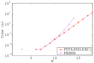
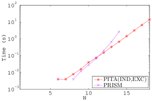
In order to investigate the relative performances of PITA(IND,EXC) and PRISM, we computed the execution time of queries to hmm/1 for increasing lengths of the output sequence. Sequences used in Figure 1(a) are randomly generated, while those in Figure 1(b) are repetitions of the sequence a,c,g,t. (Version 2.0 of Prism was used in all the experiments.) In both cases, the costs for both algorithms grow exponentially. Times for both systems are close for $N$ up to 11; however beyond $N=12$, PITA(IND,EXC) begins to scale somewhat better than Prism, answering queries through $N=18$ while Prism can answer queries only through $N=14$. Beyond those numbers, both systems throw memory errors.

(a) PITA(IND,EXC) and PRISM on random sequences.

(b) PITA(IND,EXC) and PRISM on repeated sequences.

Figure 1: Times for computing $P(hmm(<seq>))$ as a function of sequence length. Missing points at the beginning of the $X$-axis correspond to a time smaller than $10^{-6}$ seconds, missing points at the end of the $X$-axis correspond to a memory error. The experiments were performed on a Core 2 Duo E6550 (2333 MHz) processor.

[Christiansen and Gallagher (2009)] proposed a technique for speeding up query answering by removing non-discriminating arguments. These are arguments that play no role in determining the control flow of a logic program with respect to goals satisfying given mode and sharing restrictions. The computation trees of the resulting program are isomorphic to those of the original program and the results of the original program can be reconstructed from a trace of the transformed program. The authors show that the removal of non-discriminating arguments is very useful with tabling because the calls to a tabled predicate differing only in the non-discriminating arguments will merge into a single table that is much smaller and has a higher chance of reuse. After removing non-discriminating arguments, the HMM program above becomes

hmm(O)$\leftarrow$ hmm(q1,O).

hmm(end,[]).

hmm(Q,[L$|$O])$\leftarrow$ Q $\backslash=$ end, succ(Q,Q1,S0),out(Q,L,S0),hmm(Q1,O).

plus the clauses defining $succ/2$ and $out/2$.

(a) PITA(IND,EXC) and PRISM on random sequences.

(b) PITA(IND,EXC) and PRISM on repeated sequences.

Figure 2: Times for computing $P(hmm(<seq>)$ as a function of sequence length (reduced program with non-discriminating arguments removed). The experiments were performed on a Core 2 Duo E6550 (2333 MHz) processor.

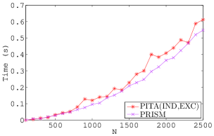
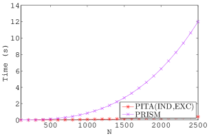
Figures 2(a) and 2(b) show the computation time for PITA(IND,EXC) and PRISM on the reduced HMM program as a function of the sequence length for randomly generated and repeating sequences. For random sequences, PITA(IND,EXC) and Prism are competitive, with Prism slightly faster; however for the repeating sequences PITA(IND,EXC) is much faster, and in fact scales well up to input sequences of length ${\mathcal{}O}(10^{5})$. The reason for the scalability of PITA(IND,EXC) on repeated sequences is apparently due to XSB’s use of trie-based tables, which allows good indexing and space sharing for repeating subsequences. The tabling of Prism, which is based on hash tables, loses discrimination in this case.

Computing the Viterbi Path.

In HMMs, it is common to look for the sequence of state values that most likely gave the output sequence, also called the Viterbi path, while the probability of this sequence of states is called the Viterbi probability. This is equivalent to finding the most probable explanation for the goal.

The Viterbi path and probability are computed by PRISM with the $\mathit{viterbif}/3$ predicate but can be computed also by PITA(IND,EXC) by modifying it so that the probability data structure includes not only the highest probability of the subgoal but also the most probable explanation for the subgoal. In this case the support predicates are modified as follows:

equality(R,S,Probs,N,e([(R,S,N)],P))$\leftarrow$ nth(N,Probs,P).
or(e(E1,P1),e(_E2,P2),e(E1,P1))$\leftarrow P1>=P2,!.$
or(e(_E1,_P1),e(E2,P2),e(E2,P2)).
and(e(E1,P1),e(E2,P2),e(E3,P3))$\leftarrow$ P3 is  P1*P2,append(E1,E2,E3).
zero(e(null,0)).	one(e([],1)).	ret_prob(B,B).

In this way we obtain PITAVIT(IND), which is also sound if the exclusiveness assumption does not hold.

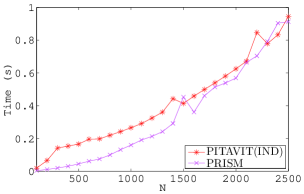
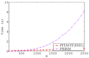
Figures 3(a) and 3(b) show times for PITAVIT(IND) and PRISM to compute Viterbi paths and probabilities on the reduced HMM program. PITAVIT(IND) is slower than PRISM for short random sequences and roughly the same on long sequences. On repeated sequences it is much more scalable.

(a) PITAVIT(IND) and PRISM on random sequences.

(b) PITAVIT(IND) and PRISM on repeated sequences.

Figure 3: Times for computing the Viterbi path and probability of $hmm(<seq>)$ as a function of sequence length (reduced program with non-discriminating arguments removed). The timings were taken on an Intel Core i5 (2.53 GHz) processor.

Counting Explanations PITA(IND,EXC) can be used to count explanations for goals with a slight modification when explanations for different goals are not incompatible. To obtain PITA(COUNT), the only auxiliary predicate to be modified is $equality/3$: $\begin{array}[]{ll}equality(\_Probs,\_N,1).\end{array}$

7 Application to Possibilistic Logic Programming

PITA also can be used to perform inference in Possibilistic Logic Programming where a program is composed only of clauses of the form $H:\alpha\leftarrow B_{1},\ldots,B_{n}$ which we interpret as possibilistic clauses of the form $(H\leftarrow B_{1},\ldots,B_{n},\alpha)$. For space reasons we do not discuss negation here, however the publicly available version of PITA computes possibilistic programs that are left-to-right dynamically stratified (Section 4) according to the semantics of [Bauters et al. (2010)].

The transformation $PITA^{P}$ used for the PRISM optimization can be used unchanged provided the support predicates are defined as

equality([P,_P0],_N,P).
or(A,B,C)$\leftarrow$ C is max(A,B).		and(A,B,C)$\leftarrow$ C is min(A,B).
zero(0.0).	one(1.0).	ret_prob(P,P).

We obtain in this way PITA(POSS). The input list of the $equality/3$ predicate contains two numbers because we used the same preprocessing code as for LPADs. Specializing the transformation for possibilistic logic programs would remove the need for the $equality/3$ predicate.

To experiment with PITA(POSS), we consider the networks of biological concepts of [De Raedt et al. (2007)] and the definition of path/2 of Example 2. In these networks the nodes encode biological entities and the edges conceptual relations among them. In each program the edges are associated to a real number. The programs have been sampled from a very large graph and contain 200, 400, $\ldots$, 10000 edges. Sampling was repeated ten times, to obtain ten series of programs of increasing size. In each program we query the possibility that the two genes HGNC_620 and HGNC_983 are related.

We use PITA(COUNT) to compute the number of explanations for the query in the first series of programs. In this problem, an explanation is a path from source to target that does not contain loops. In fact, paths with loops are subsumed by paths without loops so they do not contribute to the overall probability. Table 1 shows the number of paths for the networks in series 1 for which the computation terminated in 24 hours.

Table 1: Number of paths.

Edges	200	400	600	800	1000	1200
Explanations	10	42	380	1,280	3,480	612,140

As you can see, the number of paths grows very fast.

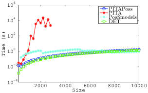
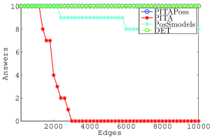
Figure 4(a) shows the average over the ten series of the execution time for computing the possibility of path(’HGNC_620’,’HGNC_983’) as a function of the number of edges. Figure 4(b) shows the number of graphs solved for each graph size. These figures also contain data for PITA(PROB), for the equivalent deterministic program (i.e. computing whether there is a path between nodes) and for the system posSmodels [Nicolas et al. (2006)]. As these figures show, computing the possibility is much easier than computing the general probability, which must solve the disjoint sum problem to obtain answers. With respect to the posSmodels system, PITA(POSS) is faster for smaller graphs and slower for larger ones, but the averages of posSmodels have been computed on less graphs since on some it gave a lack of memory error.

(a) Average time.

(b) Number of solved graphs.

Figure 4: Results of the experiments on the biological networks. The experiments were performed on an Intel Core 2 Duo E6550 (2333 MHz) processor and 4 GB of RAM.

8 Conclusions

We have shown how the probabilsitic inference system PITA can be easily adapted for different settings. In particular, we have considered programs that respect the independence and exclusion assumptions that are required by PRISM and show how PITA can be modified to exploit these assumption. Preliminary results show the algorithm to be faster than PRISM for complex queries to a naive encoding of an HMM, while the performance on an optimized encoding depend on the input data. Moreover, PITA can be used also for computing the Viterbi path, i.e., the most probable explanation for a goal. Finally, we have shown how PITA can be modified to perform inference on Possibilistic Logic Programs.

PITA is a supported package in version 3.3 of XSB, and handles programs that include both negation and function symbols. Because PITA consists of a program transformation plus library functions that implement an API for answer subsumption, the approaches of general PLP, restricted PLP and Possibilistic Logic Programming can be combined within a single program. Thus, if it is known that, say, predicates in a given module satisfy independence and exclusiveness assumptions, the module can use PITA(IND,EXC) and avoid the expense of BDD maintenance. Furthermore, simple modifications to PITA would allow the use of general vs. restricted PLP to be decided on a predicate basis, possibly supported in the future by an optimizing compiler that could check exclusiveness of clauses, and independence of literals within the body of a clause. This approach is not only general, but portable. For Prologs that implement tabling, the additional effort needed for answer subsumption is relatively small so that implementations of PITA need not be restricted to XSB.

Finally, we believe that the techniques presented can be applied also to Soft Constraint Logic Programming (SCLP) [Bistarelli and Rossi (2001)], as advocated in [Bistarelli et al. (2007)]. In this case, PITA’s API to answer subsumption would interface with a constraint handling system rather than to BDDs or to simple Prolog predicates. In fact, PITA, PITA(IND,EXC) and PITA(POSS) can be as seen as implementing SCLP over the semirings $\langle\mathcal{P},\vee,\wedge,\mathit{false},true\rangle$, $\langle[0,1],+,\times,0,1\rangle$ and $\langle[0,1],\max,\min,0,1\rangle$ respectively, where $\mathcal{P}$ is the set of propositional formulas built over a fixed and finite set of propositions.

Acknowledgements The authors thank Henning Christiansen for his help in validating the experimental results that use removal of non-discriminating arguments. The work of the first author has been partially supported by the Camera di Commercio, Industria, Artigianato e Agricoltura di Ferrara, under the project titled ”Image Processing and Artificial Vision for Image Classifications in Industrial Applications”.

References

- Baral et al. (2009) Baral, C., Gelfond, M., and Rushton, J. N. 2009. Probabilistic reasoning with answer sets. Theor. Pract. of Log. Prog. 9, 1, 57–144.
- Bauters et al. (2010) Bauters, L., Schockaert, S., De Cock, M., and Vermeir, D. 2010. Possibilistic answer set programming revisited. In Conference on Uncertainty in Artificial Intelligence. AUAI Press.
- Bistarelli et al. (2007) Bistarelli, S., Montanari, U., Rossi, F., and Santini, F. 2007. Modelling multicast QoS routing by using best-tree search in and-or graphs and soft constraint logic programming. Electr. Notes Theor. Comput. Sci. 190, 3, 111–127.
- Bistarelli and Rossi (2001) Bistarelli, S. and Rossi, F. 2001. Semiring-based contstraint logic programming: syntax and semantics. ACM Trans. Program. Lang. Syst. 23, 1, 1–29.
- Christiansen and Gallagher (2009) Christiansen, H. and Gallagher, J. P. 2009. Non-discriminating arguments and their uses. In International Conference on Logic Programming. LNCS, vol. 5649. Springer, 55–69.
- Dantsin (1991) Dantsin, E. 1991. Probabilistic logic programs and their semantics. In Russian Conference on Logic Programming. LNCS, vol. 592. Springer, 152–164.
- (7) De Raedt, L., Demoen, B., Fierens, D., Gutmann, B., Janssens, G., Kimmig, A., Landwehr, N., Mantadelis, T., Meert, W., Rocha, R., Santos Costa, V., Thon, I., and Vennekens, J. Towards digesting the alphabet-soup of statistical relational learning. In NIPS2008 Workshop on Probabilistic Programming.
- De Raedt et al. (2007) De Raedt, L., Kimmig, A., and Toivonen, H. 2007. ProbLog: A probabilistic Prolog and its application in link discovery. In Internation Joint Conference on Artificial Intelligence. 2462–2467.
- Dubois et al. (1991) Dubois, D., Lang, J., and Prade, H. 1991. Towards possibilistic logic programming. In International Conference on Logic Programming. 581–595.
- Dubois et al. (1994) Dubois, D., Lang, J., and Prade, H. 1994. Possibilistic logic. In Handbook of logic in artificial intelligence and logic programming,vol. 3, D. M. Gabbay, C. J. Hogger, and J. A. Robinson, Eds. Oxford University Press, 439–514.
- Dubois and Prade (2004) Dubois, D. and Prade, H. 2004. Possibilistic logic: a retrospective and prospective view. Fuzzy Sets Syst. 144, 1, 3–23.
- Kersting and De Raedt (2000) Kersting, K. and De Raedt, L. 2000. Bayesian logic programs. In Inductive Logic Programming, Work in Progress Track.
- Kimmig et al. (2008) Kimmig, A., Costa, V. S., Rocha, R., Demoen, B., and Raedt, L. D. 2008. On the efficient execution of problog programs. In International Conference on Logic Programming. LNCS, vol. 5366. Springer, 175–189.
- Meert et al. (2009) Meert, W., Struyf, J., and Blockeel, H. 2009. CP-Logic theory inference with contextual variable elimination and comparison to BDD based inference methods. In International Conference on Inductive Logic Programming. LNCS, vol. 5989. Springer, 96–109.
- Nicolas et al. (2006) Nicolas, P., Garcia, L., Stéphan, I., and Lefèvre, C. 2006. Possibilistic uncertainty handling for answer set programming. Ann. Math. Artif. Intell. 47, 1-2, 139–181.
- Nieves et al. (2007) Nieves, J. C., Osorio, M., and Cortés, U. 2007. Semantics for possibilistic disjunctive programs. In International Conference on Logic Programming and Nonmonotonic Reasoning. LNCS, vol. 4483. Springer, 315–320.
- Osorio and Nieves (2009) Osorio, M. and Nieves, J. C. 2009. Possibilistic well-founded semantics. In Mexican International Conference on Artificial Intelligence. LNCS, vol. 5845. Springer, 15–26.
- Poole (1993) Poole, D. 1993. Logic programming, abduction and probability - a top-down anytime algorithm for estimating prior and posterior probabilities. New Gener. Comput. 11, 3, 377–400.
- Poole (1997) Poole, D. 1997. The Independent Choice Logic for modelling multiple agents under uncertainty. Artif. Intell. 94, 1–2, 7–56.
- Poole (2000) Poole, D. 2000. Abducing through negation as failure: stable models within the independent choice logic. J. Log. Program. 44, 1-3, 5–35.
- Riguzzi (2007) Riguzzi, F. 2007. A top down interpreter for LPAD and CP-logic. In Congress of the Italian Association for Artificial Intelligence. LNAI, vol. 4733. Springer, 109–120.
- Riguzzi (2008) Riguzzi, F. 2008. Inference with logic programs with annotated disjunctions under the well founded semantics. In International Conference on Logic Programming. LNCS, vol. 5366. Springer, 667–771.
- Riguzzi (2009) Riguzzi, F. 2009. Extended semantics and inference for the Independent Choice Logic. Logic J. of the IGPL 17, 6, 589–629.
- Riguzzi (2010) Riguzzi, F. 2010. SLGAD resolution for inference on Logic Programs with Annotated Disjunctions. Fundam. Inform. 102, 3-4, 429–466.
- Riguzzi and Swift (2010a) Riguzzi, F. and Swift, T. 2010a. An extended semantics for logic programs with annotated disjunctions and its efficient implementation. In Italian Conference on Computational Logic. CEUR Workshop Proceedings, vol. 598. Sun SITE Central Europe.
- Riguzzi and Swift (2010b) Riguzzi, F. and Swift, T. 2010b. Tabling and Answer Subsumption for Reasoning on Logic Programs with Annotated Disjunctions. In Technical Communications of the International Conference on Logic Programming. LIPIcs, vol. 7. Schloss Dagstuhl–Leibniz-Zentrum fuer Informatik, 162–171.
- Santos Costa et al. (2003) Santos Costa, V., Page, D., Qazi, M., and Cussens, J. 2003. CLP(): Constraint logic programming for probabilistic knowledge. In Conference on Uncertainty in Artificial Intelligence. Morgan Kaufmann.
- Sato (1995) Sato, T. 1995. A statistical learning method for logic programs with distribution semantics. In International Conference on Logic Programming. MIT Press, 715–729.
- Sato et al. (2010) Sato, T., Zhou, N.-F., Kameya, Y., and Izumi, Y. 2010. PRISM User s Manual (Version 2.0). http://sato-www.cs.titech.ac.jp/prism/download/prism20.pdf.
- Swift (1999) Swift, T. 1999. Tabling for non-monotonic programming. Ann. Math. Artif. Intell. 25, 3-4, 201–240.
- Vennekens and Verbaeten (2003) Vennekens, J. and Verbaeten, S. 2003. Logic programs with annotated disjunctions. Tech. Rep. CW386, K. U. Leuven.
- Vennekens et al. (2004) Vennekens, J., Verbaeten, S., and Bruynooghe, M. 2004. Logic programs with annotated disjunctions. In International Conference on Logic Programming. LNCS, vol. 3131. Springer, 195–209.
- Zhou (2011) Zhou, N.-F. 2011. The language features and architecture of B-Prolog. CoRR abs/1103.0812.