Non-Gaussianity from the hybrid potential

Abstract

We study the hybrid inflationary potential in a regime where the defect field is light, and more than 60 e-folds of accelerated expansion occur after the symmetry breaking transition. Using analytic and numerical techniques, we then identify parameter values within this regime for which the statistics of the primordial curvature perturbation are significantly non-Gaussian. Focusing on this range of parameters, we provide a specific example which leads to an observationally consistent power spectrum, and a level of non-Gaussianity within current WMAP bounds and in reach of the Planck satellite. An interesting feature of this example is that the initial conditions at horizon crossing appear quite natural.

I Introduction

An inflationary epoch is the most promising model for the origin of large-scale structure in the universe inflation (for reviews see reviews ), naturally accounting for current observations which indicate that the universe’s structure originated from near-scale invariant and almost Gaussian fluctuations observations ; wmap . The small deviations from scale-invariance and Gaussianity are key probes of inflation, allowing competing models to be distinguished from one another by present and future observations.

In canonical, single field inflation, the curvature perturbation produced at horizon crossing is extremely close to Gaussian, and is conserved through the entirety of the subsequent evolution Maldacena:2002vr ; Bardeen ; Lyth ; zetaConv . On the other hand, when more than one field is light at horizon crossing, isocurvature modes are produced, which later can source an additional contribution to the curvature perturbation. This can cause the curvature perturbation to become sufficiently non-Gaussian for this signal to be detected by future observations, or the model constrained by present ones. The current WMAP constraints on the $f_{\rm NL}$ parameter, which measures the deviation of the three–point correlation function from zero, is $-10<f_{\rm NL}<74$ at $95\%$ confidence level, but $f_{\rm NL}\approx 32\pm 21$ at the $68\%$ level wmap . Though premature, it is tempting to consider these numbers as a ‘tentative hint’ of a non-Gaussian signal. The recently launched PLANCK satellite, will help resolve the issue. In the absence of a detection it is expected to give the constraint $|f_{\rm NL}|<5$.

With these issues in mind, considerable effort has been invested in developing methods to calculate how non-Gaussianity evolves on super-horizon scales during inflation, Lyth:2005fi ; Vernizzi:2006ve ; otherMethods , into identifying the features an inflationary potential must possess and the initial conditions required, to lead to a ‘large’ non-Gaussianity ($f_{\rm NL}>1$) largeNG1 ; largeNG2 ; Kim:2010ud ; Elliston:2011dr . Many scenarios have also been studied in which the generation of non-Gaussianity occurs due to post inflationary effects, such as in curvaton curv , preheating preh , modulated (p)reheating mod , and models with an inhomogenious end of inflation inHom1 ; inhom2 (see Ref. Alabidi:2010ba for connections between these three scenarios).

Of particular interest are effects which occur for inflationary potentials which are well motivated from a particle physics perspective. The hybrid potential is one such example, and moreover is one of the most widely studied potentials in the literature. First introduced as an inflationary model by Linde Linde:1993cn , it is a two-field potential of the form

$$V(\phi,\chi)=\frac{1}{2}m^{2}\phi^{2}+\frac{1}{2}g^{2}\phi^{2}\chi^{2}+\frac{\lambda}{4}(\chi^{2}-v^{2})^{2}\,.$$ (1)

As a quantum field theory, this is attractive because it is renormalisable and does not require unnatural cancellation of radiative corrections. In fact, potentials of this type are common in supersymmetric models SUSY .

In this paper we will investigate the hybrid potential (1) using a different choice of parameters from the original proposal. We find that this leads to a viable cosmological model, with perturbations that are compatible with current observations and level of non-Gaussianity that would be observable with the Planck satellite.

II Original Hybrid Inflation

In the original version of the scenario Linde:1993cn the $\phi$ field plays the role of the inflaton. Initially, $\phi$ has a value larger than the ‘critical’ value, $\phi>\phi_{\rm crit}\equiv\sqrt{\lambda}v/g$, but still below the Planck scale $\phi\ll m_{\rm pl}=(8\pi G)^{-1/2}$. The latter requires $\lambda v^{2}<g^{2}m_{\rm pl}^{2}$. The field $\phi$ then rolls down the potential towards smaller values until it reaches $\phi_{\rm crit}$, at which point $\chi$ becomes non-zero and inflation ends.

We can generally consider a multi-field model with scalar fields $\varphi^{\alpha}$ labelled by an integer $\alpha$. In the case of the hybrid model, the fields are $\varphi_{1}=\phi$ and $\varphi_{2}=\chi$. Defining the slow-roll parameters,

$$\epsilon_{\alpha}=\frac{m_{\rm pl}^{2}}{2}\left(\frac{V_{,\alpha}}{V}\right)^{2}\,,$$ (2)

and

$$\eta_{\alpha\beta}=m_{\rm pl}^{2}\frac{V_{,\alpha\beta}}{V}\,,$$ (3)

the universe inflates when $\epsilon\equiv\sum_{\alpha}\epsilon_{\alpha}<1$ and when $\epsilon\ll 1$ the fields satisfy the ‘slow-roll’ equations of motion

$$\frac{d\varphi^{\alpha}}{dN}=-\sqrt{2\epsilon_{\alpha}}m_{\rm pl}\,.$$ (4)

The standard hybrid model assumes that the potential (1) is dominated by the constant term during inflation, and this requires $\lambda v^{4}>m^{2}m_{\rm pl}^{2}$. The parameters are also chosen such that when $\phi$ reaches $\phi_{\rm crit}$, $\chi$ rapidly grows and reaches the global minimum at $\chi=\pm v$ in less than an e-fold Copeland:2002ku , thus ending inflation. This requires that the potential is steep enough in the $\chi$ direction to avoid further inflation, or more precisely $v<m_{\rm pl}$. Also, $\phi$ must pass through $\phi_{\rm crit}$ fast enough that $\chi$ remains light for less than an e-fold. Utilising Eq. (4) and (2) and linearising about $\phi_{\rm crit}$ such that $\Delta\phi=\phi-\phi_{\rm crit}$, $\Delta N=\sqrt{\epsilon_{\phi_{\rm crit}}}\Delta\phi$, and $m^{2}_{\chi}=2g^{2}\phi_{\rm crit}\Delta\phi$. One finds that $\chi$ is light for $N\approx\lambda v^{6}/(m^{2}m_{\rm pl}^{4})$, and hence this combination of parameters must be less than unity. To summarise, therefore, the original scenario requires the parameter choices

$$\lambda v^{2} < g^{2}m_{\rm pl}^{2},$$

$$\lambda v^{4} > m^{2}m_{\rm pl}^{2},$$

$$v < m_{\rm pl},$$

$$\lambda v^{6} < m^{2}m_{\rm pl}^{4}.$$ (5)

It is important to realise, however, that these constraints are not all necessarily required for a viable cosmological model. They simply correspond to the specific physical scenario assumed in the original papers. Despite having many appealing features, this original scenario suffers from two important issues. First, the phase transition generates a network of domains where different choices of vacuum have been made. The domains are separated by domain walls, which are incompatible with the observable universe. This issue can be overcome by using a multi-component $\chi$ field, and possibly coupling it to a gauge field to eliminate Goldstone bosons, but this complicates the model significantly. Second, the scenario predicts a blue spectral index ($n_{s}>1$). This is because for inflation driven solely by the $\phi$ field, $n_{\rm s}=1-6\epsilon^{*}_{\phi}+2\eta^{*}_{\phi\phi}$ (where ^∗ labels the time at which observational wavelengths became greater than the cosmological horizon roughly $60$ e-folds before the end of inflation), and for the parameter choices discussed above, $\eta^{*}_{\phi\phi}$ is positive and satisfies $\eta_{\phi\phi}^{*}\gg\epsilon^{*}_{\phi}$. This is in conflict with WMAP and baryon acoustic oscillations measurements which give $n_{s}=0.968\pm 0.012$ with $68\%$ confidence level wmap .

III Hybrid inflation with two light fields

Given the motivation for the form of potential (1), it is interesting to study its consequences outside of the parameter ranges (II) which lead to the original scenario. For example, considerable interest has been devoted to parameter choices which make both fields light (see for example Randall:1996ip ; GarciaBellido:1996qt ), and there have been a number of investigations into the consequences of this situation, such as the resultant non-Gaussianity barnaby . If the waterfall field is light at the symmetry breaking transition for more than an e-fold, however, the amplitude of density perturbations on scales associated with this transition is in tension with primordial black hole constraints GarciaBellido:1996qt .

Recently, it has been noted by Clesse Clesse:2010iz that this conclusion does not apply if the waterfall field is light but more than $60$ e-folds of inflation occur after the phase transition. This is because any black holes produced are diluted by the expansion, and moreover, this also solves the defect problem, as defects are pushed onto scales larger than the present day observable universe. Clesse considered a parameter range identical to the original hybrid scenario, except that he choose parameters such that $\phi$ stays sufficiently close to $\phi_{\rm crit}$ for $\chi$ to be light for more than $60$ e-folds, requiring $\lambda v^{6}\gg 60m^{2}m_{\rm pl}^{2}$. In this minimal adjustment to the original scenario, both fields still move sub-Planckian distances, but the velocity of the $\chi$ field is much greater than the $\phi$ field for the entire evolution. This implies that $n_{s}=1-6\epsilon_{\chi}+2\eta_{\chi\chi}$ and because the model is still vacuum dominated and $\eta_{\chi}$ is negative (because inflation occurs after the transition where $\chi$ has a negative mass), a red spectral index results. The final issue with the original scenario is therefore resolved.

Clesse’s scenario does not lead to observable levels of non-Gaussianity. In this paper we show that there are other parameter choices which lead to perturbations that are compatible with observations but are significantly non-Gaussian.

IV The $\mathbf{\delta}$N formalism.

To calculate the level of non-Gaussianity as well as the amplitude of the power spectrum and the spectral index, we will employ the $\delta N$ formalismStarobinsky:1986fxa ; Sasaki:1995aw ; Lyth:2005fi , implemented with numerical and analytic techniques.

The $\delta N$ formalism, assumes the separate universe approximation, in which points in the universe separated by more than a horizon size evolve like a ‘separate universe’, the dynamics following from the local energy density and pressure, and obeying the field equations of a Friedmann-Robertson-Walker (FRW) universe (see for example Lyth ; Wands:2000dp ). The $\delta N$ formalism then notes that the uniform density curvature perturbation between two such points, $\zeta$, is given by the difference in e-folds of expansion between them, from some initial shared flat hypersurface labelled $*$, to some final shared hypersurface of uniform density labelled $f$,

$$\zeta=\delta N^{f}_{*}.$$ (6)

We use $*$ to label the flat hypersurface, since in order to make observational predictions for an inflationary model, this surface must be defined at the time when obervable scales exited the cosmological horizon. Moreover, the final hypersurface $f$ must be taken at some much later time when the dynamics are adiabatic and $\zeta$ is conserved. This can happen, for example, long after inflation ends, when the dynamics are dominated by a single fluid.

When slow-roll is a good approximation at horizon exit, $\zeta$ is completely determined by the field perturbations $\delta\varphi^{\alpha}_{*}$ at that time,

$$\zeta=\delta N_{*}^{f}(\delta\varphi^{\alpha}_{*}).$$ (7)

The field perturbations are extremely close to Gaussian Gaussian , and if their amplitude is sufficiently small, the statistics of the curvature perturbation can be determined in a simple manner by Taylor expanding

$$\delta N^{f}_{*}\approx\frac{\partial N^{f}_{*}(\phi_{*},\chi_{*})}{\partial\varphi^{\alpha}_{*}}\delta\varphi^{\alpha}_{*}+\frac{1}{2}\frac{\partial^{2}N^{f}_{*}}{\partial\varphi^{\alpha}_{*}\varphi^{\beta}_{*}}\delta\varphi^{\alpha}_{*}\delta\varphi^{\beta}_{*}\,,$$ (8)

where here and from here on we employ the summation convention, and subsequently we will employ the notation in common use, $N_{\alpha}={\partial N^{f}_{*}(\phi_{*},\chi_{*})}/{\partial\varphi^{\alpha}_{*}}$.

One then finds that the amplitude of the power spectrum is given by

$$A_{\zeta}^{2}=N_{\alpha}N_{\alpha}\frac{H_{*}^{2}}{4\pi^{2}}\,,$$ (9)

the spectral index $n_{s}$ by Sasaki:1995aw

$$n_{s}=1-2\epsilon_{*}+\frac{2}{H_{*}}\frac{\dot{\varphi}^{\alpha}_{*}N_{\beta}N_{\alpha\beta}}{N_{\alpha}N_{\alpha}}\,,$$ (10)

which generalises the single field expression we employed earlier, and the amplitude of the reduced bispectrum by Lyth:2005fi

$$f_{\rm NL}=\frac{5}{6}\frac{N_{\alpha}N_{\beta}N_{\alpha\beta}}{(N_{\alpha}N_{\alpha})^{2}}\,.$$ (11)

V Analytic estimates

In the end we will analyse the model using numerical methods, but to identify suitable parameter ranges, let us first use analytic approximations to model the behaviour of the model. One particular case in which analytic calculations are possible is when the potential is separable,

$$V(\phi,\chi)=V_{\phi}(\phi)+V_{\chi}(\chi).$$

Of course, the hybrid potential Eq. (1) is not separable, but this should still be a reasonable approximation if the non-separable term $g^{2}\phi^{2}\chi^{2}$ is sub-dominant to the other terms. We will therefore use this approximation, and later check its validity using full numerical simulations.

For separable potentials, there exist analytic expressions for the derivatives of $N$ Vernizzi:2006ve ; GarciaBellido:1995qq . The starting point for these formulae are the slow-roll equations of motion Eq. (4). It follows that

$$N=\int^{f}_{*}d\phi\frac{-V(\phi,\chi)}{m_{\rm pl}^{2}V_{,\phi}}=\int^{f}_{*}d\phi\frac{-V_{\phi}}{m_{\rm pl}^{2}V_{,\phi}}+\int^{f}_{*}d\chi\frac{-V_{\chi}}{m_{\rm pl}^{2}V_{,\chi}}\,.$$ (12)

Therefore, for example,

$$N_{,\chi}=\left.\frac{V_{\chi}}{m_{\rm pl}^{2}V_{,\chi}}\right|_{*}-\left.\frac{V_{\chi}}{m_{\rm pl}^{2}V_{,\chi}}\right|_{*}\frac{\partial\phi^{f}}{\partial\phi_{*}}\,.$$ (13)

The complexity of the calculation then reduces to determining the partial derivative of the final field value on a constant energy density hypersurface with respect to the initial field value. However, when the dynamics become adiabatic during inflation, this derivative tends to zero. Therefore, one usually finds that $N_{\chi}=V_{\chi}/(m_{\rm pl}^{2}V_{,\chi}|_{*})$. The second derivatives of $N$ then follow by simple differentiation.

One known mechanism which gives rise to a large non-Gaussianity in multiple field inflation is for one of the fields to be very close to a maximum of its self-interaction potential at the time of horizon crossing Kim:2010ud ; Elliston:2011dr , and for the magnitude of its tachyonic mass–squared to be much greater than the vacuum energy at this hilltop. In this region the $\chi$ part of the potential can be approximated by $V_{\chi}=V_{0}-1/2m_{\chi}^{2}\chi^{2}$, and the condition required is that $m_{\chi}^{2}m_{\rm pl}^{2}\gg V_{0}$ Kim:2010ud . Of course the field must also be light at horizon crossing, and hence $m_{\chi}^{2}<H^{2}$, but this condition can be simultaneously satisfied assuming the potential is not vacuum dominated, and that another field contributes significantly to the total energy density.

Following Ref. Kim:2010ud we can understand this condition by considering that when $m_{\chi}^{2}\chi^{2}<V_{0}$, $N_{\chi}\approx-V_{0}/(m_{\rm pl}^{2}m_{\chi}^{2}\chi_{*})$, which becomes large in the limit that $\chi_{*}\rightarrow 0$. In this limit, the contribution to $\delta N$ from the $\chi$ field likely dominates over all other contributions, and moreover $N_{\chi\chi}\approx V_{0}/(m_{\rm pl}^{2}m_{\chi}^{2}\chi_{*}^{2})$, and $f_{\rm NL}\approx(5m_{\rm pl}^{2}m_{\chi}^{2})/(6V_{0})$.

For the hybrid potential well after the symmetry breaking transition, the shape of the potential is exactly of the form discussed above, with the non-separable term sub-dominant. In that case, $V_{0}=\lambda v^{4}/4$, $m_{\chi}^{2}=\lambda v^{2}$ and hence for this regime we expect

$$f_{\rm NL}\approx\frac{10}{3}\frac{m_{\rm pl}^{2}}{v^{2}}\,,$$ (14)

assuming that $\chi_{*}$ is sufficiently small.

In principle, therefore, for $v<m_{\rm pl}$ it is possible for this hybrid potential to give rise to a large positive non-Gaussianity. The additional constraint that the $\chi$ field be light, however, introduces the restriction that $1/2m_{\phi}^{2}\phi_{*}^{2}\gg V_{0}=\lambda v^{4}/4$, and the $\phi$ part of the potential dominates the energy density. This implies we must move beyond the original parameter choices and consider large field values of $\phi$ in order that sufficient inflation occurs. This in turn implies that $\phi_{\rm crit}\geq 16m_{\rm pl}$, where equality leads to roughly $60$ e-folds after the transition. Hence $\phi*\approx 16m_{\rm pl}$. In this case $N_{\phi}=\phi_{*}/(2m_{\rm pl}^{2})$, and the condition that the $\chi$ field sources the dominant contribution to $\delta N$, $|N_{\chi}|>|N_{\phi}|$, implies that $v^{2}>32\chi_{*}m_{\rm pl}$. We arrive at the curious situation in which the $\phi$ field sources inflation, while the contribution due to the $\chi$ field dominates $\zeta$, and can be extremely non-Gaussian. This can be summarised by the following requirements on the parameters

$$\lambda v^{2} \gg g^{2}m_{\rm pl}^{2},$$

$$m^{2}\phi^{*2} \gg \lambda v^{4},$$

$$v < m_{\rm pl},$$

$$\phi_{*} \approx 16m_{\rm pl},$$

$$\chi_{*} \lesssim 0.03v^{2}/m_{\rm pl}$$ (15)

On the other hand, consideration of Eq. (10) implies that the spectral index is generically red tilted and close to scale invariant, as will be confirmed by the full numerical simulations which follow.

Guidance from analytic arguments, therefore, appears to lead to a large non-Gaussianity in the following scenario. Long before the last $60$ e-folds of inflation, $\phi$ begins its evolution with $\phi>\phi_{\rm crit}$, and some value of $\chi$. Since the mass of $\chi$ is initially positive it will evolve towards its minimum at $\chi=0$ as $\phi$ evolves towards $\phi_{\rm crit}$. Assuming the classical evolution of $\chi$ reaches $\chi=0$ before $\phi$ reaches $\phi_{\rm crit}$, then at this time the value of $\chi$ will be dominated by its quantum diffusion during the period before the transition for which it was light. After the transition for the parameter choices discussed, more than $60$ e-folds of inflation occur and $\chi$ is still light when $\phi=16m_{\rm pl}$ roughly $60$ e-folds before the end of inflation. Its vev at this time will then likely still be close to $\chi=0$. The $\chi$ field will only roll significantly when $\chi$ becomes heavy. If this occurs before $\phi$ evolves to its minimum, it will roll during the slow-roll inflationary phase, otherwise $\phi$ will begin oscillating and begin to decay into radiation before $\chi$ begins to roll. In the later case $\chi$ will perhaps source an extremely short secondary inflationary phase as it rolls. It is clear, however, that Eq. (14) will remain at best a rough estimate. This is why we employ numerical simulations in our study.

For completeness we note that when $\chi_{*}$ becomes larger and Eq. (14) becomes obsolete, it is still possible to find an analytic estimate for the asymptotic value of $f_{\rm NL}$. At $\chi_{*}\sim v^{2}/m_{\rm pl}$, we reach a regime where $|N_{\phi}|>|N_{\chi}|$. If the numerator of Eq. (11) is still dominated by $\chi$, we find

$$f_{\rm NL}=\frac{5}{6}\frac{N_{\chi}^{2}N_{\chi\chi}}{N_{\phi}^{4}}\approx\frac{v^{6}}{m_{\rm pl}^{2}\chi_{*}^{4}},$$ (16)

indicating that $f_{\rm NL}$ drops sharply. At even larger values of $\chi_{*}$, we find $N_{\phi\phi}>N_{\chi\chi}$, which implies $f_{\rm NL}=5N_{\phi\phi}/(6N_{\phi}^{2})$. Using $N_{\phi}=\phi_{*}/2m_{\rm pl}^{2}$ and $N_{\phi\phi}=1/2m_{\rm pl}^{2}$, we obtain

$$f_{\rm NL}=\frac{5m_{\rm pl}^{2}}{3\phi_{*}^{2}}\approx 0.007.$$ (17)

Hence, we should find a smooth but clear transition from the significant non-Gaussianity predicted by Eq. (14) to practically Gaussian single-field behaviour (17) at around $\chi_{*}\approx 0.03v^{2}/m_{\rm pl}$.

VI Initial conditions

The scenario discussed above requires a small initial value for the waterfall field, $\chi_{*}\ll v^{2}/m_{\rm pl}$, at $\phi=\phi_{\rm crit}$. In this section we discuss the naturalness of this condition. This is an instance of the ‘measure problem’ which is unresolved in general. However, we can apply some heuristic arguments.

In Section V, we outlined a plausible sequence of events in which, long before the hybrid transition, both $\phi$ and $\chi$ took large values, and the classical evolution of $\chi$ tended to zero before $\phi$ reached $\phi_{\rm crit}$. The initial values of $\phi$ and $\chi$ can be motivated by assuming a phase of eternal inflation during which the path the fields follow is dominated by quantum fluctuations, rather than classical rolling. The condition for such behaviour is that the distance moved in field space in a Hubble time, is less than a typical quantum fluctuation eternal

$$\sqrt{\dot{\phi}^{2}+\dot{\chi}^{2}}>\frac{H^{2}}{\sqrt{2\pi}}\,.$$ (18)

Using the slow roll equations of motion (4) this becomes a constraint on the field values, and defines a one dimensional surface in field space at which the dynamics becomes predominantly classical.

Beginning at this surface, therefore, one might wonder whether $\chi$ will indeed reach $\chi=0$ (according to its classical rolling) before $\phi$ reaches $\phi_{\rm crit}$. The answer to this question will be extremely parameter dependent, and will likely also depend on the position on the surface from which the fields originate. It is easy, however, to build up a rough picture of the expected behaviour. Considering cases where both $\phi$ and $\chi$ are significantly displaced from zero initially, $\chi$ will likely initially be the more massive field for the parameter choices we are focusing on (15). This is because $\chi$ feels a mass of $1/2\lambda\chi^{2}+g^{2}\phi^{2}$ in comparison with $m^{2}+g^{2}\chi^{2}$, the mass of $\phi$. Moreover, we expect $\lambda>g^{2}$, unless $v$ is much less than $m_{\rm pl}$. In the following we will assume this condition on $\lambda$ and $g$. The mass of $\phi$ would only be greater initially, therefore, if $m^{2}\gtrsim\lambda\chi_{\rm e}^{2}+g^{2}\phi_{\rm e}^{2}$ (where subscript $\rm e$ represents values on the eternal inflation surface).

Assuming that $\chi$ is indeed more massive initially, it will evolve rapidly towards $\chi=0$, while $\phi$ will remain nearly frozen. As $\chi$ decreases, there will come a time when $\lambda\chi^{2}<m^{2}$. At this point if the condition $m^{2}\gtrsim g^{2}\phi^{2}_{\rm e}$ is met then the $\chi$ field will cease to be the more massive, and its evolution will slow significantly, and it will likely not reach $\chi=0$. On the other hand, if this condition is not met we expect that $\chi$ does reach zero. The necessary condition for $\chi$ to reach zero, therefore, is that $m^{2}<g^{2}\phi^{2}_{\rm e}$, which ensures that $\chi$ is always the more massive field.

This condition is likely only very approximate, but from some limited numerical probing it appears to capture the rough behaviour of the fields. In Section VIII we will look carefully at a particular parameter choice and probe the surface defined by Eq. (18). We find a complicated picture, however this rough analysis is a useful aid.

Figure 1: The non-Gaussianity parameter $f_{\rm NL}$ as a function of $\chi_{i}$ and $v$, with other parameters given by Eq. (21). Lighter shades indicate higher $f_{\rm NL}$. High values $f_{\rm NL}\gtrsim 100$ are ruled out by WMAP, and small values $f_{\rm NL}\lesssim 1$ are likely to be unobservable.

Figure 2: The spectral index $n_{s}$ as a function of $\chi_{i}$ and $v$, with other parameters given by Eq. (21). Lighter shades indicate higher $n_{s}$. All values obtained are compatible with WMAP observations.

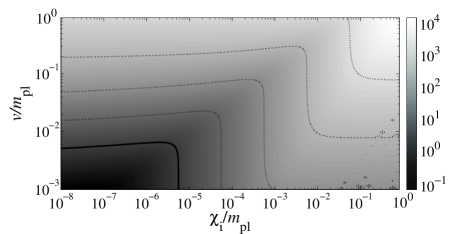
Figure 3: The ratio $\chi_{*}/H_{*}$ as a function of $\chi_{i}$ and $v$, with other parameters given by Eq. (21). Lighter shades indicate higher $\chi_{*}/H_{*}$. The thicker contour line corresponds to $\chi_{*}/H_{*}$=1. Values below this are unnatural because quantum fluctuations would generally give $\chi_{*}\gtrsim H_{*}$

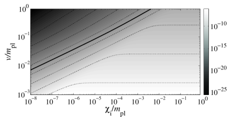
Figure 4: The dimensionless parameters $\lambda$ as a function of $\chi_{i}$ and $v$, with other parameters given by Eq. (21). Lighter shades indicate higher $\lambda$. The thicker contour line corresponds to $\lambda=10^{-14}$.

VII Numerical analysis

Having identified the interesting parameter range, we now calculate the statistics of the perturbations numerically. We evolve the full non-slow-roll equations of motion

$$\ddot{\varphi}^{\alpha}+3H\dot{\varphi}^{\alpha}+\frac{\partial V}{\partial\varphi^{\alpha}} = -\Gamma_{\alpha}\dot{\varphi}_{\alpha}\,,$$

$$\dot{\rho}_{\rm rad}+4H\rho = \Gamma_{\alpha}\dot{\varphi}_{\alpha}^{2}\,,$$ (19)

where

$$H^{2}=\frac{1}{3m_{\rm pl}^{2}}\left(\frac{1}{2}\dot{\varphi}^{\alpha}\dot{\varphi}^{\alpha}+V+\rho_{\rm rad}\right)\,,$$ (20)

and we have introduced a small decay term $\Gamma_{\alpha}$ to describe the decay of the scalar fields into radiation. As long as the decay rate is fairly slow, the produced perturbations are largely independent of it, so we do not attempt to use a realistic value but only check that our results do not depend on it.

For simplicity we reduce the number of parameters which can be varied, by fixing

$$\phi_{\rm crit} = \sqrt{1000}m_{\rm pl},$$

$$m = \sqrt{\lambda}v,$$

$$g = \sqrt{\lambda}v/\phi_{\rm crit},$$

$$\Gamma = 10^{-1}\sqrt{\lambda}v,$$ (21)

and we explore the ranges

$$10^{-3}m_{\rm pl}< v <m_{\rm pl},$$

$$10^{-6}< \chi_{\rm i}/v <1.$$ (22)

Our parameter choice effectively means that the magnitude of $H_{*}$ and of $\Gamma$ is proportional to $\sqrt{\lambda}$, and so can be scaled simply by changing the value of $\lambda$. On the other hand, since the derivatives of $N^{f}_{*}$, which enter formulae for observational quantities, are unaltered by such a scaling, changing the value of $\lambda$ leaves these derivatives unaltered. For each choice of $\chi_{\rm i}$ and $v$, we fix $\lambda$ such that the resulting amplitude $A_{\zeta}$ is in agreement with the observational requirement. The rescaling properties just discussed, however, mean that this can be done retrospectively once the derivatives of $N$ have been caculated (see below).

As discussed in Section IV, we need to calculate the amount of expansion between a flat and an equal-energy density hypersurface, $N_{*}^{f}(\phi_{*},\chi_{*})$, which we obtain by solving Eqs. (VII) for different initial values $\phi_{*}$ and $\chi_{*}$. The final hypersurface needs to be chosen in such a way that the scalar fields have decayed into radiation, so that the curvature perturbation is conserved. To find a suitable final energy density or, equivalently, final Hubble rate, we first run the code from the initial condition $\phi_{i}=\phi_{\rm crit}$ and a suitable value of $\chi_{i}$. We follow the evolution until $99.9\%$ of the energy density was in the radiation component, and use the corresponding Hubble rate $H_{f}$ to define the final hypersurface. We also record the values $\phi_{*}$ and $\chi_{*}$, which the fields take $60$ e-folds before the end of inflation. The numerical system is then re-run from initial conditions which are slightly different to the recorded $\phi_{*}$ and $\chi_{*}$, and the number of e-folds to the same final value of $H_{f}$ of the Hubble rate recorded, in such a way as to build up a finite difference approximation for the derivatives of $N_{*}^{f}(\phi_{*},\chi_{*})$.

Once we have obtained $N_{*}^{f}(\phi_{*},\chi_{*})$, we calculate the spectral index $n_{\rm s}$ and $f_{\rm NL}$ using Eqs. (10) and (11), respectively. The results in Fig. 2 show that for all the parameters we considered, the spectral index is contained in the region $0.9649\leq n_{\rm s}\leq 0.9701$. Therefore they are all compatible with the observations.

On the other hand, Fig. 1 shows that a wide range of values for $f_{\rm NL}$ are obtained, $7\times 10^{-3}\lesssim f_{\rm NL}\lesssim 5\times 10^{5}$. All parameters giving $f_{\rm NL}\gtrsim 100$ are excluded by WMAP measurements wmap , constraining the parameter space. For $\chi_{i}\lesssim 0.1v^{2}/m_{\rm pl}$, values $v\lesssim 0.07m_{\rm pl}$ are ruled out, and larger values of $\chi_{i}$ are not constrained.

Furthermore, Fig. 1 confirms the validity of the analytical arguments and estimates in Section V . To a good approximation, we can identify $\chi_{*}\approx\chi_{i}$. Our results show that as long as $\chi_{i}$ is small enough, $f_{\rm NL}$ is independent of it and decreases by one order of magnitude for a two orders of magnitude increase in $v/m_{\rm pl}$, as predicted by Eq. (14). Towards the right, at $\chi_{i}\sim 0.1v^{2}/m_{\rm pl}$, $f_{\rm NL}$ starts to fall in accordance with Eq. (16), and reaches a constant value $f_{\rm NL}\approx 0.007$ in good agreement with Eq. (17).

As mentioned above in this section, with the parametrization given in Eq. (21), we can fix the parameters of the model retrospectively, constrained by the amplitude of the power spectrum. As can be seen in Fig. 4, $10^{-6}\lesssim\lambda\lesssim 10^{-25}$.

An issue of importance is whether quantum fluctuations will affect which side of the potential the waterfall field is rolling along. This happens if the range of quantum fluctuations is greater than the distance of $\chi$ to its hilltop. It is problematic because such a scenario leads to a configuration with domain walls, which we want to avoid. For a massless scalar field, the range is given by $H_{*}/(2\pi)$. For a massive field, $H_{*}/(2\pi)$ is an upper bound. Thus, excluding parameters such that $\chi_{*}/H_{*}\leq 1$ settles the issue. As Fig. 3 shows, the excluded values are approximately $v\leq 5\times 10^{-3}m_{\rm pl}$ and $\chi_{i}<v^{2}/m_{\rm pl}$.

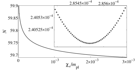
Figure 5: $N$ as a function of $\chi_{*}$ for the parameters shown in Eq. (21). The result in Section IV assume that the quadratic Taylor expansion in Eq. (8) is a good approximation. This is clearly not the case for the whole range of $\chi_{*}$, but for a range that corresponds to the values present in one comoving volume corresponding to the currently observable universe it is. This is demonstrated by the inset, which shows the data for such a range with the linear term subtracted, together with a quadratic fit.

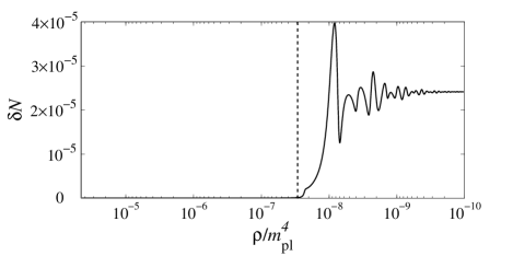
Figure 6: Comparison of two initial conditions $\chi_{i}$ and $\chi_{i}+\delta\chi_{i}$ with parameters in Eq. (21) and $\delta\chi_{i}=1.4\times 10^{-7}m_{\rm pl}$. The plotted function is the difference in $N$ as a function of enery density $\rho$, and corresponds to the curvature perturbation between points with the two different initial conditions. The vertical dashed line indicates when the waterfall field $\chi$ starts rolling down the ridge.

VIII A working example

Our results indicate that there is a fairly large window of parameters that are compatible with observations but lead to observable non-Gaussianity. We pick pick one representative example for more detailed study:

$$v = 0.2m_{\rm pl},$$

$$\lambda = 5.322\times 10^{-15},$$

$$g^{2} = 2.128\times 10^{-19},$$

$$\phi_{i} = \phi_{\rm crit},$$

$$\chi_{i} = 10^{-3}v.$$ (23)

These parameters give

$$f_{\rm NL} = 24.14,$$

$$n_{s} = 0.968.$$

Besides a value of the spectral index in the centre of the permitted observational range, these parameters give us a large, but observationally compatible, value of $f_{\rm NL}$. Indeed the value is close to the favoured WMAP value, $f_{\rm NL}\approx 20\pm 10$.

In Fig. 5, we show $N$ for a wide range of field values $\chi_{*}$. The expressions (11) and (10) for $f_{\rm NL}$ and $n_{s}$ assume quadratic Taylor expansion (8) of this function. It is clear from the figure that this assumption is not valid over the whole range shown. However, the actual range of $\chi_{i}$ present in a comoving volume corresponding to the universe observable today is smaller, roughly $\delta\chi_{i}\approx\sqrt{N/2\pi}H_{*}$, where $N\approx 60$. The inset shows this range of $\chi_{*}$, with the linear term subtracted. The remaining contribution is small and almost exactly quadratic, demonstrating that the Taylor expansion (8) is valid.

It is interesting to confirm our expectation that the dominant contribution to $\delta N$ comes from the rolling of the waterfall field from its hilltop. This can be seen clearly in Fig.6 which plots the evolution of $\delta N$ together with the point at which the waterfall field’s evolution becomes significant.

Finally, we ask whether the initial conditions we have assumed in this section are reasonable. Importantly, for the parameter values given in example (VIII), we find that the condition, given in Section VI, for mass structure to be correct for $\chi$ to evolve classically to $\chi=0$, $\phi_{\rm e}^{2}>m^{2}/g^{2}$, is met if $\phi_{\rm e}>32m_{\rm pl}$. This is necessarily satisfied when $\phi$ is above $\phi_{\rm crit}$ in this case. Of course, in practice we will need $\phi$ to be significantly larger than this value in order that $\chi$ has time to evolve to zero. Numerically we find that $\phi_{\rm e}>150m_{\rm pl}$ is acceptable for $\chi\ll v^{2}/m_{\rm pl}$ at $\phi_{\rm crit}$, which is satisfied on a significant proportion of the surface defined by Eq. (18). This can be seen by considering Fig. 7, which plots the surface on which eternal inflation ends for the parameter values at hand. For values of $\phi\gg 150m_{\rm pl}$ the evolution is predominantly in the $\chi$ direction. Since the surface is complicated, an evolution which leaves the eternal regime may re-enter it, as can be seen from the figure. The dashed lines demarcate three regimes, trajectories originating from the surface in the region on the far left do not evolve to $\chi=0$ before $\phi$ reaches $\phi_{\rm crit}$, while trajectories in the middle region do. Trajectories in the region on the far right originating from the upper eternal inflation boundary evolve classically towards $\chi=0$, but reenter an eternal inflationary regime. The vast majority of trajectories which remain classical, however, evolve to $\chi\ll v^{2}/m_{\rm pl}$ when $\phi=\phi_{\rm crit}$.

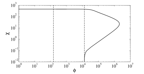
Figure 7: A plot of the boundary in field space on which quantum fluctuations become greater than the classical rolling of the fields. The three regions, described in the text, demarcate initial conditions on the surface for which $\chi$ does not reach $\chi=0$ before $\phi$ reaches $\phi_{\rm crit}$ (far left), initial conditions which do (middle), and initial conditions for which eternal inflation does not end (far right). Because of the symmetry of the potential, only positive values of $\phi$ and $\chi$ are shown.

IX Conclusions

In this paper we have demonstrated that inflation sourced by the hybrid potential Eq. (1) can give rise to an observationally significant non-Gaussianity while satisfying WMAP constraints on the power spectrum. The conditions required for this are summarised in Eq. (15). This is an example of the hilltop mechanism for producing non-Gaussianity first identified for axion models in Ref. Kim:2010ud .

In contrast with original hybrid inflation, where the waterfall field is heavy and cannot contribute significantly to the curvature perturbation on large scales heavy , we take the waterfall field to be light. Our scenario also leads to more than $60$ e-folds of accelerated expansion after the waterfall transition. This avoids issues of primordial black holes and domain walls. While earlier work has considered the hybrid model with a light waterfall field and the resulting non-Gaussianity barnaby ; Abolhasani:2011yp (and hybrid inflation with two light inflaton fields largeNG1 ; inhom2 ), we believe that our work is the only study of non-Gaussianity in the case in which more than $60$ e-folds of evolution occurs after the hybrid transition.

Numerically we have only exhaustively studied the range of parameters discussed in Section VII, but we have also probed several other parameter choices which lead to $60$ e-folds after the hybrid transition, including a number which are outside of the regime summarised by Eq. (15). Inside this regime analytic expectations are confirmed remarkably well by our simulations, which suggests that we should be able to trust them even outside it as long as the assumptions thay are based on are satisfied. Outside of this regime our non-exhaustive probing has not found any parameter choices which lead to a significant non-Gaussianity. It would be interesting, however, to probe an extended parameter range more carefully in order to determine whether the conditions Eq. (15) are the only ones which lead to a signal.

Finally we note that as discussed in Section VI an interesting feature of the hybrid model is that it offers an explanation for the initial conditions at horizon crossing which lead to a large non-Gaussianity. While parameter choices are necessarily fine tuned, therefore, the initial conditions need not be, at least for some subset of the parameters which can produce a large non-Gaussianity. This is in contrast to other two field models which produce a large non-Gaussianity due to inflationary dynamics largeNG1 ; largeNG2 ; Elliston:2011dr , which require both carefully choosen model parameters, and offer no explanation for the origin of the finely tuned horizon crossing conditions.

References

- (1) A. A. Starobinsky, Phys. Lett. 91B, 99 (1980); A. H. Guth, Phys. Rev. D 23, 347 (1981); A. Albrecht and P. J. Steinhardt, Phys. Rev. Lett. 48, 1220 (1982); S. W. Hawking and I. G. Moss, Phys. Lett. 110B, 35 (1982); A. D. Linde, Phys. Lett. 108B, 389 (1982); A. D. Linde, Phys. Lett. 129B, 177 (1983).
- (2) J. E. Lidsey, A. R. Liddle, E. W. Kolb, E. J. Copeland, T. Barreiro, and M. Abney, Rev. Mod. Phys. 69, 373 (1997), astro-ph/9508078; D. H. Lyth and A. Riotto, Phys. Rep. 314, 1 (1999), hep-ph/9807278; A. R. Liddle and D. H. Lyth, Cosmological Inflation and Large-Scale Structure (Cambridge University Press, Cambridge, 2000); B. A. Bassett, S. Tsujikawa, and D. Wands, astro-ph/0507632.
- (3) D. N. Spergel et al. [WMAP Collaboration], Astrophys. J. Suppl. 170, 377 (2007) [arXiv:astro-ph/0603449]; D. N. Spergel et al. [WMAP Collaboration], Astrophys. J. Suppl. 148, 175 (2003) [arXiv:astro-ph/0302209]; H. V. Peiris et al., Astrophys. J. Suppl. 148, 213 (2003), astro-ph/0302225.
- (4) E. Komatsu et al., arXiv:1001.4538 [astro-ph.CO];
- (5) J. M. Maldacena, JHEP 0305, 013 (2003). [astro-ph/0210603].
- (6) J. M. Bardeen, P. J. Steinhardt, M. S. Turner, Phys. Rev. D28, 679 (1983),
- (7) D. H. Lyth, Phys. Rev. D31, 1792-1798 (1985).
- (8) D. H. Lyth, K. A. Malik, M. Sasaki, JCAP 0505, 004 (2005). [astro-ph/0411220], G. I. Rigopoulos, E. P. S. Shellard, Phys. Rev. D68, 123518 (2003). [astro-ph/0306620], D. Langlois and F. Vernizzi, Phys. Rev. D 72, 103501 (2005) [arXiv:astro-ph/0509078].
- (9) D. H. Lyth and Y. Rodriguez, Phys. Rev. Lett. 95, 121302 (2005) [arXiv:astro-ph/0504045].
- (10) F. Vernizzi, D. Wands, JCAP 0605, 019 (2006). [astro-ph/0603799].
- (11) G. I. Rigopoulos, E. P. S. Shellard, B. J. W. van Tent, Phys. Rev. D73, 083521 (2006). [astro-ph/0504508]; G. I. Rigopoulos, E. P. S. Shellard, B. J. W. van Tent, Phys. Rev. D76, 083512 (2007). [astro-ph/0511041]; S. Yokoyama, T. Suyama and T. Tanaka, JCAP 0707, 013 (2007) [arXiv:0705.3178 [astro-ph]]; S. Yokoyama, T. Suyama and T. Tanaka, JCAP 0707, 013 (2007) [arXiv:0705.3178 [astro-ph]]; S. Yokoyama, T. Suyama and T. Tanaka, Phys. Rev. D 77, 083511 (2008) [arXiv:0711.2920 [astro-ph]]; D. J. Mulryne, D. Seery, D. Wesley, JCAP 1104, 030 (2011). [arXiv:1008.3159 [astro-ph.CO]]; D. J. Mulryne, D. Seery, D. Wesley, JCAP 1001, 024 (2010). [arXiv:0909.2256 [astro-ph.CO]].
- (12) L. Alabidi, JCAP 0610, 015 (2006). [astro-ph/0604611]; JCAP 0902, 017 (2009). [arXiv:0812.0807 [astro-ph]].
- (13) C. T. Byrnes, K. -Y. Choi, L. M. H. Hall, JCAP 0810 (2008) 008. [arXiv:0807.1101 [astro-ph]]; C. T. Byrnes, K. -Y. Choi, L. M. H. Hall, C. M. Peterson, M. Tegmark, [arXiv:1011.6675 [astro-ph.CO]].
- (14) J. Elliston, D. J. Mulryne, D. Seery, R. Tavakol, [arXiv:1106.2153 [astro-ph.CO]]; J. Elliston, D. Mulryne, D. Seery, R. Tavakol, [arXiv:1107.2270 [astro-ph.CO]].
- (15) S. A. Kim, A. R. Liddle, D. Seery, Phys. Rev. Lett. 105, 181302 (2010). [arXiv:1005.4410 [astro-ph.CO]].
- (16) S. Mollerach, Phys. Rev. D 42 (1990) 313; A. D. Linde and V. F. Mukhanov, Phys. Rev. D 56, 535 (1997) [arXiv:astro-ph/9610219]; D. H. Lyth and D. Wands, Phys. Lett. B 524, 5 (2002) [arXiv:hep-ph/0110002]; T. Moroi and T. Takahashi, Phys. Lett. B 522, 215 (2001) [Erratum-ibid. B 539, 303 (2002)] [arXiv:hep-ph/0110096]; K. Enqvist and S. Nurmi, JCAP 0510, 013 (2005) [arXiv:astro-ph/0508573]; A. Linde and V. Mukhanov, JCAP 0604, 009 (2006) [arXiv:astro-ph/0511736]; K. A. Malik and D. H. Lyth, JCAP 0609, 008 (2006) [arXiv:astro-ph/0604387]; M. Sasaki, J. Valiviita and D. Wands, Phys. Rev. D 74, 103003 (2006) [arXiv:astro-ph/0607627]; A. Chambers, S. Nurmi, A. Rajantie, JCAP 1001, 012 (2010). [arXiv:0909.4535 [astro-ph.CO]].
- (17) A. Chambers, A. Rajantie, Phys. Rev. Lett. 100, 041302 (2008). [arXiv:0710.4133 [astro-ph]]; A. Chambers, A. Rajantie, JCAP 0808 (2008) 002. [arXiv:0805.4795 [astro-ph]]; J. R. Bond, A. V. Frolov, Z. Huang, L. Kofman, Phys. Rev. Lett. 103 (2009) 071301. [arXiv:0903.3407 [astro-ph.CO]].
- (18) L. Kofman, arXiv:astro-ph/0303614; G. Dvali, A. Gruzinov and M. Zaldarriaga, Phys. Rev. D 69, 023505 (2004) [arXiv:astro-ph/0303591]; M. Zaldarriaga, Phys. Rev. D69, 043508 (2004). [astro-ph/0306006]; F. Vernizzi, Phys. Rev. D69, 083526 (2004). [astro-ph/0311167]; K. Ichikawa, T. Suyama, T. Takahashi and M. Yamaguchi, Phys. Rev. D 78, 063545 (2008) [arXiv:0807.3988 [astro-ph]]; C. T. Byrnes, arXiv:0810.3913 [astro-ph]; T. Suyama and M. Yamaguchi, Phys. Rev. D 77, 023505 (2008) [arXiv:0709.2545 [astro-ph]].
- (19) F. Bernardeau and J. P. Uzan, Phys. Rev. D 66 (2002) 103506 [arXiv:hep-ph/0207295]; F. Bernardeau and J. P. Uzan, Phys. Rev. D 67, 121301 (2003) [arXiv:astro-ph/0209330]; F. Bernardeau and T. Brunier, Phys. Rev. D 76 (2007) 043526 [arXiv:0705.2501 [hep-ph]]; D. H. Lyth, JCAP 0511, 006 (2005) [arXiv:astro-ph/0510443]; M. P. Salem, Phys. Rev. D 72, 123516 (2005) [arXiv:astro-ph/0511146]; L. Alabidi and D. Lyth, JCAP 0608, 006 (2006) [arXiv:astro-ph/0604569].
- (20) M. Sasaki, Prog. Theor. Phys. 120, 159 (2008) [arXiv:0805.0974 [astro-ph]]; A. Naruko and M. Sasaki, Prog. Theor. Phys. 121, 193 (2009) [arXiv:0807.0180 [astro-ph]].
- (21) L. Alabidi, K. Malik, C. T. Byrnes, K. -Y. Choi, JCAP 1011, 037 (2010). [arXiv:1002.1700 [astro-ph.CO]].
- (22) A. D. Linde, Phys. Rev. D49, 748-754 (1994). [astro-ph/9307002].
- (23) E. J. Copeland, A. R. Liddle, D. H. Lyth, E. D. Stewart, D. Wands, Phys. Rev. D49, 6410-6433 (1994). [astro-ph/9401011]; G. R. Dvali, Q. Shafi, R. K. Schaefer, Phys. Rev. Lett. 73, 1886-1889 (1994). [hep-ph/9406319].
- (24) E. J. Copeland, S. Pascoli, A. Rajantie, Phys. Rev. D65, 103517 (2002). [hep-ph/0202031].
- (25) L. Randall, M. Soljacic, A. H. Guth, [hep-ph/9601296].
- (26) N. Barnaby, J. M. Cline, Phys. Rev. D73, 106012 (2006). [astro-ph/0601481]; N. Barnaby, J. M. Cline, Phys. Rev. D75, 086004 (2007). [astro-ph/0611750].
- (27) J. Garcia-Bellido, A. D. Linde, D. Wands, Phys. Rev. D54, 6040-6058 (1996). [astro-ph/9605094].
- (28) S. Clesse, Phys. Rev. D83, 063518 (2011). [arXiv:1006.4522 [gr-qc]].
- (29) A. A. Starobinsky, JETP Lett. 42, 152-155 (1985).
- (30) M. Sasaki, E. D. Stewart, Prog. Theor. Phys. 95, 71-78 (1996). [astro-ph/9507001].
- (31) D. Wands, K. A. Malik, D. H. Lyth, A. R. Liddle, Phys. Rev. D62, 043527 (2000). [astro-ph/0003278].
- (32) D. Seery, J. E. Lidsey, JCAP 0509, 011 (2005). [astro-ph/0506056]; D. Seery, J. E. Lidsey and M. S. Sloth, JCAP 0701, 027 (2007) [arXiv:astro-ph/0610210]; D. Seery, M. S. Sloth and F. Vernizzi, JCAP 0903, 018 (2009) [arXiv:0811.3934 [astro-ph]].
- (33) J. Garcia-Bellido, D. Wands, Phys. Rev. D53, 5437-5445 (1996). [astro-ph/9511029].
- (34) A. D. Linde, Phys. Scripta T15, 169 (1987); A. D. Linde, Phys. Lett. B175, 395-400 (1986).
- (35) D. H. Lyth, arXiv:1012.4617 [astro-ph.CO]; J. Fonseca, M. Sasaki and D. Wands, JCAP 1009, 012 (2010) [arXiv:1005.4053 [astro-ph.CO]]; A. A. Abolhasani and H. Firouzjahi, Phys. Rev. D 83, 063513 (2011) [arXiv:1005.2934 [hep-th]]; J. O. Gong and M. Sasaki, JCAP 1103, 028 (2011) [arXiv:1010.3405 [astro-ph.CO]]; D. Mulryne, D. Seery and D. Wesley, arXiv:0911.3550 [astro-ph.CO].
- (36) A. A. Abolhasani, H. Firouzjahi and M. Sasaki, arXiv:1106.6315 [astro-ph.CO].