Applications of Derandomization Theory in Coding

[chapter]constrcnsConstruction headings-newheadings headings-new headings0 headings0

Applications of Derandomization Theory in Coding by
Mahdi Cheraghchi Bashi Astaneh Master of Science (École Polytechnique Fédérale de Lausanne), 2005 A dissertation submitted in partial fulfillment of the
requirements for the degree of
Doctor of Philosophy in
Computer Science at the
School of Computer and Communication Sciences
École Polytechnique Fédérale de Lausanne Thesis Number: 4767 Committee in charge:
Emre Telatar, Professor (President)
Amin Shokrollahi, Professor (Thesis Director)
Rüdiger Urbanke, Professor
Venkatesan Guruswami, Associate Professor
Christopher Umans, Associate Professor

July 2010

.

Applications of Derandomization Theory in Coding

.

Abstract

Randomized techniques play a fundamental role in theoretical computer science and discrete mathematics, in particular for the design of efficient algorithms and construction of combinatorial objects. The basic goal in derandomization theory is to eliminate or reduce the need for randomness in such randomized constructions. Towards this goal, numerous fundamental notions have been developed to provide a unified framework for approaching various derandomization problems and to improve our general understanding of the power of randomness in computation. Two important classes of such tools are pseudorandom generators and randomness extractors. Pseudorandom generators transform a short, purely random, sequence into a much longer sequence that looks random, while extractors transform a weak source of randomness into a perfectly random one (or one with much better qualities, in which case the transformation is called a randomness condenser).

In this thesis, we explore some applications of the fundamental notions in derandomization theory to problems outside the core of theoretical computer science, and in particular, certain problems related to coding theory. First, we consider the wiretap channel problem which involves a communication system in which an intruder can eavesdrop a limited portion of the transmissions. We utilize randomness extractors to construct efficient and information-theoretically optimal communication protocols for this model.

Then we consider the combinatorial group testing problem. In this classical problem, one aims to determine a set of defective items within a large population by asking a number of queries, where each query reveals whether a defective item is present within a specified group of items. We use randomness condensers to explicitly construct optimal, or nearly optimal, group testing schemes for a setting where the query outcomes can be highly unreliable, as well as the threshold model where a query returns positive if the number of defectives pass a certain threshold.

Next, we use randomness condensers and extractors to design ensembles of error-correcting codes that achieve the information-theoretic capacity of a large class of communication channels, and then use the obtained ensembles for construction of explicit capacity achieving codes. Finally, we consider the problem of explicit construction of error-correcting codes on the Gilbert-Varshamov bound and extend the original idea of Nisan and Wigderson to obtain a small ensemble of codes, mostly achieving the bound, under suitable computational hardness assumptions.

Keywords: Derandomization theory, randomness extractors, pseudorandomness, wiretap channels, group testing, error-correcting codes.

Résumé

Les techniques de randomisation jouent un rôle fondamental en informatique théorique et en mathématiques discrètes, en particulier pour la conception d’algorithmes efficaces et pour la construction d’objets combinatoires. L’objectif principal de la théorie de dérandomisation est d’éliminer ou de réduire le besoin d’aléa pour de telles constructions. Dans ce but, de nombreuses notions fondamentales ont été développées, d’une part pour créer un cadre unifié pour aborder différents problèmes de dérandomisation, et d’autre part pour mieux comprendre l’apport de l’aléa en informatique. Les générateurs pseudo-aléatoires et les extracteurs sont deux classes importantes de tels outils. Les générateurs pseudo-aléatoires transforment une suite courte et purement aléatoire en une suite beaucoup plus longue qui parait aléatoire. Les extracteurs d’aléa transforment une source faiblement aléatoire en une source parfaitement aléatoire (ou en une source de meilleure qualité. Dans ce dernier cas, la transformation est appelée un condenseur d’aléa).

Dans cette thèse, nous explorons quelques applications des notions fondamentales de la théorie de dérandomisation à des problèmes périphériques à l’informatique théorique et en particulier à certains problèmes relevant de la théorie des codes. Nous nous intéressons d’abord au problème du canal à jarretière, qui consiste en un système de communication où un intrus peut intercepter une portion limitée des transmissions. Nous utilisons des extracteurs pour construire pour ce modèle des protocoles de communication efficaces et optimaux du point de vue de la théorie de l’information.

Nous étudions ensuite le problème du test en groupe combinatoire. Dans ce problème classique, on se propose de déterminer un ensemble d’objets défectueux parmi une large population, à travers un certain nombre de questions, où chaque réponse révèle si un objet défectueux appartient à un certain ensemble d’objets. Nous utilisons des condenseurs pour construire explicitement des tests de groupe optimaux ou quasi-optimaux, dans un contexte où les réponses aux questions peuvent être très peu fiables, et dans le modèle de seuil où le résultat d’une question est positif si le nombre d’objets défectueux dépasse un certain seuil.

Ensuite, nous utilisons des condenseurs et des extracteurs pour concevoir des ensembles de codes correcteurs d’erreurs qui atteignent la capacité (dans le sens de la théorie de l’information) d’un grand nombre de canaux de communications. Puis, nous utilisons les ensembles obtenus pour la construction de codes explicites qui atteignent la capacité. Nous nous intéressons finalement au problème de la construction explicite de codes correcteurs d’erreurs qui atteignent la borne de Gilbert–Varshamov et reprenons l’idée originale de Nisan et Wigderson pour obtenir un petit ensemble de codes dont la plupart atteignent la borne, sous certaines hypothèses de difficulté computationnelle.

Mots-clés: Théorie de dérandomisation, extracteurs d’aléa, pseudo-aléa, canaux à jarretière, test en groupe, codes correcteurs d’erreurs.

Acknowledgments

During my several years of study at EPFL, both as a Master’s student and a Ph.D. student, I have had the privilege of interacting with so many wonderful colleagues and friends who have been greatly influential in my graduate life. Despite being thousands of miles away from home, thanks to them my graduate studies turned out to be one of the best experiences of my life. These few paragraphs are an attempt to express my deepest gratitude to all those who made such an exciting experience possible.

My foremost gratitude goes to my adviser, Amin Shokrollahi, for not only making my academic experience at EPFL truly enjoyable, but also for numerous other reasons. Being not only a great adviser and an amazingly brilliant researcher but also a great friend, Amin is undoubtedly one of the most influential people in my life. Over the years, he has taught me more than I could ever imagine. Beyond his valuable technical advice on research problems, he has thought me how to be an effective, patient, and confident researcher. He would always insist on picking research problems that are worth thinking, thinking about problems for the joy of thinking and without worrying about the end results, and publishing only those results that are worth publishing. His mastery in a vast range of areas, from pure mathematics to engineering real-world solutions, has always greatly inspired for me to try learning about as many topics as I can and interacting with people with different perspectives and interests. I’m especially thankful to Amin for being constantly available for discussions that would always lead to new ideas, thoughts, and insights. Moreover, our habitual outside-work discussions in restaurants, on the way for trips, and during outdoor activities turned out to be a great source of inspiration for many of our research projects, and in fact some of the results presented in this thesis! I’m also grateful to Amin for his collaborations on several research papers that we coauthored, as well as the technical substance of this thesis. Finally I thank him for numerous small things, like encouraging me to buy a car which turned out to be a great idea!

Secondly, I would like to thank our secretary Natascha Fontana for being so patient with too many inconveniences that I made for her over the years! She was about the first person I met in Switzerland, and kindly helped me settle in Lausanne and get used to my new life there. For several years I have been constantly bugging her with problems ranging from administrative trouble with the doctoral school to finding the right place to buy curtains. She has also been a great source of encouragement and support for my graduate studies.

Besides Amin and Natascha, I’m grateful to the present and past members of our Laboratory of Algorithms (ALGO) and Laboratory of Algorithmic Mathematics (LMA) for creating a truly active and enjoyable atmosphere: Bertrand Meyer, Ghid Maatouk, Giovanni Cangiani, Harm Cronie, Hesam Salavati, Luoming Zhang, Masoud Alipour, Raj Kumar (present members), and Andrew Brown, Bertrand Ndzana Ndzana, Christina Fragouli, Frédéric Didier, Frédérique Oggier, Lorenz Minder, Mehdi Molkaraie, Payam Pakzad, Pooya Pakzad, Zeno Crivelli (past members), as well as Alex Vardy, Emina Soljanin, Martin Fürer, and Shahram Yousefi (long-term visitors). Special thanks to:

Alex Vardy and Emina Soljanin: For fruitful discussions on the results presented in Chapter 3.

Frédéric Didier: For numerous fruitful discussions and his collaboration on our joint paper [ref:CDS09], on which Chapter 3 is based.

Giovanni Cangiani: For being a brilliant system administrator (along with Damir Laurenzi), and his great help with some technical problems that I had over the years.

Ghid Maatouk: For her lively presence as an endless source of fun in the lab, for taking student projects with me prior to joining the lab, helping me keep up my obsession about classical music, encouraging me to practice the piano, and above all, being an amazing friend. I also thank her and Bertrand Meyer for translating the abstract of my thesis into French.

Lorenz Minder: For sharing many tech-savvy ideas and giving me a quick campus tour when I visited him for a day in Berkeley, among other things.

Payam Pakzad: For many fun activities and exciting discussions we had during the few years he was with us in ALGO.

Zeno Crivelli and Bertrand Ndzana Ndzana: For sharing their offices with me for several years! I also thank Zeno for countless geeky discussions, lots of fun we had in the office, and for bringing a small plant to the office, which quickly grew to reach the ceiling and stayed fresh for the entire duration of my Ph.D. work.

I’m thankful to professors and instructors from whom I learned a great deal attending their courses as a part of my Ph.D. work: I learned Network Information Theory from Emre Telatar, Quantum Information Theory from Nicolas Macris, Algebraic Number Theory from Eva Bayer, Network Coding from Christina Fragouli, Wireless Communication from Suhas Diggavi, and Modern Coding Theory from my adviser Amin. As a teaching assistant, I also learned a lot from Amin’s courses (on algorithms and coding theory) and from an exciting collaboration with Monika Henzinger for her course on advanced algorithms.

During summer 2009, I spent an internship at KTH working with Johan Håstad and his group. What I learned from Johan within this short time turned out far more than I had expected. He was always available for discussions and listening to my countless silly ideas with extreme patience, and I would always walk out of his office with new ideas (ideas that would, contrary to those of my own, always work!). Working with the theory group at KTH was more than enjoyable, and I’m particularly thankful to Ola Svensson, Marcus Isaksson, Per Austrin, Cenny Wenner, and Lukáš Poláček for numerous delightful discussions.

Special thanks to cool fellows from the Information Processing Group (IPG) of EPFL for the fun time we had and also countless games of Foosball we played (brought to us by Giovanni).

I’m indebted to my great friend, Soheil Mohajer, for his close friendship over the years. Soheil has always been patient enough to answer my countless questions on information theory and communication systems in a computer-science-friendly language, and his brilliant mind has never failed to impress me. We had tons of interesting discussions on virtually any topic, some of which coincidentally (and finally!) contributed to a joint paper [ref:CKMS10]. I also thank Amin Karbasi and Venkatesh Saligrama for this work. Additional thanks goes to Amin for our other joint paper [ref:CHKV09] (along with Ali Hormati and Martin Vetterli whom I also thank) and in particular giving me the initial motivation to work on these projects, plus his unique sense of humor and amazing friendship over the years.

I’d like to extend my warmest gratitude to Pedram Pedarsani, for too many reasons to list here, but above all for being an amazingly caring and supportive friend and making my graduate life even more pleasing. Same goes to Mahdi Jafari, who has been a great friend of mine since middle school! Mahdi’s many qualities, including his humility, great mind, and perspective to life (not to mention great photography skills) has been a big influence on me. I feel extremely lucky for having such amazing friends.

I take this opportunity to thank three of my best, most brilliant, and most influential friends; Omid Etesami, Mohammad Mahmoody, and Ehsan Ardestanizadeh, whom I’m privileged to know since high school. In college, Omid showed me some beauties of complexity theory which strongly influenced me in pursuing my post-graduate studies in theoretical computer science. He was also influential in my decision to study at EPFL, which turned out to be one of my best decisions in life. I had the most fascinating time with Mohammad and Ehsan during their summer internships at EPFL. Mohammad thought me a great deal about his fascinating work on foundations of cryptography and complexity theory and was always up to discuss anything ranging from research ideas to classical music and cinema. I worked with Ehsan on our joint paper [ref:ACS09] which turned out to be one of the most delightful research collaborations I’ve had. Ehsan’s unique personality, great wit and sense of humor, as well as musical talents—especially his mastery in playing Santur—has always filled me with awe. I also thank the three of them for keeping me company and showing me around during my visits in Berkeley, Princeton, and San Diego.

In addition to those mentioned above, I’m grateful to so many amazing friends who made my study in Switzerland an unforgettable stage of my life and full of memorable moments: Ali Ajdari Rad, Amin Jafarian, Arash Golnam, Arash Salarian, Atefeh Mashatan, Banafsheh Abasahl, Elham Ghadiri, Faezeh Malakouti, Fereshteh Bagherimiyab, Ghazale Hosseinabadi, Hamed Alavi, Hossein Afshari, Hossein Rouhani, Hossein Taghavi, Javad Ebrahimi, Laleh Golestanirad, Mani Bastani Parizi, Marjan Hamedani, Marjan Sedighi, Maryam Javanmardy, Maryam Zaheri, Mina Karzand, Mohammad Karzand, Mona Mahmoudi, Morteza Zadimoghaddam, Nasibeh Pouransari, Neda Salamati, Nooshin Hadadi, Parisa Haghani, Pooyan Abouzar, Pouya Dehghani, Ramtin Pedarsani, Sara Kherad Pajouh, Shirin Saeedi, Vahid Aref, Vahid Majidzadeh, Wojciech Galuba, and Zahra Sinaei. Each name should have been accompanied by a story (ranging from a few lines to a few pages); however, doing so would have made this section exceedingly long. Moreover, having prepared the list rather hastily, I’m sure I have missed a lot of nice friends on it. I owe them a coffee (or tea, if they prefer) each! Additional thanks to Mani, Ramtin, and Pedram, for their musical presence.

Thanks to Alon Orlitsky, Avi Wigderson, Madhu Sudan, Rob Calderbank, and Umesh Vazirani for arranging my short visits to UCSD, IAS, MIT, Princeton, and U.C. Berkeley, and to Anup Rao, Swastik Kopparty, and Zeev Dvir for interesting discussions during those visits.

I’m indebted to Chris Umans, Emre Telatar, Rüdiger Urbanke, and Venkat Guruswami for giving me the honor of having them in my dissertation committee. I also thank them (and Amin) for carefully reading the thesis and their comments on an earlier draft of this work. Additionally, thanks to Venkat for numerous illuminating discussions on various occasions, in particular on my papers [ref:Che09, ref:Che10] that form the basis of the material presented in Chapter 4.

My work was in part funded by grants from the Swiss National Science Foundation (Grant No. 200020-115983/1) and the European Research Council (Advanced Grant No. 228021) that I gratefully acknowledge.

Above all, I express my heartfelt gratitude to my parents, sister Azadeh, and brother Babak who filled my life with joy and happiness. Without their love, support, and patience none of my achievements—in particular this thesis—would have been possible. I especially thank my mother for her everlasting love, for all she went through until I reached this point, and her tremendous patience during my years of absence while I was only able to go home for a short visit each year. This thesis is dedicated with love to her.

*

Chapter 1 Introduction

70

Over the decades, the role of randomness in computation has proved to be one of the most intriguing subjects of study in computer science. Considered as a fundamental computational resource, randomness has been extensively used as an indispensable tool in design and analysis of algorithms, combinatorial constructions, cryptography, and computational complexity.

As an illustrative example on the power of randomness in algorithms, consider a clustering problem, in which we wish to partition a collection of items into two groups. Suppose that some pairs of items are marked as inconsistent, meaning that they are best be avoided falling in the same group. Of course, it might be simply impossible to group the items in such a way that no inconsistencies occur within the two groups. For that reason, it makes sense to consider the objective of minimizing the number of inconsistencies induced by the chosen partitioning. Suppose that we are asked to color individual items red or blue, where the items marked by the same color form each of the two groups. How can we design a strategy that maximizes the number of inconsistent pairs that fall in different groups? The basic rule of thumb in randomized algorithm design suggests that

When unsure making decisions, try flipping coins!

Thus a naive strategy for assigning color to items would be to flip a fair coin for each item. If the coin falls Heads, we mark the item blue, and otherwise red.

How can the above strategy possibly be any reasonable? After all we are defining the groups without giving the slightest thought on the given structure of the inconsistent pairs! Remarkably, a simple analysis can prove that the coin-flipping strategy is in fact a quite reasonable one. To see why, consider any inconsistent pair. The chance that the two items are assigned the same color is exactly one half. Thus, we expect that half of the inconsistent pairs end up falling in different groups. By repeating the algorithm a few times and checking the outcomes, we can be sure that an assignment satisfying half of the inconsistency constraints is found after a few trials.

We see that, a remarkably simple algorithm that does not even read its input can attain an approximate solution to the clustering problem in which the number of inconsistent pairs assigned to different groups is no less than half the maximum possible. However, our algorithm used a valuable resource; namely random coin flips, that greatly simplified its task. In this case, it is not hard to come up with an efficient (i.e., polynomial-time) algorithm that does equally well without using any randomness. However, designing such an algorithm and analyzing its performance is admittedly a substantially more difficult task that what we demonstrated within a few paragraphs above.

As it turns out, finding an optimal solution to our clustering problem above is an intractable problem (in technical terms, it is $\mathsf{NP}$-hard), and even obtaining an approximation ratio better than $16/17\approx.941$ is so [HastadOptimal]. Thus the trivial bit-flipping algorithm indeed obtains a reasonable solution. In a celebrated work, Goemans and Williamson [ref:GW95] improve the approximation ratio to about $.878$, again using randomization. A deterministic algorithm achieving the same quality was later discovered [ref:MR95], though it is much more complicated to analyze.

Another interesting example demonstrating the power of randomness in algorithms is the primality testing problem, in which the goal is to decide whether a given $n$-digit integer is prime or composite. While efficient (polynomial-time in $n$) randomized algorithms were discovered for this problem as early as 1970’s (e.g., Solovay-Strassen’s [ref:SS77] and Miller-Rabin’s algorithms [ref:Mil76, ref:Rab80]), a deterministic polynomial-time algorithm for primality testing was found decades later, with the breakthrough work of Agrawal, Kayal, and Saxena [ref:AKS04], first published in 2002. Even though this algorithm provably works in polynomial time, randomized methods still tend to be more favorable and more efficient for practical applications.

The primality testing algorithm of Agrawal et al. can be regarded as a derandomization of a particular instance of the polynomial identity testing problem. Polynomial identity testing generalizes the high-school-favorite problem of verifying whether a pair of polynomials expressed as closed form formulae expand to identical polynomials. For example, the following is an 8-variate identity

$$(x_{1}^{2}+x_{2}^{2}+x_{3}^{2}+x_{4}^{2})(y_{1}^{2}+y_{2}^{2}+y_{3}^{2}+y_{4}^{2})\stackrel{{\scriptstyle?}}{{\equiv}}\\ (x_{1}y_{1}-x_{2}y_{2}-x_{3}y_{3}-x_{4}y_{4})^{2}+(x_{1}y_{2}+x_{2}y_{1}+x_{3}y_{4}-x_{4}y_{3})^{2}+\\ (x_{1}y_{3}-x_{2}y_{4}+x_{3}y_{1}+x_{4}y_{2})^{2}+(x_{1}y_{4}+x_{2}y_{3}-x_{3}y_{2}+x_{4}y_{1})^{2}$$

which turns out to be valid. When the number of variables and the complexity of the expressions grow, the task of verifying identities becomes much more challenging using naive methods.

This is where the power of randomness comes into play again. A fundamental idea due to Schwartz and Zippel [ref:Schwartz, ref:Zippel] shows that the following approach indeed works:

Evaluate the two polynomials at sufficiently many randomly chosen points, and identify them as identical if and only if all evaluations agree.

It turns out that the above simple idea leads to a randomized efficient algorithm for testing identities that may err with an arbitrarily small probability. Despite substantial progress, to this date no polynomial-time deterministic algorithms for solving general identity testing problem is known, and a full derandomization of Schwartz-Zippel’s algorithm remains a challenging open problem in theoretical computer science.

The discussion above, among many other examples, makes the strange power of randomness evident. Namely, in certain circumstances the power of randomness makes algorithms more efficient, or simpler to design and analyze. Moreover, it is not yet clear how to perform certain computational tasks (e.g., testing for general polynomial identities) without using randomness.

Apart from algorithms, randomness has been used as a fundamental tool in various other areas, a notable example being combinatorial constructions. Combinatorial objects are of fundamental significance for a vast range of theoretical and practical problems. Often solving a practical problem (e.g., a real-world optimization problem) reduces to construction of suitable combinatorial objects that capture the inherent structure of the problem. Examples of such combinatorial objects include graphs, set systems, codes, designs, matrices, or even sets of integers. For these constructions, one has a certain structural property of the combinatorial object in mind (e.g., mutual intersections of a set system consisting of subsets of a universe) and seeks for an instance of the object that optimizes the property in mind in the best possible way (e.g., the largest possible set system with bounded mutual intersections).

The task of constructing suitable combinatorial objects turns out quite challenging at times. Remarkably, in numerous situations the power of randomness greatly simplifies the task of constructing the ideal object. A powerful technique in combinatorics, dubbed as the probabilistic method (see [probMethod]) is based on the following idea:

When out of ideas finding the right combinatorial object, try a random one!

Surprisingly, in many cases this seemingly naive strategy significantly beats the most brilliant constructions that do not use any randomness. An illuminating example is the problem of constructing Ramsey graphs. It is well known that in a group of six or more people, either there are at least three people who know each other or three who do not know each other. More generally, Ramsey theory shows that for every positive integer $K$, there is an integer $N$ such that in a group of $N$ or more people, either there are at least $K$ people who mutually know each other (called a clique of size $K$) or $K$ who are mutually unfamiliar with one another (called an independent set of size $K$). Ramsey graphs capture the reverse direction:

For a given $N$, what is the smallest $K$ such that there is a group of $N$ people with no cliques or independent sets of size $K$ or more? And how can an example of such a group be constructed?

In graph-theoretic terms (where mutual acquaintances are captured by edges), an undirected graph with $N:=2^{n}$ vertices is called a Ramsey graph with entropy $k$ if it has no clique or independent set of size $K:=2^{k}$ (or larger). The Ramsey graph construction problem is to efficiently construct a graph with smallest possible entropy $k$.

Constructing a Ramsey graph with entropy $k=(n+1)/2$ is already nontrivial. However, the following Hadamard graph does the job [CG88]: Each vertex of the graph is associated with a binary vector of length $n$, and there is an edge between two vertices if their corresponding vectors are orthogonal over the binary field. A much more involved construction, due to Barak et al. [BRSW06] (which remains the best deterministic construction to date) attain an entropy $k=n^{o(1)}$.

A brilliant, but quite simple, idea due to Erdős [Erdos] demonstrates the power of randomness in combinatorial constructions: Construct the graph randomly, by deciding whether to put an edge between every pair of vertices by flipping a fair coin. It is easy to see that the resulting graph is, with overwhelming probability, a Ramsey graph with entropy $k=\log n+2$. It also turns out that this is about the lowest entropy one can hope for! Note the significant gap between what achieved by a simple, probabilistic construction versus what achieved by the best known deterministic constructions.

Even though the examples discussed above clearly demonstrate the power of randomness in algorithm design and combinatorics, a few issues are inherently tied with the use of randomness as a computational resource, that may seem unfavorable:

1. A randomized algorithm takes an abundance of fair, and independent, coin flips for granted, and the analysis may fall apart if this assumption is violated. For example, in the clustering example above, if the coin flips are biased or correlated, the $.5$ approximation ratio can no longer be guaranteed. This raises a fundamental question:

   Does “pure randomness” even exist? If so, how can we instruct a computer program to produce purely random coin flips?

2. Even though the error probability of randomized algorithms (such as the primality testing algorithms mentioned above) can be made arbitrarily small, it remains nonzero. In certain cases where a randomized algorithm never errs, its running time may vary depending on the random choices being made. We can never be completely sure whether an error-prone algorithm has really produced the right outcome, or whether one with a varying running time is going to terminate in a reasonable amount of time (even though we can be almost confident that it does).

3. As we saw for Ramsey graphs, the probabilistic method is a powerful tool in showing that combinatorial objects with certain properties exist, and it most cases it additionally shows that a random object almost surely achieves the desired properties. Even though for certain applications a randomly produced object is good enough, in general there might be no easy way to certify whether a it indeed satisfies the properties sought for. For the example of Ramsey graphs, while almost every graph is a Ramsey graph with a logarithmically small entropy, it is not clear how to certify whether a given graph satisfies this property. This might be an issue for certain applications, when an object with guaranteed properties is needed.

The basic goal of derandomization theory is to address the above-mentioned and similar issues in a systematic way. A central question in derandomization theory deals with efficient ways of simulating randomness, or relying on weak randomness when perfect randomness (i.e., a steady stream of fair and independent coin flips) is not available. A mathematical formulation of randomness is captured by the notion of entropy, introduced by Shannon [ref:Shannon], that quantifies randomness as the amount of uncertainty in the outcome of a process. Various sources of “unpredictable” phenomena can be found in nature. This can be in form of an electric noise, thermal noise, ambient sound input, image captured by a video camera, or even a user’s input given to an input device such as a keyboard. Even though it is conceivable to assume that a bit-sequence generated by all such sources contains a certain amount of entropy, the randomness being offered might be far from perfect. Randomness extractors are fundamental combinatorial, as well as computational, objects that aim to address this issue.

As an example to illustrate the concept of extractors, suppose that we have obtained several independent bit-streams $X_{1},X_{2},\ldots,X_{r}$ from various physically random sources. Being obtained from physical sources, not much is known about the structure of these sources, and the only assumption that we can be confident about is that they produce a substantial amount of entropy. An extractor is a function that combines these sources into one, perfectly random, source. In symbols, we have

$$f(X_{1},X_{2},\ldots,X_{r})=Y,$$

where the output source $Y$ is purely random provided that the input sources are reasonably (but not fully) random. To be of any practical use, the extractor $f$ must be efficiently computable as well. A more general class of functions, dubbed condensers are those that do not necessarily transform imperfect randomness into perfect one, but nevertheless substantially purifies the randomness being given. For instance, as a condenser, the function $f$ may be expected to produce an output sequence whose entropy is $90\%$ of the optimal entropy offered by perfect randomness.

Intuitively, there is a trade-off between structure and randomness. A sequence of fair coin flips is extremely unpredictable in that one cannot bet on predicting the next coin flip and expect to gain any advantage out of it. On the other extreme, a sequence such as what given by digits of $\pi=3.14159265\dots$ may look random but is in fact perfectly structured. Indeed one can use a computer program to perfectly predict the outcomes of this sequence. A physical source, on the other hand, may have some inherent structure in it. In particular, the outcome of a physical process at a certain point might be more or less predictable, dictated by physical laws, from the outcomes observed immediately prior to that time. However, the degree of predictability may of course not be as high as in the case of $\pi$.

From a combinatorial point of view, an extractor is a combinatorial object that neutralizes any kind of structure that is inherent in a random source, and, extracts the “random component” out (if there is any). On the other hand, in order to be any useful, an extractor must be computationally efficient. At a first sight, it may look somewhat surprising to learn that such objects may even exist! In fact, as in the case of Ramsey graphs, the probabilistic method can be used to show that a randomly chosen function is almost surely a decent extractor. However, a random function is obviously not good enough as an extractor since the whole purpose of an extractor is to eliminate the need for pure randomness. Thus for most applications, an extractor (and more generally, condenser) is required to be efficiently computable and utilize as small amount of auxiliary pure randomness as possible.

While randomness extractors were originally studied for the main purpose of eliminating the need for pure randomness in randomized algorithms, they have found surprisingly diverse applications in different areas of combinatorics, computer science, and related fields. Among many such developments, one can mention construction of good expander graphs [WZ99] and Ramsey graphs [BRSW06] (in fact the best known construction of Ramsey graphs can be considered a byproduct of several developments in extractor theory), communication complexity [CG88], Algebraic complexity theory [ref:RY08], distributed computing (e.g., [Zuc97, GVZ06, RZ01]), data structures (e.g., [ref:Ta02]), hardness of optimization problems [MU01, Zuc96], cryptography (see, e.g., [ref:Dodis]), coding theory [ref:TZ04], signal processing [ref:Ind08], and various results in structural complexity theory (e.g., [GZ97]).

In this thesis we extend such connections to several fundamental problems related to coding theory. In the following we present a brief summary of the individual problems that are studied in each chapter.

The Wiretap Channel Problem

The wiretap channel problem studies reliable transmission of messages over a communication channel which is partially observable by a wiretapper. As a basic example, suppose that we wish to transmit a sensitive document over the internet. Loosely speaking, the data is transmitted in form of packets, consisting of blocks of information, through the network.

Packets may be transmitted along different paths over the network through a cloud of intermediate transmitters, called routers, until delivered at the destination. Now an adversary who has access to a set of the intermediate routers may be able to learn a substantial amount of information about the message being transmitted, and thereby render the communication system insecure.

A natural solution for assuring secrecy in transmission is to use a standard cryptographic scheme to encrypt the information at the source. However, the information-theoretic limitation of the adversary in the above scenario (that is, the fact that not all of the intermediate routers, but only a limited number of them are being eavesdropped) makes it possible to provably guarantee secure transmission by using a suitable encoding at the source. In particular, in a wiretap scheme, the original data is encoded at the source to a slightly redundant sequence, that is then transmitted to the recipient. As it turns out, the scheme can be designed in such a way that no information is leaked to the intruder and moreover no secrets (e.g., an encryption key) need to be shared between the two parties prior to transmission.

We study this problem in Chapter 3. The main contribution of this chapter is a construction of information-theoretically secure and optimal wiretap schemes that guarantee secrecy in various settings of the problem. In particular the scheme can be applied to point-to-point communication models as well as networks, even in presence of noise or active intrusion (i.e., when the adversary not only eavesdrops, but also alters the information being transmitted). The construction uses an explicit family of randomness extractors as the main building block.

Combinatorial Group Testing

Group testing is a classical combinatorial problem that has applications in surprisingly diverse and seemingly unrelated areas, from data structures to coding theory to biology.

Intuitively, the problem can be described as follows: Suppose that blood tests are taken from a large population (say hundreds of thousands of people), and it is suspected that a small number (e.g., up to one thousand) carry a disease that can be diagnosed using costly blood tests. The idea is that, instead of testing blood samples one by one, it might be possible to pool them in fairly large groups, and then apply the tests on the groups without affecting reliability of the tests. Once a group is tested negative, all the samples participating in the group must be negative and this may save a large number of tests. Otherwise, a positive test reveals that at least one of the individuals in the group must be positive (though we do not learn which).

The main challenge in group testing is to design the pools in such a way to allow identification of the exact set of infected population using as few tests as possible, thereby economizing the identification process of the affected individuals. In Chapter 4 we study the group testing problem and its variations. In particular, we consider a scenario where the tests can produce highly unreliable outcomes, in which case the scheme must be designed in such a way that allows correction of errors caused by the presence of unreliable measurements. Moreover, we study a more general threshold variation of the problem in which a test returns positive if the number of positives participating in the test surpasses a certain threshold. This is a more reasonable model than the classical one, when the tests are not sufficiently sensitive and may be affected by dilution of the samples pooled together. In both models, we will use randomness condensers as combinatorial building blocks for construction of optimal, or nearly optimal, explicit measurement schemes that also tolerate erroneous outcomes.

Capacity Achieving Codes

The theory of error-correcting codes aims to guarantee reliable transmission of information over an unreliable communication medium, known in technical terms as a channel. In a classical model, messages are encoded into sequences of bits at their source, which are subsequently transmitted through the channel. Each bit being transmitted through the channel may be flipped (from $0$ to $1$ or vice versa) with a small probability.

Using an error-correcting code, the encoded sequence can be designed in such a way to allow correct recovery of the message at the destination with an overwhelming probability (over the randomness of the channel). However, the cost incurred by such an encoding scheme is a loss in the transmission rate, that is, the ratio between the information content of the original message and the length of the encoded sequence (or in other words, the effective number of bits transmitted per channel use).

A capacity achieving code is an error correcting code that essentially maximizes the transmission rate, while keeping the error probability negligible. The maximum possible rate depends on the channel being considered, and is a quantity given by the Shannon capacity of the channel.

In Chapter LABEL:chap:capacity, we consider a general class of communication channels (including the above example) and show how randomness condensers and extractors can be used to design capacity achieving ensembles of codes for them. We will then use the obtained ensembles to obtain explicit constructions of capacity achieving codes that allow efficient encoding and decoding as well.

Codes on the Gilbert-Varshamov Bound

While randomness extractors aim for eliminating the need for pure randomness in algorithms, a related class of objects known as pseudorandom generators aim for eliminating randomness altogether. This is made meaningful by a fundamental idea saying that randomness should be defined relative to the observer. The idea can be perhaps best described by an example due to Goldreich [ref:Gol08]*Chapter 8, quoted below:

“Alice and Bob play head or tail in one of the following four ways. In all of them Alice flips a coin high in the air, and Bob is asked to guess its outcome before the coin hits the floor. The alternative ways differ by the knowledge Bob has before making his guess.

In the first alternative, Bob has to announce his guess before Alice flips the coin. Clearly, in this case Bob wins with probability $1/2$.

In the second alternative, Bob has to announce his guess while the coin is spinning in the air. Although the outcome is determined in principle by the motion of the coin, Bob does not have accurate information on the motion. Thus we believe that, also in this case Bob wins with probability $1/2$.

The third alternative is similar to the second, except that Bob has at his disposal sophisticated equipment capable of providing accurate information on the coin’s motion as well as on the environment affecting the outcome. However, Bob cannot process this information in time to improve his guess.

In the fourth alternative, Bob’s recording equipment is directly connected to a powerful computer programmed to solve the motion equations and output a prediction. It is conceivable that in such a case Bob can improve substantially his guess of the outcome of the coin.”

Following the above description, in principle the outcome of a coin flip may well be deterministic. However, as long as the observer does not have enough resources to gain any advantage predicting the outcome, the coin flip should be considered random for him. In this example, what makes the coin flip random for the observer is the inherent hardness (and not necessarily impossibility) of the prediction procedure. The theory of pseudorandom generators aim to express this line of thought in rigorous ways, and study the circumstances under which randomness can be simulated for a particular class of observers.

The advent of probabilistic algorithms that are unparalleled by deterministic methods, such as randomized primality testing (before the AKS algorithm [ref:AKS04]), polynomial identity testing and the like initially made researchers believe that the class of problems solvable by randomized polynomial-time algorithms (in symbols, $\mathsf{BPP}$) might be strictly larger than those solvable in polynomial-time without the need for randomness (namely, $\mathsf{P}$) and conjecture $\mathsf{P}\neq\mathsf{BPP}$. To this date, the “$\mathsf{P}$ vs. $\mathsf{BPP}$” problem remains one of the most challenging problems in theoretical computer science.

Despite the initial belief, more recent research has led most theoreticians to believe otherwise, namely that $\mathsf{P}=\mathsf{BPP}$. This is supported by recent discovery of deterministic algorithms such as the AKS primality test, and more importantly, the advent of strong pseudorandom generators. In a seminal work [NW], Nisan and Wigderson showed that a “hard to compute” function can be used to efficiently transform a short sequence of random bits into a much longer sequence that looks indistinguishable from a purely random sequence to any efficient algorithm. In short, they showed how to construct pseudorandomness from hardness. Though the underlying assumption (that certain hard functions exists) is not yet proved, it is intuitively reasonable to believe (just in the same way that, in the coin flipping game above, the hardness of gathering sufficient information for timely prediction of the outcome by Bob is reasonable to believe without proof).

In Chapter LABEL:chap:gv we extend Nisan and Wigderson’s method (originally aimed for probabilistic algorithms) to combinatorial constructions and show that, under reasonable hardness assumptions, a wide range of probabilistic combinatorial constructions can be substantially derandomized.

The specific combinatorial problem that the chapter is based on is the construction of error-correcting codes that attain the rate versus error-tolerance trade-off shown possible using the probabilistic method (namely, construction of codes on the so-called Gilbert-Varshamov bound). In particular, we demonstrate a small ensemble of efficiently constructible error-correcting codes almost all of which being as good as random codes (under a reasonable assumption). Even though the method is discussed for construction of error-correcting codes, it can be equally applied to numerous other probabilistic constructions; e.g., construction of optimal Ramsey graphs.

Reading Guidelines

The material presented in each of the technical chapters of this thesis (Chapters 3–6) are presented independently so they can be read in any order. Since the theory of randomness extractors plays a central role in the technical content of this thesis, Chapter 2 is devoted to an introduction to this theory, and covers some basic constructions of extractors and condenser that are used as building blocks in the main chapters. Since the extractor theory is already an extensively developed area, we will only touch upon basic topics that are necessary for understanding the thesis.

Apart from extractors, we will extensively use fundamental notions of coding theory throughout the thesis. For that matter, we have provided a brief review of such notions in Appendix LABEL:app:coding.

The additional mathematical background required for each chapter is provided when needed, to the extent of not losing focus. For a comprehensive study of the basic tools being used, we refer the reader to [ref:MR, ref:MU, probMethod] (probability, randomness in algorithms, and probabilistic constructions), [HLW06] (expander graphs), [ref:AB09, ref:Gol08] (modern complexity theory), [ref:MS, ref:vanl, ref:Roth] (coding theory and basic algebra needed), [ref:Venkat] (list decoding), and [ref:groupTesting, ref:DH06] (combinatorial group testing).

Each chapter of the thesis is concluded by the opening notes of a piece of music that I truly admire.

   

Johann Sebastian Bach (1685–1750): The Art of Fugue BWV 1080, Contrapunctus XIV.

Chapter 2 Extractor Theory

70

Suppose that you are given a possibly biased coin that falls heads some $p$ fraction of times ($0<p<1$) and are asked to use it to “simulate” fair coin flips. A natural approach to solve this problem would be to first try to “learn” the bias $p$ by flipping the coin a large number of times and observing the fraction of times it falls heads during the experiment, and then using this knowledge to encode the sequence of biased flips to its information-theoretic entropy.

Remarkably, back in 1951 John von Neumann [vN51] demonstrated a simple way to solve this problem without knowing the bias $p$: flip the coin twice and one of the following cases may occur:

1. The first flip shows Heads and the second Tails: output “H”.

2. The first flip shows Tails and the second Heads: output “T”.

3. Otherwise, repeat the experiment.

Note that the probability that the output symbol is “H” is precisely equal to it being “T”, namely, $p(1-p)$. Thus, the outcome of this process represents a perfectly fair coin toss. This procedure might be somewhat wasteful; for instance, it is expected to waste half of the coin flips even if $p=1/2$ (that is, if the coin is already fair) and that is the cost we pay for not knowing $p$. But nevertheless, it transforms an imperfect, not fully known, source of randomness into a perfect source of random bits.

This example, while simple, demonstrates the basic idea in what is known as “extractor theory”. The basic goal in extractor theory is to improve randomness, that is, to efficiently transform a “weak” source of randomness into one with better qualities; in particular, having a higher entropy per symbol. The procedure shown above, seen as a function from the sequence of coin flips to a Boolean function (over $\{H,T\}$) is known as an extractor. It is called so since it “extracts” pure randomness from a weak source.

When the distribution of the weak source is known, it is possible to use techniques from source coding (say Huffman or Arithmetic Coding) to compress the information to a number of bits very close to its actual entropy, without losing any of the source information. What makes extractor theory particularly challenging is the following issues:

1. An extractor knows little about the exact source distribution. Typically nothing more than a lower bound on the source entropy, and no structure is assumed on the source. In the above example, even though the source distribution was unknown, it was known to be an i.i.d. sequence (i.e., a sequence of independent, identically distributed symbols). This need not be the case in general.

2. The output of the extractor must “strongly” resemble a uniform distribution (which is the distribution with maximum possible entropy), in the sense that no statistical test (no matter how complex) should be able to distinguish between the output distribution and a purely random sequence. Note, for example, that a sequence of $n-1$ uniform and independent bits followed by the symbol “$0$” has $n-1$ bits of entropy, which is only slightly lower than that of $n$ purely random bits (i.e., $n$). However, a simple statistical test can trivially distinguish between the two distributions by only looking at the last bit.

Since extractors and related objects (in particular, lossless condensers) play a central role in the technical core of this thesis, we devote this chapter to a formal treatment of extractor theory, introducing the basic ideas and some fundamental constructions. In this chapter, we will only cover basic notions and discuss a few of the results that will be used as building blocks in the rest of thesis.

1 Probability Distributions

1.1 Distributions and Distance

In this thesis we will focus on probability distributions over finite domains. Let $(\Omega,\mathsf{E},\mathcal{X})$ be a probability space, where $\Omega$ is a finite sample space, $\mathsf{E}$ is the set of events (that in our work, will always consist of the set of subsets of $\Omega$), and $\mathcal{X}$ is a probability measure. The probability assigned to each outcome $x\in\Omega$ by $\mathcal{X}$ will be denoted by $\mathcal{X}(x)$, or $\Pr_{\mathcal{X}}(x)$. Similarly, for an event $T\in\mathsf{E}$, we will denote the probability assigned to $T$ by $\mathcal{X}(T)$, or $\Pr_{\mathcal{X}}[T]$ (when clear from the context, we may omit the subscript $\mathcal{X}$). The support of $\mathcal{X}$ is defined as

$$\mathsf{supp}(\mathcal{X}):=\{x\in\Omega\colon\mathcal{X}(x)>0\}.$$

A particularly important probability measure is defined by the uniform distribution, which assigns equal probabilities to each element of $\Omega$. We will denote the uniform distribution over $\Omega$ by $\mathcal{U}_{\Omega}$, and use the shorthand $\mathcal{U}_{n}$, for an interger $n\geq 1$, for $\mathcal{U}_{\{0,1\}^{n}}$. We will use the notation $X\sim\mathcal{X}$ to denote that the random variable $X$ is drawn from the probability distribution $\mathcal{X}$.

It is often convenient to think about the probability measure as a real vector of dimension $|\Omega|$, whose entries are indexed by the elements of $\Omega$, such that the value at the $i$th entry of the vector is $\mathcal{X}(i)$.

An important notion for our work is the distance between distributions. There are several notions of distance in the literature, some stronger than the others, and often the most suitable choice depends on the particular application in hand. For our applications, the most important notion is the $\ell_{p}$ distance:

Definition 2.1.

Let $\mathcal{X}$ and $\mathcal{Y}$ be probability distributions on a finite domain $\Omega$. Then for every $p\geq 1$, their $\ell_{p}$ distance, denoted by $\|\mathcal{X}-\mathcal{Y}\|_{p}$, is given by

$$\|\mathcal{X}-\mathcal{Y}\|_{p}:=\left(\sum_{x\in\Omega}|\mathcal{X}(x)-\mathcal{Y}(y)|^{p}\right)^{1/p}.$$

We extend the distribution to the special case $p=\infty$, to denote the point-wise distance:

$$\|\mathcal{X}-\mathcal{Y}\|_{\infty}:=\max_{x\in\Omega}{|\mathcal{X}(x)-\mathcal{Y}(y)|}.$$

The distributions $\mathcal{X}$ and $\mathcal{Y}$ are called $\epsilon$-close with respect to the $\ell_{p}$ norm if and only if $\|\mathcal{X}-\mathcal{Y}\|_{p}\leq\epsilon$.

We remark that, by the Cauchy-Schwarz inequality, the following relationship between $\ell_{1}$ and $\ell_{2}$ distances holds:

$$\|\mathcal{X}-\mathcal{Y}\|_{2}\leq\|\mathcal{X}-\mathcal{Y}\|_{1}\leq\sqrt{|\Omega|}\cdot\|\mathcal{X}-\mathcal{Y}\|_{2}.$$

Of particular importance is the statistical (or total variation) distance. This is defined as half the $\ell_{1}$ distance between the distributions:

$$\|\mathcal{X}-\mathcal{Y}\|:=\textstyle\frac{1}{2}\|\mathcal{X}-\mathcal{Y}\|_{1}.$$

We may also use the notation ${\mathsf{dist}}(\mathcal{X},\mathcal{Y})$ to denote the statistical distance. We call two distributions $\epsilon$-close if and only if their statistical distance is at most $\epsilon$. When there is no risk of confusion, we may extend such notions as distance to the random variables they are sampled from, and, for instance, talk about two random variables being $\epsilon$-close.

This is in a sense, a very strong notion of distance since, as the following proposition suggests, it captures the worst-case difference between the probability assigned by the two distributions to any event:

Proposition 2.2.

Let $\mathcal{X}$ and $\mathcal{Y}$ be distributions on a finite domain $\Omega$. Then $\mathcal{X}$ and $\mathcal{Y}$ are $\epsilon$-close if and only if for every event $T\subseteq\Omega$, $|\Pr_{\mathcal{X}}[T]-\Pr_{\mathcal{Y}}[T]|\leq\epsilon$.

Proof.

Denote by $\Omega_{\mathcal{X}}$ and $\Omega_{\mathcal{Y}}$ the following partition of $\Omega$:

$$\Omega_{\mathcal{X}}:=\{x\in\Omega\colon\mathcal{X}(x)\geq\mathcal{Y}(x)\},\quad\Omega_{\mathcal{Y}}:=\Omega\setminus T_{\mathcal{X}}.$$

Thus, $\|\mathcal{X}-\mathcal{Y}\|=2(\Pr_{\mathcal{X}}(\Omega_{\mathcal{X}})-\Pr_{\mathcal{Y}}(\Omega_{\mathcal{X}}))=2(\Pr_{\mathcal{Y}}(\Omega_{\mathcal{Y}})-\Pr_{\mathcal{X}}(\Omega_{\mathcal{Y}}))$. Let $p_{1}:=\Pr_{\mathcal{X}}[T\cap\Omega_{\mathcal{X}}]-\Pr_{\mathcal{Y}}[T\cap\Omega_{\mathcal{X}}]$, and $p_{2}:=\Pr_{\mathcal{Y}}[T\cap\Omega_{\mathcal{Y}}]-\Pr_{\mathcal{X}}[T\cap\Omega_{\mathcal{Y}}]$. Both $p_{1}$ and $p_{2}$ are positive numbers, each no more than $\epsilon$. Therefore,

$$|\Pr_{\mathcal{X}}[T]-\Pr_{\mathcal{Y}}[T]|=|p_{1}-p_{2}|\leq\epsilon.$$

For the reverse direction, suppose that for every event $T\subseteq\Omega$, $|\Pr_{\mathcal{X}}[T]-\Pr_{\mathcal{Y}}[T]|\leq\epsilon$. Then,

$$\|\mathcal{X}-\mathcal{Y}\|_{1}=|\Pr_{\mathcal{X}}[\Omega_{X}]-\Pr_{\mathcal{Y}}[\Omega_{X}]|+|\Pr_{\mathcal{X}}[\Omega_{Y}]-\Pr_{\mathcal{Y}}[\Omega_{Y}]|\leq 2\epsilon.$$

∎

An equivalent way of looking at an event $T\subseteq\Omega$ is by defining a predicate $P\colon\Omega\to\{0,1\}$ whose set of accepting inputs is $T$; namely, $P(x)=1$ if and only if $x\in T$. In this view, Proposition 2.2 can be written in the following equivalent form.

Proposition 2.3.

Let $\mathcal{X}$ and $\mathcal{Y}$ be distributions on the same finite domain $\Omega$. Then $\mathcal{X}$ and $\mathcal{Y}$ are $\epsilon$-close if and only if, for every distinguisher $P\colon\Omega\to\{0,1\}$, we have

$$\left|\Pr_{X\sim\mathcal{X}}[P(X)=1]-\Pr_{Y\sim\mathcal{Y}}[P(Y)=1]\right|\leq\epsilon.$$

∎

The notion of convex combination of distributions is defined as follows:

Definition 2.4.

Let $\mathcal{X}_{1},\mathcal{X}_{2},\ldots,\mathcal{X}_{n}$ be probability distributions over a finite space $\Omega$ and $\alpha_{1},\alpha_{2},\ldots,\alpha_{n}$ be nonnegative real values that sum up to $1$. Then the convex combination

$$\alpha_{1}\mathcal{X}_{1}+\alpha_{2}\mathcal{X}_{2}+\cdots+\alpha_{n}\mathcal{X}_{n}$$

is a distribution $\mathcal{X}$ over $\Omega$ given by the probability measure

$$\Pr_{\mathcal{X}}(x):=\sum_{i=1}^{n}\alpha_{i}\Pr_{\mathcal{X}_{i}}(x),$$

for every $x\in\Omega$.

When regarding probability distributions as vectors of probabilities (with coordinates indexed by the elements of the sample space), convex combination of distributions is merely a linear combination (specifically, a point-wise average) of their vector forms. Thus intuitively, one expects that if a probability distribution is close to a collection of distributions, it must be close to any convex combination of them as well. This is made more precise in the following proposition.

Proposition 2.5.

Let $\mathcal{X}_{1},\mathcal{X}_{2},\ldots,\mathcal{X}_{n}$ be probability distributions, all defined over the same finite set $\Omega$, that are all $\epsilon$-close to some distribution $\mathcal{Y}$. Then any convex combination

$$\mathcal{X}:=\alpha_{1}\mathcal{X}_{1}+\alpha_{2}\mathcal{X}_{2}+\cdots+\alpha_{n}\mathcal{X}_{n}$$

is $\epsilon$-close to $\mathcal{Y}$.

Proof.

We give a proof for the case $n=2$, which generalizes to any larger number of distributions by induction. Let $T\subseteq\Omega$ be any nonempty subset of $\Omega$. Then we have

$$|\Pr_{\mathcal{X}}[T]-\Pr_{\mathcal{Y}}[T]| = |\alpha_{1}\Pr_{\mathcal{X}_{1}}[T]+(1-\alpha_{1})\Pr_{\mathcal{X}_{2}}[T]-\Pr_{\mathcal{Y}}[T]|$$

$$= |\alpha_{1}(\Pr_{\mathcal{Y}}[T]+\epsilon_{1})+(1-\alpha_{1})(\Pr_{\mathcal{Y}}[T]+\epsilon_{2})-\Pr_{\mathcal{Y}}[T]|,$$

where $|\epsilon_{1}|,|\epsilon_{2}|\leq\epsilon$ by the assumption that $\mathcal{X}_{1}$ and $\mathcal{X}_{2}$ are $\epsilon$-close to $\mathcal{Y}$. Hence the distance simplifies to

$$|\alpha_{1}\epsilon_{1}+(1-\alpha_{1})\epsilon_{2}|,$$

and this is at most $\epsilon$. ∎

In a similar manner, it is straightforward to see that a convex combination $(1-\epsilon)\mathcal{X}+\epsilon\mathcal{Y}$ is $\epsilon$-close to $\mathcal{X}$.

Sometimes, in order to show a claim for a probability distribution it may be easier, and yet sufficient, to write the distribution as a convex combination of “simpler” distributions and then prove the claim for the simpler components. We will examples of this technique when we analyze constructions of extractors and condensers.

1.2 Entropy

A central notion in the study of randomness is related to the information content of a probability distribution. Shannon formalized this notion in the following form:

Definition 2.6.

Let $\mathcal{X}$ be a distribution on a finite domain $\Omega$. The Shannon entropy of $\mathcal{X}$ (in bits) is defined as

$$H(\mathcal{X}):=\sum_{x\in\mathsf{supp}(\mathcal{X})}-\mathcal{X}(x)\log_{2}\mathcal{X}(x)=\mathds{E}_{X\sim\mathcal{X}}[-\log_{2}\mathcal{X}(X)].$$

Intuitively, Shannon entropy quantifies the number of bits required to specify a sample drawn from $\mathcal{X}$ on average. This intuition is made more precise, for example by Huffman coding that suggest an efficient algorithm for encoding a random variable to a binary sequence whose expected length is almost equal to the Shannon entropy of the random variable’s distribution (cf. [ref:cover]). For numerous applications in computer science and cryptography, however, the notion of Shannon entropy–which is an average-case notion–is not well suitable and a worst-case notion of entropy is required. Such a notion is captured by min-entropy, defined below.

Definition 2.7.

Let $\mathcal{X}$ be a distribution on a finite domain $\Omega$. The min-entropy of $\mathcal{X}$ (in bits) is defined as

$$H_{\infty}(\mathcal{X}):=\min_{x\in\mathsf{supp}(\mathcal{X})}-\log_{2}\mathcal{X}(x).$$

Therefore, the min-entropy of a distribution is at least $k$ if and only if the distribution assigns a probability of at most $2^{-k}$ to any point of the sample space (such a distribution is called a $k$-source). It also immediately follows by definitions that a distribution having min-entropy at least $k$ must also have a Shannon entropy of at least $k$. When $\Omega=\{0,1\}^{n}$, we define the entropy rate of a distribution $\mathcal{X}$ on $\Omega$ as $H_{\infty}(\mathcal{X})/n$.

A particular class of probability distributions for which the notions of Shannon entropy an min-entropy coincide is flat distributions. A distribution on $\Omega$ is called flat if it is uniformly supported on a set $T\subseteq\Omega$; that is, if it assigns probability $1/|T|$ to all the points on $T$ and zeros elsewhere. The Shannon- and min-entropies of such a distribution are both $\log_{2}|T|$ bits.

An interesting feature of flat distributions is that their convex combinations can define any arbitrary probability distribution with a nice preservence of the min-entropy, as shown below.

Proposition 2.8.

Let $K$ be an integer. Then any distribution $\mathcal{X}$ with min-entropy at least $\log K$ can be described as a convex combination of flat distributions with min-entropy $\log K$.

Proof.

Suppose that $\mathcal{X}$ is distributed on a finite domain $\Omega$. Any probability distribution on $\Omega$ can be regarded as a real vector with coordinates indexed by the elements of $\Omega$, encoding its probability measure. The set of distributions $(p_{i})_{i\in\Omega}$ with min-entropy at least $\log K$ form a simplex

$$\begin{array}[]{c}(\forall i\in\Omega)\ 0\leq p_{i}\leq 1/K,\\ \sum_{i\in\Omega}p_{i}=1,\end{array}$$

whose corner points are flat distributions. The claim follows since every point in the simplex can be written as a convex combination of the corner points. ∎

2 Extractors and Condensers

2.1 Definitions

Intuitively, an extractor is a function that transforms impure randomness; i.e., a random source containing a sufficient amount of entropy, to an almost uniform distribution (with respect to a suitable distance measure; e.g., statistical distance).

Suppose that a source $\mathcal{X}$ is distributed on a sample space $\Omega:=\{0,1\}^{n}$ with a distribution containing at least $k$ bits of min-entropy. The goal is to construct a function $f\colon\{0,1\}^{n}\to\{0,1\}^{m}$ such that $f(\mathcal{X})$ is $\epsilon$-close to the uniform distribution $\mathcal{U}_{m}$, for a negligible distance $\epsilon$ (e.g., $\epsilon=2^{-\Omega(n)}$). Unfortunately, without having any further knowledge on $\mathcal{X}$, this task becomes impossible. To see why, consider the simplest nontrivial case where $k=n-1$ and $m=1$, and suppose that we have come up with a function $f$ that extracts one almost unbiased coin flip from any $k$-source. Observe that among the set of pre-images of $0$ and $1$ under $f$; namely, $f^{-1}(0)$ and $f^{-1}(1)$, at least one must have size $2^{n-1}$ or more. Let $\mathcal{X}$ be the flat source uniformly distributed on this set. The distribution $\mathcal{X}$ constructed this way has min-entropy at least $n-1$ yet $f(\mathcal{X})$ is always constant. In order to alleviate this obvious impossibility, one of the following two solutions is typically considered:

1. Assume some additional structure on the source: In the counterexample above, we constructed an opportunistic choice of the source $\mathcal{X}$ from the function $f$. However, in general the source obtained this way may turn out to be exceedingly complex and unstructured, and the fact that $f$ is unable to extract any randomness from this particular choice of the source might be of little concern. A suitable way to model this observation is to require a function $f$ that is expected to extract randomness only from a restricted class of randomness sources.

   The appropriate restriction in question may depend on the context for which the extractor is being used. A few examples that have been considered in the literature include:

   • Independent sources: In this case, the source $\mathcal{X}$ is restricted to be a product distribution with two or more components. In particular, one may assume the source to be the product distribution of $r\geq 2$ independent random variables $X_{1},\ldots,X_{r}\in\{0,1\}^{n^{\prime}}$ that are each sampled from an arbitrary $k^{\prime}$-source (assuming $n=rn^{\prime}$ and $k=rk^{\prime}$).

   • Affine sources: We assume that the source $\mathcal{X}$ is uniformly supported on an arbitrary translation of an unknown $k$-dimensional vector subspace of $\mathds{F}_{2}^{n}$. A further restriction of this class is known as bit-fixing sources. A bit-fixing source is a product distribution of $n$ bits $(X_{1},\ldots,X_{n})$ where for some unknown set of coordinates positions $S\subseteq[n]$ of size $k$, the variables $X_{i}$ for $i\in S$ are independent and uniform bits, but the rest of the $X_{i}$’s are fixed to unknown binary values. In Chapter 3, we will discuss these classes of sources in more detail.

   • Samplable sources: This is a class of sources first studied by Trevisan and Vadhan [TV00]. In broad terms, a samplable source is a source $\mathcal{X}$ such that a sample from $\mathcal{X}$ can produced out of a sequence of random and independent coin flips by a restricted computational model. For example, one may consider the class of sources of min-entropy $k$ such that for any source $\mathcal{X}$ in the class, there is a function $f\colon\{0,1\}^{r}\to\{0,1\}^{n}$, for some $r\geq k$, that is computable by polynomial-size Boolean circuits and satisfies $f(\mathcal{U}_{r})\sim\mathcal{X}$.

   For restricted classes of sources such as the above examples, there are deterministic functions that are good extractors for all the sources in the family. Such deterministic functions are known as seedless extractors for the corresponding family of sources. For instance, an affine extractor for entropy $k$ and error $\epsilon$ (in symbols, an affine $(k,\epsilon)$-extractor) is a mapping $f\colon\mathds{F}_{2}^{n}\to\mathds{F}_{2}^{m}$ such that for every affine $k$-source $\mathcal{X}$, the distribution $f(\mathcal{X})$ is $\epsilon$-close to the uniform distribution $\mathcal{U}_{m}$.

   In fact, it is not hard to see that for any family of not “too many” sources, there is a function that extracts almost the entire source entropy of the sources (examples include affine $k$-sources, samplable $k$-sources, and two independent sources). This can be shown by a probabilistic argument that considers a random function and shows that it achieves the desired properties with overwhelming probability.

2. Allow a short random seed: The second solution is to allow extractor to use a small amount of pure randomnness as a “catalyst”. Namely, the extractor is allowed to require two inputs: a sample from the unknown source and a short sequence of random and independent bits that is called the seed. In this case, it turns out that extracting almost the entire entropy of the weak source becomes possible, without any structural assumptions on the source and using a very short independent seed. Extractors that require an auxiliary random input are called seeded extractors. In fact, an equivalent of looking at seeded extractors is to see them as seedless extractors that assume the source to be structured as a product distribution of two sources: an arbitrary $k$-source and the uniform distribution.

For the rest of this chapter, we will focus on seeded extractors. Seedless extractors (especially affine extractors) are treated in Chapter 3. A formal definition of (seeded) extractors is as follows.

Definition 2.9.

A function $f\colon\{0,1\}^{n}\times\{0,1\}^{d}\to\{0,1\}^{m}$ is a $(k,\epsilon)$-extractor if, for every $k$-source $\mathcal{X}$ on $\{0,1\}^{n}$, the distribution $f(\mathcal{X},\mathcal{U}_{d})$ is $\epsilon$-close (in statistical distance) to the uniform distribution on $\{0,1\}^{m}$. The parameters $n$, $d$, $k$, $m$, and $\epsilon$ are respectively called the input length, seed length, entropy requirement, output length, and error of the extractor.

An important aspect of randomness extractors is their computational complexity. For most applications, extractors are required to be efficiently computable functions. We call an extractor explicit if it is computable in polynomial time (in its input length). Though it is rather straightforward to show existence of good extractors using probabilistic arguments, coming up with a nontrivial explicit construction can turn out a much more challenging task. We will discuss and analyze several important explicit constructions of seeded extractors in Section 3.

Note that, in the above definition of extractors, achieving an output length of up to $d$ is trivial: the extractor can merely output its seed, which is guaranteed to have a uniform distribution! Ideally the output of an extractor must be “almost independent” of its seed, so that the extra randomness given in the seed can be “recycled”. This idea is made precise in the notion of strong extractors given below.

Definition 2.10.

A function $f\colon\{0,1\}^{n}\times\{0,1\}^{d}\to\{0,1\}^{m}$ is a strong $(k,\epsilon)$-extractor if, for every $k$-source $\mathcal{X}$ on $\{0,1\}^{n}$, and random variables $X\sim\mathcal{X}$, $Z\sim\mathcal{U}_{d}$, the distribution of the random variable $(X,f(X,Z))$ is $\epsilon$-close (in statistical distance) to $\mathcal{U}_{d+m}$.

A fundamental property of strong extractors that is essential for certain applications is that, the extractor’s output remains close to uniform for almost all fixings of the random seed. This is made clear by an “averaging argument” stated formally in the proposition below.

Proposition 2.11.

Consider joint distributions $\tilde{\mathcal{X}}:=(\mathcal{Z},\mathcal{X})$ and $\tilde{\mathcal{Y}}:=(\mathcal{Z},\mathcal{Y})$ that are $\epsilon$-close, where $\mathcal{X}$ and $\mathcal{Y}$ are distributions on a finite domain $\Omega$, and $\mathcal{Z}$ is uniformly distributed on $\{0,1\}^{d}$. For every $z\in\{0,1\}^{d}$, denote by $\mathcal{X}_{z}$ the distribution of the second coordinate of $\tilde{\mathcal{X}}$ conditioned on the first coordinate being equal to $z$, and similarly define $\mathcal{Y}_{z}$ for the distribution $\tilde{\mathcal{Y}}$. Then, for every $\delta>0$, at least $(1-\delta)2^{d}$ choices of $z\in\{0,1\}^{d}$ must satisfy

$$\|\mathcal{X}_{z}-\mathcal{Y}_{z}\|\leq\epsilon/\delta.$$

Proof.

Clearly, for every $\omega\in\Omega$ and $z\in\{0,1\}^{d}$, we have $\mathcal{X}_{z}(\omega)=2^{d}\mathcal{X}(z,\omega)$ and similarly, $\mathcal{Y}_{z}(\omega)=2^{d}\mathcal{Y}(z,\omega)$. Moreover from the definition of statistical distance,

$$\sum_{z\in\{0,1\}^{d}}\sum_{\omega\in\Omega}|\mathcal{X}(z,\omega)-\mathcal{Y}(z,\omega)|\leq 2\epsilon.$$

Therefore,

$$\sum_{z\in\{0,1\}^{d}}\sum_{\omega\in\Omega}|\mathcal{X}_{z}(\omega)-\mathcal{Y}_{z}(\omega)|\leq 2^{d+1}\epsilon,$$

which can be true only if for at least $(1-\delta)$ fraction of the choices of $z$, we have

$$\sum_{\omega\in\Omega}|\mathcal{X}_{z}(\omega)-\mathcal{Y}_{z}(\omega)|\leq 2\epsilon/\delta,$$

or in other words,

$$\|\mathcal{X}_{z}-\mathcal{Y}_{z}\|\leq\epsilon/\delta.$$

This shows the claim. ∎

Thus, according to Proposition 2.11, for a strong $(k,\epsilon)$-extractor

$$f\colon\{0,1\}^{n}\times\{0,1\}^{d}\to\{0,1\}^{m}$$

and a $k$-source $\mathcal{X}$, for $1-\sqrt{\epsilon}$ fraction of the choices of $z\in\{0,1\}^{d}$, the distribution $f(\mathcal{X},z)$ must be $\epsilon$-close to uniform.

Extractors are specializations of the more general notion of randomness condensers. Intuitively, a condenser transforms a given weak source of randomness into a “more purified” but possibly imperfect source. In general, the output entropy of a condenser might be substantially less than the input entropy but nevertheless, the output is generally required to have a substantially higher entropy rate. For the extremal case of extractors, the output entropy rate is required to be $1$ (since the output is required to be an almost uniform distribution). Same as extractors, condensers can be seeded or seedless, and also seeded condensers can be required to be strong (similar to strong extractors). Below we define the general notion of strong, seeded condensers.

Definition 2.12.

A function $f\colon\{0,1\}^{n}\times\{0,1\}^{d}\to\{0,1\}^{m}$ is a strong $k\to_{\epsilon}k^{\prime}$ condenser if for every distribution $\mathcal{X}$ on $\{0,1\}^{n}$ with min-entropy at least $k$, random variable $X\sim\mathcal{X}$ and a seed $Y\sim\mathcal{U}_{d}$, the distribution of $(Y,f(X,Y))$ is $\epsilon$-close to a distribution $(\mathcal{U}_{d},\mathcal{Z})$ with min-entropy at least $d+k^{\prime}$. The parameters $k$, $k^{\prime}$, $\epsilon$, $k-k^{\prime}$, and $m-k^{\prime}$ are called the input entropy, output entropy, error, the entropy loss and the overhead of the condenser, respectively. A condenser is explicit if it is polynomial-time computable.

Similar to strong extractors, strong condensers remain effective under almost all fixings of the seed. This follows immediately from Proposition 2.11 and is made explicit by the following corollary:

Corollary 2.13.

Let $f\colon\{0,1\}^{n}\times\{0,1\}^{d}\to\{0,1\}^{m}$ be a strong $k\to_{\epsilon}k^{\prime}$ condenser. Consider an arbitrary parameter $\delta>0$ and a $k$-source $\mathcal{X}$. Then, for all but at most a $\delta$ fraction of the choices of $z\in\{0,1\}^{d}$, the distribution $f(\mathcal{X},z)$ is $(\epsilon/\delta)$-close to a $k^{\prime}$-source. ∎

Typically, a condenser is only interesting if the output entropy rate $k^{\prime}/m$ is considerably larger than the input entropy rate $k/n$. From the above definition, an extractor is a condenser with zero overhead. Another extremal case corresponds to the case where the entropy loss of the condenser is zero. Such a condenser is called lossless. We will use the abbreviated term $(k,\epsilon)$-condenser for a lossless condenser with input entropy $k$ (equal to the output entropy) and error $\epsilon$. Moreover, if a function is a $(k_{0},\epsilon)$-condenser for every $k_{0}\leq k$, it is called a $(\leq k,\epsilon)$-condenser. Most known constructions of lossless condensers (and in particular, all constructions used in this thesis) are $(\leq k,\epsilon)$-condensers for their entropy requirement $k$.

Traditionally, lossless condensers have been used as intermediate building blocks for construction of extractors. Having a good lossless condenser available, for construction of extractors it would suffice to focus on the case where the input entropy is large. Nevertheless, lossless condensers have been proved to be useful for a variety of applications, some of which we will discuss in this thesis.

2.2 Almost-Injectivity of Lossless Condensers

Intuitively, an extractor is an almost “uniformly surjective” mapping. That is, the extractor mapping distributes the probability mass of the input source almost evenly among the elements of its range.

On the other hand, a lossless condenser preserves the entire source entropy on its output and intuitively, must be an almost injective function when restricted to the domain defined by the input distribution. In other words, in the mapping defined by the condenser “collisions” rarely occur and in this view, lossless condensers are useful “hashing” tools. In this section we formalize this intuition through a simple practical application.

Given a source $\mathcal{X}$ and a function $f$, if $f(\mathcal{X})$ has the same entropy as that of $\mathcal{X}$ (or in other words, if $f$ is a perfectly lossless condenser for $\mathcal{X}$) we expect that from the outcome of the function, its input when sampled from $\mathcal{X}$ must be reconstructible. For flat distributions (that is, those that are uniform on their support) and considering an error for the condenser, this is shown in the following proposition. We will use this simple fact several times throughout the thesis.

Proposition 2.14.

Let $\mathcal{X}$ be a flat distribution with min-entropy $\log K$ over a finite sample space $\Omega$ and $f\colon\Omega\to\Gamma$ be a mapping to a finite set $\Gamma$.

1. If $f(\mathcal{X})$ is $\epsilon$-close to having min-entropy $\log K$, then there is a set $T\subseteq\Gamma$ of size at least $(1-2\epsilon)K$ such that

   $$(\forall y\in T\text{ and }\forall x,x^{\prime}\in\mathsf{supp}(\mathcal{X}))\quad f(x)=y\land f(x^{\prime})=y\Rightarrow x=x^{\prime}.$$

2. Suppose $|\Gamma|\geq K$. If $f(\mathcal{X})$ has a support of size at least $(1-\epsilon)K$, then it is $\epsilon$-close to having min-entropy $\log K$.

Proof.

Suppose that $\mathcal{X}$ is uniformly supported on a set $S\subseteq\Omega$ of size $K$, and denote by $\mu$ the distribution $f(\mathcal{X})$ over $\Gamma$. For each $y\in\Gamma$, define

$$n_{y}:=|\{x\in\mathsf{supp}(\mathcal{X})\colon f(x)=y\}|.$$

Moreover, define $T:=\{y\in\Gamma\colon n_{y}=1\}$, and similarly, $T^{\prime}:=\{y\in\Gamma\colon n_{y}\geq 2\}$. Observe that for each $y\in\Gamma$ we have $\mu(y)=n_{i}/K$, and also $\mathsf{supp}(\mu)=T\cup T^{\prime}$. Thus,

(1) $$|T|+\sum_{y\in T^{\prime}}n_{y}=K.$$

Now we show the first assertion. Denote by $\mu^{\prime}$ a distribution on $\Gamma$ with min-entropy $K$ that is $\epsilon$-close to $\mu$, which is guaranteed to exist by the assumption. The fact that $\mu$ and $\mu^{\prime}$ are $\epsilon$-close implies that

$$\sum_{y\in T^{\prime}}|\mu(y)-\mu^{\prime}(y)|\leq\epsilon\Rightarrow\sum_{y\in T^{\prime}}(n_{y}-1)\leq\epsilon K.$$

In particular, this means that $|T^{\prime}|\leq\epsilon K$ (since by the choice of $T^{\prime}$, for each $y\in T^{\prime}$ we have $n_{y}\geq 2$). Furthermore,

$$\sum_{y\in T^{\prime}}(n_{y}-1)\leq\epsilon K\Rightarrow\sum_{y\in T^{\prime}}n_{y}\leq\epsilon K+|T^{\prime}|\leq 2\epsilon K.$$

This combined with (1) gives

$$|T|=K-\sum_{y\in T^{\prime}}n_{y}\geq(1-2\epsilon)K$$

as desired.

For the second part, observe that $|T^{\prime}|\leq\epsilon K$. Let $\mu^{\prime}$ be any flat distribution with a support of size $K$ that contains the support of $\mu$. The statistical distance between $\mu$ and $\mu^{\prime}$ is equal to the difference between the probability mass of the two distributions on those elements of $\Gamma$ to which $\mu^{\prime}$ assigns a bigger probability, namely,

$$\frac{1}{K}(\mathsf{supp}(\mu^{\prime})-\mathsf{supp}(\mu))=\frac{\sum_{y\in T^{\prime}}(n_{y}-1)}{K}=\frac{\sum_{y\in T^{\prime}}n_{y}-|T^{\prime}|}{K}=\frac{K-|T|-|T^{\prime}|}{K},$$

where we have used (1) for the last equality. But $|T|+|T^{\prime}|=|\mathsf{supp}(\mu)|\geq(1-\epsilon)K$, giving the required bound. ∎

As a simple application of this fact, consider the following “source coding” problem. Suppose that Alice wants to send a message $x$ to Bob through a noiseless communication channel, and that the message is randomly sampled from a distribution $\mathcal{X}$. Shannon’s source coding theorem roughly states that, there is a compression scheme that encodes $x$ to a binary sequence $y$ of length $H(X)$ bits on average, where $H(\cdot)$ denotes the Shannon entropy, such that Bob can perfectly reconstruct $y$ from $x$ (cf. [ref:cover]*Chapter 5). If the distribution $\mathcal{X}$ is known to both Alice and Bob, they can use an efficient coding scheme such as Huffman codes or Arithmetic coding to achieve this bound (up to a small constant bits of redundancy).

On the other hand, certain universal compression schemes are known that guarantee an optimal compression provided that $\mathcal{X}$ satisfies certain statistical properties. For instance, Lempel-Ziv coding achieves the optimum compression rate without exact knowledge of $\mathcal{X}$ provided that is defined by a stationary, ergodic process (cf. [ref:cover]*Chapter 13).

Now consider a situation where the distribution $\mathcal{X}$ is arbitrary but only known to the receiver Bob. In this case, it is known that there is no way for Alice to substantially compress her information without interaction with Bob [ref:AM01]. On the other hand, if we allow interaction, Bob may simply send a description of the probability distribution $\mathcal{X}$ to Alice so she can use a classical source coding scheme to compress her information at the entropy.

Interestingly, it turns out that this task is still possible if the amount of information sent to Alice is substantially lower than what needed to fully encode the probability distribution $\mathcal{X}$. This is particularly useful if the bandwidth from Alice to Bob is substantially lower than that of the reverse direction (consider, for example, an ADSL connection) and for this reason, the problem is dubbed as the asymmetric communication channel problem. In particular, Watkinson et al. [ref:WAF01] obtain a universal scheme with $H(\mathcal{X})+2$ bits of communication from Alice to Bob and $n(H(\mathcal{X})+2)$ bits from Bob to Alice, where $n$ is the bit-length of the message. Moreover, Adler et al. [ref:ADHP06] obtain strong lower bounds on the number of rounds of communication between Alice and Bob.

Now let us impose a further restriction on $\mathcal{X}$ that it is uniformly supported on a set $S\subseteq\{0,1\}^{n}$, and Alice knows nothing about $S$ but its size. If we disallow interaction between Alice and Bob, there would still be no deterministic way for Alice to deterministically compress her message. This is easy to observe by noting that any deterministic, and compressing, function $\varphi\colon\{0,1\}^{n}\to\{0,1\}^{m}$, where $m<n$, has an output value with as many as $2^{n-m}$ pre-images, and an adversarial choice of $S$ that concentrates on the set of such pre-images would force the compression scheme to fail.

However, let us allow the encoding scheme to be randomized, and err with a small probability over the randomness of the scheme and the message. In this case, Alice can take a strong lossless condenser $f\colon\{0,1\}^{n}\times\{0,1\}^{d}\to\{0,1\}^{m}$ for input entropy $k:=\log|S|$, choose a uniformly random seed $z\in\{0,1\}^{d}$, and transmit $y:=(z,f(x,z))$ to Bob. Now we argue that Bob will be able to recover $x$ from $y$.

Let $\epsilon$ denote the error of the condenser. Since $f$ is a lossless condenser for $\mathcal{X}$, we know that, for $Z\sim\mathcal{U}_{d}$ and $X\sim\mathcal{X}$, the distribution of $(Z,f(X,Z))$ is $\epsilon$-close to some distribution $(\mathcal{U}_{d},\mathcal{Y})$, with min-entropy at least $d+k$. Thus by Corollary 2.13 it follows that, for at least $1-\sqrt{\epsilon}$ fraction of the choices of $z\in\{0,1\}^{d}$, the distribution $\mathcal{Y}_{z}:=f(\mathcal{X},z)$ is $\sqrt{\epsilon}$-close to having min-entropy $k$. For any such “good seed” $z$, Proposition 2.14 implies that only for at most $2\sqrt{\epsilon}$ fraction of the message realizations $x\in S$ can the encoding $f(x,z)$ be confused with a different encoding $f(x^{\prime},z)$ for some $x^{\prime}\in S$, $x^{\prime}\neq x$. Altogether we conclude that, from the encoding $y$, Bob can uniquely deduce $x$ with probability at least $1-3\sqrt{\epsilon}$, where the probability is taken over the randomness of the seed and the message distribution $\mathcal{X}$.

The amount of communication in this encoding scheme is $m+d$ bits. Using an optimal lossless condenser for $f$, the encoding length becomes $k+O(\log n)$ with a polynomially small (in $n$) error probability (where the exponent of the polynomial is arbitrary and affects the constant in the logarithmic term). On the other hand, with the same error probability, the explict condenser of Theorem LABEL:thm:CRVW would give an encoding length $k+O(\log^{3}n)$. Moreover, the explicit condenser of Theorem 2.22 results in length $k(1+\alpha)+O_{\alpha}(\log n)$ for any arbitrary constant $\alpha>0$.

3 Constructions

We now turn to explicit constructions of strong extractors and lossless condensers.

Using probabilistic arguments, Radhakrishan and Ta-Shma [ref:lowerbounds] showed that, for every $k,n,\epsilon$, there is a strong $(k,\epsilon)$-extractor with seed length $d=\log(n-k)+2\log(1/\epsilon)+O(1)$ and output length $m=k-2\log(1/\epsilon)-O(1)$. In particular, a random function achieves these parameters with probability $1-o(1)$. Moreover, their result show that this trade-off is almost the best one can hope for.

Similar trade-offs are known for lossless condensers as well. Specifically, the probabilistic construction of Radhakrishan and Ta-Shma has been extended to the case of lossless condensers by Capalbo et al. [ref:CRVW02], where they show that a random function is with high probability a strong lossless $(k,\epsilon)$-condenser with seed length $d=\log n+\log(1/\epsilon)+O(1)$ and output length $m=k+\log(1/\epsilon)+O(1)$. Moreover, this tradeoff is almost optimal as well.

In this section, we introduce some important explicit constructions of both extractors and lossless condensers that are used as building blocks of various constructions in the thesis. In particular, we will discuss extractors and lossless condensers obtained by the Leftover Hash Lemma, Trevisan’s extractor, and a lossless condenser due to Guruswami, Umans, and Vadhan.

3.1 The Leftover Hash Lemma

One of the foremost explicit constructions of extractors is given by the Leftover Hash Lemma first stated by Impagliazzo, Levin, and Luby [ref:ILL89]. This extractor achieves an optimal output length $m=k-2\log(1/\epsilon)$ albeit with a substantially large seed length $d=n$. Moreover, the extractor is a linear function for every fixing of the seed. In its general form, the lemma states that any universal family of hash functions can be transformed into an explicit extractor. The universality property required by the hash functions is captured by the following definition.

Definition 2.15.

A family of functions $\mathcal{H}=\{h_{1},\ldots,h_{D}\}$ where $h_{i}\colon\{0,1\}^{n}\to\{0,1\}^{m}$ for $i=1,\ldots,D$ is called universal if, for every fixed choice of $x,x^{\prime}\in\{0,1\}^{n}$ such that $x\neq x^{\prime}$ and a uniformly random $i\in[D]:=\{1,\ldots,D\}$ we have

$$\Pr_{i}[h_{i}(x)=h_{i}(x^{\prime})]\leq 2^{-m}.$$

One of the basic examples of universal hash families is what we call the linear family, defined as follows. Consider an arbitrary isomorphism $\varphi\colon\mathds{F}_{2}^{n}\to\mathds{F}_{2^{n}}$ between the vector space $\mathds{F}_{2}^{n}$ and the extension field $\mathds{F}_{2^{n}}$, and let $0<m\leq n$ be an arbitrary integer. The linear family $\mathcal{H}_{\mathsf{lin}}$ is the set $\{h_{\alpha}\colon\alpha\in\mathds{F}_{2^{n}}\}$ of size $2^{n}$ that contains a function for each element of the extension field $\mathds{F}_{2^{n}}$. For each $\alpha$, the mapping $h_{\alpha}$ is given by

$$h_{\alpha}(x):=(y_{1},\ldots,y_{m}),\text{ where $(y_{1},\ldots,y_{n}):=\varphi^{-1}(\alpha\cdot\varphi(x))$}.$$

Observe that each function $h_{\alpha}$ can be expressed as a linear mapping from $\mathds{F}_{2}^{n}$ to $\mathds{F}_{2}^{m}$. Below we show that this family is pairwise independent.

Proposition 2.16.

The linear family $\mathcal{H}_{\mathsf{lin}}$ defined above is universal.

Proof.

Let $x,x^{\prime}$ be different elements of $\mathds{F}_{2^{n}}$. Consider the mapping $f\colon\mathds{F}_{2^{n}}\to\mathds{F}_{2}^{m}$ defined as

$$f(x):=(y_{1},\ldots,y_{m}),\text{ where $(y_{1},\ldots,y_{n}):=\varphi^{-1}(x)$},$$

which truncates the binary representation of a field element from $\mathds{F}_{2^{n}}$ to $m$ bits. The probability we are trying to estimate in Definition 2.15 is, for a uniformly random $\alpha\in\mathds{F}_{2^{n}}$,

$$\Pr_{\alpha\in\mathds{F}_{2^{n}}}[f(\alpha\cdot x)=f(\alpha\cdot x^{\prime})]=\Pr_{\alpha\in\mathds{F}_{2^{n}}}[f(\alpha\cdot(x-x^{\prime}))=0].$$

But note that $x-x^{\prime}$ is a nonzero element of $\mathds{F}_{2^{n}}$, and thus, for a uniformly random $\alpha$, the random variable $\alpha x$ is uniformly distributed on $\mathds{F}_{2^{n}}$. It follows that

$$\Pr_{\alpha\in\mathds{F}_{2^{n}}}[f(\alpha\cdot(x-x^{\prime}))=0]=2^{-m},$$

implying that $\mathcal{H}_{\mathsf{lin}}$ is a universal family. ∎

Now we are ready to state and prove the Leftover Hash Lemma. We prove a straightforward generalization of the lemma which shows that universal hash families can be used to construct not only strong extractors, but also lossless condensers.

Theorem 2.17.

(Leftover Hash Lemma) Let $\mathcal{H}=\{h_{i}\colon\mathds{F}_{2}^{n}\to\mathds{F}_{2}^{m}\}_{i\in\mathds{F}_{2}^{d}}$ be a universal family of hash functions with $2^{d}$ elements indexed by binary vectors of length $d$, and define the function $f\colon\mathds{F}_{2}^{n}\times\mathds{F}_{2}^{d}\to\mathds{F}_{2}^{m}$ as $f(x,z):=h_{z}(x)$. Then

1. For every $k,\epsilon$ such that $m\leq k-2\log(1/\epsilon)$, the function $f$ is a strong $(k,\epsilon)$-extractor, and

2. For every $k,\epsilon$ such that $m\geq k+2\log(1/\epsilon)$, the function $f$ is a strong lossless $(k,\epsilon)$-condenser.

In particular, by choosing $\mathcal{H}=\mathcal{H}_{\mathsf{lin}}$, it is possible to get explicit extractors and lossless condensers with seed length $d=n$.

Proof.

Considering Proposition 2.8, it suffices to show the claim when $\mathcal{X}$ is a flat distribution on a support of size $K:=2^{k}$. Define $M:=2^{m}$, $D:=2^{d}$, and let $\mu$ be any flat distribution over $\mathds{F}_{2}^{d+m}$ such that $\mathsf{supp}(\mathcal{X})\subseteq\mathsf{supp}(\mu)$, and denote by $\mathcal{Y}$ the distribution of $(Z,f(X,Z))$ over $\mathds{F}_{2}^{d+m}$ where $X\sim\mathcal{X}$ and $Z\sim\mathcal{U}_{d}$. We will first upper bound the $\ell_{2}$ distance of the two distributions $\mathcal{Y}$ and $\mu$, that can be expressed as follows:

(2) $$\|\mathcal{Y}-\mu\|_{2}^{2} = \sum_{x\in\mathds{F}_{2}^{d+m}}(\mathcal{Y}(x)-\mu(x))^{2}$$

$$= \sum_{x}\mathcal{Y}(x)^{2}+\sum_{x}\mu(x)^{2}-2\sum_{x}\mathcal{Y}(x)\mu(x)$$

$$\stackrel{{\scriptstyle\mathrm{(a)}}}{{=}} \sum_{x}\mathcal{Y}(x)^{2}+\frac{1}{|\mathsf{supp}(\mu)|}-\frac{2}{|\mathsf{supp}(\mu)|}\sum_{x}\mathcal{Y}(x)$$

$$= \sum_{x}\mathcal{Y}(x)^{2}-\frac{1}{|\mathsf{supp}(\mu)|},$$

where $\mathrm{(a)}$ uses the fact that $\mu$ assigns probability $1/|\mathsf{supp}(\mu)|$ to exactly $|\mathsf{supp}(\mu)|$ elements of $\mathds{F}_{2}^{d+m}$ and zeros elsewhere.

Now observe that $\mathcal{Y}(x)^{2}$ is the probability that two independent samples drawn from $\mathcal{Y}$ turn out to be equal to $x$, and thus, $\sum_{x}\mathcal{Y}(x)^{2}$ is the collision probability of two independent samples from $\mathcal{Y}$, which can be written as

$$\sum_{x}\mathcal{Y}(x)^{2}=\Pr_{Z,Z^{\prime},X,X^{\prime}}[(Z,f(X,Z))=(Z^{\prime},f(X^{\prime},Z^{\prime}))],$$

where $Z,Z^{\prime}\sim\mathds{F}_{2}^{d}$ and $X,X^{\prime}\sim\mathcal{X}$ are independent random variables. We can rewrite the collision probability as

$$\sum_{x}\mathcal{Y}(x)^{2} = \Pr[Z=Z^{\prime}]\cdot\Pr[f(X,Z)=f(X^{\prime},Z^{\prime})\mid Z=Z^{\prime}]$$

$$= \frac{1}{D}\cdot\Pr_{Z,X,X^{\prime}}[h_{Z}(X)=h_{Z}(X^{\prime})]$$

$$= \frac{1}{D}\cdot(\Pr[X=X^{\prime}]+\frac{1}{K^{2}}\sum_{\begin{subarray}{c}x,x^{\prime}\in\mathsf{supp}(\mathcal{X})\\ x\neq x^{\prime}\end{subarray}}\Pr_{Z}[h_{Z}(x)=h_{Z}(x^{\prime})])$$

$$\stackrel{{\scriptstyle\mathrm{(b)}}}{{\leq}} \frac{1}{D}\cdot\big{(}\frac{1}{K}+\frac{1}{K^{2}}\sum_{\begin{subarray}{c}x,x^{\prime}\in\mathsf{supp}(\mathcal{X})\\ x\neq x^{\prime}\end{subarray}}\frac{1}{M}\big{)}\leq\frac{1}{DM}\cdot\big{(}1+\frac{M}{K}\big{)},$$

where $\mathrm{(b)}$ uses the assumption that $\mathcal{H}$ is a universal hash family. Plugging the bound in (2) implies that

$$\|\mathcal{Y}-\mu\|_{2}\leq\frac{1}{\sqrt{DM}}\cdot\sqrt{1-\frac{DM}{|\mathsf{supp}(\mu)|}+\frac{M}{K}}.$$

Observe that both $\mathcal{Y}$ and $\mu$ assign zero probabilities to elements of $\{0,1\}^{d+m}$ outside the support of $\mu$. Thus using Cauchy-Schwarz on a domain of size $\mathsf{supp}(\mu)$, the above bound implies that the statistical distance between $\mathcal{Y}$ and $\mu$ is at most

(3) $$\frac{1}{2}\cdot\sqrt{\frac{|\mathsf{supp}(\mu)|}{DM}}\cdot\sqrt{1-\frac{DM}{|\mathsf{supp}(\mu)|}+\frac{M}{K}}.$$

Now, for the first part of the theorem, we specialize $\mu$ to the uniform distribution on $\{0,1\}^{d+m}$, which has a support of size $DM$, and note that by the assumption that $m\leq k-2\log(1/\epsilon)$ we will have $M\leq\epsilon^{2}K$. Using (3), it follows that $\mathcal{Y}$ and $\mu$ are $(\epsilon/2)$-close.

On the other hand, for the second part of the theorem, we specialize $\mu$ to any flat distribution on a support of size $DK$ containing $\mathsf{supp}(\mathcal{Y})$ (note that, since $\mathcal{X}$ is assumed to be a flat distribution, $\mathcal{Y}$ must have a support of size at most $DK$). Since $m\geq k+2\log(1/\epsilon)$, we have $K=\epsilon^{2}M$, and again (3) implies that $\mathcal{Y}$ and $\mu$ are $(\epsilon/2)$-close. ∎

3.2 Trevisan’s Extractor

One of the most important explicit constructions of extractors is due to Trevisan [ref:Tre]. Since we will use this extractor at several points in the thesis, we dedicate this section to sketch the main ideas behind this important construction.

Trevisan’s extractor can be thought of as an “information-theoretic” variation of Nisan-Wigderson’s pseudorandom generator that will be discussed in detail in Chapter LABEL:chap:gv. For the purpose of this exposition, we will informally demonstrate how Nisan-Wigderson’s generator works and then discuss Trevisan’s extractor from a coding-theoretic perspective.

Loosely speaking, a pseudorandom generator is an efficient and deterministic function (where the exact meaning of “efficient” may vary depending on the context) that transforms a statistically uniform distribution on $d$ bits to a distribution on $m$ bits, for some $m\gg d$, that “looks random” to any “restricted” distinguisher. Again the precise meaning of “looking random” and the exact restriction of the distinguisher may vary. In particular, we require the output distribution $\mathcal{X}$ of the pseudorandom generator to be such that, for every restricted distinguisher $D\colon\{0,1\}^{m}\to\{0,1\}$, we have

$$\left|\Pr_{X\sim\mathcal{X}}[D(X)=1]-\Pr_{Y\sim\mathcal{U}_{m}}[D(Y)=1]\right|\leq\epsilon,$$

where $\epsilon$ is a negligible bias. Recall that, in in light of Proposition 2.3, this is very close to what we expect from the output distribution of an extractor, except that for the case of pseudorandom generators the distinguisher $D$ cannot be an arbitrary function. Indeed, when $m>d$, the output distribution of a pseudorandom generator cannot be close to uniform and is always distinguishable by some distinguisher. The main challenge in construction of a pseudorandom gnerator is to exclude the possibility of such a distinguisher to be included in the restricted class of functions into consideration. As a concrete example, one may require a pseudorandom generator to be a polynomial-time computable function whose output is a sequence of length $d^{2}$ that is indistinguishable by linear-sized Boolean circuits with a bias better than $d^{-2}$.

Nisan and Wigderson observed that the hardness of distinguishing the output distribution from uniform can be derived from a hardness assumption that is inherent in the way the pseudorandom generator itself is computed. In a way, their construction shows how to “trade” computational hardness with pseudorandomness. In a simplified manner, a special instantiation of this generator can be described as follows: Suppose that a Boolean predicate $f\colon\{0,1\}^{d}\to\{0,1\}$ is hard to compute on average by “small” Boolean circuits; meaning that no circuit consisting of a sufficiently small number of gates (as determined by a security parameter) is able to compute $f$ substantially better than a trivial circuit that always outputs a constant value. Then, given a random seed $Z\in\{0,1\}^{d}$, the sequence $(Z,f(Z))$ is pseudorandom for small circuits. The reason can be seen by contradiction. Let us suppose that for some distinguisher $D$, we have

$$\left|\Pr_{X\sim\mathcal{X}}[D(X)=1]-\Pr_{Y\sim\mathcal{U}_{m}}[D(Y)=1]\right|>\epsilon.$$

By the following simple proposition, such a distinguisher can be transformed into a predictor for the hard function $f$.

Proposition 2.18.

Consider predicates $f\colon\mathds{F}_{2}^{d}\to\mathds{F}_{2}$ and $D\colon\mathds{F}_{2}^{d+1}\to\mathds{F}_{2}$ and suppose that

$$\left|\Pr_{X\sim\mathcal{U}_{d}}[D(X,f(X))=1]-\Pr_{Y\sim\mathcal{U}_{d+1}}[D(Y)=1]\right|>\epsilon.$$

Then, there are fixed choices of $a_{0},a_{1}\in\mathds{F}_{2}$ such that

$$\Pr_{X\sim\mathcal{U}_{d}}[D(X,a_{0})+a_{1}=f(X)]>\frac{1}{2}+\epsilon.$$

Proof.

Without loss of generality, assume that the quantity inside the absolute value is non-negative (otherwise, one can reason about the negation of $D$). Consider the following randomized algorithm $A$ that, given $x\in\mathds{F}_{2}^{d}$, tries to predict $f(X)$: Flip a random coin $r\in F_{2}$. If $r=1$, output $r$ and otherwise output $\bar{r}$.

Intuitively, the algorithm $A$ tries to make a random guess for $f(X)$, and then feeds it to the distinguisher. As $D$ is more likely to output $1$ when the correct value of $f(X)$ is supplied, $A$ takes the acceptance of $x$ as an evidence that the random guess $r$ has been correct (and vice versa). The precise analysis can be however done as follows.

$$\Pr_{X,r}[A(X)=f(X)] = \frac{1}{2}\Pr_{X,r}[A(X)=f(X)\mid r=f(X)]+$$

$$\frac{1}{2}\Pr_{X,r}[A(X)=f(X)\mid r\neq f(X)]$$

$$= \frac{1}{2}\Pr_{X,r}[D(X,r)=1\mid r=f(X)]+$$

$$\frac{1}{2}\Pr_{X,r}[D(X,r)=0\mid r\neq f(X)]$$

$$= \frac{1}{2}\Pr_{X,r}[D(X,r)=1\mid r=f(X)]+$$

$$\frac{1}{2}(1-\Pr_{X,r}[D(X,r)=1\mid r\neq f(X)])$$

$$= \frac{1}{2}+\Pr_{X,r}[D(X,r)=1\mid r=f(X)]-$$

$$\frac{1}{2}\left(\Pr_{X,r}[D(X,r)=1\mid r=f(X)]+\right.$$

$$\left.\Pr_{X,r}[D(X,r)=1\mid r\neq f(X)]\right)$$

$$= \frac{1}{2}+\Pr_{X}[D(X,f(X))=1]-\Pr_{X,r}[D(X,r)=1]$$

$$> \frac{1}{2}+\epsilon.$$

Therefore, by averaging, for some fixed choice of $r$ the probability must remain above $\frac{1}{2}+\epsilon$, implying that one of the functions $D(X,0)$, $D(X,1)$ or their negations must be as good a predictor for $f(X)$ as $A$ is. ∎

Since the complexity of the predictor is about the same as that of the distinguisher $D$, and by assumption $f$ cannot be computed by small circuits, we conclude that the outcome of the generator must be indistinguishable from uniform by small circuits. Nisan and Wigderson generalized this idea to obtain generators that output a long sequence of bits that is indistinguishable from having a uniform distribution. In order to obtain more than one pseudorandom bit from the random seed, they evaluate the hard function $f$ on carefully chosen subsequences of the seed (for this to work, the input length of $f$ is assumed to be substantially smaller than the seed length $d$).

An important observation in Trevisan’s work is that Nisan-Wigderson’s pseudorandom generator is a black-box construction. Namely, the generator merely computes the hard function $f$ at suitably chosen points without caring much about how this computation is implemented. Similarly, the analysis uses the distinguisher $D$ as a black-box. If $f$ is computable in polynomial time, then so is the generator (assuming that it outputs polynomially many bits), and if $f$ is hard against small circuits, the class of circuits of about the same size must be fooled by the generator.

[tbp]

• Given: A random sample $X\sim\mathcal{X}$, where $\mathcal{X}$ is a distribution on $\{0,1\}^{n}$ with min-entropy at least $k$, and a uniformly distributed random seed $Z\sim\mathcal{U}_{d}$ of length $d$. Moreover, the extractor assumes a $(\frac{1}{2}-\delta,\ell)$ list-decodable binary code $\mathcal{C}$ of length $N$ (a power of two) and size $2^{n}$, and a combinatorial design $\mathcal{S}:=\{S_{1},\ldots,S_{m}\}$, where

  • For all $i\in[m]$, $S_{i}\subseteq[d]$, $|S_{i}|=\log_{2}N$, and

  • For all $1\leq i<j\leq m$, $|S_{i}\cap S_{j}|\leq r$.

• Output: A binary string $E(X,Z)$ of length $m$.

• Construction: Denote the encoding of $X$ under $\mathcal{C}$ by $C(X)$. For each $i\in[m]$, the subsequence of $Z$ picked by the coordinate positions in $S_{i}$ (denoted by $Z|_{i}$) is a string of length $\log_{2}N$ and can be regarded as an integer in $[N]$. Let $C_{i}(X)$ denote the bit at the $(Z|_{i})$th position of the encoding $C(X)$. Then,

  $$E(X,Z):=(C_{1}(X),\ldots,C_{m}(X)).$$

Trevisan’s extractor $E\colon\{0,1\}^{n}\times\{0,1\}^{d}\to\{0,1\}^{m}$.

How can we obtain an extractor from Nisan-Wigderson’s construction? Recall that the output distribution of an extractor must be indistinguishable from uniform by all circuits, and not only small ones. Adapting Nisan-Wigderson’s generator for this requirement means that we will need a function $f$ that is hard for all circuits, something which is obviously impossible. However, this problem can be resolved if we take many hard functions instead of one, and enforce the predictor to simultaneously predict all functions with a reasonable bias. More precisely, statistical indistinguishability can be obtained if the function $f$ is sampled from a random distribution, and that is exactly how Trevisan’s extractor uses the supplied weak source. In particular, the extractor regards the sequence obtained from the weak source as the truth table of a randomly chosen function, and then applies Nisan-Wigderson’s construction relative to that function.

The exact description of the extractor is given in Construction 2.18. The extractor assumes the existence of a suitable list-decodable code (see Appendix LABEL:app:coding for the terminology) as well as a combinatorial design. Intuitively, a combinatorial design is a collection of subsets of a universe such that their pairwise intersections are small. We will study designs more closely in Chapter 4. In order to obtain a polynomial-time computable extractor, we need an efficient construction of the underlying list-decodable code and combinatorial design.

An analysis of Trevisan’s construction is given by the following theorem, which is based on the original analysis of [ref:Tre].

Theorem 2.19.

Trevisan’s extractor (as described in Construction 2.18) is a strong $(k,\epsilon)$-extractor provided that $\epsilon\geq 2m\delta$ and $k>d+m2^{r+1}+\log(\ell/\epsilon)+3$.

Proof.

In light of Proposition 2.8, it suffices to show the claim when $\mathcal{X}$ is a flat distribution. Suppose for the sake of contradiction that the distribution of $(Z,E(X,Z))$ is not $\epsilon$-close to uniform. Without loss of generality, and using Proposition 2.3, this means that there is a distinguisher $D\colon\{0,1\}^{m}\to\{0,1\}$ such that

(4) $$\Pr_{X,Z}[D(Z,E(X,Z))=1]-\Pr_{Z,U\sim\mathcal{U}_{m}}[D(Z,U)=1]>\epsilon,$$

where $U=(U_{1},\ldots,U_{m})$ is a sequence of uniform and independent random bits. Let $X^{\prime}\subseteq\mathsf{supp}(\mathcal{X})$ denote the set of inputs on the support of $\mathcal{X}$ that satisfy

(5) $$\Pr_{Z}[D(Z,E(x,Z))=1]-\Pr_{Z,U}[D(Z,U)=1]>\frac{\epsilon}{2},$$

Observe that the size of $X^{\prime}$ must be at least $\frac{\epsilon}{2}|\mathsf{supp}(\mathcal{X})|=\epsilon 2^{k-1}$, since otherwise (4) cannot be satisfied. In the sequel, fix any $x\in X^{\prime}$.

For $i=0,\ldots,m$, define a hybrid sequence $H_{i}$ as the random variable $H_{i}:=(Z,C_{1}(x),\ldots,C_{i}(x),U_{i+1},\ldots,U_{m})$. Thus, $H_{0}$ is a uniformly random bit sequence and $H_{m}$ has the same distribution as $(Z,E(x,Z))$. For $i\in[m]$, define

$$\delta_{i}:=\Pr[D(H_{i})=1]-\Pr[D(H_{i-1})=1],$$

where the probability is taken over the randomness of $Z$ and $U$. Now we can rewrite (5) as

$$\Pr[D(H_{m})=1]-\Pr[D(H_{0})=1]>\frac{\epsilon}{2},$$

or equivalently,

$$\sum_{i=1}^{m}\delta_{i}>\frac{\epsilon}{2}.$$

Therefore, for some $i\in[m]$, we must have $\delta_{i}>\epsilon/(2m)=:\epsilon^{\prime}$. Fix such an $i$, and recall that we have

(6) $$\Pr[D(Z,C_{1}(x),\ldots,C_{i}(x),U_{i+1},\ldots,U_{m})=1]-\\ \Pr[D(Z,C_{1}(x),\ldots,C_{i-1}(x),U_{i},\ldots,U_{m})=1]>\epsilon^{\prime}.$$

Now observe that there is a fixing $U_{i+1}=u_{i+1},\ldots,U_{m}=u_{m}$ of the random bits $U_{i+1},\ldots,U_{m}$ that preserves the above bias. In a similar way as we defined the subsequence $Z|_{i}$, denote by $Z|_{\bar{i}}$ the subsequence of $Z$ obtained by removing the coordinate positions of $Z$ picked by $S_{i}$. Now we note that $C_{i}(x)$ depends only on $x$ and $Z|_{i}$ and is in particular independent of $Z|_{\bar{i}}$. Furthermore, one can fix $Z|_{\bar{i}}$ (namely, the portion of the random seed outside $S_{i}$) such that the bias in (6) is preserved. In other words, there is a string $z^{\prime}\in\{0,1\}^{d-|S_{i}|}$ such that

$$\Pr[D(Z,C_{1}(x),\ldots,C_{i}(x),u_{i+1},\ldots,u_{m})=1\mid(Z|_{\bar{i}})=z^{\prime}]-\\ \Pr[D(Z,C_{1}(x),\ldots,C_{i-1}(x),U_{i},u_{i+1},\ldots,u_{m})=1\mid(Z|_{\bar{i}})=z^{\prime}]>\epsilon^{\prime},$$

where the randomness is now only over $U_{i}$ and $Z|_{i}$, and all other random variables are fixed to their appropriate values. Now, Proposition 2.18 can be used to show that, under the above fixings, there is a fixed choice of bits $a_{0},a_{1}\in\mathds{F}_{2}$ such that $D$ can be transformed into a predictor for $C_{i}(x)$; namely, so that

$$\Pr_{Z}[D(Z,C_{1}(x),\ldots,C_{i-1}(x),a_{0},u_{i+1},\ldots,u_{m})+a_{1}=C_{i}(x)\mid(Z|_{\bar{i}})=z^{\prime}]>\frac{1}{2}+\epsilon^{\prime}.$$

Since $Z|_{i}$ is a uniformly distributed random variable, the above probability can be interpreted in coding-theoretic ways as follows: By running through all the $N$ possibilities of $Z|_{i}$, the predictor constructed from $D$ can correctly recover the encoding $C(x)$ at more than $\frac{1}{2}+\epsilon^{\prime}$ fraction of the positions. Therefore, the distinguisher $D$ can be transformed into a word $w\in\mathds{F}_{2}^{N}$ that has an agreement above $\frac{1}{2}+\frac{\epsilon}{2m}$ with $C(x)$.

Now a crucial observation is that the word $w$ can be obtained from $D$ without any knowledge of $x$, as long a correct “advice” string consisting of the appropriate fixings of $i,u_{i+1},\ldots,u_{m},a_{0},a_{1},z^{\prime}$, and the truth tables of $C_{1}(x),\ldots,C_{i-1}(x)$ as functions of $Z|_{i}$ are available. Here is where the small intersection property of the design $\mathcal{S}$ comes to play: Each $C_{j}(x)$ (when $j\neq i$) depends on at most $r$ of the bits in $Z|_{i}$, and therefore, $C_{j}(x)$ as a function of $Z|_{i}$ can be fully described by its evaluation on at most $2^{r}$ points (that can be much smaller than $2^{|S_{i}|}=N$). This means that the number of possibilities for the advice string is at most

$$m\cdot 2^{m}\cdot 4\cdot 2^{d-\log N}\cdot 2^{m2^{r}}=\frac{m}{N}\cdot 2^{d+m(2^{r}+1)+2}\leq 2^{d+m(2^{r+1})+2}=:T.$$

Therefore, regardless of the choice of $x\in X^{\prime}$, there are words $w_{1},\ldots,w_{T}\in\mathds{F}_{2}^{N}$ (one for each possibility of the advice string) such that at least one (corresponding to the “correct” advice) has an agreement better than $\frac{1}{2}+\epsilon^{\prime}$ with $C(x)$. This, in turn, implies that there is a set $X^{\prime\prime}\subseteq X^{\prime}$ of size at least $|X^{\prime}|/T\geq\epsilon 2^{k-1}/T$ and a fixed $j\in[T]$ such that, for every $x\in X^{\prime\prime}$, the codeword $C(x)$ has an agreement better than $\frac{1}{2}+\epsilon^{\prime}$ with $w_{j}$. As long as $\delta\leq\epsilon^{\prime}$, the number of such codewords can be at most $\ell$ (by the list-decodability of $\mathcal{C}$), and we will reach to the desired contradiction (completing the proof) if the list size $\ell$ is small enough; specifically, if

$$\ell<\frac{\epsilon 2^{k-1}}{T},$$

which holds by the assumption of the theorem. ∎

By an appropriate choice of the underlying combinatorial design $\mathcal{S}$ and the list-decodable code $\mathcal{C}$ (namely, concatenation of the Reed-Solomon code and the Hadamard code as described in Section LABEL:sec:concat), Trevisan [ref:Tre] obtained a strong extractor with output length $k^{1-\alpha}$, for any fixed constant $\alpha>0$, and seed length $d=O(\log^{2}(n/\epsilon)/\log_{k})$. In a subsequent work, Raz, Reingold and Vadhan observed that a weaker notion of combinatorial designs suffice for this construction to work. Using this idea and a careful choice of the list-decodable code $\mathcal{C}$, they managed to improve Trevisan’s extractor so that it extracts almost the entire source entropy. Specifically, their imrpovement can be summarized as follows.

Theorem 2.20.

[ref:RRV] For every $n,k,m\in\mathds{N}$, $(m\leq k\leq n)$ and $\epsilon>0$, there is an explicit strong $(k,\epsilon)$-extractor ${\mathsf{Tre}}\colon\{0,1\}^{n}\times\{0,1\}^{d}\to\{0,1\}^{m}$ with $d=O(\log^{2}(n/\epsilon)\cdot\log(1/\alpha))$, where $\alpha:=k/(m-1)-1$ must be less than $1/2$. ∎

Observe that, as long as the list-decodable code $\mathcal{C}$ is linear, Trevisan’s extractor (as well as its improvement above) becomes linear as well, meaning that it can be described as a linear function of the weak source for every fixed choice of the seed. We will make crucial use of this observation at several points in the thesis.

3.3 Guruswami-Umans-Vadhan’s Condenser

One of the important constructions of lossless condensers that we will use in this thesis is the coding-theoretic construction of Guruswami, Umans and Vadhan [ref:GUV09]. In this section, we discuss the construction (Construction 3.3) and its analysis (Theorem 2.22).

[tbp]

• Given: A random sample $X\sim\mathcal{X}$, where $\mathcal{X}$ is a distribution on $\mathds{F}_{q}^{n}$ with min-entropy at least $k$, and a uniformly distributed random seed $Z\sim\mathcal{U}_{\mathds{F}_{q}}$ over $\mathds{F}_{q}$.

• Output: A vector $C(X,Z)$ of length $\ell$ over $\mathds{F}_{q}$.

• Construction: Take any irreducible univariate polynomial $g$ of degree $n$ over $\mathds{F}_{q}$, and interpret the input $X$ as the coefficient vector of a random univariate polynomial $F$ of degree $n-1$ over $\mathds{F}_{q}$. Then, for an integer parameter $h$, the output is given by

  $$C(X,Z):=(F(Z),F_{1}(Z),\ldots,F_{\ell-1}(Z)),$$

  where we have used the shorthand $F_{i}:=F^{h^{i}}\mod g$.

Guruswami-Umans-Vadhan’s Condenser $C\colon\mathds{F}_{q}^{n}\times\mathds{F}_{q}\to\mathds{F}_{q}^{m}$.

We remark that this construction is inspired by a variation of Reed-Solomon codes due to Parvaresh and Vardy [ref:PV05]. Specifically, for a given $x\in\mathds{F}_{q}^{n}$, arranging the outcomes of the condenser $C(x,z)$ for all possibilities of the seed $z\in\mathds{F}_{q}$ results in the encoding of the input $x$ using a Parvaresh-Vardy code. Moreover, Parvaresh-Vardy codes are equipped with an efficient list-decoding algorithm that is implicit in the analysis of the condenser. The main technical part of the analysis is given by the following theorem.

Theorem 2.21.

[ref:GUV09] The mapping defined in Construction 3.3 is a strong $(k,\epsilon)$ lossless condenser with error $\epsilon:=(n-1)(h-1)\ell/q$, provided that $\ell\geq k/\log h$ (thus, under the above conditions the mapping becomes a strong $(\leq k,\epsilon)$-condenser as well).

Proof.

Without loss of generality (using Proposition 2.8), assume that $\mathcal{X}$ is uniformly distributed on a subset of $\mathds{F}_{q}^{n}$ of size $K:=2^{k}$. Let $D:=q-(n-1)(h-1)\ell$. Define the random variable

$$Y:=(Z,F(Z),F_{1}(Z),\ldots,F_{\ell-1}(Z)),$$

and denote by $T\subseteq\mathds{F}_{q}^{\ell+1}$ the set that supports the distribution of $Y$; i.e., the set of vectors in $\mathds{F}_{q}^{\ell+1}$ for which $Y$ has a nonzero probability of being assigned to. Our goal is to show that $|T|\geq DK$. Combined with the second part of Proposition 2.14, this will prove the theorem, since we will know that the distribution of $(Z,C(X,Z))$ has a support of size at least $(1-\epsilon)q2^{k}$.

Assume, for the sake of contradiction, that $|T|<DK$. Then the set of points in $T$ can be interpolated by a nonzero multivaraite low-degree polynomial of the form

$$Q(z,z_{1},\ldots,z_{\ell})=\sum_{i=0}^{D-1}z^{i}Q^{\prime}_{i}(z_{1},\ldots,z_{\ell}),$$

where each monomial $z_{1}^{j_{1}}\cdots z_{\ell}^{j_{\ell}}$ in every $Q^{\prime}_{i}$ has weighted degree $j_{1}+hj_{2}+h^{2}j_{3}+\cdots+h^{\ell-1}j_{\ell}$ at most $K-1<h^{\ell}$ and individual degrees less than $h$ (this condition can be assured by taking $j_{1},\ldots,j_{\ell}$ to be the integer representation of an integer between $0$ and $K-1$). Note that $Q$ can be described by its $DK$ coefficients, and each point on $T$ specifies a linear constraint on their choice. Since the number of constraints is less than the number of unknowns, we know that a nonzero polynomial $Q$ vanishes on the set $T$. Fix a nonzero choice of $Q$ that has the lowest degree in the first variable $z$. This assures that if we write down $Q$ as

$$Q(z,z_{1},\ldots,z_{\ell})=\sum_{j=(j_{1},\ldots,j_{\ell})}Q_{j}(z)z_{1}^{j_{1}}\cdots z_{\ell}^{j_{\ell}},$$

the polynomials $Q_{j}(z)$ do not have common irreducible factors (otherwise we could divide by the common factor and contradict minimality of the degree). In particular at least one of the $Q_{j}$’s must be nonzero modulo the irreducible polynomial $g$.

Now consider the set $S$ of univariate polynomials of degree less than $n$ chosen so that

$$f\in S\Leftrightarrow(\forall z\in\mathds{F}_{q})\colon(z,f(z),f_{1}(z),\ldots,f_{\ell-1}(z))\in T,$$

where, similarly as before, we have used the shorthand $f_{i}$ for $(f^{h^{i}}\ \mathrm{mod}\ g)$. Note that, if we regard $\mathsf{supp}(\mathcal{X})$ as a set of low-degree univariate polynomials, by construction of the condenser this set must be contained in $S$. Therefore, to reach the desired contradiction, it suffices to show that $|S|<K$.

Let $f$ be any polynomial in $S$. By the definition of $S$, the univariate polynomial $Q(z,f(z),f_{1}(z),\ldots,f_{\ell-1}(z))$ must have $q$ zeros (namely, all the elements of $\mathds{F}_{q}$). But the total degree of this polynomial is at most $D-1+(n-1)(h-1)\ell=q-1$, and thus, the polynomial must be identically zero, and in particular, identically zero modulo $g$. Thus, we have the polynomial identity

$$Q(z,f(z),f^{2}(z),\ldots,f^{h^{\ell-1}}(z))\equiv 0\mod g(z),$$

and by expanding the identity, that

$$\sum_{j=(j_{1},\ldots,j_{\ell})}(Q_{j}(z)\ \mathrm{mod}\ g(z))\cdot(f(z))^{j_{1}}(f^{h}(z))^{j_{2}}\cdots(f^{h^{\ell-1}}(z))^{j_{\ell}}\equiv 0,$$

which simplifies to the identity

(7) $$\sum_{j=(j_{1},\ldots,j_{\ell})}(Q_{j}(z)\ \mathrm{mod}\ g(z))\cdot(f(z))^{{j_{1}}+j_{2}h+\cdots+j_{\ell}h^{\ell-1}}\equiv 0.$$

Consider the degree $n$ field extension $\mathds{F}=\mathds{F}_{q}[z]/g(z)$ of $\mathds{F}_{q}$, that is isomorphic to the set of $\mathds{F}_{q}$-polynomials of degree smaller than $n$. Under this notation, for every $j$ let $\alpha_{j}\in\mathds{F}$ to be the extension field element corresponding to the $\mathds{F}_{q}$-polynomial $(Q_{j}(z)\ \mathrm{mod}\ g(z))$. Recall that, by our choice of $Q$, at least one of the $\alpha_{j}$’s is nonzero, and (7) implies that the nonzero univariate $\mathds{F}$-polynomial

$$\sum_{j=(j_{1},\ldots,j_{\ell})}\alpha_{j}z^{{j_{1}}+j_{2}h+\cdots+j_{\ell}h^{\ell-1}}$$

has $f$, regarded as an element of $\mathds{F}$, as one of its zeros. The degree of this polynomial is less than $K$ and thus it can have less than $K$ zeros. Thus we conclude that $|S|<K$ and get the desired contradiction. ∎

By a careful choice of the parameters $h$ and $q$ in the above construction (roughly, $h\approx(2nk/\epsilon)^{1/\alpha}$ and $q\approx h^{1+\alpha}$ for arbitrary constant $\alpha>0$ and error $\epsilon$), Guruswami et al. derived the following corollary of the above theorem:

Theorem 2.22.

[ref:GUV09] For all constants $\alpha\in(0,1)$ and every $k\leq n\in\mathds{N}$, $\epsilon>0$ there is an explicit strong $(k,\epsilon)$ lossless condenser with seed length $d=(1+1/\alpha)\log(nk/\epsilon)+O(1)$ and output length $m=d+(1+\alpha)k$. ∎

Using a straightforward observation, we slightly strengthen this result and show that in fact the parameters can be set up in such a way that the resulting lossless condenser becomes linear. Linearity of the condenser is a property that is particularly useful for the results obtained in Chapter LABEL:chap:capacity.

Corollary 2.23.

Let $p$ be a fixed prime power and $\alpha>0$ be an arbitrary constant. Then, for parameters $n\in\mathds{N}$, $k\leq n\log p$, and $\epsilon>0$, there is an explicit strong $(\leq k,\epsilon)$ lossless condenser $f\colon\mathds{F}_{p}^{n}\times\{0,1\}^{d}\to\mathds{F}_{p}^{m}$ with seed length $d\leq(1+1/\alpha)(\log(nk/\epsilon)+O(1))$ and output length satisfying $m\log p\leq d+(1+\alpha)k$. Moreover, $f$ is a linear function (over $\mathds{F}_{p}$) for every fixed choice of the seed.

Proof.

We set up the parameters of the condenser $C$ given by Construction 3.3 and apply Theorem 2.21. The range of the parameters is mostly similar to what chosen in the original result of Guruswami et al. [ref:GUV09].

Letting $h_{0}:=(2p^{2}nk/\epsilon)^{1/\alpha}$, we take $h$ to be an integer power of $p$ in range $[h_{0},ph_{0}]$. Also, let $\ell:=\lceil k/\log h\rceil$ so that the condition $\ell\geq k/\log h$ required by Theorem 2.21 is satisfied. Finally, let $q_{0}:=nh\ell/\epsilon$ and choose the field size $q$ to be an integer power of $p$ in range $[q_{0},pq_{0}]$.

We choose the input length of the condenser $C$ to be equal to $n$. Note that $C$ is defined over $\mathds{F}_{q}$, and we need a condenser over $\mathds{F}_{p}$. Since $q$ is a fixed parameter, we can ensure that $q\geq p$ (for large enough $n$), so that $\mathds{F}_{p}$ is a subfield of $\mathds{F}_{q}$. For $x\in\mathds{F}_{p}^{n}$ and $z\in\{0,1\}^{d}$, let $y:=C(x,y)\in\mathds{F}_{q}^{\ell}$, where $x$ is regarded as a vector over the extension $\mathds{F}_{q}$ of $\mathds{F}_{p}$. We define the output of the condenser $f(x,z)$ to be the vector $y$ regarded as a vector of length $\ell\log_{p}q$ over $\mathds{F}_{p}$ (by expanding each element of $\mathds{F}_{q}$ as a vector of length $\log_{p}q$ over $\mathds{F}_{p}$). It can be clearly seen that $f$ is a strong $(\leq k,\epsilon)$-condenser if $C$ is.

By Theorem 2.21, $C$ is a strong lossless condenser with error upper bounded by

$$\frac{(n-1)(h-1)\ell}{q}\leq\frac{nh\ell}{q_{0}}=\epsilon.$$

It remains to analyze the seed length and the output length of the condenser. For the output length of the condenser, we have

$$m\log p=\ell\log q\leq(1+k/\log h)\log q\leq d+k(\log q)/(\log h),$$

where the last inequality is due to the fact that we have $d=\lceil\log q\rceil$. Thus in order to show the desired upper bound on the output length, it suffices to show that $\log q\leq(1+\alpha)\log h_{0}$. We have

$$\log q\leq\log(pq_{0})=\log(pnh\ell/\epsilon)\leq\log h_{0}+\log(p^{2}n\ell/\epsilon)$$

and our task is reduced to showing that $p^{2}n\ell/\epsilon\leq h_{0}^{\alpha}=2p^{2}nk/\epsilon$. But this bound is obviously valid by the choice of $\ell\leq 1+k/\log h$.

The seed length is $d=\lceil\log q\rceil$ for which we have

$$d \leq \log q+1\leq\log q_{0}+O(1)$$

$$\leq \log(nh_{0}\ell/\epsilon)+O(1)$$

$$\leq \log(nh_{0}k/\epsilon)+O(1)$$

$$\leq \log(nk/\epsilon)+\frac{1}{\alpha}\log(2p^{2}nk/\epsilon)$$

$$\leq \big{(}1+\frac{1}{\alpha}\big{)}(\log(nk/\epsilon)+O(1))$$

as desired.

Since $\mathds{F}_{q}$ has a fixed characteristic, an efficient deterministic algorithm for representation and manipulation of the field elements is available [ref:Shoup] which implies that the condenser is polynomial-time computable and is thus explicit.

Moreover, since $h$ is taken as an integer power of $p$ and $\mathds{F}_{q}$ is an extension of $\mathds{F}_{p}$, for any choice of polynomials $F,F^{\prime},G\in\mathds{F}_{q}[X]$, subfield elements $a,b\in\mathds{F}_{p}$, and integer $i\geq 0$, we have

$$(aF+bF^{\prime})^{h^{i}}\equiv aF^{h^{i}}+bF^{\prime h^{i}}\mod G,$$

meaning that raising a polynomial to power $h^{i}$ is an $\mathds{F}_{p}$-linear operation. Therefore, the mapping $C$ that defines the condenser (Construction 3.3) is $\mathds{F}_{p}$-linear for every fixed seed. This in turn implies that the final condenser $f$ is linear, as claimed. ∎

Guruswami et al. used the lossless condenser above as an intermediate building block for construction of an extractor that is optimal up to constant factors and extracts almost the entire source entropy. Namely, they proved the following result that will be useful for us in later chapters.

Theorem 2.24.

[ref:GUV09] For all positive integers $n\geq k$ and all $\epsilon>0$, there is an explicit strong $(k,\epsilon)$-extractor $\mathsf{Ext}\colon\{0,1\}^{n}\times\{0,1\}^{d}\to\mathds{F}_{2}^{m}$ with $m=k-2\log(1/\epsilon)-O(1)$ and $d=\log n+O(\log k\cdot\log(k/\epsilon))$. ∎

   

Johann Sebastian Bach (1685–1750): Chorale Prelude in F minor BWV 639 “Ich ruf zu dir, Herr Jesu Christ”. Piano transcription by Ferruccio Busoni (1866–1924).

Chapter 3 The Wiretap Channel Problem

70

Suppose that Alice wants to send a message to Bob through a communication channel, and that the message is partially observable by an intruder. This scenario arises in various practical situations. For instance, in a packet network, the sequence transmitted by Alice through the channel can be fragmented into small packets at the source and/or along the way and different packets might be routed through different paths in the network in which an intruder may have compromised some of the intermediate routers. An example that is similar in spirit is furnished by transmission of a piece of information from multiple senders to one receiver, across different delivery media, such as satellite, wireless, and/or wired networks. Due to limited resources, a potential intruder may be able to observe only a fraction of the lines of transmission, and hence only partially observe the message. As another example, one can consider secure storage of data on a distributed medium that is physically accessible in parts by an intruder, or a sensitive file on a hard drive that is erased from the file system but is only partially overwritten with new or random information, and hence, is partially exposed to a malicious party.

An obvious approach to solve this problem is to use a secret key to encrypt the information at the source. However, almost all practical cryptographic techniques are shown to be secure only under unproven hardness assumptions and the assumption that the intruder possesses bounded computational power. This might be undesirable in certain situations. Moreover, the key agreement problem has its own challenges.

In the problem that we consider in this chapter, we assume the intruder to be information theoretically limited, and our goal will be to employ this limitation and construct a protocol that provides unconditional, information-theoretic security, even in the presence of a computationally unbounded adversary.

The problem described above was first formalized by Wyner [ref:Wyner1] and subsequently by Ozarow and Wyner [ref:Wyner2] as an information-theoretic problem. In its most basic setting, this problem is known as the wiretap II problem (the description given here follows from [ref:Wyner2]):

Consider a communication system with a source which outputs a sequence $X=(X_{1},\ldots,X_{m})$ in $\{0,1\}^{m}$ uniformly at random. A randomized algorithm, called the encoder, maps the output of the source to a binary string $Y\in\{0,1\}^{n}$. The output of the encoder is then sent through a noiseless channel (called the direct channel) and is eventually delivered to a decoder $D$ which maps $Y$ back to $X$. Along the way, an intruder arbitrarily picks a subset $S\subseteq[n]:=\{1,\ldots,n\}$ of size $t\leq n$, and is allowed to observe $Z:=Y|_{S}$ (through a so-called wiretap channel), i.e., $Y$ on the coordinate positions corresponding to the set $S$. The goal is to make sure that the intruder learns as little as possible about $X$, regardless of the choice of $S$.

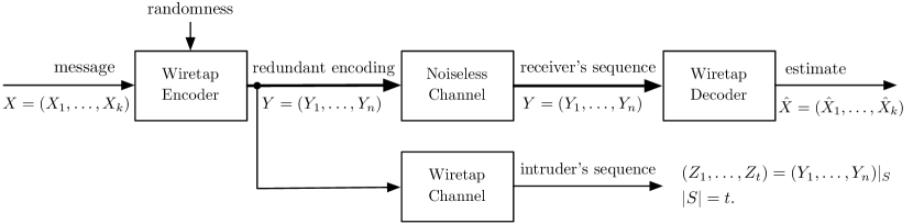
Figure 1: The Wiretap II Problem.

The system defined above is illustrated in Figure 1. The security of the system is defined by the following conditional entropy, known as “equivocation”:

$$\Delta:=\min_{S\colon|S|=t}H(X|Z).$$

When $\Delta=H(X)=m$, the intruder obtains no information about the transmitted message and we have perfect privacy in the system. Moreover, when $\Delta\to m$ as $m\to\infty$, we call the system asymptotically perfectly private. These two cases correspond to what is known in the literature as “strong secrecy”. A weaker requirement (known as “weak secrecy”) would be to have $m-\Delta=o(m)$.

Remark 3.1.

The assumption that $X$ is sampled from a uniformly random source should not be confused with the fact that Alice is transmitting one particular message to Bob that is fixed and known to her before the transmission. In this case, the randomness of $X$ in the model captures the a priori uncertainty about $X$ for the outside world, and in particular the intruder, but not the transmitter.

As an intuitive example, suppose that a random key is agreed upon between Alice and a trusted third party, and now Alice wishes to securely send her particular key to Bob over a wiretapped channel. Or, assume that Alice wishes to send an audio stream to Bob that is encoded and compressed using a conventional audio encoding method.

Furthermore, the particular choice of the distribution on $X$ as a uniformly random sequence will cause no loss of generality. If the distribution of $X$ is publicly known to be non-uniform, the transmitter can use a suitable source-coding scheme to compress the source to its entropy prior to the transmission, and ensure that from the intruder’s point of view, $X$ is uniformly distributed. On the other hand, it is also easy to see that if a protocol achieves perfect privacy under uniform message distribution, it achieves perfect privacy under any other distribution as well.

4 The Formal Model

The model that we will be considering in this chapter is motivated by the original wiretap channel problem but is more stringent in terms of its security requirements. In particular, instead of using Shannon entropy as a measure of uncertainty, we will rely on statistical indistinguishability which is a stronger measure that is more widely used in cryptography.

Definition 3.2.

Let $\Sigma$ be a set of size $q$, $m$ and $n$ be positive integers, and $\epsilon,\gamma>0$. A $(t,\epsilon,\gamma)_{q}$-resilient wiretap protocol of block length $n$ and message length $m$ is a pair of functions $E\colon\Sigma^{m}\times\{0,1\}^{r}\to\Sigma^{n}$ (the encoder) and $D\colon\Sigma^{n}\to\Sigma^{m}$ (the decoder) that are computable in time polynomial in $m$, such that

1. (Decodability) For all $x\in\Sigma^{m}$ and all $z\in\{0,1\}^{r}$ we have $D(E(x,z))=x$,

2. (Resiliency) Let ${X}\sim\mathcal{U}_{\Sigma^{m}}$, ${R}\sim\mathcal{U}_{r}$, and ${Y}=E(X,R)$. For a set $S\subseteq[n]$ and $w\in\Sigma^{|S|}$, let $\mathcal{X}_{S,w}$ denote the distribution of $X$ conditioned on the event $Y|_{S}=w$. Define the set of bad observations as

   $$B_{S}:=\{w\in\Sigma^{|S|}\mid{\mathsf{dist}}(\mathcal{X}_{S,w},\mathcal{U}_{\Sigma^{m}})>\epsilon\},$$

   where ${\mathsf{dist}}(\cdot,\cdot)$ denotes the statistical distance between two distributions. Then we require that for every $S\subseteq[n]$ of size at most $t$, $\Pr[Y|_{S}\in B_{S}]\leq\gamma$, where the probability is over the randomness of $X$ and $R$.

The encoding of a vector $x\in\Sigma^{k}$ is accomplished by choosing a vector $Z\in\{0,1\}^{r}$ uniformly at random, and calculating $E(x,Z)$. The quantities $R:=m/n$, $\epsilon$, and $\gamma$ are called the rate, the error, and the leakage of the protocol, respectively. Moreover, we call $\delta:=t/n$ the (relative) resilience of the protocol.

The decodability condition ensures that the functions $E$ and $D$ are a matching encoder/decoder pair, while the resiliency conditions ensures that the intruder learns almost nothing about the message from his observation.

In our definition, the imperfection of the protocol is captured by the two parameters $\epsilon$ and $\gamma$. When $\epsilon=\gamma=0$, the above definition coincides with the original wiretap channel problem for the case of perfect privacy.

When $\gamma=0$, we will have a worst-case guarantee, namely, that the intruder’s views of the message before and after his observation are statistically close, regardless of the outcome of the observation.

The protocol remains interesting even when $\gamma$ is positive but sufficiently small. When $\gamma>0$, a particular observation might potentially reveal to the intruder a lot of information about the message. However, a negligible $\gamma$ will ensure that such a bad event (or leakage) happens only with negligible probability.

All the constructions that we will study in this chapter achieve zero leakage (i.e., $\gamma=0$), except for the general result in Section 10.3 for which a nonzero leakage is inevitable.

The significance of zero-leakage protocols is that they assure adaptive resiliency in the weak sense introduced in [ref:DSS01] for exposure-resilient functions: if the intruder is given the encoded sequence as an oracle that he can adaptively query at up to $t$ coordinates (that is, the choice of each query may depend on the outcome of the previous queries), and is afterwards presented with a challenge which is either the original message or an independent uniformly chosen random string, he will not be able to distinguish between the two cases.

In general, it is straightforward to verify that our model can be used to solve the original wiretap II problem, with $\Delta\geq m(1-\epsilon-\gamma)$:

Lemma 3.3.

Suppose that $(E,D)$ is an encoder/decoder pair as in Definition 3.2. Then using $E$ and $D$ in the wiretap II problem attains an equivocation

$$\Delta\geq m(1-\epsilon-\gamma).$$

Proof.

Let $W:=Y|_{S}$ be the intruder’s observation, and denote by $W^{\prime}$ the set of good observations, namely,

$$W^{\prime}:=\{w\in\Sigma^{t}\colon{\mathsf{dist}}(\mathcal{X}_{S,w},\mathcal{U}_{\Sigma^{m}})\leq\epsilon\}.$$

Denote by $H(\cdot)$ the Shannon entropy in $d$-ary symbols. Then we will have

$$H(X|W) = \sum_{w\in\Sigma^{t}}\Pr(W=w)H(X|W=w)$$

$$\geq \sum_{w\in W^{\prime}}\Pr(W=w)H(X|W=w)$$

$$\stackrel{{\scriptstyle\mathrm{(a)}}}{{\geq}} \sum_{w\in W^{\prime}}\Pr(W=w)(1-\epsilon)m\stackrel{{\scriptstyle\mathrm{(b)}}}{{\geq}}(1-\gamma)(1-\epsilon)m\geq(1-\gamma-\epsilon)m.$$

The inequality $\mathrm{(a)}$ follows from the definition of $W^{\prime}$ combined with Proposition 3.30 in the appendix, and $\mathrm{(b)}$ by the definition of leakage parameter. ∎

Hence, we will achieve asymptotically perfect privacy when $\epsilon+\gamma=o(1/m)$. For all the protocols that we present in this chapter this quantity will be superpolynomially small; that is, smaller than $1/m^{c}$ for every positive constant $c$ (provided that $m$ is large enough).

5 Review of the Related Notions in Cryptography

There are several interrelated notions in the literature on Cryptography and Theoretical Computer Science that are also closely related to our definition of the wiretap protocol (Definition 3.2). These are resilient functions (RF) and almost perfect resilient functions (APRF), exposure-resilient functions (ERF), and all-or-nothing transforms (AONT) (cf. [ref:tResilient, ref:tResilient2, ref:Riv97, ref:Stinson, ref:FT00, ref:CDH, ref:KJS] and [ref:Dodis] for a comprehensive account of several important results in this area).

The notion of resilient functions was introduced in [ref:BBR85] (and also [ref:Vaz87] as the bit-extraction problem). A deterministic polynomial-time computable function $f\colon\{0,1\}^{n}\to\{0,1\}^{m}$ is called $t$-resilient if whenever any $t$ bits of the its input are arbitrarily chosen by an adversary and the rest of the bits are chosen uniformly at random, then the output distribution of the function is (close to) uniform. APRF is a stronger variation where the criterion for uniformity of the output distribution is defined with respect to the $\ell_{\infty}$ (i.e., point-wise distance of distributions) rather than $\ell_{1}$. This stronger requirement allows for an “adaptive security” of APRFs.

ERFs, introduced in [ref:CDH], are similar to resilient functions except that the entire input is chosen uniformly at random, and the view of the adversary from the output remains (close to) uniform even after observing any $t$ input bits of his choice.

ERFs and resilient functions are known to be useful in a scenario similar to the wiretap channel problem where the two parties aim to agree on any random string, for example a session key (Alice generates $x$ uniformly at random which she sends to Bob, and then they agree on the string $f(x)$). Here no control on the content of the message is required, and the only goal is that at the end of the protocol the two parties agree on any random string that is uniform even conditioned on the observations of the intruder. Hence, Definition 3.2 of a wiretap protocol is more stringent than that of resilient functions, since it requires the existence and efficient computability of the encoding function $E$ that provides a control over the content of the message.

Another closely related notion is that of all-or-nothing transforms, which was suggested in [ref:Riv97] for protection of block ciphers. A randomized polynomial-time computable function $f\colon\{0,1\}^{m}\to\{0,1\}^{n}$, $(m\leq n)$, is called a (statistical, non-adaptive, and secret-only) $t$-AONT with error $\epsilon$ if it is efficiently invertible and for every $S\subseteq[n]$ such that $|S|\leq t$, and all $x_{1},x_{2}\in\{0,1\}^{m}$ we have that the two distributions $f(x_{1})|_{S}$ and $f(x_{2})|_{S}$ are $\epsilon$-close.

An AONT with $\epsilon=0$ is called perfect. It is easy to see that perfectly private wiretap protocols are equivalent to perfect adaptive AONTs. It was shown in [ref:DSS01] that such functions can not exist (with positive, constant rate) when the adversary is allowed to observe more than half of the encoded bits. A similar result was obtained in [ref:tResilient] for the case of perfect linear RFs.

As pointed out in [ref:DSS01], AONTs can be used in the original scenario of Ozarow and Wyner’s wiretap channel problem. However, the best known constructions of AONTs can achieve rate-resilience trade-offs that are far from the information-theoretic optimum (see Figure 2).

While an AONT requires indistinguishability of intruder’s view for every fixed pair $(x_{1},x_{2})$ of messages, the relaxed notion of average-case AONT requires the expected distance of $f(x_{1})|_{S}$ and $f(x_{2})|_{S}$ to be at most $\epsilon$ for a uniform random message pair. Hence, for a negligible $\epsilon$, the distance will be negligible for all but a negligible fraction of message pairs. Up to a loss in parameters, wiretap protocols are equivalent to average case AONTs:

Lemma 3.4.

Let $(E,D)$ be an encoding/decoding pair for a $(t,\epsilon,\gamma)_{2}$-resilient wiretap protocol. Then $E$ is an average-case $t$-AONT with error at most $2(\epsilon+\gamma)$.

Conversely, an average-case $t$-AONT with error $\eta^{2}$ can be used as a $(t,\eta,\eta)$-resilient wiretap encoder.

Proof.

Consider a $(t,\epsilon,\gamma)_{2}$-resilient wiretap protocol as in Definition 3.2, and accordingly, let the random variable $Y=E(X,R)$ denote the encoding of $X$ with a random seed $R$. For a set $S\subseteq[n]$ of size at most $t$, denote by $W:=Y|_{S}$ the intruder’s observation.

The resiliency condition implies that, the set of bad observations $B_{S}$ has a probability mass of at most $\gamma$ and hence, the expected distance ${\mathsf{dist}}(X|W,X)$ taken over the distribution of $W$ is at most $\epsilon+\gamma$. Now we can apply Proposition 3.31 to the jointly distributed pair of random variables $(W,X)$, and conclude that the expected distance ${\mathsf{dist}}(W|X,W)$ over the distribution of $X$ (which is uniform) is at most $\epsilon+\gamma$. This implies that the encoder is an average-case $t$-AONT with error at most $2(\epsilon+\gamma)$.

Conversely, the same argument combined with Markov’s bound shows that an average-case $t$-AONT with error $\eta^{2}$ can be seen as $(t,\eta,\eta)$-resilient wiretap protocol. ∎

Note that the converse direction does not guarantee zero leakage, and hence, zero leakage wiretap protocols are in general stronger than average-case AONTs. An average-case to worst-case reduction for AONTs was shown in [ref:CDH] which, combined with the above lemma, can be used to show that any wiretap protocol can be used to construct an AONT (at the cost of a rate loss).

A simple universal transformation was proposed in [ref:CDH] to obtain an AONT from any ERF, by one-time padding the message with a random string obtained from the ERF. In particular, given an ERF $f\colon\{0,1\}^{n}\to\{0,1\}^{m}$, the AONT $g\colon\{0,1\}^{m}\to\{0,1\}^{m+n}$ is defined as $g(x):=(r,x+f(r))$, where $r\in\{0,1\}^{n}$ is chosen uniformly at random. Hence, the ERF is used to one-time pad the message with a random secret string.

This construction can also yield a wiretap protocol with zero leakage. However, it has the drawback of significantly weakening the rate-resilience trade-off. Namely, even if an information theoretically optimal ERF is used in this reduction, the resulting wiretap protocol will only achieve half the optimal rate (see Figure 2). This is because the one-time padding strategy necessarily requires a random seed that is at least as long as the message itself, even if the intruder is restricted to observe only a small fraction of the transmitted sequence. Hence the rate of the resulting AONT cannot exceed $1/2$, and it is not clear how to improve this universal transformation to obtain a worst-case AONT using a shorter seed.

The main focus of this chapter is on asymptotic trade-offs between the rate $R$ and the resilience $\delta$ of an asymptotically perfectly private wiretap protocol. For applications in cryptography, e.g., the context of ERFs or AONTs, it is typically assumed that the adversary learns all but a small number of the bits in the encoded sequence, and the incurred blow-up in the encoding is not as crucially important, as long as it remains within a reasonable range. On the other hand, as in this chapter we are motivated by the wiretap channel problem which is a communication problem, optimizing the transmission rate will be the most important concern for us. We will focus on the case where the fraction $\delta$ of the symbols observed by the intruder is an arbitrary constant below $1$, which is the most interesting range in our context. However, some of our constructions work for sub-constant $1-\delta$ as well.

Following [ref:Wyner2], it is easy to see that, for resilience $\delta$, an information-theoretic bound $R\leq 1-\delta+o(1)$ must hold. Lower bounds for $R$ in terms of $\delta$ have been studied by a number of researchers.

For the case of perfect privacy (where the equivocation $\Delta$ is equal to the message length $m$), Ozarow and Wyner [ref:Wyner2] give a construction of a wiretap protocol using linear error-correcting codes, and show that the existence of an $[n,k,d]_{q}$-code implies the existence of a perfectly private, $(d-1,0,0)_{q}$-resilient wiretap protocol with message length $k$ and block length $n$ (thus, rate $k/n$).

As a result, the so-called Gilbert-Varshamov bound on the rate-distance trade-offs of linear codes (see Chapter LABEL:chap:gv) implies that, asymptotically, $R\geq 1-h_{q}(\delta)$, where $h_{q}$ is the $q$-ary entropy function defined as

$$h_{q}(x):=x\log_{q}(q-1)-x\log_{q}(x)-(1-x)\log_{q}(1-x).$$

If $q\geq 49$ is a square, the bound can be further improved to $R\geq 1-\delta-1/(\sqrt{q}-1)$ using Goppa’s algebraic-geometric codes [gopp:81, tsvz:82]. In these protocols, the encoder can be seen as an adaptively secure, perfect AONTs and the decoder is an adaptive perfect RF.

Moving away from perfect to asymptotically perfect privacy, it was shown in [ref:KJS] that for any $\gamma>0$ there exist binary asymptotically perfectly private wiretap protocols with $R\geq 1-2\delta-\gamma$ and exponentially small error. This bound strictly improves the coding-theoretic bound of Ozarow and Wyner for the binary alphabet.

Figure 2: A comparison of the rate vs. resilience trade-offs achieved by the wiretap protocols for the binary alphabet (left) and larger alphabets (right, in this example of size $64$). $(1)$ Information-theoretic bound, attained by Theorem 3.25; $(2)$ The bound approached by [ref:KJS]; $(3)$ Protocol based on best non-explicit binary linear codes [gilbert, varshamov]; $(4)$ AONT construction of [ref:CDH], assuming that the underlying ERF is optimal; $(5)$ Random walk protocol of Corollary 3.19; $(6)$ Protocol based on the best known explicit [tsvz:82] and non-explicit [gilbert, varshamov] linear codes.

6 Symbol-Fixing and Affine Extractors

Two central notions for our constructions of wiretap protocols in this chapter are symbol-fixing and affine extractors. In this section, we introduce these notions, and study some basic constructions.

Definition 3.5.

A $d$-ary symbol-fixing source is an imperfect source of random symbols from an alphabet of size $d$, that may fix some bounded number of the symbols to unknown values. More precisely, an $(n,k)_{d}$ symbol-fixing source is the distribution of a random variable ${X}=({X}_{1},{X}_{2},\ldots,{X}_{n})\in\Sigma^{n}$, for some set $\Sigma$ of size $d$, in which at least $k$ of the coordinates (chosen arbitrarily) are uniformly and independently distributed on $\Sigma$ and the rest take deterministic values.

When $d=2$, we will have a binary symbol-fixing source, or simply a bit-fixing source. In this case $\Sigma=\{0,1\}$, and the subscript $d$ is dropped from the notation.

The min-entropy of a $(n,k)_{d}$ symbol-fixing source is $k\log_{2}d$ bits. For a $d$-ary source with $d\neq 2$, it is more convenient to talk about the $d$-ary entropy of the source, which is $k$ (in $d$-ary symbols).

Affine sources are natural generalizations of symbol-fixing sources when the alphabet size is a prime power.

Definition 3.6.

For a prime power $q$, an $(n,k)_{q}$ affine source is a distribution on $\mathds{F}_{q}^{n}$ that is uniformly supported on an affine translation of some $k$-dimensional subspace of $\mathds{F}_{q}^{n}$.

It is easy to see that the $q$-ary min-entropy of a $k$-dimensional affine source is $k$. Due to the restricted structure of symbol-fixing and affine sources, it is possible to construct seedless extractors for such sources:

Definition 3.7.

Let $\Sigma$ be a finite alphabet of size $d>1$. A function $f\colon\Sigma^{n}\to\Sigma^{m}$ is a (seedless) $(k,\epsilon)$-extractor for symbol-fixing (resp., affine) sources on $\Sigma^{n}$ if for every $(n,k)_{d}$ symbol-fixing (resp., affine) source $\mathcal{X}$, the distribution $E(\mathcal{X})$ is $\epsilon$-close to the uniform distribution $\mathcal{U}_{\Sigma^{m}}$. The extractor is called explicit if it is deterministic and polynomial-time computable.

We will shortly see simple constructions of zero-error, symbol-fixing and affine extractors using linear functions arising from good error-correcting codes. These extractors achieve the lowest possible error, but however are unable to extract the entire source entropy. Moreover, the affine extractor only works for a “restricted” class of affine sources. For unrestricted affine sources, there are by now various constructions of extractors in the literature. Here we review some notable examples that are most useful for the construction of wiretap protocols that we will discuss in this chapter.

Over large fields, the following affine extractor due to Gabizon and Raz extract almost the entire source entropy:

Theorem 3.8.

[ref:affine] There is a constant $q_{0}$ such that for any prime power field size $q$ and integers $n,k$ such that $q>\max\{q_{0},n^{20}\}$, there is an explicit affine $(k,\epsilon)$-extractor $f\colon\mathds{F}_{q}^{n}\to\mathds{F}_{q}^{k-1}$, where $\epsilon<q^{-1/21}$. ∎

In this construction, the field size has to be polynomially large in $n$. When the field size is small (in particular, constant), the task becomes much more challenging. The most challenging case thus corresponds to the binary field $\mathds{F}_{2}$, for which an explicit affine extractor was obtained, when the input entropy is a constant fraction of the input length, by Bourgain:

Theorem 3.9.

[ref:Bourgain] For every constant $0<\delta\leq 1$, there is an explicit affine extractor $\mathsf{AExt}\colon\mathds{F}_{2}^{n}\to\mathds{F}_{2}^{m}$ for min-entropy $\delta n$ with output length $m=\Omega(n)$ and error at most $2^{-\Omega(m)}$. ∎

Bourgain’s construction was recently simplified, improved, and extended to work for arbitrary prime fields by Yehudayoff [ref:Yeh09].

An “intermediate” trade-off is recently obtained by DeVos and Gabizon [ref:DG10], albeit with a short output length. This explicit construction extracts one unbiased bit from any $(n,k)_{q}$ affine source provided that, for $d:=5n/k$, we have $q>2d^{2}$ and the characteristic of the field is larger than $d$.

6.1 Symbol-Fixing Extractors from Linear Codes

The simple theorem below states that linear error-correcting codes can be used to obtain symbol-fixing extractors with zero error.

Theorem 3.10.

Let $\mathcal{C}$ be an $[n,{\tilde{k}},d]_{q}$ code over $\mathds{F}_{q}$ and $G$ be a ${\tilde{k}}\times n$ generator matrix of $\mathcal{C}$. Then, the function $E\colon\mathds{F}_{q}^{n}\to\mathds{F}_{q}^{\tilde{k}}$ defined as $E(x):=Gx^{\top}$ is an $(n-d+1,0)$-extractor for symbol-fixing sources over $\mathds{F}_{q}$.

Conversely, if a linear function $E\colon\mathds{F}_{q}^{n}\to\mathds{F}_{q}^{\tilde{k}}$ is an $(n-d+1,0)$-extractor for symbol-fixing sources over $\mathds{F}_{q}$, it corresponds to a generator matrix of an $[n,{\tilde{k}},d]_{q}$ code.

Proof.

Let $\mathcal{X}$ be a symbol-fixing source with a set $S\subseteq[n]$ of fixed coordinates, where $|S|=d-1$, and define $\bar{S}:=[n]\setminus S$. Observe that, by the Singleton bound, we must have $|\bar{S}|=n-d+1\geq{\tilde{k}}$.

The submatrix of $G$ obtained by removing the columns picked by $S$ must have rank ${\tilde{k}}$. Since otherwise, the left kernel of this submatrix would be nonzero, meaning that $\mathcal{C}$ has a nonzero codeword that consists of entirely zeros at the $d-1$ positions picked by $S$, contradicting the assumption that the minimum distance of $\mathcal{C}$ is $d$. Therefore, the distribution $E(\mathcal{X})$ is supported on a ${\tilde{k}}$-dimensional affine space on $\mathds{F}_{q}^{\tilde{k}}$, meaning that this distribution is uniform.

The converse is straightforward by following the same argument. ∎

If the field size is large enough; e.g., $q\geq n$, then one can pick $\mathcal{C}$ in the above theorem to be an MDS code (in particular, a Reed-Solomon code) to obtain a $(k,0)$-extractor for all symbol-fixing sources of entropy $k$ with optimal output length $k$. However, for a fixed $q$, negative results on the rate-distance trade-offs of codes (e.g., Hamming, MRRW, and Plotkin bounds) assert that this construction of extractors must inevitably lose some fraction of the entropy of the source. Moreover, the construction would at best be able to extract some constant fraction of the source entropy only if the entropy of the source (in $q$-ary symbols) is above $n/q$.

6.2 Restricted Affine Extractors from Rank-Metric Codes

In Section 10, we will see that affine extractors can be used to construct wiretap schemes for models that are more general than the original Wiretap II problem, e.g., when the direct channel is noisy. For these applications, the extractor needs to additionally have a nice structure that is in particular offered by linear functions.

An obvious observation is that a nontrivial affine extractor cannot be a linear function. Indeed, a linear function $f(x):=\langle\alpha,x\rangle+\beta$, where $\alpha,\beta,x\in\mathds{F}_{q}^{n}$, is constant on the $(n-1)$-dimensional orthogonal subspace of $\alpha$, and thus, fails to be an extractor for even $(n-1)$-dimensional affine spaces. However, in this section we will see that linear affine extractors can be constructed if the affine source is known to be described by a set of linear constraints whose coefficients lie on a small sub-field of the underlying field. Such restricted extractors turn out to be sufficient for some of the applications that we will consider.

Let $Q$ be a prime power. Same as linear codes, an affine subspace on $\mathds{F}_{Q}^{n}$ can be represented by a generator matrix, or parity-check matrix and a constant shift. That is, a $k$-dimensional affine subspace $A\subseteq\mathds{F}_{Q}^{n}$ can be described as the image of a linear mapping

$$A:=\{xG+\beta\colon x\in\mathds{F}_{Q}^{k}\},$$

where $G$ is a $k\times n$ generator matrix of rank $k$ over $\mathds{F}_{Q}$, and $\beta\in\mathds{F}_{Q}^{n}$ is a fixed vector. Alternatively, $A$ can be expressed as the translated null-space of a linear mapping

$$A:=\{x+\beta\in\mathds{F}_{Q}^{n}\colon Hx^{\top}=0\},$$

for an $(n-k)\times n$ parity check matrix of rank $n-k$ over $\mathds{F}_{Q}$.

Observe that a symbol-fixing source over $\mathds{F}_{q}$ with $q$-ary min-entropy $k$ can be seen as a $k$-dimensional affine source with a generator matrix of the form $[I\mid\mathbf{0}]\cdot P$, where $I$ is the $k\times k$ identity matrix, $\mathbf{0}$ denotes the $k\times(n-k)$ all-zeros matrix, and $P$ is a permutation matrix. Recall that from Theorem 3.10 we know that for this restricted type of affine sources linear extractors exist. In this section we generalize this idea.

Suppose that $Q=q^{m}$ for a prime power $q$ so that $\mathds{F}_{Q}$ can be regarded as a degree $m$ extension of $\mathds{F}_{q}$ (and isomorphic to $\mathds{F}_{q^{m}}$). Let $A$ be an affine source over $\mathds{F}_{Q}^{n}$. We will call the affine source $\mathds{F}_{q}$-restricted if its support can be represented by a generator matrix (or equivalently, a parity check matrix) over $\mathds{F}_{q}$.

In this section we introduce an affine extractor that is $\mathds{F}_{Q}$-linear and, assuming that $m$ is sufficiently large, extracts from $\mathds{F}_{q}$-restricted affine sources. The construction of the extractor is similar to Theorem 3.10, except that instead of an error-correcting code defined over the Hamming metric, we will use rank-metric codes.

Consider the function ${\mathsf{rdist}}\colon\mathds{F}_{q}^{m\times n}\times\mathds{F}_{q}^{m\times n}\to\mathds{Z}$, where $\mathds{F}_{q}^{m\times n}$ denotes the set of $m\times n$ matrices over $\mathds{F}_{q}$, defined as ${\mathsf{rdist}}(A,B):={\mathsf{rank}}_{q}(A-B)$, where ${\mathsf{rank}}_{q}$ is the matrix rank over $\mathds{F}_{q}$. It is straightforward to see that ${\mathsf{rdist}}$ is a metric.

The usual notion of error-correcting codes defined under the Hamming metric can be naturally extended to the rank metric. In particular, a rank-metric code $\mathcal{C}$ can be defined as a set of $m\times n$ matrices (known as codewords), whose minimum distance is the minimum rank distance between pairs of codewords.

For $Q:=q^{m}$, there is a natural correspondence between $m\times n$ matrices over $\mathds{F}_{q}$ and vectors of length $n$ over $\mathds{F}_{Q}$. Consider an isomorphism $\varphi\colon\mathds{F}_{Q}\to\mathds{F}_{q}^{m}$ between $\mathds{F}_{Q}$ and $\mathds{F}_{q}^{m}$ which maps elements of $\mathds{F}_{Q}$ to column vectors of length $m$ over $\mathds{F}_{q}$. Then one can define a mapping $\Phi\colon\mathds{F}_{Q}^{n}\to\mathds{F}_{q}^{m\times n}$ defined as

$$\Phi(x_{1},\ldots,x_{n}):=[\varphi(x_{1})\mid\cdots\mid\varphi(x_{n})]$$

to put the elements of $\mathds{F}_{Q}^{n}$ in one-to-one correspondence with $m\times n$ matrices over $\mathds{F}_{q}$.

A particular class of rank-metric codes are linear ones. Suppose that $\mathcal{C}$ is a linear $[n,{\tilde{k}},\tilde{d}]_{Q}$ code over $\mathds{F}_{Q}$. Then, using $\Phi(\cdot)$, $\mathcal{C}$ can be regarded as a rank-metric code of dimension ${\tilde{k}}$ over $\mathds{F}_{q}^{m\times n}$. In symbols, we will denote such a linear ${\tilde{k}}$-dimensional rank-metric code as an $[[n,{\tilde{k}},d]]_{q^{m}}$ code, where $d$ is the minimum rank-distance of the code. The rank-distance of a linear rank-metric code turns out to be equal to the minimum rank of its nonzero codewords and obviously, one must have $d\leq\tilde{d}$. However, the Hamming distance of $\mathcal{C}$ might turn out to be much larger than its rank distance when regarded as a rank-metric code. In particular, $d\leq m$, and thus, $d$ must be strictly smaller than $\tilde{d}$ when the degree $m$ of the field extension is less than $\tilde{d}$.

A counterpart of the Singleton bound in the rank-metric states that, for any $[[n,{\tilde{k}},d]]_{q^{m}}$ code, one must have $d\leq n-{\tilde{k}}+1$. Rank-metric codes that attain equality exist and are called maximum rank distance (MRD) codes. A class of linear rank-metric codes known as Gabidulin codes [ref:Gab85] are MRD and can be thought of as the counterpart of Reed-Solomon codes in the rank metric. In particular, the codewords of a Gabidulin code, seen as vectors over the extension field, are evaluation vectors of bounded-degree linearized polynomials rather than arbitrary polynomials as in the case of Reed-Solomon codes. These codes are defined for any choice of $n,{\tilde{k}},q,m$ as long as $m\geq n$ and ${\tilde{k}}\leq n$.

The following is an extension of Theorem 3.10 to restricted affine sources.

Theorem 3.11.

Let $\mathcal{C}$ be an $[[n,{\tilde{k}},d]]_{q^{m}}$ code defined from a code over $\mathds{F}_{Q}$ (where $Q:=q^{m}$) with a generator matrix $G\in\mathds{F}_{Q}^{{\tilde{k}}\times n}$. Then the function $E\colon\mathds{F}_{Q}^{n}\to\mathds{F}_{Q}^{\tilde{k}}$ defined as $E(x):=Gx^{\top}$ is an $(n-d+1,0)$-extractor for $\mathds{F}_{q}$-restricted affine sources over $\mathds{F}_{Q}$.

Conversely, if a linear function $E\colon\mathds{F}_{Q}^{n}\to\mathds{F}_{Q}^{\tilde{k}}$ is an $(n-d+1,0)$-extractor for all $\mathds{F}_{q}$-restricted affine sources over $\mathds{F}_{Q}$, it corresponds to a generator matrix of an $[[n,{\tilde{k}},d]]_{q^{m}}$ code.

Proof.

Consider a restricted affine source $\mathcal{X}$ uniformly supported on an affine subspace of dimension $n-d+1$

$$X:=\{xA+\beta\colon x\in\mathds{F}_{Q}^{n-d+1}\},$$

where $A\in\mathds{F}_{q}^{(n-d+1)\times n}$ has rank $n-d+1$, and $\beta\in\mathds{F}_{Q}^{n}$ is a fixed translation. Note that ${\tilde{k}}\leq n-d+1$ by the Singleton bound for rank-metric codes.

The output of the extractor is thus uniformly supported on the affine subspace

$$B:=\{GA^{\top}x^{\top}+G\beta^{\top}\colon x\in\mathds{F}_{Q}^{n-d+1}\}\subseteq\mathds{F}_{Q}^{\tilde{k}}.$$

Note that $GA^{\top}\in\mathds{F}_{Q}^{{\tilde{k}}\times(n-d+1)}$. Our goal is to show that the dimension of $B$ is equal to ${\tilde{k}}$. Suppose not, then we must have ${\mathsf{rank}}_{Q}(GA^{\top})<{\tilde{k}}$. In particular, there is a nonzero $y\in\mathds{F}_{Q}^{\tilde{k}}$ such that $yGA^{\top}=0$.

Let $Y:=\Phi(yG)\in\mathds{F}_{q}^{m\times n}$, where $\Phi(\cdot)$ is the isomorphism that maps codewords of $\mathcal{C}$ to their matrix form over $\mathds{F}_{q}$. By the distance of $\mathcal{C}$, we know that ${\mathsf{rank}}_{q}(Y)\geq d$. Since $m\geq d$, this means that $Y$ has at least $d$ linearly independent rows. On the other hand, we know that the matrix $YA^{\top}\in\mathds{F}_{q}^{{\tilde{k}}\times(n-d+1)}$ is the zero matrix. Therefore, $Y$ has $d$ independent rows (each in $\mathds{F}_{q}^{n}$) that are all orthogonal to the $n-d+1$ independent rows of $A$. Since $d+(n-d+1)>n$, this is a contradiction.

Therefore, the dimension of $B$ is exactly ${\tilde{k}}$, meaning that the output distribution of the extractor is indeed uniform. The converse is straightforward by following a similar line of argument. ∎

Thus, in particular, we see that generator matrices of MRD codes can be used to construct linear extractors for restricted affine sources that extract the entire source entropy with zero error. This is possible provided that the field size is large enough compared to the field size required to describe the generator matrix of the affine source. Using Gabidulin’s rank metric codes, we immediately obtain the following corollary of Theorem 3.11:

Corollary 3.12.

Let $q$ be a prime power. Then for every positive integer $n$, $k\leq n$, and $Q:=q^{n}$, there is a linear function $f\colon\mathds{F}_{Q}^{n}\to\mathds{F}_{Q}^{k}$ that is a $(k,0)$-extractor for $\mathds{F}_{q}$-restricted affine sources over $\mathds{F}_{Q}$. ∎

It can be shown using similar proofs that if, in Theorems 3.10 and 3.11, a parity check matrix of the code is used instead of a generator matrix, the resulting linear function would become a lossless $(d-1,0)$-condenser rather than an extractor. This is in fact part of a more general “duality” phenomenon that is discussed in Section LABEL:sec:dualityAffine.

7 Inverting Extractors

In this section we will introduce the notion of invertible extractors and its connection with wiretap protocols. Later we will use this connection to construct wiretap protocols with good rate-resilience trade-offs.

Definition 3.13.

Let $\Sigma$ be a finite alphabet and $f$ be a mapping from $\Sigma^{n}$ to $\Sigma^{m}$. For $\gamma\geq 0$, a function $A\colon\Sigma^{m}\times\{0,1\}^{r}\to\Sigma^{n}$ is called a $\gamma$-inverter for $f$ if the following conditions hold:

1. (Inversion) Given $x\in\Sigma^{m}$ such that $f^{-1}(x)$ is nonempty, for every $z\in\{0,1\}^{r}$ we have $f(A(x,z))=x$.

2. (Uniformity) $A(\mathcal{U}_{\Sigma^{m}},\mathcal{U}_{r})\sim_{\gamma}\mathcal{U}_{\Sigma^{n}}$.

A $\gamma$-inverter is called efficient if there is a randomized algorithm that runs in worst case polynomial time and, given $x\in\Sigma^{m}$ and $z$ as a random seed, computes $A(x,z)$. We call a mapping $\gamma$-invertible if it has an efficient $\gamma$-inverter, and drop the prefix $\gamma$ from the notation when it is zero.

The parameter $r$ in the above definition captures the amount of random bits that the inverter (seen as a randomized algorithm) needs to receive. For our applications, no particular care is needed to optimize this parameter and, as long as $r$ is polynomially bounded in $n$, it is generally ignored.

Remark 3.14.

If a function $f$ maps the uniform distribution to a distribution that is $\epsilon$-close to uniform (as is the case for all extractors), then any randomized mapping that maps its input $x$ to a distribution that is $\gamma$-close to the uniform distribution on $f^{-1}(x)$ is easily seen to be an $(\epsilon+\gamma)$-inverter for $f$. In some situations designing such a function might be easier than directly following the above definition.

The idea of random pre-image sampling was proposed in [ref:DSS01] for construction of adaptive AONTs from APRFs. However, they ignored the efficiency of the inversion, as their goal was to show the existence of (not necessarily efficient) information-theoretically optimal adaptive AONTs. Moreover, the strong notion of APRF and a perfectly uniform sampler is necessary for their construction of AONTs. As wiretap protocols are weaker than (worst-case) AONTs, they can be constructed from slightly imperfect inverters as shown by the following lemma.

Lemma 3.15.

Let $\Sigma$ be an alphabet of size $q>1$ and $f\colon\Sigma^{n}\to\Sigma^{m}$ be a $(\gamma^{2}/2)$-invertible $q$-ary $(k,\epsilon)$ symbol-fixing extractor. Then, $f$ and its inverter can be seen as a decoder/encoder pair for an $(n-k,\epsilon+\gamma,\gamma)_{q}$-resilient wiretap protocol with block length $n$ and message length $m$.

Proof.

Let $E$ and $D$ denote the wiretap encoder and decoder, respectively. Hence, $E$ is the $(\gamma^{2}/2)$-inverter for $f$, and $D$ is the extractor $f$ itself. From the definition of the inverter, for every $x\in\Sigma^{m}$ and every random seed $r$, we have $D(E(x,r))=x$. Hence it is sufficient to show that the pair satisfies the resiliency condition.

Let the random variable $X$ be uniformly distributed on $\Sigma^{m}$ and the seed $R\in\{0,1\}^{r}$ be chosen uniformly at random. Denote the encoding of $X$ by $Y:=E(X,R)$. Fix any $S\subseteq[n]$ of size at most $n-k$.

For every $w\in\Sigma^{|S|}$, let $Y_{w}$ denote the set $\{y\in\Sigma^{n}\colon(y|_{S})=w\}$. Note that the sets $Y_{w}$ partition the space $\Sigma^{n}$ into $|\Sigma|^{|S|}$ disjoint sets.

Let $\mathcal{Y}$ and $\mathcal{Y}_{S}$ denote the distribution of $Y$ and $Y|_{S}$, respectively. The inverter guarantees that $\mathcal{Y}$ is $(\gamma^{2}/2)$-close to uniform. Applying Proposition 3.32, we get that

$$\sum_{w\in\Sigma^{|S|}}\Pr[(Y|_{S})=w]\cdot{\mathsf{dist}}((\mathcal{Y}|Y_{w}),\mathcal{U}_{Y_{w}})\leq\gamma^{2}.$$

The left hand side is the expectation of ${\mathsf{dist}}((\mathcal{Y}|Y_{w}),\mathcal{U}_{Y_{w}})$. Denote by $W$ the set of all bad outcomes of $Y|_{S}$, i.e.,

$$W:=\{w\in\Sigma^{|S|}\mid{\mathsf{dist}}((\mathcal{Y}|Y_{w}),\mathcal{U}_{Y_{w}})>\gamma\}.$$

By Markov’s inequality, we conclude that

$$\Pr[(Y|_{S})\in W]\leq\gamma.$$

For every $w\in W$, the distribution of $Y$ conditioned on the event $(Y|_{S})=w$ is $\gamma$-close to a symbol-fixing source with $n-|S|\geq k$ random symbols. The fact that $D$ is a symbol-fixing extractor for this entropy and Proposition 3.33 imply that, for any such $w$, the conditional distribution of $D(Y)|(Y|_{S}=w)$ is $(\gamma+\epsilon)$-close to uniform. Hence with probability at least $1-\gamma$ the distribution of $X$ conditioned on the outcome of $Y|_{S}$ is $(\gamma+\epsilon)$-close to uniform. This ensures the resiliency of the protocol. ∎

By combining Lemma 3.15 and Theorem 3.10 using a Reed-Solomon code, we can obtain a perfectly private, rate-optimal, wiretap protocol for the Wiretap II problem over large alphabets (namely, $q\geq n$), and recover the original result of Ozarow and Wyner [ref:Wyner2]:

Corollary 3.16.

For every positive integer $n$, prime power $q\geq n$, and $\delta\in[0,1)$, there is a $(\delta n,0,0)_{q}$-resilient wiretap protocol with block length $n$ and rate $1-\delta$ that attains perfect privacy. ∎

8 A Wiretap Protocol Based on Random Walks

In this section we describe a wiretap protocol that achieves a rate $R$ within a constant fraction of the information theoretically optimal value $1-\delta$ (the constant depending on the alphabet size).

To achieve our result, we will modify the symbol-fixing extractor of Kamp and Zuckerman [ref:KZ], that is based on random walks on expander graphs, to make it efficiently invertible without affecting its extraction properties, and then apply Lemma 3.15 above to obtain the desired wiretap protocol.

Before we proceed, let us briefly review some basic notions and facts related to expander graphs. For a detailed review of the theory of expander graphs, refer to the excellent survey by Hoory, Linial and Wigderson [HLW06], and books [ref:MR, ref:MU].

We will be working with directed regular expander graphs that are obtained from undirected graphs by replacing each undirected edge with two directed edges in opposite directions. Let $G=(V,E)$ be a $d$-regular graph. Then a labeling of the edges of $G$ is a function $L\colon V\times[d]\to V$ such that for every $u\in V$ and $t\in[d]$, the edge $(u,L(u,t))$ is in $E$. The labeling is consistent if whenever $L(u,t)=L(v,t)$, then $u=v$. Note that the natural labeling of a Cayley graph (cf. [HLW06]) is in fact consistent.

A family of $d$-regular graphs is an infinite set of $d$-regular graphs such that for every $N\in\mathds{N}$, the set contains a graph with at least $N$ vertices. For a parameter $c\geq 1$, we will call a family $c$-dense if there is an $N_{0}\in\mathds{N}$ such that, for every $N\geq N_{0}$, the family has a graph with at least $N$ and at most $cN$ vertices. We call a family of graphs constructible if all the graphs in the family have a consistent labeling that is efficiently computable. That is, there is a uniform, polynomial-time algorithm that, given $N\in\mathds{N}$ and $i\in[N],j\in[d]$, outputs the label of the $j$th neighbor of the $i$th vertex, under a consistent labeling, in the graph in the family that has $N$ vertices (provided that it exists).

Let $A$ denote the normalized adjacency matrix of a $d$-regular graph $G$ (that is, the adjacency matrix with all the entries divided by $d$). We denote by $\lambda_{G}$ the second largest eigenvalue of $A$ in absolute value. The spectral gap of $G$ is given by $1-\lambda_{G}$. Starting from a probability distribution $p$ on the set of vertices, represented as a real vector with coordinates index by the vertex set, performing a single-step random walk on $G$ leads to the distribution defined by $pA$. The following is a well known lemma on the convergence of the distributions resulting from random walks (see [ref:Lovasz] for a proof):

Lemma 3.17.

Let $G=(V,E)$ be a $d$-regular undirected graph, and $A$ be its normalized adjacency matrix. Then for any probability vector $p$, we have

$$\|pA-\mathcal{U}_{V}\|_{2}\leq\lambda_{G}\|p-\mathcal{U}_{V}\|_{2},$$

where $\|\cdot\|_{2}$ denotes the $\ell_{2}$ norm. ∎

The extractor of Kamp and Zuckerman [ref:KZ] starts with a fixed vertex in a large expander graph and interprets the input as the description of a walk on the graph. Then it outputs the label of the vertex reached at the end of the walk. Notice that a direct approach to invert this function will amount to sampling a path of a particular length between a pair of vertices in the graph, uniformly among all the possibilities, which might be a difficult problem for good families of expander graphs. We work around this problem by choosing the starting point of the walk from the input. The price that we pay by doing so is a slightly larger error compared to the original construction of Kamp and Zuckerman that is, asymptotically, of little significance. In particular we show the following:

Theorem 3.18.

Let $G$ be a constructible $d$-regular graph with $d^{m}$ vertices and second largest eigenvalue $\lambda_{G}\geq 1/\sqrt{d}$. Then there exists an explicit invertible $(k,2^{s/2})_{d}$ symbol-fixing extractor $\mathsf{SFExt}\colon[d]^{n}\to[d]^{m}$, such that

$$s:=\left\{\begin{array}[]{ll}m\log d+k\log\lambda_{G}^{2}&\text{if $k\leq n-m$,}\\ (n-k)\log d+(n-m)\log\lambda_{G}^{2}&\text{if $k>n-m$.}\\ \end{array}\right.$$

Proof.

We first describe the extractor and its inverse. Given an input $(v,w)\in[d]^{m}\times[d]^{n-m},$ the function $\mathsf{SFExt}$ interprets $v$ as a vertex of $G$ and $w$ as the description of a walk starting from $v$. The output is the index of the vertex reached at the end of the walk. Figure 3 depicts the procedure. The $4$-regular graph shown in this toy example has $8$ vertices labeled with binary sequences of length $3$. Edges of the graph are consistently labeled at both endpoints with the set of labels $\{1,2,3,4\}$. The input sequence $(0,1,0\mid 2,3,4,2,4$) shown below the graph describes a walk starting from the vertex $010$ and following the path shown by the solid arrows. The output of the extractor is the label of the final vertex $011$.

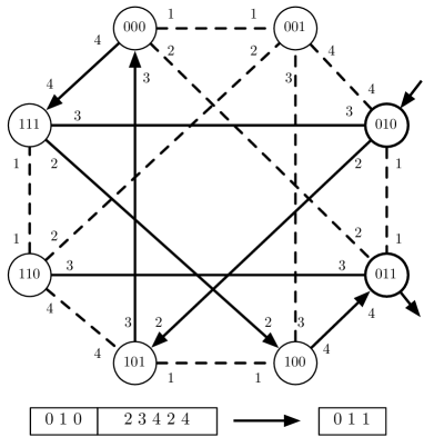
Figure 3: The random-walk symbol-fixing extractor.

The inverter $\mathsf{Inv}$ works as follows: Given $x\in[d]^{m}$, $x$ is interpreted as a vertex of $G$. Then $\mathsf{Inv}$ picks $W\in[d]^{n-m}$ uniformly at random. Let $V$ be the vertex starting from which the walk described by $W$ ends up in $x$. The inverter outputs $(V,W)$. It is easy to verify that $\mathsf{Inv}$ satisfies the properties of a $0$-inverter.

Now we show that $\mathsf{SFExt}$ is an extractor with the given parameters. We will follow the same line of argument as in the original proof of Kamp and Zuckerman. Let $(x,w)\in[d]^{m}\times[d]^{n-m}$ be a vector sampled from an $(n,k)_{d}$ symbol-fixing source, and let $u:=\mathsf{SFExt}(x,w)$. Recall that $u$ can be seen as the vertex of $G$ reached at the end of the walk described by $w$ starting from $x$. Let $p_{i}$ denote the probability vector corresponding to the walk right after the $i$th step, for $i=0,\ldots,n-m$, and denote by $p$ the uniform probability vector on the vertices of $G$. Our goal is to bound the error $\epsilon$ of the extractor, which is half the $\ell_{1}$ norm of $p_{n-m}-p$.

Suppose that $x$ contains $k_{1}$ random symbols and the remaining $k_{2}:=k-k_{1}$ random symbols are in $w$. Then $p_{0}$ has the value $d^{-k_{1}}$ at $d^{k_{1}}$ of the coordinates and zeros elsewhere, hence

$$\|p_{0}-p\|_{2}^{2}=d^{k_{1}}(d^{-k_{1}}-d^{-m})^{2}+(d^{m}-d^{k_{1}})d^{-2m}=d^{-k_{1}}-d^{-m}\leq d^{-k_{1}}.$$

Now for each $i\in[n-m]$, if the $i$th step of the walk corresponds to a random symbol in $w$ the $\ell_{2}$ distance is multiplied by $\lambda_{G}$ by Lemma 3.17. Otherwise the distance remains the same due to the fact that the labeling of $G$ is consistent. Hence we obtain $\|p_{n-m}-p\|_{2}^{2}\leq d^{-k_{1}}\lambda_{G}^{2k_{2}}$. Translating this into the $\ell_{1}$ norm by using the Cauchy-Schwarz inequality, we obtain $\epsilon$, namely,

$$\epsilon\leq\frac{1}{2}d^{(m-k_{1})/2}\lambda_{G}^{k_{2}}<2^{((m-k_{1})\log d+k_{2}\log\lambda_{G}^{2})/2}.$$

By our assumption, $\lambda_{G}\geq 1/\sqrt{d}$. Hence, everything but $k_{1}$ and $k_{2}$ being fixed, the above bound is maximized when $k_{1}$ is minimized. When $k\leq n-m$, this corresponds to the case $k_{1}=0$, and otherwise to the case $k_{1}=k-n+m$. This gives us the desired upper bound on $\epsilon$. ∎

Combining this with Lemma 3.15 and setting up the the right asymptotic parameters, we obtain our protocol for the wiretap channel problem.

Corollary 3.19.

Let $\delta\in[0,1)$ and $\gamma>0$ be arbitrary constants, and suppose that there is a constructible family of $d$-regular expander graphs with spectral gap at least $1-\lambda$ that is $c$-dense, for constants $\lambda<1$ and $c\geq 1$.

Then, for every large enough $n$, there is a $(\delta n,2^{-\Omega(n)},0)_{d}$-resilient wiretap protocol with block length $n$ and rate

$$R=\max\{\alpha(1-\delta),1-\delta/\alpha\}-\gamma,$$

where $\alpha:=-\log_{d}\lambda^{2}$.

Proof.

For the case $c=1$ we use Lemma 3.15 with the extractor $\mathsf{SFExt}$ of Theorem 3.18 and its inverse. Every infinite family of graphs must satisfy $\lambda\geq 2\sqrt{d-1}/d$ [ref:nilli], and in particular we have $\lambda\geq 1/\sqrt{d}$, as required by Theorem 3.18. We choose the parameters $k:=(1-\delta)n$ and $m:=n(\max\{\alpha(1-\delta),1-\delta/\alpha\}-\gamma)$, which gives $s=-\Omega(n)$, and hence, exponentially small error. The case $c>1$ is similar, but involves technicalities for dealing with lack of graphs of arbitrary size in the family. We will elaborate on this in Appendix 3.A. ∎

Using explicit constructions of Ramanujan graphs that achieve

$$\lambda\leq 2\sqrt{d-1}/d$$

when $d-1$ is a prime power [ref:ramanujan1, ref:ramanujan2, ref:pizer], one can obtain $\alpha\geq 1-2/\log d$, which can be made arbitrarily close to one (hence, making the protocol arbitrarily close to the optimal bound) by choosing a suitable alphabet size that does not depend on $n$. Namely, we have the following result:

Corollary 3.20.

Let $\delta\in[0,1)$ and $\gamma>0$ be arbitrary constants. Then, there is a positive integer $d$ only depending on $\gamma$ such that the following holds: For every large enough $n$, there is a $(\delta n,2^{-\Omega(n)},0)_{d}$-resilient wiretap protocol with block length $n$ and rate at least $1-\delta-\gamma$. ∎

9 Invertible Affine Extractors and Asymptotically Optimal Wiretap Protocols

In this section we will construct a black box transformation for making certain seedless extractors invertible. The method is described in detail for affine extractors, and leads to wiretap protocols with asymptotically optimal rate-resilience trade-offs. Being based on affine extractors, these protocols are only defined for prime power alphabet sizes. On the other hand, the random-walk based protocol discussed in Section 8 can be potentially instantiated for an arbitrary alphabet size, though achieving asymptotically sub-optimal parameters (and a positive rate only for an alphabet of size $3$ or more).

Modulo some minor differences, the construction can be simply described as follows: A seedless affine extractor is first used to extract a small number of uniform random bits from the source, and the resulting sequence is then used as the seed for a seeded extractor that extracts almost the entire entropy of the source.

Of course, seeded extractors in general are not guaranteed to work if (as in the above construction) their seed is not independent from the source. However, as observed by Gabizon and Raz [ref:affine], a linear seeded extractor can extract from an affine source if the seed is the outcome of an affine extractor on the source. This idea was formalized in a more general setting by Shaltiel [ref:mileage].

Shaltiel’s result gives a general framework for transforming any seedless extractor (for a family of sources satisfying a certain closedness condition) with short output length to one with an almost optimal output length. The construction uses the imperfect seedless extractor to extract a small number of uniform random bits from the source, and will then use the resulting sequence as the seed for a seeded extractor to extract more random bits from the source. For a suitable choice of the seeded extractor, one can use this construction to extract almost all min-entropy of the source.

The closedness condition needed for this result to work for a family $\mathcal{C}$ of sources is that, letting $E(x,s)$ denote the seeded extractor with seed $s$, for every $\mathcal{X}\in\mathcal{C}$ and every fixed $s$ and $y$, the distribution $(\mathcal{X}|E(\mathcal{X},s)=y)$ belongs to $\mathcal{C}$. If $E$ is a linear function for every fixed $s$, the result will be available for affine sources (since we are imposing a linear constraint on an affine source, it remains an affine source). A more precise statement of Shaltiel’s main result is the following:

Theorem 3.21.

[ref:mileage] Let $\mathcal{C}$ be a class of distributions on $\mathds{F}_{2}^{n}$ and $F\colon\mathds{F}_{2}^{n}\to\mathds{F}_{2}^{t}$ be an extractor for $\mathcal{C}$ with error $\epsilon$. Let $E\colon\mathds{F}_{2}^{n}\times\mathds{F}_{2}^{t}\to\mathds{F}_{2}^{m}$ be a function for which $\mathcal{C}$ satisfies the closedness condition above. Then for every $\mathcal{X}\in\mathcal{C}$, $E(\mathcal{X},F(\mathcal{X}))\sim_{\epsilon\cdot 2^{t+3}}E(\mathcal{X},\mathcal{U}_{t})$. ∎

Recall that a seeded extractor is called linear if it is a linear function for every fixed choice of the seed, and that this condition is satisfied by Trevisan’s extractor [ref:Tre]. For our construction, we will use the following theorem implied by the improvement of this extractor due to Raz, Reingold and Vadhan (Theorem 2.20):

Theorem 3.22.

[ref:RRV] There is an explicit strong linear seeded $(k,\epsilon)$-extractor $\mathsf{Ext}\colon\mathds{F}_{2}^{n}\times\mathds{F}_{2}^{d}\to\mathds{F}_{2}^{m}$ with $d=O(\log^{3}(n/\epsilon))$ and $m=k-O(d)$. ∎

Remark 3.23.

We note that our arguments would identically work for any other linear seeded extractor as well, for instance those constructed in [ref:RMExtractor, ref:SU]. However, the most crucial parameter in our application is the output length of the extractor, being closely related to the rate of the wiretap protocols we obtain. Among the constructions we are aware of, the result quoted in Theorem 3.22 is the best in this regard. Moreover, an affine seeded extractor with better parameters is constructed by Gabizon and Raz [ref:affine], but it requires a large alphabet size to work.

Now, having the right tools in hand, we are ready to formally describe our construction of invertible affine extractors with nearly optimal output length. Broadly speaking, the construction follows the abovementioned idea of Shaltiel, Gabizon, and Raz [ref:mileage, ref:affine] on enlarging the output length of affine extractors, with an additional “twist” for making the extractor invertible. For concreteness, the description is given over the binary field $\mathds{F}_{2}$:

Theorem 3.24.

For every constant $\delta\in(0,1]$ and every $\alpha\in(0,1)$, there is an explicit invertible affine extractor $D\colon\mathds{F}_{2}^{n}\to\mathds{F}_{2}^{m}$ for min-entropy $\delta n$ with output length $m=\delta n-O(n^{\alpha})$ and error at most $O(2^{-n^{\alpha/3}})$.

Proof.

Let $\epsilon:=2^{-n^{\alpha/3}}$, and $t:=O(\log^{3}(n/\epsilon))=O(n^{\alpha})$ be the seed length required by the extractor $\mathsf{Ext}$ in Theorem 3.22 for input length $n$ and error $\epsilon$, and further, let $n^{\prime}:=n-t$. Set up $\mathsf{Ext}$ for input length $n^{\prime}$, min-entropy $\delta n-t$, seed length $t$ and error $\epsilon$. Also set up Bourgain’s extractor $\mathsf{AExt}$ for input length $n^{\prime}$ and entropy rate $\delta^{\prime}$, for an arbitrary constant $\delta^{\prime}<\delta$. Then the function $F$ will view the $n$-bit input sequence as a tuple $(s,x)$, $s\in\mathds{F}_{2}^{t}$ and $x\in\mathds{F}_{2}^{n^{\prime}}$, and outputs $\mathsf{Ext}(x,s+\mathsf{AExt}(x)|_{[t]})$. This is depicted in Figure 4.

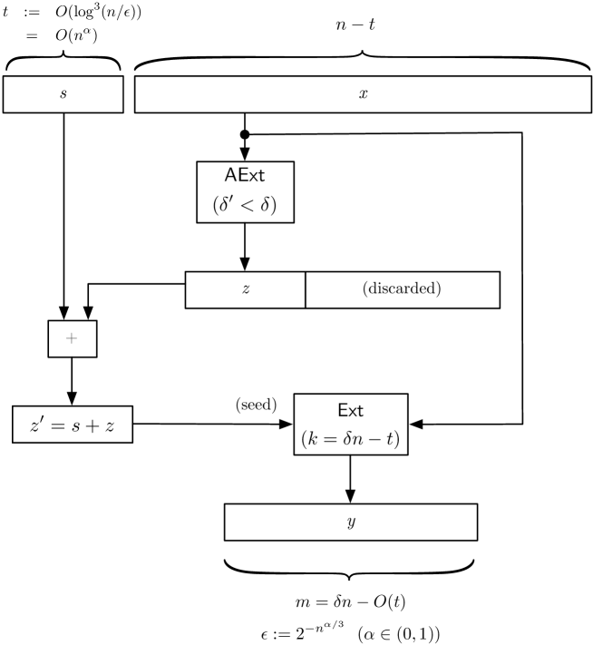
Figure 4: Construction of the invertible affine extractor.

First we show that this is an affine extractor. Suppose that $(S,X)\in\mathds{F}_{2}^{t}\times\mathds{F}_{2}^{n^{\prime}}$ is a random variable sampled from an affine distribution with min-entropy $\delta n$. The variable $S$ can have an affine dependency on $X$. Hence, for every fixed $s\in\mathds{F}_{2}^{t}$, the distribution of $X$ conditioned on the event $S=s$ is affine with min-entropy at least $\delta n-t$, which is at least $\delta^{\prime}n^{\prime}$ for large enough $n$. Hence $\mathsf{AExt}(X)$ will be $2^{-\Omega(n)}$-close to uniform by Theorem 3.9. This implies that $\mathsf{AExt}(X)|_{[t]}+S$ can extract $t$ random bits from the affine source with error $2^{-\Omega(n)}$. Combining this with Theorem 3.21, noticing the fact that the class of affine extractors is closed with respect to linear seeded extractors, we conclude that $D$ is an affine extractor with error at most $\epsilon+2^{-\Omega(n)}\cdot 2^{t+3}=O(2^{-n^{\alpha/3}})$.

Now the inverter works as follows: Given $y\in\mathds{F}_{2}^{m}$, first it picks $Z\in\mathds{F}_{2}^{t}$ uniformly at random. The seeded extractor $\mathsf{Ext}$, given the seed $Z$ is a linear function $\mathsf{Ext}_{Z}\colon\mathds{F}_{2}^{n^{\prime}}\to\mathds{F}_{2}^{m}$. Without loss of generality, assume that this function is surjective. Then the inverter picks $X\in\mathds{F}_{2}^{n^{\prime}}$ uniformly at random from the affine subspace defined by the linear constraint $\mathsf{Ext}_{Z}(X)=y$, and outputs $(Z+\mathsf{AExt}(X)|_{[t]},X)$. It is easy to verify that the output is indeed a valid preimage of $y$. To see the uniformity of the inverter, note that if $y$ is chosen uniformly at random, the distribution of $(Z,X)$ will be uniform on $\mathds{F}_{2}^{n}$. Hence $(Z+\mathsf{AExt}(X)|_{[t]},X)$, which is the output of the inverter, will be uniform. ∎

In the above construction we are using an affine and a linear seeded extractor as black boxes, and hence, they can be replaced by any other extractors as well (the construction will achieve an optimal rate provided that the seeded extractor extracts almost the entire source entropy). In particular, over large fields one can use the affine and seeded extractors given by Gabizon and Raz [ref:affine] that work for sub-constant entropy rates as well.

Moreover, for concreteness we described and instantiated our construction over the binary field. Observe that Shaltiel’s result, for the special case of affine sources, holds regardless of the alphabet size. Moreover, Trevisan’s linear seeded extractor can be naturally extended to handle arbitrary alphabets. Hence, in order to extend our result to non-binary alphabets, it suffices to ensure that a suitable seedless affine extractor that supports the desired alphabet size is available. Bourgain’s original result [ref:Bourgain] is stated and proved for the binary alphabet; however, it seems that this result can be adapted to work for larger fields as well [ref:BourPriv]. Such an extension (along with some improvements and simplifications) is made explicit by Yehudayoff [ref:Yeh09].

An affine extractor is in particular, a symbol-fixing extractor. Hence Theorem 3.24, combined with Lemma 3.15 gives us a wiretap protocol with almost optimal parameters:

Theorem 3.25.

Let $\delta\in[0,1)$ and $\alpha\in(0,1/3)$ be constants. Then for a prime power $q>1$ and every large enough $n$ there is a $(\delta n,O(2^{-n^{\alpha}}),0)_{q}$-resilient wiretap protocol with block length $n$ and rate $1-\delta-o(1)$. ∎

10 Further Applications

In this section we will sketch some important applications of our technique to more general wiretap problems.

10.1 Noisy Channels and Active Intruders

Suppose that Alice wants to transmit a particular sequence to Bob through a noisy channel. She can use various techniques from coding theory to encode her information and protect it against noise. Now what if there is an intruder who can partially observe the transmitted sequence and even manipulate it? Modification of the sequence by the intruder can be regarded in the same way as the channel noise; thus one gets security against active intrusion as a “bonus” by constructing a code that is resilient against noise and passive eavesdropping. There are two natural and modular approaches to construct such a code.

A possible attempt would be to first encode the message using a good error-correcting code and then applying a wiretap encoder to protect the encoded sequence against the wiretapper. However, this will not necessarily keep the information protected against the channel noise, as the combination of the wiretap encoder and decoder does not have to be resistant to noise.

Another attempt is to first use a wiretap encoder and then apply an error-correcting code on the resulting sequence. Here it is not necessarily the case that the information will be kept secure against intrusion anymore, as the wiretapper now gets to observe the bits from the channel-encoded sequence that may reveal information about the original sequence. However, the wiretap protocol given in Theorem 3.25 is constructed from an invertible affine extractor, and guarantees resiliency even if the intruder is allowed to observe arbitrary linear combinations of the transmitted sequence (in this case, the distribution of the encoded sequence subject to the intruder’s observation becomes an affine source and thus, the arguments of the proof of Lemma 3.15 remain valid). In particular, Theorem 3.25 holds even if the intruder’s observation is allowed to be obtained after applying any arbitrary linear mapping on the output of the wiretap encoder. Hence, we can use the wiretap scheme as an outer code and still ensure privacy against an active intruder and reliability in presence of a noisy channel, provided that the error-correcting code being used as the inner code is linear. This immediately gives us the following result:

Theorem 3.26.

Suppose that there is a $q$-ary linear error-correcting code with rate $r$ that is able to correct up to a $\tau$ fraction of errors (via unique or list decoding). Then for every constant $\delta\in[0,1)$ and $\alpha\in(0,1/3)$ and large enough $n$, there is a $(\delta n,O(2^{-n^{\alpha}}),0)_{q}$-resilient wiretap protocol with block length $n$ and rate $r-\delta-o(1)$ that can also correct up to a $\tau$ fraction of errors. ∎

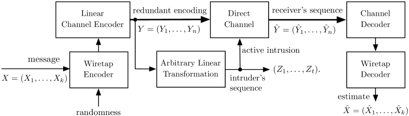
Figure 5: Wiretap scheme composed with channel coding. If the wiretap scheme is constructed by an invertible affine extractor, it can guarantee secrecy even in presence of arbitrary linear manipulation of the information. Active intrusion can be defied using an error-correcting inner code.

The setting discussed above is shown in Figure 5. The same idea can be used to protect fountain codes, e.g., LT- [ref:LT] and Raptor Codes [ref:Raptor], against wiretappers without affecting the error correction capabilities of the code.

Obviously this simple composition idea can be used for any type of channel so long as the inner code is linear, at the cost of reducing the total rate by almost $\delta$. Hence, if the inner code achieves the Shannon capacity of the direct channel (in the absence of the wiretapper), the composed code will achieve the capacity of the wiretapped channel, which is less than the original capacity by $\delta$ [ref:CK78].

10.2 Network Coding

Our wiretap protocol from invertible affine extractors is also applicable in the more general setting of transmission over networks. A communication network can be modeled as a directed graph, in which nodes represent the network devices and information is transmitted along the edges. One particular node is identified as the source and $m$ nodes are identified as receivers. The main problem in network coding is to have the source reliably transmit information to the receivers at the highest possible rate, while allowing the intermediate nodes arbitrarily process the information along the way.

Suppose that, in the graph that defines the topology of the network, the min-cut between the source to each receiver is $n$. It was shown in [ref:NetCod1] that the source can transmit information up to rate $n$ (symbols per transmission) to all receivers (which is optimal), and in [ref:NetCod2, ref:NetCod3] that linear network coding is in fact sufficient to achieve this rate. That is, the transmission at rate $n$ is possible when the intermediate nodes are allowed to forward packets that are (as symbols over a finite field) linear combinations of the packets that they receive (See [ref:NetCodBook] for a comprehensive account of these and other relevant results).

A basic example is shown by the butterfly network in Figure 6. This network consists of a source on the top and two receivers on the bottom, where the min-cut to each receiver is $2$. Without processing the incoming data, as in the left figure, one of the two receivers may receive information at the optimal rate of $2$ symbols per transmission (namely, receiver $1$ in the figure). However, due to the bottleneck existing in the middle (shown by the thick edge $a\to b$), the other receiver will be forced to receive at an inferior rate of $1$ symbol per transmission. However, if linear processing of the information is allowed, node $a$ may combine its incoming information by treating packets as symbols over a finite field and adding them up, as in the right figure. Both receivers may then solve a full-rank system of linear equations to retrieve the original source symbols $x_{1}$ and $x_{2}$, and thereby achieve the optimal min-cut rate.

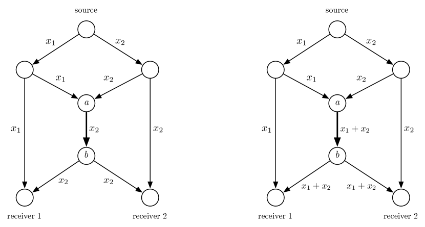
Figure 6: Network coding (right), versus unprocessed forwarding (left).

Designing wiretap protocols for networks is an important question in network coding, which was first posed by Cai and Yeung [ref:NetWT]. In this problem, an intruder can choose a bounded number, say $t$, of the edges and eavesdrop all the packets going through those edges. They designed a network code that could provide the optimal multicast rate of $n-t$ with perfect privacy. However this code requires an alphabet size of order $\binom{|E|}{t}$, where $E$ is the set of edges. Their result was later improved in [ref:FMSS04] who showed that a random linear coding scheme can provide privacy with a much smaller alphabet size if one is willing to achieve a slightly sub-optimal rate. Namely, they obtain rate $n-t(1+\epsilon)$ with an alphabet of size roughly $\mathrm{\Theta}(|E|^{1/\epsilon})$, and show that achieving the exact optimal rate is not possible with small alphabet size.

El Rouayheb and Soljanin [ref:Emina] suggested to use the original code of Ozarow and Wyner [ref:Wyner2] as an outer code at the source and showed that a careful choice of the network code can provide optimal rate with perfect privacy. However, their code eventually needs an alphabet of size at least $\binom{|E|-1}{t-1}+m$. Building upon this work, Silva and Kschischang [ref:RankMetric] constructed an outer code that provides similar results while leaving the underlying network code unchanged. However, their result comes at the cost of increasing the packet size by a multiplicative factor of at least the min-cut bound, $n$ (or in mathematical terms, the original alphabet size $q$ of the network is enlarged to at least $q^{n}$). For practical purposes, this is an acceptable solution provided that an estimate on the min-cut size of the network is available at the wiretap encoder.

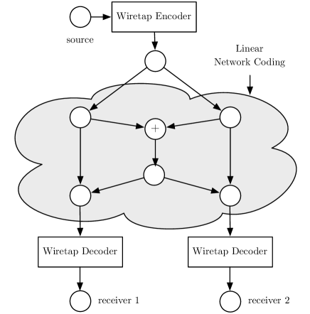
Figure 7: Linear network coding with an outer layer of wiretap encoding added for providing secrecy.

By the discussion presented in Section 10.1, the rate-optimal wiretap protocol given in Theorem 3.25 stays resilient even in presence of any linear post-processing of the encoded information. Thus, using the wiretap encoder given by this result as an outer-code in the source node, one can construct an asymptotically optimal wiretap protocol for networks that is completely unaware of the network and eliminates all the restrictions in the above results. This is schematically shown in Figure 7. Hence, extending our notion of $(t,\epsilon,\gamma)_{q}$-resilient wiretap protocols naturally to communication networks, we obtain the following:

Theorem 3.27.

Let $\delta\in[0,1)$ and $\alpha\in(0,1/3)$ be constants, and consider a network that uses a linear coding scheme over a finite field $\mathds{F}_{q}$ for reliably transmitting information at rate $R$. Suppose that, at each transmission, an intruder can arbitrarily observe up to $\delta R$ intermediate links in the network. Then the source and the receiver nodes can use an outer code of rate $1-\delta-o(1)$ (obtaining a total rate of $R(1-\delta)-o(1)$) which is completely independent of the network, leaves the network code unchanged, and provides almost perfect privacy with error $O(2^{-{R}^{\alpha}})$ and zero leakage over a $q$-ary alphabet. ∎

In addition to the above result that uses the invertible affine extractor of Theorem 3.24, it is possible to use other rate-optimal invertiable affine extractors. In particular, observe that the restricted affine extractor of Theorem 3.11 (and in particular, Corollary 3.12) is a linear function (over the extension field) and is thus, obviously has an efficient $0$-inverter (since inverting the extractor amounts to solving a system of linear equations). By using this extractor (instantiated with Gabidulin’s MRD codes as in Corollary 3.12), we may recover the result of Silva and Kschischang [ref:RankMetric] in our framework. More precisely, we have the following result:

Corollary 3.28.

Let $q$ be any prime power, and consider a network with minimum cut of size $n$ that uses a linear coding scheme over $\mathds{F}_{q}$ for reliably transmitting information at rate $R$. Suppose that, at each transmission, an intruder can arbitrarily observe up to $\delta R$ intermediate links in the network, for some $\delta\in[0,1)$. Then the source and the receiver nodes can use an outer code of rate $1-\delta$ over $\mathds{F}_{q^{n}}$ (obtaining a total rate of $R(1-\delta)$) that provides perfect privacy over a $q^{n}$-ary alphabet. ∎

10.3 Arbitrary Processing

In this section we consider the erasure wiretap problem in its most general setting, which is still of practical importance. Suppose that the information emitted by the source goes through an arbitrary communication medium and is arbitrarily processed on the way to provide protection against noise, to obtain better throughput, or for other reasons. Now consider an intruder who is able to eavesdrop a bounded amount of information at various points of the channel. One can model this scenario in the same way as the original point-to-point wiretap channel problem, with the difference that instead of observing $t$ arbitrarily chosen bits, the intruder now gets to choose an arbitrary Boolean circuit $\mathcal{C}$ with $t$ output bits (which captures the accumulation of all the intermediate processing) and observes the output of the circuit when applied to the transmitted sequence.

Obviously there is no way to guarantee resiliency in this setting, since the intruder can simply choose $\mathcal{C}$ to compute $t$ output bits of the wiretap decoder. However, suppose that in addition there is an auxiliary communication channel between the source and the receiver (that we call the side channel) that is separated from the main channel, and hence, the information passed through the two channel do not blend together by the intermediate processing.

We call this scenario the general wiretap problem, and extend our notion of $(t,\epsilon,\gamma)$-resilient protocol to this problem, with the slight modification that now the output of the encoder (and the input of the decoder) is a pair of strings $(y_{1},y_{2})\in\mathds{F}_{2}^{n}\times\mathds{F}_{2}^{d}$, where $y_{1}$ (resp., $y_{2}$) is sent through the main (resp., side) channel. Now we call $n+d$ the block length and let the intruder choose an arbitrary pair of circuits $(\mathcal{C}_{1},\mathcal{C}_{2})$, one for each channel, that output a total of $t$ bits, and observe $(\mathcal{C}_{1}(y_{1}),\mathcal{C}_{2}(y_{2}))$.

The information-theoretic upper bounds for the achievable rates in the original wiretap problem obviously extend to the general wiretap problem as well. Below we show that for the general problem, secure transmission is possible at asymptotically optimal rates even if the intruder intercepts the entire communication passing through the side channel (as shown in Figure 8).

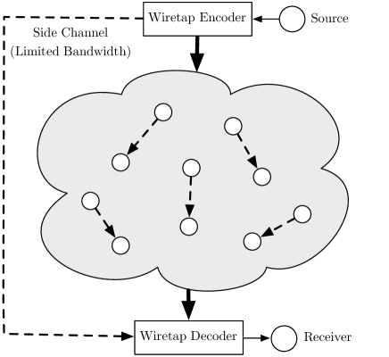
Figure 8: The wiretap channel problem in presence of arbitrary intermediate processing. In this example, data is transmitted over a packet network (shown as a cloud) in which some intermediate links (showed by the dashed arrows) are accessible to an intruder.

Similar as before, our idea is to use invertible extractors to construct general wiretap protocols, but this time we use invertible strong seeded extractors. Strong seeded extractors were used in [ref:CDH] to construct ERFs, and this is exactly what we use as the decoder in our protocol. As the encoder we will use the corresponding inverter, which outputs a pair of strings, one for the extractor’s input which is sent through the main channel and another as the seed which is sent through the side channel. Hence we will obtain the following result:

Theorem 3.29.

Let $\delta\in[0,1)$ be a constant. Then for every $\alpha,\epsilon>0$, there is a $(\delta n,\epsilon,2^{-\alpha n}+\epsilon)$-resilient wiretap protocol for the general wiretap channel problem that sends $n$ bits through the main channel and $d:=O(\log^{3}(n/\epsilon^{2}))$ bits through the side channel and achieves rate $1-\delta-\alpha-O(d/(n+d))$. The protocol is secure even when the entire communication through the side channel is observable by the intruder.

Proof.

We will need the following claim in our proof, which is easy to verify using an averaging argument:

Claim.

Let $f\colon\{0,1\}^{n}\to\{0,1\}^{\delta n}$ be a Boolean function. Then for every $\alpha>0$, and $X\sim\mathcal{U}_{n}$, the probability that $f(X)$ has fewer than $2^{n(1-\delta-\alpha)}$ preimages is at most $2^{-\alpha n}$.

Now, let $\mathsf{Ext}$ be the linear seeded extractor of Theorem 3.22, set up for input length $n$, seed length $d=O(\log^{3}(n/\epsilon^{2}))$, min-entropy $n(1-\delta-\alpha)$, and output length $m=n(1-\delta-\alpha)-O(d)$, and error $\epsilon^{2}$. Then the encoder chooses a seed $Z$ for the extractor uniformly at random and sends it through the side channel.

For the chosen value of $Z$, the extractor is a linear function, and as before, given a message $x\in\{0,1\}^{m}$, the encoder picks a random vector in the affine subspace that is mapped by this linear function to $x$ and sends it through the public channel.

The decoder, in turn, applies the extractor to the seed received from the secure channel and the transmitted string. The resiliency of the protocol can be shown in a similar manner as in Lemma 3.15. Specifically, note that by the above claim, with probability at least $1-2^{-\alpha n}$, the string transmitted through the main channel, conditioned on the observation of the intruder from the main channel, has a distribution $\mathcal{Y}$ with min-entropy at least $n(1-\delta-\alpha)$. Now in addition suppose that the seed $z$ is entirely revealed to the intruder. As the extractor is strong, with probability at least $1-\epsilon$, $z$ is a good seed for $\mathcal{Y}$, meaning that the output of the extractor applied to $\mathcal{Y}$ and seed $z$ is $\epsilon$-close to uniform (by Proposition 2.11), and hence the view of the intruder on the original message remains $\epsilon$-close to uniform. ∎

We observe that it is not possible to guarantee zero leakage for the general wiretap problem above. Specifically, suppose that $(\mathcal{C}_{1},\mathcal{C}_{2})$ are chosen in a way that they have a single preimage for a particular output $(w_{1},w_{2})$. With nonzero probability the observation of the intruder may turn out to be $(w_{1},w_{2})$, in which case the entire message is revealed. Nevertheless, it is possible to guarantee negligible leakage as the above theorem does. Moreover, when the general protocol above is used for the original wiretap II problem (where there is no intermediate processing involved), there is no need for a separate side channel and the entire encoding can be transmitted through a single channel. Contrary to Theorem 3.25 however, the general protocol will not guarantee zero leakage even for this special case.

Appendix 3.A Some Technical Details

This appendix is devoted to some technical details that are omitted in the main text of the chapter.

The following proposition quantifies the Shannon entropy of a distribution that is close to uniform:

Proposition 3.30.

Let $\mathcal{X}$ be a probability distribution on a finite set $S$, $|S|>4$, that is $\epsilon$-close to the uniform distribution on $S$, for some $\epsilon\leq 1/4$. Then $H(\mathcal{X})\geq\log_{2}|S|(1-\epsilon)$

Proof.

Let $n:=|S|$, and let $f(x):=-x\log_{2}x$. The function $f(x)$ is concave, passes through the origin and is strictly increasing in the range $[0,1/\mathrm{e}]$. From the definition, we have $H(\mathcal{X})=\sum_{s\in S}f(\Pr_{\mathcal{X}}(s))$. For each term $s$ in this summation, the probability that $\mathcal{X}$ assigns to $s$ is either at least $1/n$, which makes the corresponding term at least $\log_{2}n/n$ (due to the particular range of $|S|$ and $\epsilon$), or is equal to $1/n-\epsilon_{s}$, for some $\epsilon_{s}>0$, in which case the term corresponding to $s$ is less than $\log_{2}n/n$ by at most $\epsilon_{s}\log_{2}n$ (this follows by observing that the slope of the line connecting the origin to the point $(1/n,f(1/n))$ is $\log_{2}n$). The bound on the statistical distance implies that the differences $\epsilon_{s}$ add up to at most $\epsilon$. Hence, the Shannon entropy of $\mathcal{X}$ can be less than $\log_{2}n$ by at most $\epsilon\log_{2}n$. ∎

Proposition 3.31.

Let $(X,Y)$ be a pair of random variables jointly distributed on a finite set $\Omega\times\Gamma$. Then $\mathbb{E}_{Y}[{\mathsf{dist}}(X|Y,X)]=\mathbb{E}_{X}[{\mathsf{dist}}(Y|X,Y)].$

Proof.

For $x\in\Omega$ and $y\in\Gamma$, we will use shorthands $p_{x},p_{y},p_{xy}$ to denote $\Pr[X=x],\Pr[Y=y],\Pr[X=x,Y=y]$, respectively. Then we have

$$\mathbb{E}_{Y}[{\mathsf{dist}}(X|Y,X)] = \sum_{y\in\Gamma}p_{y}{\mathsf{dist}}(X|(Y=y),X)=\frac{1}{2}\sum_{y\in\Gamma}p_{y}\sum_{x\in\Omega}|p_{xy}/p_{y}-p_{x}|$$

$$= \frac{1}{2}\sum_{y\in\Gamma}\sum_{x\in\Omega}|p_{xy}-p_{x}p_{y}|=\frac{1}{2}\sum_{x\in\Omega}p_{x}\sum_{y\in\Gamma}|p_{xy}/p_{x}-p_{y}|$$

$$= \sum_{x\in\Omega}p_{x}{\mathsf{dist}}(Y|(X=x),Y)=\mathbb{E}_{X}[{\mathsf{dist}}(Y|X,Y)].$$

∎

Proposition 3.32.

Let $\Omega$ be a finite set that is partitioned into subsets $S_{1},\ldots,S_{k}$ and suppose that $\mathcal{X}$ is a distribution on $\Omega$ that is $\gamma$-close to uniform. Denote by $p_{i}$, $i=1,\ldots k$, the probability assigned to the event $S_{i}$ by $\mathcal{X}$. Then

$$\sum_{i\in[k]}p_{i}\cdot{\mathsf{dist}}(\mathcal{X}|S_{i},\mathcal{U}_{S_{i}})\leq 2\gamma.$$

Proof.

Let $N:=|\Omega|$, and define for each $i$, $\gamma_{i}:=\sum_{s\in S_{i}}\left|\Pr_{\mathcal{X}}(s)-\frac{1}{N}\right|,$ so that $\gamma_{1}+\cdots+\gamma_{k}\leq 2\gamma$. Observe that by triangle’s inequality, for every $i$ we must have $|p_{i}-|S_{i}|/N|\leq\gamma_{i}$. To conclude the claim, it is enough to show that for every $i$, we have ${\mathsf{dist}}(\mathcal{X}|S_{i},\mathcal{U}_{S_{i}})\leq\gamma_{i}/p_{i}$. This is shown in the following.

$$p_{i}\cdot{\mathsf{dist}}(\mathcal{X}|S_{i},\mathcal{U}_{S_{i}}) = \frac{p_{i}}{2}\sum_{s\in S_{i}}\left|\frac{\Pr_{\mathcal{X}}(s)}{p_{i}}-\frac{1}{|S_{i}|}\right|$$

$$= \frac{1}{2}\sum_{s\in S_{i}}\left|\Pr_{\mathcal{X}}(s)-\frac{p_{i}}{|S_{i}|}\right|$$

$$= \frac{1}{2}\sum_{s\in S_{i}}\left|\left(\Pr_{\mathcal{X}}(s)-\frac{1}{N}\right)+\frac{1}{|S_{i}|}\left(\frac{|S_{i}|}{N}-p_{i}\right)\right|$$

$$\leq \frac{1}{2}\sum_{s\in S_{i}}\left|\Pr_{\mathcal{X}}(s)-\frac{1}{N}\right|+\frac{1}{2|S_{i}|}\sum_{s\in S_{i}}\left|\frac{|S_{i}|}{N}-p_{i}\right|$$

$$\leq \frac{\gamma_{i}}{2}+\frac{1}{2|S_{i}|}\cdot|S_{i}|\gamma_{i}=\gamma_{i}.$$

∎

The following proposition shows that any function maps close distributions to close distributions:

Proposition 3.33.

Let $\Omega$ and $\Gamma$ be finite sets and $f$ be a function from $\Omega$ to $\Gamma$. Suppose that $\mathcal{X}$ and $\mathcal{Y}$ are probability distributions on $\Omega$ and $\Gamma$, respectively, and let $\mathcal{X^{\prime}}$ be a probability distribution on $\Omega$ which is $\delta$-close to $\mathcal{X}$. Then if $f(\mathcal{X})\sim_{\epsilon}\mathcal{Y}$, then $f(\mathcal{X^{\prime}})\sim_{\epsilon+\delta}\mathcal{Y}$.

Proof.

Let $X$, $X^{\prime}$ and $Y$ be random variables distributed according to $\mathcal{X}$, $\mathcal{X^{\prime}}$, and $\mathcal{Y}$, respectively. We want to upperbound

$$\left|\Pr[f(X^{\prime})\in T]-\Pr[Y\in T]\right|$$

for every $T\subseteq\Gamma$. By the triangle inequality, this is no more than

$$\left|\Pr[f(X^{\prime})\in T]-\Pr[f(X)\in T]\right|+\left|\Pr[f(X)\in T]-\Pr[Y\in T]\right|.$$

Here the summand on the right hand side is upperbounded by the distance of $f(\mathcal{X})$ and $\mathcal{Y}$, that is assumed to be at most $\epsilon$. Let $T^{\prime}:=\{x\in\Omega\mid f(x)\in T\}$. Then the summand on the left can be written as

$$\left|\Pr[X^{\prime}\in T^{\prime}]-\Pr[X\in T^{\prime}]\right|$$

which is at most $\delta$ by the assumption that $\mathcal{X}\sim_{\delta}\mathcal{X^{\prime}}$. ∎

Omitted Details of the Proof of Corollary 3.19

Here we prove Corollary 3.19 for the case $c>1$. The construction is similar to the case $c=1$, and in particular the choice of $m$ and $k$ will remain the same. However, a subtle complication is that the expander family may not have a graph with $d^{m}$ vertices and we need to adapt the extractor of Theorem 3.18 to support our parameters, still with exponentially small error. To do so, we pick a graph $G$ in the family with $N$ vertices, such that

$$c^{\eta m}d^{m}\leq N\leq c^{\eta m+1}d^{m},$$

for a small absolute constant $\eta>0$ that we are free to choose. The assumption on the expander family guarantees that such a graph exists. Let $m^{\prime}$ be the smallest integer such that $d^{m^{\prime}}\geq c^{\eta m}N$. Index the vertices of $G$ by integers in $[N]$. Note that $m^{\prime}$ will be larger than $m$ by a constant multiplicative factor that approaches $1$ as $\eta\to 0$.

For positive integers $q$ and $p\leq q$, define the function $\mathsf{Mod}_{q,p}\colon[q]\to[p]$ by

$$\mathsf{Mod}_{q,p}(x):=1+(x\ \mathrm{mod}\ p).$$

The extractor $\mathsf{SFExt}$ interprets the first $m^{\prime}$ symbols of the input as an integer $u$, $0\leq u<d^{m^{\prime}}$ and performs a walk on $G$ starting from the vertex $\mathsf{Mod}_{d^{m^{\prime}},N}(u+1)$, the walk being defined by the remaining input symbols. If the walk reaches a vertex $v$ at the end, the extractor outputs $\mathsf{Mod}_{N,d^{m}}(v)-1$, encoded as a $d$-ary string of length $m$. A similar argument as in Theorem 3.18 can show that with our choice of the parameters, the extractor has an exponentially small error, where the error exponent is now inferior to that of Theorem 3.18 by $O(m)$, but the constant behind $O(\cdot)$ can be made arbitrarily small by choosing a sufficiently small $\eta$.

The real difficulty lies with the inverter because $\mathsf{Mod}$ is not a balanced function (that is, all images do not have the same number of preimages), thus we will not be able to obtain a perfect inverter. Nevertheless, it is possible to construct an inverter with a close-to-uniform output in $\ell_{\infty}$ norm. This turns out to be as good as having a perfect inverter, and thanks to the following lemma, we will still be able to use it to construct a wiretap protocol with zero leakage:

Lemma 3.34.

Suppose that $f\colon[d]^{n}\rightarrow[d]^{m}$ is a $(k,2^{-\Omega(m)})_{d}$ symbol-fixing extractor and that $\mathcal{X}$ is a distribution on $[d]^{n}$ such that $\|\mathcal{X}-\mathcal{U}_{[d]^{n}}\|_{\infty}\leq 2^{-\Omega(m)}/d^{n}$. Denote by $\mathcal{X}^{\prime}$ the distribution $\mathcal{X}$ conditioned on any fixing of at most $n-k$ coordinates. Then $f(\mathcal{X}^{\prime})\sim_{2^{-\Omega(m)}}\mathcal{U}_{[d]^{m}}$.

Proof.

By Proposition 3.33, it suffices to show that $\mathcal{X}^{\prime}$ is $2^{-\Omega(m)}$-close to an $(n,k)_{d}$ symbol-fixing source. Let $S\subseteq[d]^{m}$ denote the support of $\mathcal{X}^{\prime}$, and let $\epsilon/d^{n}$ be the $\ell_{\infty}$ distance between $\mathcal{X}$ and $\mathcal{U}_{[d]^{n}}$, so that by our assumption, $\epsilon=2^{-\Omega(m)}$. By the bound on the $\ell_{\infty}$ distance, we know that $\Pr_{\mathcal{X}}(S)$ is between $\frac{|S|}{d^{n}}(1-\epsilon)$ and $\frac{|S|}{d^{n}}(1+\epsilon)$. Hence for any $x\in S$, $\Pr_{\mathcal{X}^{\prime}}(x)$, which is $\Pr_{\mathcal{X}}(x)/\Pr_{\mathcal{X}}(S)$, is between $\frac{1}{|S|}\cdot\frac{1-\epsilon}{1+\epsilon}$ and $\frac{1}{|S|}\cdot\frac{1+\epsilon}{1-\epsilon}$. This differs from $1/|S|$ by at most $O(\epsilon)/|S|$. Hence, $\mathcal{X}^{\prime}$ is $2^{-\Omega(m)}$-close to $\mathcal{U}_{S}$. ∎

In order to invert our new construction, we will need to construct an inverter $\mathsf{Inv}_{q,p}$ for the function $\mathsf{Mod}_{q,p}$. For that, given $x\in[p]$ we will just sample uniformly in its preimages. This is where the non-balancedness of $\mathsf{Mod}$ causes problems, since if $p$ does not divide $q$ the distribution $\mathsf{Inv}_{q,p}(\mathcal{U}_{[p]})$ is not uniform on $[q]$.

Lemma 3.35.

Suppose that $q>p$. Given a distribution $\mathcal{X}$ on $[p]$ such that $\|\mathcal{X}-\mathcal{U}_{[p]}\|_{\infty}\leq\frac{\epsilon}{p}$, we have $\|\mathsf{Inv}_{q,p}(\mathcal{X})-\mathcal{U}_{[q]}\|_{\infty}\leq\frac{1}{q}\cdot\frac{p+\epsilon q}{q-p}$.

Proof.

Let $X\sim\mathcal{X}$ and $Y\sim\mathsf{Inv}_{q,p}(\mathcal{X})$. Since we invert the modulo function by taking for a given output a random preimage uniformly, $\Pr[Y=y]$ is equal to $\Pr[X=\mathsf{Mod}_{q,p}(y)]$ divided by the number of $y$ with the same value for $\mathsf{Mod}_{q,p}(y)$. The latter number is either $\lfloor q/p\rfloor$ or $\lceil q/p\rceil$, so

$$\frac{1-\epsilon}{p\lceil q/p\rceil}\leq\Pr(Y=y)\leq\frac{1+\epsilon}{p\lfloor q/p\rfloor}$$

Bounding the floor and ceiling functions by $q/p\pm 1$, we obtain

$$\frac{1-\epsilon}{q+p}\leq\Pr(Y=y)\leq\frac{1+\epsilon}{q-p}$$

That is

$$\frac{-p-\epsilon q}{q(q+p)}\leq\Pr(Y=y)-\frac{1}{q}\leq\frac{p+\epsilon q}{q(q-p)}\ ,$$

which concludes the proof since this is true for all $y$. ∎

Now we describe the inverter $\mathsf{Inv}(x)$ for the extractor, again abusing the notation. First the inverter calls $\mathsf{Inv}_{N,d^{m}}(x)$ to obtain $x_{1}\in[N]$. Then it performs a random walk on the graph, starting from $x_{1}$, to reach a vertex $x_{2}$ at the end which is inverted to obtain $x_{3}=\mathsf{Inv}_{d^{m^{\prime}},N}(x_{2})$ as a $d$-ary string of length $m^{\prime}$. Finally, the inverter outputs $y=(x_{3},w)$, where $w$ corresponds the inverse of the random walk of length $n-m^{\prime}$. It is obvious that this procedure yields a valid preimage of $x$.

Using the previous lemma, if $x$ is chosen uniformly, $x_{1}$ will be at $\ell_{\infty}$-distance

$$\epsilon_{1}:=\frac{1}{N}\cdot\frac{d^{m}}{N-d^{m}}=\frac{1}{N}O(c^{-\eta m}).$$

For a given walk, the distribution of $x_{2}$ will just be a permutation of the distribution of $x_{1}$ and applying the lemma again, we see that the $\ell_{\infty}$-distance of $x_{3}$ from the uniform distribution is

$$\epsilon_{2}:=\frac{1}{d^{m^{\prime}}}\cdot\frac{N+\epsilon_{1}d^{m^{\prime}}}{d^{m^{\prime}}-N}=\frac{1}{d^{m^{\prime}}}O(c^{-\eta m}).$$

This is true for all the $d^{n-m^{\prime}}$ possible walks so the $\ell_{\infty}$-distance of the distribution of $y$ from uniform is bounded by $\frac{1}{d^{n}}O(c^{-\eta m})$. Applying Lemma 3.34 in an argument similar to Lemma 3.15 concludes the proof.

   

Domenico Scarlatti (1685–1757): Keyboard Sonata
in B minor K. 87 (L. 33).

Chapter 4 Group Testing

70

The history of group testing is believed to date back to the second World War. During the war, millions of blood samples taken from draftees had to be subjected to a certain test, and be analyzed in order to identify a few thousand cases of syphilis. The tests were identical for all the samples. Here the idea of group testing came to a statistician called Robert Dorfman (and perhaps, a few other researchers working together with him, among them David Rosenblatt). He made a very intuitive observation, that, the samples are constantly subjected to the same test, which is extremely sensitive and remains reliable even if the sample is diluted. Therefore, it makes sense to, instead of analyzing each sample individually, pool every few samples in a group, and apply the test on the mixture of the samples. If the test outcome is negative, we will be sure that none of the samples participating in the pool are positive. On the other hand, if the outcome is positive, we know that one or more of the samples are positive, and will have to proceed with more refined, or individual, tests in order to identify the individual positives within the group.

Since the number of positives in the entire population was suspected to be in order of a few thousands—a small fraction of the population—Dorfman’s idea would save a great deal of time and resources. Whether or not the idea had been eventually implemented at the time, Dorfman went on to publish a paper on the topic [ref:Dor43], which triggered an extensive line of research in combinatorics known today as combinatorial group testing.

The main challenge in group testing is to design the pools in such a way to minimize the number of tests required in order to identify the exact set of positives. Larger groups would save a lot of tests if their outcome is negative, and are rather wasteful otherwise (since in the latter case they convey a relatively small amount of information).

Of course the applications of group testing are not limited to blood sampling. To mention another early example, consider a production line of electric items such as light bulbs (or resistors, capacitors, etc). As a part of the quality assurance, defective items have to be identified and discarded. Group testing can be used to aid this process. Suppose that a group of light bulbs are connected in series, and an electric current is passed through the circuit. If all the bulbs are illuminated, we can be sure than none is defective, and otherwise, we know that at least one is defective.

Since its emergence decades ago, group testing has found a large number of surprising applications that are too numerous to be extensively treated here. We particularly refer to applications in molecular biology and DNA library screening (cf. [ref:BKBB95, ref:KKM97, ref:Mac99, ref:ND00, ref:STR03, ref:WHL06, ref:WLHD08] and the references therein), multiaccess communication [ref:Wol85], data compression [ref:HL00], pattern matching [ref:CEPR07], streaming algorithms [ref:CM05], software testing [ref:BG02], compressed sensing [ref:CM06], and secure key distribution [ref:CDH07], among others. Moreover, entire books are specifically targeted to combinatorial group testing [ref:groupTesting, ref:DH06].

In formal terms, the classical group testing problem can be described as follows. Suppose that we wish to “learn” a Boolean vector of length $n$, namely $x=(x_{1},\ldots,x_{n})\in\{0,1\}^{n}$ using as few questions as possible. Each question can ask for a single bit $x_{i}$, or more generally, specify a group of coordinates $\mathcal{I}\subseteq[n]$ ($\mathcal{I}\neq\emptyset$) and ask for the bit-wise “or” of the entries at the specified coordinates; i.e., $\bigvee_{i\in\mathcal{I}}x_{i}$. We will refer to this type of questions as disjunctive queries. Obviously, in order to be able to uniquely identify $x$, there is in general no better way than asking for individual bits $x_{1},\ldots,x_{n}$ (and thus, $n$ questions), since the number of Boolean vectors of length $n$ is $2^{n}$ and thus, information theoretically, $n$ bits of information is required to describe an arbitrary $n$-bit vector. Therefore, without imposing further restrictions on the possible realizations of the unknown vector, the problem becomes trivial.

Motivated by the blood sampling application that we just described, natural restriction that is always assumed in group testing on the unknown vector $x$ is that it is sparse. Namely, for an integer parameter $d>0$, we will assume that the number of nonzero entries of $x$ is at most $d$. We will refer to such a vector as $d$-sparse. The number of $d$-sparse Boolean vectors is

$$\sum_{i=0}^{n}\binom{n}{i}=2^{\Theta(d\log(n/d))},$$

and therefore, in principle, any $d$-sparse Boolean vector can be described using only $O(d\log(n/d))$ bits of information, a number that can be substantially smaller than $n$ if $d\ll n$. The precise interpretation of the assumption “$d\ll n$” varies from a setting to another. For a substantial part of this chapter, one can think of $d=O(\sqrt{n})$. The important question in group testing that we will address in this chapter is that, whether the information-theoretic limit $\Omega(d\log(n/d))$ on the number of questions can be achieved using disjunctive queries as well.

Notation for this chapter: In this chapter we will be constantly working with Boolean vectors and their support. The support of a vector $x=(x_{1},\ldots,x_{n})\in\{0,1\}^{n}$, denoted by $\mathsf{supp}(x)$, is a subset of $[n]$ such that $i\in\mathsf{supp}(x)$ if and only if $x_{i}=1$. Thus the Hamming weight of $x$, that we will denote by $\mathsf{wgt}(x)$ can be defined as $\mathsf{wgt}(x)=|\mathsf{supp}(x)|$, and a $d$-sparse vector has the property that $\mathsf{wgt}(x)\leq d$.