Nonadditive hard-sphere fluid mixtures: A simple analytical theory

Abstract

We construct a non-perturbative fully analytical approximation for the thermodynamics and the structure of non-additive hard-sphere fluid mixtures. The method essentially lies in a heuristic extension of the Percus–Yevick solution for additive hard spheres. Extensive comparison with Monte Carlo simulation data shows a generally good agreement, especially in the case of like-like radial distribution functions.

I Introduction

The van der Waals ideas Hansen and McDonald (2006) show that the most important feature of the pair potential between atoms or molecules is the harsh repulsion that appears at short range and has its origin in the overlap of the outer electron shells. These ideas form the basis of the very successful perturbation theories of the liquid state. This, along with fruitful applications to soft matter Likos (2001), explains the continued interest in hard-sphere reference systems Mulero (2008).

The simplest model for a fluid mixture is a system of additive hard spheres (AHSs) for which the like-unlike collision diameter ($\sigma_{ij}$) between a particle of species $i$ and one of species $j$ is equal to the arithmetic mean $\sigma^{\text{add}}_{ij}\equiv\frac{1}{2}(\sigma_{ii}+\sigma_{jj})$. A more general model consists of nonadditive hard spheres (NAHSs), where the like-unlike collision diameter differs from $\sigma^{\text{add}}_{ij}$ by a quantity $\Delta_{ij}=(\sigma_{ij}-\sigma^{\text{add}}_{ij})/\sigma^{\text{add}}_{ij}$ called the nonadditivity parameter. As mentioned in the paper by Ballone et al. Ballone et al. (1986), where the relevant references may be found, experimental work on alloys, aqueous electrolyte solutions, and molten salts suggests that homocoordination and heterocoordination Gazzillo et al. (1989, 1990) may be interpreted in terms of excluded volume effects due to nonadditivity (positive and negative, respectively) of the repulsive part of the intermolecular potential. NAHS systems are also useful models to describe real physical systems as rare gas mixtures Shouten (1989) and colloids Gast et al. (1983); Lekkerkerker et al. (1992); Dijkstra et al. (1999); Meijer and Frenkel (1994). For a short review of the literature on NAHSs up to 2005 the reader is referred to Ref. Santos et al. (2005).

The well-known Percus–Yevick (PY) integral-equation theory Hansen and McDonald (2006) is exactly solvable for a mixture of three-dimensional (3D) AHS mixtures Lebowitz (1964); Yuste et al. (1998). The solution has been recently extended to any odd dimensionality Rohrmann and Santos (2011). On the other hand, any amount of nonadditivity ($\Delta_{ij}\neq 0$) suffices to destroy the analytical character of the solution and so one needs to resort to numerical methods to solve the PY or other integral equations Ballone et al. (1986).

The aim of the present paper is to propose a non-perturbative and fully analytical approach for 3D NAHS fluid mixtures, which can be seen as a naïve heuristic extension of the PY solution for AHS mixtures. In doing this, we are guided by the exact solution of the one-dimensional (1D) NAHS model Salsburg et al. (1953); Lebowitz and Zomick (1971); Heying and Corti (2004); Santos (2007) and some physical constraints are imposed: the radial distribution function (RDF) $g_{ij}(r)$ must be zero within the diameter $\sigma_{ij}$, the isothermal compressibility must be finite, and the zero density limit of the RDF must be satisfied. We find that this strategy gives very good results both for the thermodynamics and the structure, provided that some geometrical constraints on the diameters and the nonadditivity parameter are satisfied. This makes our approach particularly appealing as a reference approximation for integral equation theories and perturbation theories of fluids.

The paper is organized as follows: in Sec. II we describe the NAHS model outlining the physical constraints that we want to embody in our approach. The latter is constructed by a three-stage procedure (approximations RFA, $\text{RFA}_{+}$, and $\text{RFA}_{+}^{(m)}$) in Sec. III. In Sec. IV we present the results for the equation of state from our approximation, comparing them with available Monte Carlo (MC) simulations. The results for the structural properties are presented in Sec. V, where we compare with our own MC simulations. Finally, Sec. VI is devoted to some concluding remarks.

II The NAHS model

An $n$-component mixture of NAHSs in the $d$-dimensional Euclidean space is a fluid of $N_{i}$ particles of species $i$ (with $i=1,2,\ldots,n$), such that there are a total number of particles $N=\sum_{i=1}^{n}N_{i}$ in a volume $V$, and the pair potential between a particle of species $i$ and a particle of species $j$ separated by a distance $r$ is given by

$$U_{ij}(r)=\left\{\begin{array}[]{ll}\infty,&r<\sigma_{ij},\\ 0,&r>\sigma_{ij},\end{array}\right.$$ (1)

where $\sigma_{ii}=\sigma_{i}$ and $\sigma_{ij}=\frac{1}{2}(\sigma_{i}+\sigma_{j})(1+\Delta_{ij})$, so that $\Delta_{ii}=0$ and $\Delta_{ij}=\Delta_{ji}>-1$. When $\Delta_{ij}=0$ for all pairs $(i,j)$ we recover the AHS system. In a binary mixture ($n=2$), $\Delta_{12}=\Delta_{21}=\Delta$ is the only nonadditivity parameter. If $\Delta=-1$ one recovers the case of two independent one-component hard-sphere (HS) systems. In the other extreme case $\sigma_{1}=\sigma_{2}=0$ with $\sigma_{12}$ finite (so that $\Delta\to\infty$) one obtains the well known Widom–Rowlinson (WR) model Widom and Rowlinson (1970); Ruelle (1971). Another interesting case is the Asakura–Oosawa model Asakura and Oosawa (1954, 1958) (where $\sigma_{2}=0$ and $\Delta>0$), often used to discuss polymer colloid mixtures and where the notion of a depletion potential was introduced. The NAHS system undergoes a demixing phase transition for positive nonadditivity Rovere and Pastore (1994); Jagannathan and Yethiraj (2003); Góźdź (2003); Buhot (2005); Lomba et al. (1996). A demixing transition might also be possible, even for negative nonadditivity Santos and López de Haro (2005); Sillrén and Hansen (2010), provided the asymmetry ratio $\sigma_{1}/\sigma_{2}$ is sufficiently far from unity. In the present paper we will only consider the NAHS system in its single fluid phase.

Let the number density of the mixture be $\rho=N/V$ and the mole fraction of species $i$ be $x_{i}=\rho_{i}/\rho$, where $\rho_{i}=N_{i}/V$ is the number density of species $i$. From these quantities one can define the (nominal) packing fraction $\eta=v_{d}\rho M_{d}$, where $v_{d}=(\pi/4)^{d/2}\Gamma(1+d/2)$ is the volume of a $d$-dimensional sphere of unit diameter and

$$M_{k}\equiv\langle\sigma^{k}\rangle=\sum_{i=1}^{n}x_{i}\sigma_{i}^{k}$$ (2)

denotes the $k$th moment of the diameter distribution.

The NAHS model, in the thermodynamic limit $N\to\infty$ with $\rho\equiv N/V$ constant, admits an analytical exact solution for the structure and the thermodynamics in $d=1$ Salsburg et al. (1953); Lebowitz and Zomick (1971); Heying and Corti (2004); Santos (2007). Moreover, the AHS model in odd dimensions is analytically solvable in the PY approximation Lebowitz (1964); Yuste et al. (1998); Rohrmann and Santos (2011), the result reducing to the exact solution of the problem for $d=1$ but not for $d\geq 3$.

II.1 Basic physical constraints on the structure

The RDF $g_{ij}(r)$ must comply with three basic conditions:

• $g_{ij}(r)$ must vanish for $r<\sigma_{ij}$. More specifically, for distances near $\sigma_{ij}$,

  $$g_{ij}(r)=\Theta(r-\sigma_{ij})\left[g_{ij}(\sigma_{ij}^{+})+g_{ij}^{\prime}(\sigma_{ij}^{+})(r-\sigma_{ij})+\cdots\right],$$ (3)

  where $\Theta(x)$ is the Heaviside step function.

• In the fluid phase the isothermal compressibility $\chi$ must be finite. This implies (see below) that the Fourier transform $\widetilde{h}_{ij}(q)$ of the total correlation function $h_{ij}(r)\equiv g_{ij}(r)-1$ has to remain finite at $q=0$ or, equivalently,

  $$\int_{0}^{\infty}dr\,r^{\alpha}h_{ij}(r)=\mbox{finite for $0\leq\alpha\leq d-1$}.$$ (4)

• In the low density limit, the RDF is

  $$\lim_{\rho\to 0}g_{ij}(r)=e^{-U_{ij}(r)/k_{B}T}=\Theta(r-\sigma_{ij}),$$ (5)

  $k_{B}$ and $T$ being the Boltzmann constant and the absolute temperature, respectively.

As a complement to Eq. (5), we give below the exact expression of $g_{ij}(r)$ to first order in density Yuste et al. (2008):

$$g_{ij}(r) = \Theta(r-\sigma_{ij})\Big{\{}1+\frac{\pi\rho}{12r}\sum_{k=1}^{n}x_{k}\Theta(\sigma_{ik}+\sigma_{kj}-r)$$ (6)

$$\times(r-\sigma_{ik}-\sigma_{kj})^{2}\left[r^{2}+2(\sigma_{ik}+\sigma_{kj})r\right.$$

$$\left.-3(\sigma_{ik}-\sigma_{kj})^{2}\right]+\mathcal{O}(\rho^{2})\Big{\}}.$$

II.2 The two routes to thermodynamics

For an athermal fluid like NAHSs there are two main routes that lead from the knowledge of the structure to the equation of state (EOS) Hansen and McDonald (2006). These may give different results for an approximate RDF.

The virial route to the EOS of the NAHS mixture requires the knowledge of the contact values $g_{ij}(\sigma_{ij}^{+})$ of the RDF,

$$Z^{v}(\eta)=1+\frac{2^{d-1}}{M_{d}}\eta\sum_{i,j=1}^{n}x_{i}x_{j}\sigma_{ij}^{d}g_{ij}(\sigma_{ij}^{+}),$$ (7)

where $Z=p/\rho k_{B}T$ is the compressibility factor of the mixture, $p$ being the pressure.

The isothermal compressibility $\chi$, in a mixture, is in general given by

$$\chi^{-1} = \frac{1}{k_{B}T}\left(\frac{\partial p}{\partial\rho}\right)_{T,\{x_{j}\}}=\frac{1}{k_{B}T}\sum_{i=1}^{n}x_{i}\left(\frac{\partial p}{\partial\rho_{i}}\right)_{T,\{x_{j}\}}$$ (8)

$$= 1-\rho\sum_{i,j=1}^{n}x_{i}x_{j}\widetilde{c}_{ij}(0),$$

where $\widetilde{c}_{ij}(q)$ is the Fourier transform of the direct correlation function $c_{ij}(r)$, which is defined by the Ornstein–Zernike (OZ) equation

$$\widetilde{h}_{ij}(q)=\widetilde{c}_{ij}(q)+\sum_{k=1}^{n}\rho_{k}\widetilde{h}_{ik}(q)\widetilde{c}_{kj}(q).$$ (9)

Introducing the quantities $\widehat{h}_{ij}(q)\equiv\sqrt{\rho_{i}\rho_{j}}\widetilde{h}_{ij}(q)$ and $\widehat{c}_{ij}(q)\equiv\sqrt{\rho_{i}\rho_{j}}\widetilde{c}_{ij}(q)$, the OZ relation becomes, in matrix notation,

$$\widehat{\mathsf{c}}(q)=\widehat{\mathsf{h}}(q)\cdot\left[\mathsf{I}+\widehat{\mathsf{h}}(q)\right]^{-1},$$ (10)

where $\mathsf{I}$ is the $n\times n$ identity matrix. Thus Eq. (8) can be rewritten as

$$\chi^{-1} = \sum_{i,j=1}^{n}\sqrt{x_{i}x_{j}}\left[\delta_{ij}-\widehat{c}_{ij}(0)\right]$$ (11)

$$= \sum_{i,j=1}^{n}\sqrt{x_{i}x_{j}}\left[\mathsf{I}+\widehat{\mathsf{h}}(0)\right]^{-1}_{ij}.$$

In Eq. (11), and henceforth, we use the notation $A_{ij}^{-1}$ to denote the $ij$ element of the inverse $\mathsf{A}^{-1}$ of a given square matrix $\mathsf{A}$.

In the particular case of binary mixtures ($n=2$), Eq. (11) yields

$$\chi=\frac{[1+\rho x_{1}\widehat{h}_{11}(0)][1+\rho x_{2}\widehat{h}_{22}(0)]-\rho^{2}x_{1}x_{2}\widehat{h}_{12}^{2}(0)}{1+\rho x_{1}x_{2}[\widehat{h}_{11}(0)+\widehat{h}_{22}(0)-2\widehat{h}_{12}(0)]}.$$ (12)

The compressibility route to the EOS can be obtained from

$$Z^{c}(\eta)=\int_{0}^{1}{dx}\,{\chi^{-1}(\eta x)}.$$ (13)

II.3 The one-dimensional system

The exact solution for nonadditive hard rods ($d=1$) is known Lebowitz et al. (1962); Santos (2007); Ben-Naim and Santos (2009). First, let us introduce the Laplace transform

$$G_{ij}(s)\equiv\int_{0}^{\infty}dr\,e^{-sr}g_{ij}(r).$$ (14)

In terms of this quantity the exact solution has the form

$$G_{ij}(s)=\frac{1}{\sqrt{x_{i}x_{j}}}\sum_{k=1}^{n}{P}_{ik}(s)Q_{kj}(s),$$ (15)

where

$${P}_{ij}(s)\equiv\sqrt{x_{i}x_{j}}K_{ij}\frac{e^{-\sigma_{ij}(s+\xi)}}{s+\xi}$$ (16)

is proportional to the Laplace transform of the nearest-neighbor probability distribution and

$$\mathsf{Q}(s)\equiv\left[\mathsf{I}-\rho{\mathsf{P}}(s)\right]^{-1}.$$ (17)

In Eqs. (15) and (16), $\xi\equiv p/k_{B}T=\rho Z$, while $K_{ij}=K_{ji}$ are state-dependent parameters that are determined as functions of $\xi$ from the condition (4), which implies $\lim_{s\to 0}sG_{ij}(s)=1$, as well as requiring the ratio $K_{ij}/K_{ik}$ to be independent of $i$ Santos (2007). Those conditions also provide the exact EOS in implicit form, i.e., $\rho$ as a function of $\xi$.

Of course, the above results also hold for additive hard rods. In that case, the additive property $\sigma_{ij}=\sigma^{\text{add}}_{ij}\equiv\frac{1}{2}(\sigma_{i}+\sigma_{j})$ allows us to rewrite the solution in other equivalent ways. To that end, let us define

$$L_{ij}=K_{ij}e^{-\xi\sigma^{\text{add}}_{ij}},$$ (18)

so that

$${P}_{ij}(s)=\sqrt{x_{i}x_{j}}L_{ij}\frac{e^{-\sigma^{\text{add}}_{ij}s}}{s+\xi},$$ (19)

$$Q^{-1}_{ij}(s)=e^{a_{ij}s}\sqrt{\frac{x_{j}}{x_{i}}}\frac{s}{s+\xi}C_{ij}(s),$$ (20)

where

$$a_{ij}\equiv\frac{1}{2}(\sigma_{i}-\sigma_{j})$$ (21)

and

$$C_{ij}(s)\equiv\left(1+\frac{\xi}{s}\right)\delta_{ij}-\frac{\rho x_{i}}{s}L_{ij}e^{-\sigma_{i}s}.$$ (22)

Here we have made use of the property

$$\sigma_{i}=\sigma^{\text{add}}_{ij}+a_{ij}.$$ (23)

It is easy to prove that

$$Q_{ij}(s)=e^{a_{ij}s}\sqrt{\frac{x_{j}}{x_{i}}}\frac{s+\xi}{s}C^{-1}_{ij}(s),$$ (24)

thanks to the property $a_{ik}+a_{kj}=a_{ij}$. Consequently, in the additive case, Eq. (15) becomes

$$G_{ij}^{\text{add}}(s)=\frac{e^{-\sigma^{\text{add}}_{ij}s}}{s}\sum_{k=1}^{n}L_{ik}C^{-1}_{kj}(s),$$ (25)

where use has been made of the additivity property

$$\sigma^{\text{add}}_{ik}-a_{kj}=\sigma^{\text{add}}_{ij}.$$ (26)

The additive solution turns out to be

$$L_{ij}=\frac{\xi}{\rho}=\frac{1}{1-\rho M_{1}}.$$ (27)

The fact that $L_{ij}=\text{const}$ allows one to rewrite Eq. (25) in yet another equivalent form,

$$G_{ij}^{\text{add}}(s)=\frac{e^{-\sigma^{\text{add}}_{ij}s}}{s}\sum_{k=1}^{n}L_{ik}B^{-1}_{kj}(s),$$ (28)

where

$$B_{ij}(s) \equiv \delta_{ij}-\frac{\rho x_{i}}{s}L_{ij}\varphi_{0}(\sigma_{i}s)$$ (29)

$$= C_{ij}(s)+\frac{\xi}{s}\left(x_{i}-\delta_{ij}\right).$$

In the first equality,

$$\varphi_{0}(x)\equiv e^{-x}-1.$$ (30)

While $\lim_{s\to 0}sC_{ij}(s)=\xi\left(\delta_{ij}-x_{i}\right)\neq 0$, but $\det[s\mathsf{C}(s)]=\mathcal{O}(s)$, in the case of the matrix $\mathsf{B}(s)$ one has $\lim_{s\to 0}sB_{ij}(s)=0$. On the other hand, in both cases, $\lim_{s\to\infty}C_{ij}(s)=\lim_{s\to\infty}B_{ij}(s)=\delta_{ij}$, so that $\lim_{s\to\infty}se^{\sigma^{\text{add}}_{ij}}G_{ij}(s)=L_{ij}=\xi/\rho$.

It turns out that Eqs. (25), (27), and (28) are also obtained from the PY solution for additive hard rods. Thus, the PY equation yields the exact solution in the additive case, but not in the nonadditive one.

It is important to bear in mind that, if one inverts the steps, it is possible to formally get Eq. (15) from Eq. (25). In other words, starting from the form (25) of the PY solution for the 1D AHS system, allowing $L_{ij}$ and $\xi$ to be free, and carrying out some formal manipulations, one arrives at an equivalent form, Eq. (15), that, if heuristically extended to the NAHS case ($\sigma_{ij}\neq\sigma^{\text{add}}_{ij}$), coincides with the exact solution to the problem. However, it is not possible to recover (15) starting from the form (28) since the property $L_{ij}=\text{const}$, only valid in the additive case, cannot be reversed.

II.4 PY solution for three-dimensional AHSs

In this subsection we recall the PY solution for AHSs in three dimensions ($d=3$) Lebowitz (1964); Yuste et al. (1998).

First, one introduces the Laplace transform of $rg_{ij}(r)$,

$$G_{ij}(s)\equiv\int_{0}^{\infty}dr\,e^{-sr}rg_{ij}(r).$$ (31)

From Eq. (3) it follows that

$$se^{\sigma_{ij}s}G_{ij}(s) = \sigma_{ij}g_{ij}(\sigma_{ij}^{+})+\left[g_{ij}(\sigma_{ij}^{+})+\sigma_{ij}g^{\prime}_{ij}(\sigma_{ij}^{+})\right]s^{-1}$$ (32)

$$+\mathcal{O}(s^{-2}).$$

Next, Eq. (4) implies, for small $s$,

$$s^{2}G_{ij}(s)=1+H^{(0)}_{ij}s^{2}+H^{(1)}_{ij}s^{3}+\cdots$$ (33)

with $H^{(0)}_{ij}=\text{finite}$ and $H^{(1)}_{ij}=-\widetilde{h}_{ij}(0)/4\pi=\text{finite}$, where in general

$$H^{(\alpha)}_{ij}\equiv\frac{1}{\alpha!}\int_{0}^{\infty}dr\,(-r)^{\alpha}rh_{ij}(r).$$ (34)

Finally, Eq. (5) yields

$$\lim_{\rho\to 0}G_{ij}(s)=\frac{e^{-\sigma_{ij}s}}{s^{2}}\left(1+\sigma_{ij}s\right).$$ (35)

Equations (31)–(35) hold both for NAHSs and AHSs.

The PY solution for AHSs can then be written as Lebowitz (1964); Yuste et al. (1998)

$$G_{ij}^{\text{add}}(s)=\frac{e^{-\sigma^{\text{add}}_{ij}s}}{s^{2}}\sum_{k=1}^{n}L_{ik}(s)B^{-1}_{kj}(s),$$ (36)

where $\mathsf{L}(s)$ and $\mathsf{B}(s)$ are matrices given by

$${L}_{ij}(s)={L}_{ij}^{(0)}+{L}_{ij}^{(1)}s,$$ (37)

$${B}_{ij}(s)=\delta_{ij}+\frac{2\pi\rho x_{i}}{s^{3}}\left[L_{ij}^{(0)}\varphi_{2}(\sigma_{i}s)+L_{ij}^{(1)}s\varphi_{1}(\sigma_{i}s)\right],$$ (38)

where

$$\varphi_{1}(x)\equiv e^{-x}-1+x,\quad\varphi_{2}(x)\equiv e^{-x}-1+x-\frac{x^{2}}{2}.$$ (39)

Similarly to the 1D case, $\lim_{s\to 0}sB_{ij}(s)=0$. In fact, Eqs. (36)–(38) are the 3D analogs of Eqs. (28) and (29). For the general structure of the PY solution with $d=\text{odd}$, the reader is referred to Ref. Rohrmann and Santos (2011).

Also as in the 1D case, $\lim_{s\to\infty}B_{ij}(s)=\delta_{ij}$ and so, according to Eq. (32),

$$g_{ij}^{\text{add}}(\sigma_{ij}^{+})=\frac{L_{ij}^{(1)}}{\sigma^{\text{add}}_{ij}}.$$ (40)

Further, in view of Eq. (33), the coefficients of $s^{0}$ and $s$ in the power series expansion of $s^{2}G_{ij}(s)$ must be 1 and 0, respectively. This yields $2n^{2}$ conditions that allow us to find Yuste et al. (1998)

$$L_{ij}^{(0)}=\theta_{1}+\theta_{2}\sigma_{j}~{},\quad L_{ij}^{(1)}=\theta_{1}\sigma^{\text{add}}_{ij}+\frac{1}{2}\theta_{2}\sigma_{i}\sigma_{j},$$ (41)

where $\theta_{1}\equiv 1/(1-\eta)$ and $\theta_{2}\equiv 3(M_{2}/M_{3})\eta/(1-\eta)^{2}$. It is straightforward to check that Eq. (36) complies with the limit (35).

The expressions (7) and (13) which follow from the solution of the PY equation of AHS mixtures are

$$Z_{\text{PY}}^{v}(\eta)=\frac{1}{1-\eta}+\frac{M_{1}M_{2}}{M_{3}}\frac{3\eta}{(1-\eta)^{2}}+\frac{M_{2}^{3}}{M_{3}^{2}}\frac{3\eta^{2}}{(1-\eta)^{2}},$$ (42)

$$Z_{\text{PY}}^{c}(\eta)=\frac{1}{1-\eta}+\frac{M_{1}M_{2}}{M_{3}}\frac{3\eta}{(1-\eta)^{2}}+\frac{M_{2}^{3}}{M_{3}^{2}}\frac{3\eta^{2}}{(1-\eta)^{3}}.$$ (43)

Usually, the virial route underestimates the exact results, while the compressibility route overestimates them.

III Construction of the approximations

As stated in Sec. I, the main aim of this paper is to construct analytical approximations for the structure and thermodynamics of 3D NAHSs. On the one hand, the approximations will be inspired by the exact solution in the 1D case (see Sec. II.3). On the other hand, they will reduce to the AHS PY solution (see Sec. II.4). Moreover, as a guide in the construction of the approximations and also to determine the parameters, the basic physical requirements (3)–(5) [or, equivalently, (32), (33), and (35)] will be enforced.

The driving idea is to rewrite Eq. (36) in a form akin to that of Eq. (15), by inverting the procedure followed in Sec. II.3. This method faces several difficulties. One of them is that, as said before, Eq. (36) is the 3D analog of Eq. (28), but not of Eq. (25), and it is not possible to recover directly (i.e., without further assumptions) Eq. (15) from Eq. (28). One could first try to rewrite Eq. (36) in a form akin to that of Eq. (25), i.e., a form where the matrix $\mathsf{B}$ given by Eq. (38) is replaced by a matrix $\mathsf{C}$ such that $\lim_{s\to 0}sC_{ij}(s)\neq 0$. But, given the intricate structure of Eq. (38) and the fact that neither $L_{ij}^{(0)}$ nor $L_{ij}^{(1)}$ are constant, this does not seem to be an easy task at all. Therefore, we will work from Eq. (36) directly.

III.1 The AHS PY solution revisited

First, define

$${P}_{ij}(s)\equiv\sqrt{x_{i}x_{j}}e^{-\sigma^{\text{add}}_{ij}s}L_{ij}(s),$$ (44)

$${Q}_{ij}(s)\equiv e^{a_{ij}s}\sqrt{\frac{x_{j}}{x_{i}}}B^{-1}_{ij}(s),$$ (45)

so that

$${Q}_{ij}^{-1}(s) = e^{a_{ij}s}\sqrt{\frac{x_{j}}{x_{i}}}B_{ij}(s)$$ (46)

$$= \delta_{ij}+\frac{2\pi\rho\sqrt{x_{i}x_{j}}}{s^{3}}e^{a_{ij}s}$$

$$\times\left[L_{ij}^{(0)}\varphi_{2}(\sigma_{i}s)+L_{ij}^{(1)}s\varphi_{1}(\sigma_{i}s)\right].$$

Inserting Eqs. (44) and (45) into Eq. (36) we finally get

$$G_{ij}(s)=\frac{s^{-2}}{\sqrt{x_{i}x_{j}}}\sum_{k=1}^{n}{P}_{ik}(s)Q_{kj}(s),$$ (47)

where use has been made of the additive property (26).

We emphasize that Eq. (47) is fully equivalent to Eq. (36) and thus it represents an alternative way of writing the PY solution for AHSs. In both representations the coefficients $L_{ij}^{(0)}$ and $L_{ij}^{(1)}$ are given by Eq. (41). On the other hand, since the structure of Eq. (47) is formally similar to that of the exact solution for 1D NAHSs, Eq. (15), it might be expected that Eq. (47) is a reasonable starting point for an extension to 3D NAHSs.

III.2 Approximation RFA

III.2.1 The proposal

A possible proposal for the structural properties of NAHSs is defined by Eq. (47) with

$${P}_{ij}(s)=\sqrt{x_{i}x_{j}}e^{-\sigma_{ij}s}L_{ij}(s),$$ (48)

$${Q}_{ij}^{-1}(s) = \delta_{ij}+\frac{2\pi\rho\sqrt{x_{i}x_{j}}}{s^{3}}e^{a_{ij}s}$$ (49)

$$\times\left[L_{ij}^{(0)}\varphi_{2}(b_{ij}s)+L_{ij}^{(1)}s\varphi_{1}(b_{ij}s)\right],$$

where $L_{ij}(s)$ is still given by Eq. (37) [with $L_{ij}^{(0)}$ and $L_{ij}^{(1)}$ yet to be determined] and

$$b_{ij}\equiv\sigma_{ij}+a_{ij}.$$ (50)

Equations (48) and (49) are obtained from Eqs. (44) and (46), respectively, by the extensions $\sigma^{\text{add}}_{ij}\to\sigma_{ij}$ and $\sigma_{i}\to b_{ij}$ [compare Eqs. (23) and (50)]. Note that Eq. (49) can also be written as

$${Q}_{ij}^{-1}(s)=\delta_{ij}-\frac{2\pi\rho\sqrt{x_{i}x_{j}}}{s^{3}}\left[N_{ij}(s)e^{a_{ij}s}-L_{ij}(s)e^{-\sigma_{ij}s}\right],$$ (51)

where

$$N_{ij}(s)\equiv L_{ij}^{(0)}\left(1-b_{ij}s+\frac{b_{ij}^{2}s^{2}}{2}\right)+L_{ij}^{(1)}s\left(1-b_{ij}s\right).$$ (52)

Of course, the coefficients $L_{ij}^{(0)}$ and $L_{ij}^{(1)}$ are no longer given by Eq. (41) but are obtained from the physical conditions

$$\lim_{s\to 0}s^{2}G_{ij}(s)=1,$$ (53)

$$\lim_{s\to 0}s^{-1}\left[s^{2}G_{ij}(s)-1\right]=0,$$ (54)

which follow from Eq. (33). To that purpose, it is convenient to rewrite Eq. (47) as

$$s^{2}\sum_{k=1}^{n}\sqrt{x_{i}x_{k}}G_{ik}(s)Q^{-1}_{kj}(s)=P_{ij}(s).$$ (55)

Using Eqs. (48) and (49), Eq. (53) implies

$$1+\pi\rho\sum_{k=1}^{n}x_{k}b_{kj}^{2}\left(L_{kj}^{(1)}-\frac{1}{3}L_{kj}^{(0)}b_{kj}\right)=L_{ij}^{(0)}.$$ (56)

Likewise, Eq. (54) gives

$$\pi\rho\sum_{k=1}^{n}x_{k}b_{kj}^{2}\left[a_{kj}\left(L_{kj}^{(1)}-\frac{1}{3}L_{kj}^{(0)}b_{kj}\right)\right.$$

$$\left.-\frac{1}{3}b_{kj}\left(L_{kj}^{(1)}-\frac{1}{4}L_{kj}^{(0)}b_{kj}\right)\right]=L_{ij}^{(1)}-\sigma_{ij}L_{ij}^{(0)}.$$ (57)

Equations (56) and (57) imply that both $L_{ij}^{(0)}$ and $L_{ij}^{(1)}-\sigma_{ij}L_{ij}^{(0)}$ are independent of the subscript $i$, i.e.,

$$L_{ij}^{(0)}=S_{j},\quad L_{ij}^{(1)}=T_{j}+\sigma_{ij}S_{j},$$ (58)

where $S_{j}$ and $T_{j}$ are determined from Eqs. (56) and (57). The solution is

$$S_{j}=\frac{1-\pi\rho\Psi_{j}}{\left(1-\pi\rho\Lambda_{j}\right)\left(1-\pi\rho\Psi_{j}\right)-\pi^{2}\rho^{2}\mu_{j|2,0}\Omega_{j}},$$ (59)

$$T_{j}=\frac{\pi\rho\Omega_{j}}{\left(1-\pi\rho\Lambda_{j}\right)\left(1-\pi\rho\Psi_{j}\right)-\pi^{2}\rho^{2}\mu_{j|2,0}\Omega_{j}},$$ (60)

where we have called

$$\Lambda_{j}\equiv\mu_{j|2,1}-\frac{1}{3}\mu_{j|3,0},$$ (61)

$$\Psi_{j}\equiv\frac{2}{3}\mu_{j|3,0}-\mu_{j|2,1},$$ (62)

$$\Omega_{j}\equiv\mu_{j|3,1}-\mu_{j|2,2}-\frac{1}{4}\mu_{j|4,0},$$ (63)

and

$$\mu_{j|p,q}\equiv\sum_{k=1}^{n}x_{k}b_{kj}^{p}\sigma_{kj}^{q}.$$ (64)

In the additive case ($b_{kj}=\sigma_{k}$) one has $\Lambda_{j}=\frac{1}{6}M_{3}+\frac{1}{2}M_{2}\sigma_{j}$, $\Psi_{j}=\frac{1}{6}M_{3}-\frac{1}{2}M_{2}\sigma_{j}$, and $\Omega_{j}=-\frac{1}{4}M_{2}\sigma_{j}^{2}$, so that $S_{j}=\theta_{1}+\theta_{2}\sigma_{j}$ and $T_{j}=-\frac{1}{2}\theta_{2}\sigma_{j}^{2}$, in agreement with Eq. (41). In the case of binary nonadditive mixtures ($\Delta\neq 0$), it can be easily checked that the common denominator in Eqs. (59) and (60) is positive definite. It only vanishes if $\Delta=-2\sigma_{2}/(\sigma_{1}+\sigma_{2})$ (assuming $\sigma_{2}\leq\sigma_{1}$) and $\eta=1+x_{2}\sigma_{2}^{3}/x_{1}\sigma_{1}^{3}$.

Equation (58) closes the approximation (47)–(49). It relies on the same philosophy as the so-called rational-function approximation used in the past for HS and related systems Rohrmann and Santos (2011); López de Haro et al. (2008) and, therefore, we will use the acronym RFA to refer to it. The explicit forms of $G_{ij}(s)$ for binary mixtures ($n=2$) are presented in Appendix A.

III.2.2 Low-density behavior

To first order in density, Eqs. (58)–(60) yield

$$L_{ij}^{(0)}=1+\pi\rho\Lambda_{j}+\mathcal{O}(\rho^{2}),$$ (65)

$$L_{ij}^{(1)}=\sigma_{ij}+\pi\rho\left(\sigma_{ij}\Lambda_{j}+\Omega_{j}\right)+\mathcal{O}(\rho^{2}).$$ (66)

Thus,

$${Q}_{ij}(s) = \delta_{ij}-\frac{2\pi\rho\sqrt{x_{i}x_{j}}}{s^{3}}e^{a_{ij}s}\left[\varphi_{2}(b_{ij}s)+\sigma_{ij}s\varphi_{1}(b_{ij}s)\right]$$ (67)

$$+\mathcal{O}(\rho^{2}).$$

Insertion into Eq. (47) yields

$$G_{ij}(s) = \frac{e^{-\sigma_{ij}s}}{s^{2}}\left(1+\sigma_{ij}s\right)+\pi\rho\frac{e^{-\sigma_{ij}s}}{s^{2}}\left[\Lambda_{j}+\left(\sigma_{ij}\Lambda_{j}+\Omega_{j}\right)s\right]-\frac{2\pi\rho}{s^{5}}\sum_{k=1}^{n}x_{k}e^{-(\sigma_{ik}+\sigma_{kj})s}$$ (68)

$$\times(1+\sigma_{ik}s)(1+\sigma_{kj}s)+\frac{2\pi\rho}{s^{5}}\sum_{k=1}^{n}x_{k}e^{-(\sigma_{ik}-a_{kj})s}(1+\sigma_{ik}s)\left[1-a_{kj}s-\frac{1}{2}(\sigma_{kj}^{2}-a_{kj}^{2})s^{2}\right]$$

$$+\mathcal{O}(\rho^{2}).$$

Laplace inversion gives

$$g_{ij}(r) = \Theta(r-\sigma_{ij})+\frac{\pi\rho}{r}\Theta(r-\sigma_{ij})\left(\Lambda_{j}r+\Omega_{j}\right)-\frac{\pi\rho}{12r}\sum_{k=1}^{n}x_{k}\Theta(r-\sigma_{ik}-\sigma_{kj})(r-\sigma_{ik}-\sigma_{kj})^{2}$$ (69)

$$\times\left[r^{2}+2(\sigma_{ik}+\sigma_{kj})r-3(\sigma_{ik}-\sigma_{kj})^{2}\right]+\frac{\pi\rho}{12r}\sum_{k=1}^{n}x_{k}\Theta(r-\sigma_{ik}+a_{kj})(r-\sigma_{ik}+a_{kj})$$

$$\times\left[r^{3}+(\sigma_{ik}-a_{kj})r^{2}-(5\sigma_{ik}^{2}+6\sigma_{kj}^{2}+2\sigma_{ik}a_{kj}-a_{kj}^{2})r\right.$$

$$\left.+3(\sigma_{ik}+a_{kj})(\sigma_{ik}^{2}+a_{kj}^{2}-2\sigma_{kj}^{2})\right]+\mathcal{O}(\rho^{2}).$$

As a consequence, approximation RFA is consistent with the exact limits (5) and (35). To first order in density, the approximation correctly accounts for singularities of $g_{ij}(r)$ at distances $r=\sigma_{ij}$ and $r=\sigma_{ik}+\sigma_{kj}$, $k=1,\ldots,n$ [see Eq. (6)]. On the other hand, we see from Eq. (68) that, already to first order in density, approximation RFA introduces spurious singularities at $r=\sigma_{ik}-a_{kj}\neq\sigma_{ij}$. One might even have $d_{ij;k}\equiv\sigma_{ik}-a_{kj}-\sigma_{ij}<0$. In particular, $d_{ii;k}=\sigma^{\text{add}}_{ik}\Delta_{ik}$ becomes negative if $\Delta_{ik}<0$. Analogously, $d_{ij;i}=-\sigma^{\text{add}}_{ij}\Delta_{ij}$ is negative if $\Delta_{ij}>0$. Therefore, approximation RFA does not verify in general the condition (3). It is worth noting, however, that the hard-core condition (3) is also typically violated by density-functional theories Schmidt (2007). The inability of approximation RFA to guarantee that $g_{ij}(r)=0$ for $r<\sigma_{ij}$ will be remedied by approximation $\text{RFA}_{+}$ described in Sec. III.3.

III.2.3 Short-range behavior

Before presenting approximation $\text{RFA}_{+}$, we will need to restrict ourselves to cases where the first two singularities of $g_{ij}(r)$, as given by approximation RFA, are $\sigma_{ij}$ and $\tau_{ij}\equiv\min(\sigma_{ik}-a_{kj};k=1,\ldots,n;k\neq j)$. As proven in Appendix B, the above requirement in the binary case ($n=2$) implies the constraint $-\sigma_{2}/(\sigma_{1}+\sigma_{2})\leq\Delta\leq 2\sigma_{2}/(\sigma_{1}+\sigma_{2})$, where, without loss of generality, it has been assumed $\sigma_{2}\leq\sigma_{1}$. This region of applicability is shown in Fig. 1.

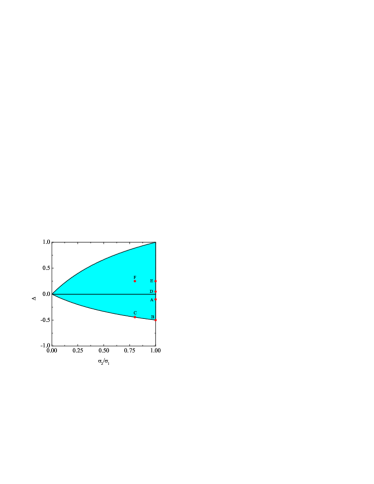
Figure 1: (Color online) Plane $\Delta$ vs $\sigma_{2}/\sigma_{1}$ showing the shaded region $-\sigma_{2}/(\sigma_{1}+\sigma_{2})\leq\Delta\leq 2\sigma_{2}/(\sigma_{1}+\sigma_{2})$ where the first two singularities of $g_{ij}(r)$, according to approximation RFA, are $\sigma_{ij}$ and $\sigma_{ik}-a_{kj}$ with $k\neq j$. The circles denote the systems analyzed in Sec. V.

Appendix C gives the expressions for $g_{ij}(r)$ in the range $0\leq r\leq\max(\sigma_{ij},\tau_{ij})+\epsilon$, where $\epsilon$ is any positive value smaller than the separation between $\max(\sigma_{ij},\tau_{ij})$ and the next singularity of $g_{ij}(r)$, provided by approximation RFA for binary mixtures. Extending to general $n$ the arguments presented there, we can write

$$G_{ij}(s)=e^{-\sigma_{ij}s}\Phi_{ij}(s)+2\pi\rho x_{\kappa}e^{-\tau_{ij}s}\Gamma_{i\kappa j}(s)+\cdots,$$ (70)

where $k=\kappa$ is the index corresponding to $\tau_{ij}$, i.e., $\tau_{ij}=\sigma_{i\kappa}-a_{\kappa j}$, and the ellipsis denotes terms headed by exponentials of the form $e^{-\lambda s}$ with $\lambda>\max(\sigma_{ij},\tau_{ij})$. In Eq. (70),

$$\Phi_{ij}(s)\equiv\frac{1}{s^{2}}L_{ij}(s)\bar{Q}_{jj}(s),$$ (71)

$$\Gamma_{ikj}(s)\equiv\frac{1}{s^{5}}\frac{L_{ik}(s)N_{kj}(s)}{D_{0}(s)},$$ (72)

where

$$\bar{Q}_{ij}^{-1}(s)\equiv\delta_{ij}-\frac{2\pi\rho\sqrt{x_{i}x_{j}}}{s^{3}}N_{ij}(s),$$ (73)

and $D_{0}(s)$ is the determinant of the matrix $\bar{\mathsf{Q}}^{-1}(s)$. Explicit expressions of $\Phi_{ij}(s)$ and $D_{0}(s)$ for binary mixtures are given in Appendix C.

Taking the Laplace inversion of Eq. (70), one finds that, in the interval $0\leq r\leq\max(\sigma_{ij},\tau_{ij})+\epsilon$,

$$g_{ij}(r) = \frac{1}{r}\Theta(r-\sigma_{ij})\phi_{ij}(r-\sigma_{ij})$$ (74)

$$+\frac{2\pi\rho}{r}x_{\kappa}\Theta(r-\tau_{ij})\gamma_{i\kappa j}(r-\tau_{ij}),$$

where $\phi_{ij}(r)$ and $\gamma_{ikj}(r)$ are the inverse Laplace transforms of $\Phi_{ij}(s)$ and $\Gamma_{ikj}(s)$, respectively.

Note that $\phi_{ij}(0)=\lim_{s\to\infty}\Phi_{ij}(s)=L_{ij}^{(1)}$, while $\gamma_{ikj}(0)=\lim_{s\to\infty}\Gamma_{ikj}(s)=0$. Therefore, the contact values are

$$g_{ij}(\sigma_{ij}^{+})=\frac{L_{ij}^{(1)}}{\sigma_{ij}}+\frac{2\pi\rho}{\sigma_{ij}}x_{\kappa}\Theta(\sigma_{ij}-\tau_{ij})\gamma_{i\kappa j}(\sigma_{ij}-\tau_{ij}).$$ (75)

As expected, Eq. (75) reduces to Eq. (40) in the additive case.

III.3 Approximation $\text{RFA}_{+}$

This new option for $g_{ij}(r)$ will differ from approximation RFA only in the region $\min(\sigma_{ij},\tau_{ij})\leq r\leq\max(\sigma_{ij},\tau_{ij})$. More specifically,

$$\left.g_{ij}(r)\right|_{\text{RFA}_{+}} = \left.g_{ij}(r)\right|_{\text{RFA}}+\frac{2\pi\rho}{r}x_{\kappa}\left[\Theta(r-\sigma_{ij})\right.$$ (76)

$$\left.-\Theta(r-\tau_{ij})\right]\gamma_{i\kappa j}(r-\tau_{ij}).$$

On account of Eq. (74), Eq. (76) can be equivalently rewritten as

$$\left.g_{ij}(r)\right|_{\text{RFA}_{+}}=\begin{cases}\Theta(r-\sigma_{ij})\left.g_{ij}(r)\right|_{\text{RFA}},\quad\tau_{ij}<\sigma_{ij},\\ \left.g_{ij}(r)\right|_{\text{RFA}}+\Theta(r-\sigma_{ij})\Theta(\tau_{ij}-r)\\ \quad\times\frac{2\pi\rho}{r}x_{\kappa}\gamma_{i\kappa j}(r-\tau_{ij}),\quad\tau_{ij}>\sigma_{ij}.\end{cases}$$ (77)

We see from Eq. (77) that the idea behind approximation $\text{RFA}_{+}$ is two-fold. On the one hand, it removes the unphysical violation of the property $g_{ij}(r)=0$ for $r<\sigma_{ij}$ that is present in option RFA when $\tau_{ij}<\sigma_{ij}$. On the other hand, if $\tau_{ij}>\sigma_{ij}$, approximation $\text{RFA}_{+}$ extrapolates to the region $\sigma_{ij}<r<\tau_{ij}$ the functional form of $g_{ij}(r)$ provided by approximation RFA in the region between $\tau_{ij}$ and the next singularity.

In the interval $0\leq r\leq\max(\sigma_{ij},\tau_{ij})+\epsilon$,

$$\left.g_{ij}(r)\right|_{\text{RFA}_{+}}=\frac{1}{r}\Theta(r-\sigma_{ij})[\phi_{ij}(r-\sigma_{ij})+{2\pi\rho}x_{\kappa}\gamma_{i\kappa j}(r-\tau_{ij})].$$ (78)

In particular,

$$\left.g_{ij}(\sigma_{ij}^{+})\right|_{\text{RFA}_{+}}=\frac{L_{ij}^{(1)}}{\sigma_{ij}}+\frac{2\pi\rho}{\sigma_{ij}}x_{\kappa}\gamma_{i\kappa j}(\sigma_{ij}-\tau_{ij}).$$ (79)

III.4 Approximation $\text{RFA}_{+}^{(m)}$

In approximation $\text{RFA}_{+}$ the full functional form of $\gamma_{ikj}(r)$ is used. This can create some artificial problems in the region $\sigma_{ij}<r<\tau_{ij}$ when $\tau_{ij}>\sigma_{ij}$ and the distance $\tau_{ij}-\sigma_{ij}$ is rather large (as happens in the WR model). Reciprocally, if $\tau_{ij}-\sigma_{ij}$ is not large, it becomes unnecessarily complicated to consider the entire nonlinear function $\gamma_{ikj}(r)$ in the interval $\sigma_{ij}<r<\tau_{ij}$. Thus, we now propose a variant of approximation $\text{RFA}_{+}$, here denoted as $\text{RFA}_{+}^{(m)}$, whereby the full true function $\gamma_{i\kappa j}(r)$ is preserved if $\tau_{ij}<\sigma_{ij}$ (in order to enforce the physical constraint of a vanishing RDF for $r<\sigma_{ij}$) but is replaced by its $m$th degree polynomial approximation $\gamma_{i\kappa j}^{(m)}(r)$ if $\tau_{ij}>\sigma_{ij}$. In summary, option $\text{RFA}_{+}^{(m)}$ is defined by

$$\left.g_{ij}(r)\right|_{\text{RFA}_{+}^{(m)}}=\begin{cases}\Theta(r-\sigma_{ij})\left.g_{ij}(r)\right|_{\text{RFA}},\quad\tau_{ij}<\sigma_{ij},\\ \left.g_{ij}(r)\right|_{\text{RFA}}+\Theta(r-\sigma_{ij})\Theta(\tau_{ij}-r)\\ \quad\times\frac{2\pi\rho}{r}x_{\kappa}\gamma_{i\kappa j}^{(m)}(r-\tau_{ij}),\quad\tau_{ij}>\sigma_{ij}.\end{cases}$$ (80)

Consequently, the contact values are

$$\left.g_{ij}(\sigma_{ij}^{+})\right|_{\text{RFA}_{+}^{(m)}} = \frac{L_{ij}^{(1)}}{\sigma_{ij}}+\frac{2\pi\rho}{\sigma_{ij}}x_{\kappa}$$ (81)

$$\times\Big{[}\Theta(\sigma_{ij}-\tau_{ij})\gamma_{i\kappa j}(\sigma_{ij}-\tau_{ij})$$

$$+\Theta(\tau_{ij}-\sigma_{ij})\gamma_{i\kappa j}^{(m)}(\sigma_{ij}-\tau_{ij})\Big{]}.$$

The polynomial $\gamma_{ikj}^{(m)}(r)$ is obtained by truncating after $r^{m}$ the expansion of $\gamma_{ikj}(r)$ in powers of $r$. Such an expansion is directly related to that of the Laplace transform $\Gamma_{ikj}(s)$ in powers of $s^{-1}$. For large $s$, $\Gamma_{ikj}(s)$ can be shown to be given by

$$\Gamma_{ikj}(s) = s^{-2}L_{ik}^{(1)}\left[L_{kj}^{(0)}\frac{b_{kj}}{2}-L_{kj}^{(1)}\right]b_{kj}+s^{-3}\Bigg{\{}L_{ik}^{(0)}\left[L_{kj}^{(0)}\frac{b_{kj}}{2}-L_{kj}^{(1)}\right]b_{kj}-L_{ik}^{(1)}\left[L_{kj}^{(0)}{b_{kj}}-L_{kj}^{(1)}\right]$$ (82)

$$+2\pi\rho L_{ik}^{(1)}\left[L_{kj}^{(0)}\frac{b_{kj}}{2}-L_{kj}^{(1)}\right]b_{kj}\sum_{\ell=1}^{n}x_{\ell}\left[L_{\ell\ell}^{(0)}\frac{\sigma_{\ell}}{2}-L_{\ell\ell}^{(1)}\right]\sigma_{\ell}\Bigg{\}}+\mathcal{O}(s^{-4}).$$

Consequently, the linear and quadratic approximations are

$$\gamma_{ikj}^{(1)}(r)=L_{ik}^{(1)}\left[L_{kj}^{(0)}\frac{b_{kj}}{2}-L_{kj}^{(1)}\right]b_{kj}{r},$$ (83)

$$\gamma_{ikj}^{(2)}(r) = \gamma_{ikj}^{(1)}(r)+\Bigg{\{}L_{ik}^{(0)}\left[L_{kj}^{(0)}\frac{b_{kj}}{2}-L_{kj}^{(1)}\right]b_{kj}-L_{ik}^{(1)}\left[L_{kj}^{(0)}{b_{kj}}-L_{kj}^{(1)}\right]$$ (84)

$$+2\pi\rho L_{ik}^{(1)}\left[L_{kj}^{(0)}\frac{b_{kj}}{2}-L_{kj}^{(1)}\right]b_{kj}\sum_{\ell=1}^{n}x_{\ell}\left[L_{\ell\ell}^{(0)}\frac{\sigma_{\ell}}{2}-L_{\ell\ell}^{(1)}\right]\sigma_{\ell}\Bigg{\}}\frac{r^{2}}{2}.$$

Of course, the three sets of approximations RFA, $\text{RFA}_{+}$, and $\text{RFA}_{+}^{(m)}$ reduce to the PY solution in the additive case. Obviously, $\text{RFA}_{+}\equiv\text{RFA}_{+}^{(\infty)}$. In Sec. V we will generally use $\text{RFA}_{+}^{(1)}$.

IV Comparison with Monte Carlo simulations for binary mixtures. The equation of state

The compressibility factor $Z$ is obtained via the virial and compressibility routes by Eqs. (7) and (13), respectively. In the case of the virial route one needs the contact values of the RDF, which are given by Eqs. (75), (79), and (81) in approximations RFA, $\text{RFA}_{+}$, and $\text{RFA}_{+}^{(m)}$, respectively.

In the compressibility route, the isothermal compressibility $\chi$ is obtained from Eq. (11), where $\widehat{h}_{ij}(0)=\rho\sqrt{x_{i}x_{j}}\widetilde{h}_{ij}(0)=-4\pi\rho\sqrt{x_{i}x_{j}}H_{ij}^{(1)}$, $H_{ij}^{(1)}$ being the coefficient of $s^{3}$ in the series expansion of $s^{2}G_{ij}(s)$ in powers of $s$ [cf. Eq. (33)]. We recall that $G_{ij}(s)$ is given by Eq. (47) in approximation RFA. In approximations $\text{RFA}_{+}$ and $\text{RFA}_{+}^{(m)}$, Eqs. (76) and (80) imply that

$$\left.H_{ij}^{(1)}\right|_{\text{RFA}_{+}}=\left.H_{ij}^{(1)}\right|_{\text{RFA}}-2\pi\rho x_{\kappa}\int_{\sigma_{ij}}^{\tau_{ij}}dr\,r\gamma_{i\kappa j}(r-\tau_{ij}),$$ (85)

$$\left.H_{ij}^{(1)}\right|_{\text{RFA}_{+}^{(m)}} = \left.H_{ij}^{(1)}\right|_{\text{RFA}}-2\pi\rho x_{\kappa}\int_{\sigma_{ij}}^{\tau_{ij}}dr\,r\Big{[}\Theta(\sigma_{ij}-\tau_{ij})$$

$$\times\gamma_{i\kappa j}(r-\tau_{ij})+\Theta(\tau_{ij}-\sigma_{ij})\gamma_{i\kappa j}^{(m)}(r-\tau_{ij})\Big{]}.$$

(86)

In any case, for the sake of simplicity, we will restrict ourselves in most of this section to approximation RFA.

IV.1 Dependence of the EOS on nonadditivity

Here we study the dependence of the EOS on the nonadditivity parameter $\Delta$ by fixing all the other parameters of the mixture (density, composition, and size ratio).

IV.1.1 Symmetric binary mixtures

Symmetric mixture are obtained when $\sigma_{1}=\sigma_{2}=\sigma$. Therefore, in the additive case ($\Delta=0$) one recovers the one-component HS system, i.e., $g_{11}(r)=g_{22}(r)=g_{12}(r)=g(r)$, regardless of the value of $x_{1}$.

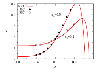
Figure 2: (Color online) Compressibility factor as a function of the nonadditivity parameter for a symmetric binary mixture of NAHSs at $\rho\sigma^{3}=0.2$ and two different compositions. The MC data are taken from Refs. Jung et al. (1994a, b).

Figure 2 compares the compressibility factor obtained from MC simulations Jung et al. (1994a, b) with that predicted by approximation RFA for some representative symmetric systems. We observe that approximation RFA reproduces quite well the exact simulation data at all values of the nonadditivity parameter. At this low density ($\rho\sigma^{3}=0.2,\eta\simeq 0.105$) the virial and compressibility routes are not distinguishable on the scale of the graph.

IV.1.2 Asymmetric binary mixtures

Asymmetric mixtures correspond to $\sigma_{1}\neq\sigma_{2}$. In that case, when $\Delta=0$ one recovers the AHS mixture.

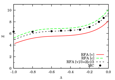
Figure 3: (Color online) Compressibility factor as a function of the nonadditivity parameter for an equimolar asymmetric binary mixture of NAHSs with a size ratio $\sigma_{2}/\sigma_{1}=1/3$ at a packing fraction $\eta=0.5$. The symbols [v] and [c] stand for the virial and compressibility routes, respectively. The MC data are taken from Ref. Hamad (1997).

Figure 3 shows the $\Delta$ dependence of $Z$ for negative nonadditivity and an equimolar ($x_{1}=x_{2}=\frac{1}{2}$) asymmetric mixture ($\sigma_{2}/\sigma_{1}=1/3$) at a relatively large density ($\eta=0.5$). In this case the virial route of approximation RFA underestimates the values of $Z$, while the compressibility route overestimates them. This is also a typical behavior of the PY equation for AHSs. It is thus tempting to try the $Z=\frac{1}{3}Z^{v}+\frac{2}{3}Z^{c}$ interpolation recipe Boublík (1970); Mansoori et al. (1971); Grundke and Henderson (1972); Lee and Levesque (1973), which is known to work well in the additive case. From Fig. 3 we see that indeed the interpolation formula, as applied to approximation RFA, reproduces quite well the exact simulation data, except for $\Delta\lesssim-0.8$.

IV.2 Dependence of the EOS on the size ratio

Next, we study the dependence of Z on the size ratio $\sigma_{2}/\sigma_{1}$ by fixing all the other parameters of the mixture (density, composition, and nonadditivity).

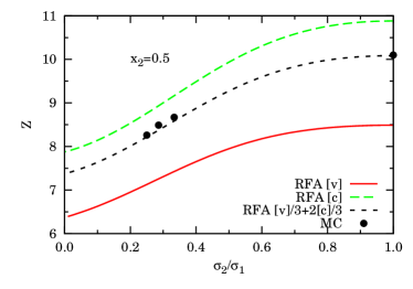
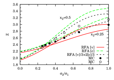
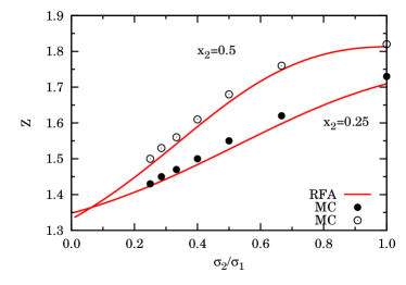
Figure 4: (Color online) Compressibility factor as a function of the size ratio $\sigma_{2}/\sigma_{1}$ for binary asymmetric NAHS mixtures with $x_{2}=\frac{1}{2}$, $\Delta=-0.05$, and $\eta=0.5$ (top panel); $x_{2}=\frac{1}{4},\frac{1}{2}$, $\Delta=0.2$, and $\eta=0.2$ (middle panel); $x_{2}=\frac{1}{4},\frac{1}{2}$, $\Delta=0.5$, and $\eta=0.075$ (bottom panel). In the bottom panel only the theoretical data obtained from the virial route are shown since they practically coincide with those obtained from the compressibility route. The MC data are taken from Ref. Hamad (1997).

The three panels of Fig. 4 show $Z$ vs $\sigma_{2}/\sigma_{1}$ for a slightly negative nonadditivity $\Delta=-0.05$ (top panel), a moderate positive nonadditivity $\Delta=0.2$ (middle panel), and a larger positive nonadditivity $\Delta=0.5$ (bottom panel). We observe again that the interpolation recipe $Z=\frac{1}{3}Z^{v}+\frac{2}{3}Z^{c}$ for approximation RFA agrees well with the exact simulation data, with the exception of a region close to the size symmetric mixture ($\sigma_{2}/\sigma_{1}=1$) for positive nonadditivity and moderate density (middle panel).

IV.3 Contact values

In Sec. V we will analyze the RDF $g_{ij}(r)$ predicted by approximations RFA and $\text{RFA}_{+}^{(1)}$. Before doing so, and as a bridge between the thermodynamic and structural properties, it is worth considering the contact values. Table 1 provides the contact values for some binary equimolar symmetric NAHS mixtures ($\sigma_{1}=\sigma_{2}=\sigma$, $x_{1}=x_{2}=\frac{1}{2}$), as obtained from MC simulations Ballone et al. (1986), numerical solutions of the PY integral equation Ballone et al. (1986), and our approximations RFA [Eq.  (75)] and $\text{RFA}_{+}^{(1)}$ [Eq.  (81)]. Since for binary symmetric mixtures $\tau_{11}=\tau_{22}=\sigma_{12}=\sigma(1+\Delta)$ and $\tau_{12}=\sigma$, it turns out that $g_{11}(\sigma^{+})=g_{22}(\sigma^{+})$ is common in approximations RFA and $\text{RFA}_{+}^{(1)}$ if $\Delta<0$, while $g_{12}(\sigma_{12}^{+})$ is common in both approximations if $\Delta>0$.

Table 1: Contact values for some binary equimolar symmetric NAHS mixtures. The MC and PY data were taken from Ref. Ballone et al. (1986). The labels correspond to systems common to those listed in Table 2.

Label	$\Delta$	$\rho\sigma^{3}$	Source	$g_{11}(\sigma^{+})$	$g_{12}(\sigma_{12}^{+})$
D	$0.05$	$0.8$	MC	$5.305$	$3.762$
			PY	$4.451$	$3.516$
			RFA	$4.006$	$3.617$
			$\text{RFA}_{+}^{(1)}$	$4.580$	$3.617$
	$0.0$	$0.8$	MC	$3.971$	$3.971$
			PY	$3.581$	$3.581$
			RFA	$3.581$	$3.581$
			$\text{RFA}_{+}^{(1)}$	$3.581$	$3.581$
	$-0.05$	$0.8$	MC	$3.117$	$3.801$
			PY	$2.925$	$3.394$
			RFA	$2.971$	$3.148$
			$\text{RFA}_{+}^{(1)}$	$2.971$	$3.445$
A	$-0.1$	$1.0$	MC	$3.394$	$5.363$
			PY	$3.209$	$4.395$
			RFA	$3.497$	$3.883$
			$\text{RFA}_{+}^{(1)}$	$3.497$	$4.763$
	$-0.3$	$1.0$	MC	$2.168$	$2.798$
			PY	$2.141$	$2.543$
			RFA	$2.441$	$2.251$
			$\text{RFA}_{+}^{(1)}$	$2.441$	$2.875$
B	$-0.5$	$1.0$	MC	$2.103$	$1.528$
			PY	$2.060$	$1.493$
			RFA	$2.139$	$1.407$
			$\text{RFA}_{+}^{(1)}$	$2.139$	$1.279$

From Table 1 we observe that approximation $\text{RFA}_{+}^{(1)}$ is superior to the PY theory in estimating the true contact values, both for positive and negative nonadditivity, except in the cases of $g_{11}(\sigma^{+})$ for $\rho\sigma^{3}=1$ and $\Delta=-0.3$ and of $g_{12}(\sigma_{12}^{+})$ for $\rho\sigma^{3}=1$ and $\Delta=-0.5$.

V Comparison with Monte Carlo simulations for binary mixtures. The structure

Table 2: The six binary NAHS mixtures considered in the analysis of the structure. The last column gives the compressibility factor as obtained from our MC simulations.

Label	$\sigma_{2}/\sigma_{1}$	$\Delta$	$x_{1}$	$\rho\sigma_{1}^{3}$	$\eta$	$Z_{\text{MC}}$
A	$1$	$-0.1$	$1/2$	$1.0$	$0.5236$	$8.648$
B	$1$	$-0.5$	$1/2$	$1.0$	$0.5236$	$3.429$
C	$4/5$	$-0.444$	$1/3$	$1.0$	$0.3533$	$2.335$
D	$1$	$0.05$	$1/2$	$0.8$	$0.4189$	$9.083$
E	$1$	$0.25$	$1/2$	$0.3$	$0.1571$	$2.556$
F	$4/5$	$0.25$	$1/3$	$0.3$	$0.1060$	$1.876$

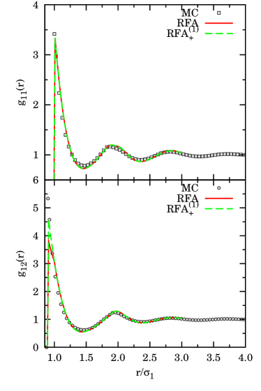
Figure 5: (Color online) RDF for system A of table 2.

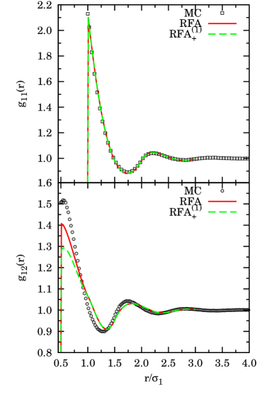
Figure 6: (Color online) RDF for system B of table 2.

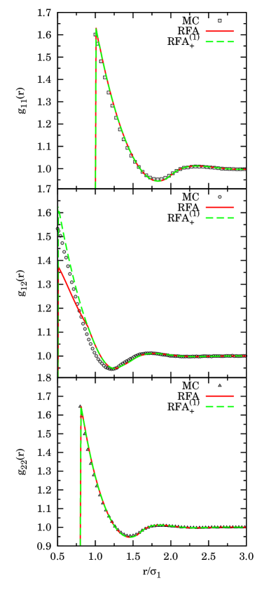
Figure 7: (Color online) RDF for system C of table 2.

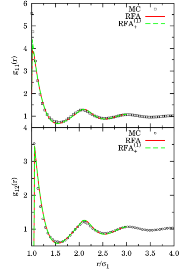
Figure 8: (Color online) RDF for system D of table 2.

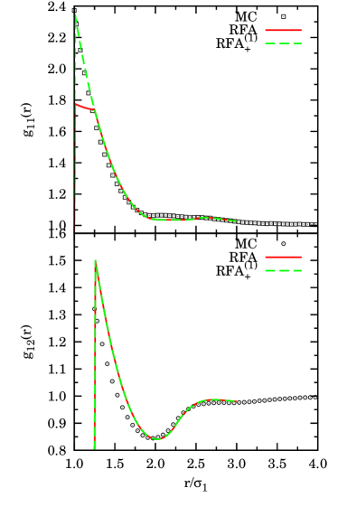
Figure 9: (Color online) RDF for system E of table 2.

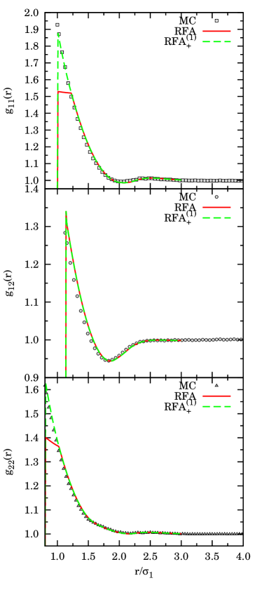
Figure 10: (Color online) RDF for system F of table 2.

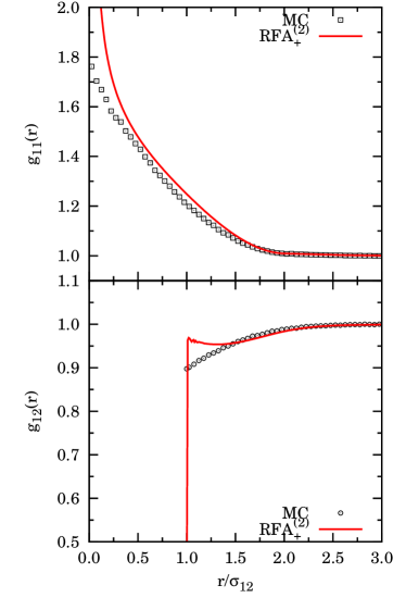
Figure 11: (Color online) RDF for the WR model at $\rho\sigma_{12}^{3}=0.28748$. The MC data are taken from Ref. Fantoni and Pastore (2004).

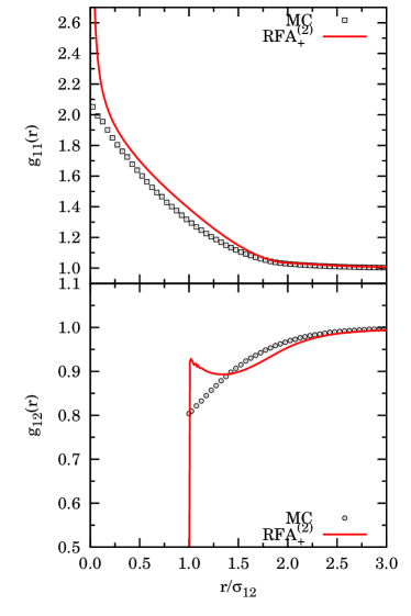
Figure 12: (Color online) RDF for the WR model at $\rho\sigma_{12}^{3}=0.4$. The MC data are taken from Ref. Fantoni and Pastore (2004).

The RDF of approximation RFA is analytically and explicitly given in Laplace space by Eqs. (47)–(49) and (58)–(64). In real space, $rg_{ij}(r)$ is easily found by taking the inverse Laplace transform of $G_{ij}(s)$ through the numerical scheme described in Ref. Abate and Whitt (1992). To get $g_{ij}(r)$ in approximation $\text{RFA}_{+}^{(m)}$, one needs to make use of Eq.  (80), where $\gamma_{ikj}^{(m)}(r)$ is explicitly given by Eqs. (83) and (84) for $m=1$ and $m=2$, respectively not . Notice that, while the true RDF has to be symmetric under exchange of species indices, the RDF obtained from approximation RFA or $\text{RFA}_{+}$ is, except for symmetric and equimolar mixtures, not symmetric, i.e., $g_{ij}(r)\neq g_{ji}(r)$ if $i\neq j$. Although this artificial asymmetry is generally small from a practical point of view, it represents a penalty we pay for our extension of the AHS solution of the PY equation. To cope with this shortcoming, we just redefine the like-unlike RDF as the symmetrized one $\frac{1}{2}[g_{ij}(r)+g_{ji}(r)]$.

In a binary mixture, $\tau_{11}=\sigma_{12}+a_{12}=\sigma_{1}+\frac{1}{2}(\sigma_{1}+\sigma_{2})\Delta$, $\tau_{22}=\sigma_{12}-a_{12}=\sigma_{2}+\frac{1}{2}(\sigma_{1}+\sigma_{2})\Delta$, and $\tau_{12}=\frac{1}{2}(\sigma_{1}+\sigma_{2})$. Therefore, $\tau_{11}<\sigma_{1}$ and $\tau_{22}<\sigma_{2}$ for $\Delta<0$, while $\tau_{12}<\sigma_{12}$ for $\Delta>0$. In what follows, we will truncate $\left.g_{ij}(r)\right|_{\text{RFA}}$ for $r<\sigma_{ij}$ when $\tau_{ij}<\sigma_{ij}$.

In order to evaluate the merits and limitations of the structural properties predicted by our approximations, we have performed canonical MC simulations of the binary NAHS system with $N=2196$ particles and $10^{5}N$ MC steps per run. The cell index method has been used Allen and Tildesley (1987). The statistical error on the RDF is within the size of the symbols used in the graphs reported.

We have chosen six representative systems, all within the region $-\sigma_{2}/(\sigma_{1}+\sigma_{2})\leq\Delta\leq 2\sigma_{2}/(\sigma_{1}+\sigma_{2})$ assumed in the construction of approximation $\text{RFA}_{+}$. Those six systems are represented in Fig. 1 and their respective values of composition and density are displayed in Table 2. Three of the mixtures have a negative nonadditivity (A, B, and C), while the other three have a positive nonadditivity (D, E, and F). Moreover, there are four equimolar symmetric mixtures (A, B, D, and E) and two asymmetric ones (C and F). In those two latter cases, however, both species contribute almost equally to the (nominal) packing fraction $\eta$ since $x_{1}\sigma_{1}^{3}/x_{2}\sigma_{2}^{3}=(5/4)^{3}/2=125/128\simeq 0.98$.

V.1 Negative nonadditivity

V.1.1 Symmetric mixtures

Figures 5 and 6 display the RDF for systems A and B, respectively. System A is only slightly nonadditive and we observe that both approximations RFA and $\text{RFA}_{+}^{(1)}$ do a very good job. On the other hand, while RFA and $\text{RFA}_{+}^{(1)}$ coincide for $g_{11}(r)$ with $r>\sigma_{1}$, they differ for $g_{12}(r)$ in the interval $\sigma_{12}=0.9\sigma_{1}\leq r\leq\tau_{12}=\sigma_{1}$. In fact, approximation RFA presents an artificial discontinuity of the first derivative $g_{12}^{\prime}(r)$ at $r=\sigma_{1}$. This is corrected by approximation $\text{RFA}_{+}^{(1)}$, which presents a good agreement with the MC results for $r<\sigma_{1}$. In spite of this, we observe that approximation $\text{RFA}_{+}^{(1)}$ underestimates the contact value $g_{12}(\sigma_{12}^{+})$, in agreement with the entry of Table 1 corresponding to case A.

In the case of system B the nonadditivity is larger and, according to Fig. 6, the performance of our approximations is still good for $g_{11}(r)$ but worsens for $g_{12}(r)$. In fact, $\left.g_{12}(r)\right|_{\text{RFA}}$ turns out to be better than $\left.g_{12}(r)\right|_{\text{RFA}_{+}^{(1)}}$ in the region $\sigma_{12}=0.5\sigma_{1}\leq r\leq\tau_{12}=\sigma_{1}$, in agreement with the entry of Table 1 corresponding to case B. In any case, it is interesting to remark that approximation $\text{RFA}_{+}^{(1)}$ succeeds in capturing the non-monotonic behavior of $g_{12}(r)$ very near $r=\sigma_{12}$ observed in the simulations.

V.1.2 Asymmetric mixture

The only case representing an asymmetric mixture with negative nonadditivity (system C) is shown in Fig. 7. Again, the MC like-like RDF are very well reproduced by the two approximations. In the case of the like-unlike function $g_{12}(r)$, approximation $\text{RFA}_{+}^{(1)}$ clearly improves approximation RFA in the region $\sigma_{12}=0.5\sigma_{1}\leq r\leq\tau_{12}=0.9\sigma_{1}$. Apart from that, both approximations overestimate $g_{12}(r)$ between $r=\tau_{12}=0.9\sigma_{1}$ and the location of the first minimum at about $r\simeq 1.25\sigma_{1}$. In Fig. 7 we have taken $g_{12}(r)\to\frac{1}{2}[g_{12}(r)+g_{21}(r)]$, as explained at the beginning of this section. Prior to this symmetrization, the maximum relative deviation between $g_{12}(r)$ and $g_{21}(r)$ occurs at $r\simeq 0.75\sigma_{1}$ and is less than 5%.

V.2 Positive nonadditivity

V.2.1 Symmetric mixtures

Let us consider now positive nonadditivities, starting with symmetric mixtures. Figures 8 and 9 show the results for systems D and E, respectively. For a small nonadditivity $\Delta=0.05$, both approximations provide very good results, except for $g_{11}(r)$ near contact (see also Table 1). Notice, however, that approximation $\text{RFA}_{+}^{(1)}$ improves approximation RFA in the narrow region $\sigma_{1}\leq r\leq\tau_{11}=1.05\sigma_{1}$.

For a larger nonadditivity (system E), Fig. 9 shows the excellent job made by approximation $\text{RFA}_{+}^{(1)}$ in the interval $\sigma_{1}\leq r\leq\tau_{11}=1.25\sigma_{1}$. In the case of the like-unlike correlation function, however, the approximations overestimate the values between $\sigma_{12}$ and the first minimum ($r\simeq 2\sigma_{1}$).

V.2.2 Asymmetric mixture

Figure 10 displays the three functions $g_{ij}(r)$ for the asymmetric system F. As in case E, approximation $\text{RFA}_{+}^{(1)}$ nicely reproduces the exact results from the simulation for the like-like correlations and corrects the unphysical kink of approximation RFA occurring at $\tau_{11}=1.225\sigma_{1}$ and $\tau_{22}=1.025\sigma_{1}$. Interestingly enough, although the values of $\Delta$ and $\rho\sigma_{1}^{3}$ are the same in systems E and F, the performance of the approximations for $g_{12}(r)$ is much better in case F (asymmetric mixture) than in case E (symmetric mixture). This might be partially due to the fact that the packing fraction $\eta$ is smaller in system F than in system E. For the asymmetric system F, we have found that the maximum relative deviation between $g_{12}(r)$ and $g_{21}(r)$ takes place at $r=\sigma_{12}=\frac{9}{8}\sigma_{1}$ and is less than $0.5$%.

V.3 The Widom–Rowlinson model

As recalled in Sec. I, the WR model corresponds to an equimolar symmetric binary NAHS mixture where $\sigma_{1}=\sigma_{2}=0$ and $\sigma_{12}\neq 0$. The model is then fully characterized by the reduced density, $\rho\sigma_{12}^{3}$. The critical demixing reduced density for this model is around $0.75$ Shew and Yethiraj (1996); Johnson et al. (1997).

The nonadditivity parameter of the WR model is $\Delta=\sigma_{12}/\sigma_{12}^{\text{add}}-1\to\infty$, so it lies well outside the “safe” region for our approximation $\text{RFA}_{+}$ (see Fig. 1). To compensate for this, we replace here approximation $\text{RFA}_{+}^{(1)}$ by approximation $\text{RFA}_{+}^{(2)}$.

We see from Figs.  11 and 12 that approximation $\text{RFA}_{+}^{(2)}$ does a much better job than expected at the two densities considered. The main drawbacks of the theory are that the contact value $g_{11}(0)$ is dramatically overestimated and the behavior of $g_{12}(r)$ for $r\gtrsim\sigma_{12}$ is qualitatively wrong. In spite of this, it is remarkable that approximation $\text{RFA}_{+}^{(2)}$ captures well the global properties of the RDF in this extreme system.

VI Summary and conclusions

The importance of the NAHS model in liquid state theory cannot be overemphasized. When the reference or effective interaction among the microscopic components (at an atomic or a colloidal level of description) of a statistical system is modeled as of hard-core type, there is no reason to expect that the interaction range $\sigma_{ij}$ corresponding to the pair $(i,j)$ is enslaved to be the arithmetic mean of the interaction ranges $\sigma_{i}$ and $\sigma_{j}$ corresponding to the pairs $(i,i)$ and $(j,j)$, respectively. Therefore, in an $n$-component NAHS mixture the number of independent interaction ranges is $n(n+1)/2$, in contrast to the number $n$ in an AHS mixture. It is then not surprising that, while an exact solution of the PY theory exists for AHS systems Lebowitz (1964), numerical methods are needed when solving the PY and other integral-equation theories for NAHSs Ballone et al. (1986). Therefore, analytical approaches to the problem can represent attractive and welcome contributions.

In this paper we have constructed a non-perturbative fully analytical approximation for the Laplace transforms $G_{ij}(s)$ of $rg_{ij}(r)$, where $g_{ij}(r)$ is the set of RDF of a general 3D NAHS fluid mixture. Our approach follows several stages. The starting point is the analytical PY solution for AHSs, Eqs. (36)–(38). Exploiting the connection between the exact solutions for 1D NAHS and AHS mixtures [see Eqs. (15) and (28)], the AHS PY solution is rewritten in an alternative form, Eqs. (44)–(47). Our approximation RFA consists of keeping the form (47), except that $\sigma^{\text{add}}_{ij}$ in Eq. (44) is replaced by $\sigma_{ij}$ [cf. Eq. (48)] and $\sigma_{i}$ in Eq. (46) is replaced by $b_{ij}\equiv\sigma_{ij}+a_{ij}$ [cf. Eq. (49)]. Moreover, the parameters $L_{ij}^{(0)}$ and $L_{ij}^{(1)}$ are no longer given by Eq. (41) but are determined by enforcing the condition (4) or, equivalently, Eq. (33). This results in Eqs. (58)–(64), and so the problem becomes completely closed and analytical in Laplace space. The equation of state is obtained either via the virial route (7) through the contact values (75) or via the compressibility route (11) through the coefficients $H_{ij}^{(1)}$ in the expansion of $s^{2}G_{ij}(s)$ in powers of $s$, Eq. (33).

The penalty we pay for “stretching” the AHS PY solution to the NAHS domain in the way described above is that $g_{ij}(r)$ may not be strictly zero for $r<\sigma_{ij}$ or may exhibit first-order discontinuities at artificial distances. To deal with this problem, we have restricted ourselves to mixtures such that the first two singularities of $g_{ij}(r)$ are $\sigma_{ij}$ and $\tau_{ij}\equiv\min(\sigma_{ik}-a_{kj};k=1,\ldots,n;k\neq j)$. In the binary case ($n=2$) this restriction corresponds to $-\sigma_{2}/(\sigma_{1}+\sigma_{2})\leq\Delta\leq 2\sigma_{2}/(\sigma_{1}+\sigma_{2})$ (see Fig. 1). Next, we have constructed a modified approximation $\text{RFA}_{+}$ whereby either $g_{ij}(r)$ is truncated for $r<\sigma_{ij}$ if $\tau_{ij}<\sigma_{j}$ or the behavior of $g_{ij}(r)$ for $r\gtrsim\tau_{ij}$ is extrapolated to the interval $\sigma_{ij}<r<\tau_{ij}$ if $\tau_{ij}>\sigma_{j}$ [cf. Eq. (77)]. From a practical point of view, the latter extrapolation can be replaced by a polynomial approximation (e.g., linear or quadratic), yielding approximation $\text{RFA}_{+}^{(m)}$ [cf. Eq. (80)]. This is sufficient to guarantee that the slope of $g_{ij}(r)$ is continuous everywhere for $r>\sigma_{ij}$.

For comparison with MC data of the equation of state we have used approximation RFA since its local limitations at the level of the RDF are largely smoothed out when focusing on the thermodynamic properties. The results show that, if the density is low enough as to make both thermodynamic routes practically coincide, our approximation accurately predicts the MC data, as shown in Fig. 2 and in the bottom panel of Fig. 4. For larger densities, the virial and compressibility routes tend to underestimate and overestimate, respectively, the simulation values, this being a typical PY feature. As in the AHS case, the simple interpolation rule $Z=\frac{1}{3}Z^{v}+\frac{2}{3}Z^{c}$ provides very good results, except for large nonadditivities (see Fig. 3 and the top and middle panels of Fig. 4).

Regarding the structural properties, approximation $\text{RFA}_{+}^{(1)}$ is found to perform quite well. The contact values are generally more accurate than those obtained from the numerical solution of the PY integral equation, at least for symmetric mixtures, as shown in Table 1. Comparison with our own MC simulations shows a very good agreement, except in the case of the like-unlike RDF for distances smaller than the location of the first minimum for large nonadditivities (cf. Figs. 5–10). On the other hand, even in the case of the WR model ($\Delta\to\infty$, well beyond the “safe” region of Fig. 1) our approximation $\text{RFA}_{+}^{(2)}$ does a much better job than expected, as illustrated in Figs. 11 and 12.

In conclusion, one can reasonably argue that our approximation RFA, along with its variants $\text{RFA}_{+}$ and $\text{RFA}_{+}^{(m)}$, represent excellent compromises between simplicity and accuracy. We have tried other alternative analytical approaches (simpler as well as more complex) also based on the PY solution for AHSs but none of them has been found to present a behavior as sound and consistent as those proposed in this paper. We expect that they can be useful in the investigation of such an important statistical-mechanical system (both by itself and also as a reference to other systems) as the NAHS mixture.

The work presented in this paper can be continued along several lines. In particular, we plan to explore in the near future the predictions for the demixing transition from our approximations. It is also worth exploring the NAHS theory that arises when the starting point is not the PY solution for AHSs but the more advanced RFA proposed in Ref. Yuste et al. (1998), which contains free parameters that can be accommodated to fit any desired EOS in a thermodynamically consistent way.

Appendix A Explicit expressions of $G_{ij}(s)$ for binary mixtures in approximation RFA

By performing the inversion of the matrix (51) and carrying out the matrix product in Eq. (47) one gets

$$G_{11}(s) = \frac{s^{-2}}{D(s)}\left\{L_{11}(s)\left[1-\frac{2\pi\rho x_{2}}{s^{3}}N_{22}(s)\right]e^{-\sigma_{1}s}\right.+\frac{2\pi\rho x_{2}}{s^{3}}L_{11}(s)L_{22}(s)e^{-(\sigma_{1}+\sigma_{2})s}$$ (87)

$$-\frac{2\pi\rho x_{2}}{s^{3}}L_{12}(s)L_{21}(s)e^{-2\sigma_{12}s}\left.+\frac{2\pi\rho x_{2}}{s^{3}}L_{12}(s)N_{21}(s)e^{-(\sigma_{12}+a_{12})s}\right\},$$

$$G_{12}(s)=\frac{s^{-2}}{D(s)}\left\{L_{12}(s)\left[1-\frac{2\pi\rho x_{1}}{s^{3}}N_{11}(s)\right]e^{-\sigma_{12}s}+\frac{2\pi\rho x_{1}}{s^{3}}L_{11}(s)N_{12}(s)e^{-(\sigma_{1}+\sigma_{2})s/2}\right\},$$ (88)

where the quadratic functions $N_{kj}(s)$ can be found in Eq. (52) and

$$D(s) = \left[1-\frac{2\pi\rho x_{1}}{s^{3}}N_{11}(s)\right]\left[1-\frac{2\pi\rho x_{2}}{s^{3}}N_{22}(s)\right]-\frac{(2\pi\rho)^{2}x_{1}x_{2}}{s^{6}}N_{12}(s)N_{21}(s)$$ (89)

$$+\frac{2\pi\rho x_{1}}{s^{3}}L_{11}(s)\left[1-\frac{2\pi\rho x_{2}}{s^{3}}N_{22}(s)\right]e^{-\sigma_{1}s}+\frac{2\pi\rho x_{2}}{s^{3}}L_{22}(s)\left[1-\frac{2\pi\rho x_{1}}{s^{3}}N_{11}(s)\right]e^{-\sigma_{2}s}$$

$$+\frac{4\pi^{2}\rho x_{1}x_{2}}{s^{6}}\left[L_{11}(s)L_{22}(s)e^{-(\sigma_{1}+\sigma_{2})s}-L_{12}(s)L_{21}(s)e^{-2\sigma_{12}s}\right.$$

$$\left.+L_{12}(s)N_{21}(s)e^{-(\sigma_{12}+a_{12})s}+L_{21}(s)N_{12}(s)e^{-(\sigma_{12}-a_{12})s}\right]$$

is the determinant of the matrix $\mathsf{Q}^{-1}$. The expressions for $G_{22}(s)$ and $G_{21}(s)$ can be obtained by the exchange $1\leftrightarrow 2$.

Appendix B Ordering of singular distances in approximation RFA for binary mixtures

By “singular” distances we will refer to those values of $r$ where the RDF $g_{ij}(r)$ or any of its derivatives have a discontinuity. Physical singularities are located, for instance, at $r=\sigma_{ij}$ and $r=\sigma_{ik}+\sigma_{kj}$, $k=1,\ldots,n$. Apart from that, approximation RFA introduces spurious singularities at other distances.

Let us particularize to a binary mixture. The physical leading singularity of $g_{ij}(r)$ should be located at $r=\sigma_{ij}$. However, according to Eq. (87), the leading singularity of $g_{11}(r)$ takes place at $r=\text{min}(\sigma_{1},\sigma_{12}+a_{12},2\sigma_{12})$. Analogously, the leading singularity of $g_{22}(r)$ is located at $r=\text{min}(\sigma_{2},\sigma_{12}-a_{12},2\sigma_{12})$. Finally, Eq. (88) shows that the leading singularity of $g_{12}(r)$ is $r=\frac{1}{2}\text{min}(2\sigma_{12},\sigma_{1}+\sigma_{2})$. Note that we have assumed $\sigma_{12}-a_{12}>0$, so that the denominator $D(s)$, Eq. (89), does not affect the leading singularity of $g_{ij}(r)$.

It is thus important to determine the relative ordering of the values $\sigma_{1}$, $\sigma_{2}$, $\sigma_{12}-a_{12}$, $\sigma_{12}+a_{12}$, $2\sigma_{12}$, and $\sigma_{1}+\sigma_{2}$. Such an ordering depends on the values of $\Delta$ and $R\equiv\sigma_{2}/\sigma_{1}$, where, without loss of generality, we assume that $\sigma_{2}\leq\sigma_{1}$. A detailed analysis shows that the $\Delta$-$R$ plane can be split into 13 disjoint regions with distinct order for the above singular distances. Those regions are indicated in Fig. 13, while Table 3 shows the order applying within each region. Note that $\sigma_{12}-a_{12}$ is negative in Regions IIf, IIg, and IIh, i.e., if $-1\leq\Delta\leq-2R/(1+R)$, thus invalidating those regions from the preceding analysis.

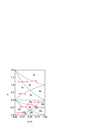
Figure 13: (Color online) Plane $\Delta$ vs $R\equiv\sigma_{2}/\sigma_{1}$ showing the regions with different ordering of the distances $\sigma_{1}$, $\sigma_{2}$, $\sigma_{12}-a_{12}$, $\sigma_{12}+a_{12}$, $2\sigma_{12}$, and $\sigma_{1}+\sigma_{2}$.

Table 3: Order of the singular distances $\sigma_{1}$, $\sigma_{2}$, $\sigma_{12}-a_{12}$, $\sigma_{12}+a_{12}$, $2\sigma_{12}$, and $\sigma_{1}+\sigma_{2}$ in each of the regions of Fig. 13.

Region	Order
Ia	$0$	$\leq$	$\sigma_{2}$	$\leq$	$\sigma_{12}-a_{12}$	$\leq$	$\sigma_{1}$	$\leq$	$\sigma_{12}+a_{12}$	$\leq$	$\sigma_{1}+\sigma_{2}$	$\leq$	$2\sigma_{12}$
Ib	$0$	$\leq$	$\sigma_{2}$	$\leq$	$\sigma_{1}$	$\leq$	$\sigma_{12}-a_{12}$	$\leq$	$\sigma_{12}+a_{12}$	$\leq$	$\sigma_{1}+\sigma_{2}$	$\leq$	$2\sigma_{12}$
Ic	$0$	$\leq$	$\sigma_{2}$	$\leq$	$\sigma_{12}-a_{12}$	$\leq$	$\sigma_{1}$	$\leq$	$\sigma_{1}+\sigma_{2}$	$\leq$	$\sigma_{12}+a_{12}$	$\leq$	$2\sigma_{12}$
Id	$0$	$\leq$	$\sigma_{2}$	$\leq$	$\sigma_{1}$	$\leq$	$\sigma_{12}-a_{12}$	$\leq$	$\sigma_{1}+\sigma_{2}$	$\leq$	$\sigma_{12}+a_{12}$	$\leq$	$2\sigma_{12}$
Ie	$0$	$\leq$	$\sigma_{2}$	$\leq$	$\sigma_{1}$	$\leq$	$\sigma_{1}+\sigma_{2}$	$\leq$	$\sigma_{12}-a_{12}$	$\leq$	$\sigma_{12}+a_{12}$	$\leq$	$2\sigma_{12}$
IIa	$0$	$\leq$	$\sigma_{12}-a_{12}$	$\leq$	$\sigma_{2}$	$\leq$	$\sigma_{12}+a_{12}$	$\leq$	$\sigma_{1}$	$\leq$	$2\sigma_{12}$	$\leq$	$\sigma_{1}+\sigma_{2}$
IIb	$0$	$\leq$	$\sigma_{12}-a_{12}$	$\leq$	$\sigma_{12}+a_{12}$	$\leq$	$\sigma_{2}$	$\leq$	$\sigma_{1}$	$\leq$	$2\sigma_{12}$	$\leq$	$\sigma_{1}+\sigma_{2}$
IIc	$0$	$\leq$	$\sigma_{12}-a_{12}$	$\leq$	$\sigma_{2}$	$\leq$	$\sigma_{12}+a_{12}$	$\leq$	$2\sigma_{12}$	$\leq$	$\sigma_{1}$	$\leq$	$\sigma_{1}+\sigma_{2}$
IId	$0$	$\leq$	$\sigma_{12}-a_{12}$	$\leq$	$\sigma_{12}+a_{12}$	$\leq$	$\sigma_{2}$	$\leq$	$2\sigma_{12}$	$\leq$	$\sigma_{1}$	$\leq$	$\sigma_{1}+\sigma_{2}$
IIe	$0$	$\leq$	$\sigma_{12}-a_{12}$	$\leq$	$\sigma_{12}+a_{12}$	$\leq$	$2\sigma_{12}$	$\leq$	$\sigma_{2}$	$\leq$	$\sigma_{1}$	$\leq$	$\sigma_{1}+\sigma_{2}$
IIf	$\sigma_{12}-a_{12}$	$\leq$	$0$	$\leq$	$\sigma_{2}$	$\leq$	$2\sigma_{12}$	$\leq$	$\sigma_{12}+a_{12}$	$\leq$	$\sigma_{1}$	$\leq$	$\sigma_{1}+\sigma_{2}$
IIg	$\sigma_{12}-a_{12}$	$\leq$	$0$	$\leq$	$2\sigma_{12}$	$\leq$	$\sigma_{2}$	$\leq$	$\sigma_{12}+a_{12}$	$\leq$	$\sigma_{1}$	$\leq$	$\sigma_{1}+\sigma_{2}$
IIh	$\sigma_{12}-a_{12}$	$\leq$	$0$	$\leq$	$2\sigma_{12}$	$\leq$	$\sigma_{12}+a_{12}$	$\leq$	$\sigma_{2}$	$\leq$	$\sigma_{1}$	$\leq$	$\sigma_{1}+\sigma_{2}$

We observe that $\sigma_{1}$ and $\sigma_{2}$ are indeed the leading singularities of $g_{11}(r)$ and $g_{22}(r)$, respectively, for positive nonadditivity (regions Ia–Ie). Reciprocally, $\sigma_{12}$ is the leading singularity of $g_{12}(r)$ for negative nonadditivity (regions IIa–IIh).

In order to construct approximation $\text{RFA}_{+}$, we want to restrict ourselves to those regions such that the two leading singularities of $g_{11}(r)$ are $\sigma_{1}$ and $\tau_{11}\equiv\sigma_{12}+a_{12}$. Inspection of Table 3 shows that Regions IIc–IIh are discarded by this criterion. In the remaining regions the leading singularity of $g_{11}(r)$ is $\text{min}(\sigma_{1},\sigma_{12}+a_{12})$ but the next one is not necessarily $\text{max}(\sigma_{1},\sigma_{12}+a_{12})$ since the latter value competes with $\text{min}(\sigma_{1},\sigma_{12}+a_{12})+\text{min}(\sigma_{2},\sigma_{12}-a_{12},2\sigma_{12})$, where the term $\text{min}(\sigma_{2},\sigma_{12}-a_{12},2\sigma_{12})$ comes from the denominator $D(s)$ [cf. Eq. (89)]. It can be checked that $\text{max}(\sigma_{1},\sigma_{12}+a_{12})\geq\text{min}(\sigma_{1},\sigma_{12}+a_{12})+\text{min}(\sigma_{2},\sigma_{12}-a_{12},2\sigma_{12})$ in Regions Ic–Ie. Therefore the two first singularities of $g_{11}(r)$ are $\sigma_{1}$ and $\tau_{11}=\sigma_{12}+a_{12}$ in Regions Ia, Ib, IIa, and IIb only. It turns out that in those four regions the two leading singularities of $g_{22}(r)$ are $\sigma_{2}$ and $\tau_{22}\equiv\sigma_{12}-a_{12}$, and the two leading singularities of $g_{12}(r)$ are $\sigma_{12}$ and $\tau_{12}\equiv\frac{1}{2}(\sigma_{1}+\sigma_{2})$.

In summary, Regions Ia, Ib, IIa, and IIb are the only ones where the two leading singularities of $g_{ij}(r)$ are $\sigma_{ij}$ and $\tau_{ij}\equiv\sigma_{ik}-a_{kj}$ with $k\neq j$.

Appendix C Short-range forms of $g_{ij}(r)$ for binary mixtures in approximation RFA

In what follows we assume that $-\sigma_{2}/(\sigma_{1}+\sigma_{2})\leq\Delta\leq 2\sigma_{2}/(\sigma_{1}+\sigma_{2})$, which corresponds to Regions Ia, Ib, IIa, and IIb of Fig. 13. As discussed in Appendix B, this guarantees that the first two singularities of $g_{ij}(r)$ are $\sigma_{ij}$ and $\tau_{ij}\equiv\sigma_{ik}-a_{kj}$ with $k\neq j$. The aim of this Appendix is to give the expressions of $g_{ij}(r)$ in the region $0\leq r\leq\max(\sigma_{ij},\tau_{ij})+\epsilon$, where $\epsilon$ is smaller than the separation between $\max(\sigma_{ij},\tau_{ij})$ and the next singularity.

It is convenient to assign a bookkeeping parameter $z$ to $e^{-s}$, so that, for instance, $e^{-\sigma_{ij}s}$ becomes $z^{\sigma_{ij}}e^{-\sigma_{ij}s}$. We will set $z=1$ at the end of the calculations. Therefore, the denominator $D(s)$ given by Eq. (89) becomes

$$D(s)=D_{0}(s)+o(z^{0}),$$ (90)

where

$$D_{0}(s) = \left[1-\frac{2\pi\rho x_{1}}{s^{3}}N_{11}(s)\right]\left[1-\frac{2\pi\rho x_{2}}{s^{3}}N_{22}(s)\right]$$ (91)

$$-\frac{(2\pi\rho)^{2}x_{1}x_{2}}{s^{6}}N_{12}(s)N_{21}(s).$$

In Eq. (90), $o(z^{n})$ denotes terms that are negligible versus $z^{n}$ in the (formal) limit $z\to 0$, i.e., $\lim_{z\to 0}z^{-n}o(z^{n})=0$. From Eq. (87) we see that the two leading terms in $G_{11}(s)$ are of orders $z^{\sigma_{1}}$ and $z^{\sigma_{12}+a_{12}}$:

$$G_{11}(s) = \Phi_{11}(s)e^{-\sigma_{1}s}z^{\sigma_{1}}+{2\pi\rho x_{2}}\Gamma_{121}(s)e^{-(\sigma_{12}+a_{12})s}$$ (92)

$$\times z^{\sigma_{12}+a_{12}}+o(z^{\sigma_{1}})+o(z^{\sigma_{12}+a_{12}}),$$

where

$$\Phi_{11}(s)\equiv\frac{s^{-2}}{D_{0}(s)}L_{11}(s)\left[1-\frac{2\pi\rho x_{2}}{s^{3}}N_{22}(s)\right]$$ (93)

and $\Gamma_{ikj}(s)$ is given by Eq. (72). Analogously,

$$G_{12}(s) = \Phi_{12}(s)e^{-\sigma_{12}s}z^{\sigma_{12}}+{2\pi\rho x_{1}}\Gamma_{112}(s)e^{-(\sigma_{1}+\sigma_{2})s/2}$$ (94)

$$\times z^{(\sigma_{1}+\sigma_{2})/2}+o(z^{\sigma_{12}})+o(z^{(\sigma_{1}+\sigma_{2})/2}),$$

$$G_{21}(s) = \Phi_{21}(s)e^{-\sigma_{12}s}z^{\sigma_{12}}+{2\pi\rho x_{2}}\Gamma_{221}(s)e^{-(\sigma_{1}+\sigma_{2})s/2}$$ (95)

$$\times z^{(\sigma_{1}+\sigma_{2})/2}+o(z^{\sigma_{12}})+o(z^{(\sigma_{1}+\sigma_{2})/2}),$$

$$G_{22}(s) = \Phi_{22}(s)e^{-\sigma_{2}s}z^{\sigma_{2}}+{2\pi\rho x_{1}}\Gamma_{212}(s)e^{-(\sigma_{12}-a_{12})s}$$ (96)

$$\times z^{\sigma_{12}-a_{12}}+o(z^{\sigma_{2}})+o(z^{\sigma_{12}-a_{12}}),$$

where

$$\Phi_{12}(s)\equiv\frac{s^{-2}}{D_{0}(s)}L_{12}(s)\left[1-\frac{2\pi\rho x_{1}}{s^{3}}N_{11}(s)\right],$$ (97)

$$\Phi_{21}(s)\equiv\frac{s^{-2}}{D_{0}(s)}L_{21}(s)\left[1-\frac{2\pi\rho x_{2}}{s^{3}}N_{22}(s)\right],$$ (98)

$$\Phi_{22}(s)\equiv\frac{s^{-2}}{D_{0}(s)}L_{22}(s)\left[1-\frac{2\pi\rho x_{1}}{s^{3}}N_{11}(s)\right].$$ (99)

Laplace inversion of Eqs. (92) and (94)–(96) shows that in the interval $0\leq r\leq\max(\sigma_{ij},\tau_{ij})+\epsilon$ we obtain

$$g_{11}(r) = \frac{1}{r}\Theta(r-\sigma_{1})\phi_{11}(r-\sigma_{1})+\frac{2\pi\rho x_{2}}{r}\Theta(r-\sigma_{12}-a_{12})$$ (100)

$$\times\gamma_{121}(r-\sigma_{12}-a_{12}),$$

$$g_{12}(r) = \frac{1}{r}\Theta(r-\sigma_{12})\phi_{12}(r-\sigma_{12})+\frac{2\pi\rho x_{1}}{r}\Theta(r-\frac{\sigma_{1}+\sigma_{2}}{2})$$ (101)

$$\times\gamma_{112}(r-\frac{\sigma_{1}+\sigma_{2}}{2}),$$

$$g_{21}(r) = \frac{1}{r}\Theta(r-\sigma_{21})\phi_{21}(r-\sigma_{12})+\frac{2\pi\rho x_{2}}{r}\Theta(r-\frac{\sigma_{1}+\sigma_{2}}{2})$$ (102)

$$\times\gamma_{221}(r-\frac{\sigma_{1}+\sigma_{2}}{2}),$$

$$g_{22}(r) = \frac{1}{r}\Theta(r-\sigma_{2})\phi_{22}(r-\sigma_{2})+\frac{2\pi\rho x_{1}}{r}\Theta(r-\sigma_{12}+a_{12})$$ (103)

$$\times\gamma_{212}(r-\sigma_{12}+a_{12}),$$

where we have already set $z=1$. In Eqs. (100)–(103), $\phi_{ij}(r)$ and $\gamma_{ikj}(r)$ are the inverse Laplace transforms of $\Phi_{ij}(s)$ and $\Gamma_{ikj}(s)$, respectively.

Since $\phi_{ij}(0)=\lim_{s\to\infty}\Phi_{ij}(s)=L_{ij}^{(1)}$, the contact values in approximation RFA are

$$g_{11}(\sigma_{1}^{+})=\frac{L_{11}^{(1)}}{\sigma_{1}},$$ (104)

$$g_{12}(\sigma_{12}^{+})=\frac{L_{12}^{(1)}}{\sigma_{12}}+\frac{2\pi\rho x_{1}}{\sigma_{12}}\gamma_{112}\left(\sigma_{12}-\frac{\sigma_{1}+\sigma_{2}}{2}\right),$$ (105)

$$g_{21}(\sigma_{12}^{+})=\frac{L_{21}^{(1)}}{\sigma_{12}}+\frac{2\pi\rho x_{2}}{\sigma_{12}}\gamma_{221}\left(\sigma_{12}-\frac{\sigma_{1}+\sigma_{2}}{2}\right),$$ (106)

$$g_{22}(\sigma_{2}^{+})=\frac{L_{22}^{(1)}}{\sigma_{2}},$$ (107)

in Regions Ia and Ib ($\Delta>0$). On the other hand, in Regions IIa and IIb ($\Delta<0$),

$$g_{11}(\sigma_{1}^{+})=\frac{L_{11}^{(1)}}{\sigma_{1}}+\frac{2\pi\rho x_{2}}{\sigma_{1}}\gamma_{121}\left(\sigma_{1}-\sigma_{12}-a_{12}\right),$$ (108)

$$g_{12}(\sigma_{12}^{+})=\frac{L_{12}^{(1)}}{\sigma_{12}},$$ (109)

$$g_{21}(\sigma_{12}^{+})=\frac{L_{21}^{(1)}}{\sigma_{12}},$$ (110)

$$g_{22}(\sigma_{2}^{+})=\frac{L_{22}^{(1)}}{\sigma_{2}}+\frac{2\pi\rho x_{1}}{\sigma_{2}}\gamma_{212}\left(\sigma_{2}-\sigma_{12}+a_{12}\right).$$ (111)

A more compact form is provided by Eq. (75).