Evolution in bouncing quantum cosmology

Abstract

We present the method of describing an evolution in quantum cosmology in the framework of the reduced phase space quantization of loop cosmology. We apply our method to the flat Friedman-Robertson-Walker model coupled to a massless scalar field. We identify the physical quantum Hamiltonian that is positive-definite and generates globally an unitary evolution of considered quantum system. We examine properties of expectation values of physical observables in the process of the quantum big bounce transition. The dispersion of evolved observables are studied for the Gaussian state. Calculated relative fluctuations enable an examination of the semi-classicality conditions and possible occurrence of the cosmic forgetfulness. Preliminary estimations based on the cosmological data suggest that there was no cosmic amnesia. Presented results are analytical, and numerical computations are only used for the visualization purposes. Our method may be generalized to sophisticated cosmological models including the Bianchi type universes.

1 Introduction

The loop quantum cosmology (LQC) method seems to be an efficient method of quantization of cosmological models of general relativity developed recently. Presently, we have two versions of this method: standard LQC (see, e.g. [1, 2, 3] and references therein) and nonstandard LQC [4, 5, 6, 7, 8, 9, 10, 11]. For an extended motivation for developing the nonstandard LQC we recommend an appendix of our paper [6].

The standard LQC has been developed by several groups around the world in the last decade. This approach follows the Dirac program in which one first identifies the kinematical Hilbert space ignoring the dynamical constraints. Next, the dynamical constraint (choosing suitable gauges leads to a single constraint) of the theory is promoted into an operator acting in this space. Kernel of this operator is used to construct the physical Hilbert space. Similarly, observables are analyzed firstly on the kinematical phase space and suitable unitary transformation is constructed to map the kinematical results into the physical ones.

The nonstandard LQC has been proposed recently. In the first stage of this approach one prepares the classical formalism for quantization: (1) Solutions to the Hamilton equations which satisfy the dynamical constraints are found. In the case of complicated system of equations, one may examine the structure of the constraint surface by the phase portrait methods for dynamical systems [12]. (2) Elementary Dirac observables on the constraint surface are determined, which define the physical phase space (PFS). (3) Physical observables are defined, i.e. the observables which after quantization can be used for predicting outcomes to be compared with observational data. Physical observables are introduced as functions of elementary Dirac observables and an evolution parameter. In the second stage, one quantizes the classical system: (1) Self-adjoint representations of physical observables are constructed by using the representation of the algebra of elementary observables. (2) Eigenvalue problems for physical observables are solved to get their spectra. (3) Evolution of expectation values of physical observables is examined. It consists in finding the new Hamiltonian of the classical theory that generates dynamics on the physical phase space. This new Hamiltonian is no longer a dynamical constraint of the classical theory. One finds a self-adjoint representation of this Hamiltonian. Quantum Hamiltonian is used, via Stone’s theorem, to define an unitary operator. This operator is used to examine an evolution of the quantum system.

Preliminary results obtained in [6, 11] indicate that proposed method of describing an evolution of a quantum cosmological system is reasonable. In this paper we give complete presentation of the evolution. We demonstrate that it is able to reveal the details concerning the nature of the quantum big bounce transition. In particular, we analyze quantum fluctuations of physical observables in the propagation across the quantum bounce from the past to the future time infinities.

In the standard LQC an evolution of cosmological system is described quite differently. The kernel equation for the operator constraint is used to construct, after some formal rearrangements, an equation interpreted as an evolution equation. Unfortunately, so obtained equation is usually so complicated that one can only solve it by combined analytical and numerical methods. This is why the preliminary examination of the evolution of the quantum FRW model has shown that classical big bang turns into quantum big bounce transition [3], but could not say anything specific about the nature of the quantum bounce. In particular, an evolution of the dispersion effects of quantum observables was not done satisfactory. Replacing an exact Hamiltonian constraint of the FRW model by a simpler one have enabled making some analytical analysis. This simplified method for describing an evolution, called sLQC [13], has shown that the cosmic amnesia for the case of semiclassical states, discovered earlier in analyzes of a simple cosmological toy model [14], does not occur [15].

Our nonstandard LQC method enables analytical studies, with an exact expression for dynamical constraints, of subtle quantum effects of specific cosmological model of the universe. In this paper, we consider the flat FRW model with a free massless scalar field. The choice of the model results from the fact that the dispersion effects have been examined so far mainly for this model. On the other hand, the model is quite simple and the FRW symmetry is supported by the current observational cosmology.

In order to have our paper self-contained, we recall in Sec. II A some aspects of derivation of the Hamiltonian constraint of our nonstandard LQC [8]. In Sec. II B we introduce the notion of the physical Hamiltonian. In Sec. III we construct the physical quantum Hamiltonian and examine its spectral properties. The evolution of quantum FRW model is presented in Sec. IV, where we consider the dispersion of physical observables. We also briefly evoke the problem of time. The relative fluctuations of observables, for the Gaussian state, are considered as a function of time in Sec. V. We conclude in the last section. Appendix A includes the derivation of the formulas used in the section on quantum fluctuations.

2 Classical dynamics

2.1 Hamiltonian constraint

The gravitational part of the classical Hamiltonian, in the Ashtekar variables $(A^{i}_{a},E^{a}_{i})$, is the sum of the first class constraints

$$H_{g}=\frac{1}{16\pi G}\int_{\Sigma}d^{3}{\bf x}(N^{i}C_{i}+N^{a}C_{a}+NC),$$ (1)

where $\Sigma$ is the space-like part of spacetime $\mathbb{R}\times\Sigma$, and where $C_{i}$ and $C_{a}$ denote the Gauss and the spatial diffeomorphisms constraints, respectively. For considered FRW model gauges are chosen in such a way that $C_{i}$ and $C_{a}$ constraints are automatically fulfilled. The only nontrivial part is the scalar constraint $C$ so the Hamiltonian reads

$$H_{g}=-\frac{1}{\gamma^{2}}\frac{1}{16\pi G}\int_{\Sigma}d^{3}{\bf x}\frac{1}{\sqrt{|\det E|}}E^{a}_{i}E^{b}_{j}\epsilon^{ij}_{k}F^{k}_{ab},$$ (2)

where $\gamma$ is the Barbero-Immirzi parameter, and where $F^{i}_{ab}$ is the curvature of $SU(2)$ connection $A^{i}_{a}$.

In LQC the gravitational degrees of freedom are parametrised by holonomies $h_{i}$ and fluxes $F_{i}$, which are functionals of the Ashtekar variables. These non-local functions are used to construct a non-perturbative theory. The holonomies and fluxes are the $SU(2)$ variables satisfying the holonomy-flux algebra. In the highly symmetric spaces, like the FRW model considered here, the forms of these functions are simple and known.

In particular, in the flat FRW model the flux may be parametrised by the $v$ variable and the holonomy is expressed in terms of the $\beta$ variable [6]. The variable $v$ is a physical volume defined as follows

$$v:=\int_{\mathcal{V}}dx_{1}dx_{2}dx_{3}\sqrt{det\,q_{ab}}=a^{3}\int_{\mathcal{V}}dx_{1}dx_{2}dx_{3}\sqrt{det\,q_{ab}^{0}}=:a^{3}\,V_{0},$$ (3)

where $\mathcal{V}\subset\Sigma$ is an elementary cell in the space with topology $\mathbb{R}^{3}$; $(x_{a})=(x^{a})=(x^{1},x^{2},x^{3})$ are Cartesian coordinates; $q_{ab}:=a^{2}\,q_{ab}^{0}$ is a physical 3-metric; $a$ is a scale factor; $q_{ab}^{0}dx^{a}dx^{b}:=dx_{1}^{2}+dx_{2}^{2}+dx_{3}^{2}$ defines a fiducial 3-metric; $V_{0}$ is a fiducial volume (it does not occur in final results). The $\beta$ variable, in the limit $\beta\rightarrow 0$, is linked to the Hubble factor $H=\dot{a}/a$ via the relation $\beta=\gamma H$.

In order to express the Hamiltonian, Eq. (2), in terms of holonomies and fluxes, the procedure of regularization has to be applied, which introduces a new scale to the theory, namely the parameter $\lambda$. This can be understood as the length scale of the lattice discretization. The applied procedure of regularization and rewriting the Hamiltonian in terms of holonomies and fluxes is the same as known from the standard LQC (see, Appendix A of [8]). The obtained gravitational part of the Hamiltonian reads [3]

$$H^{(\lambda)}_{g}=-\frac{vN}{32\pi^{2}G^{2}\gamma^{3}\lambda^{3}}\sum_{ijk}\epsilon^{ijk}\rm{tr}\left[h_{\Box_{ij}}h_{k}\left\{(h_{k})^{-1},v\right\}\right],$$

(4)

where $h_{\Box_{ij}}=h_{i}h_{j}(h_{i})^{-1}(h_{j})^{-1}$ is the holonomy around the square loop $\Box_{ij}$ (for more details see [5]), and $N$ is the lapse function. The elementary holonomy in the i-th direction reads

$$h_{i}=\cos\left(\frac{\lambda\beta}{2}\right)\mathbb{I}+2\sin\left(\frac{\lambda\beta}{2}\right)\tau_{i}$$ (5)

where $\tau_{i}=-\frac{i}{2}\sigma_{i}$ ($\sigma_{i}$ are the Pauli matrices). The holonomy (5) is calculated in the fundamental representation of $SU(2)$. The factor $\lambda$ is the parameter of the theory that may be related with the minimum area of the loop. It is expected that $\lambda\sim l_{\rm{Pl}}$, but its precise value has to be fixed observationally.

In the model considered in this paper, the total Hamiltonian is the sum of the gravity $H^{(\lambda)}_{g}$ and free scalar field $H_{\phi}:=Np^{2}_{\phi}/(2v)$ terms. The insertion of the elementary holonomy (5) into Eq. (4) leads (for details, see Appendix A of [8]) to the expression:

$$H^{(\lambda)}=N\left(-\frac{3}{8\pi l_{\rm{Pl}}^{2}\gamma^{2}}\frac{\sin^{2}(\lambda\beta)}{\lambda^{2}}v+\frac{p^{2}_{\phi}}{2v}\right)\approx 0,$$ (6)

where the sign “$\,\approx\,$” reminds that the Hamiltonian is a constraint of considered gravitational system.

The Hamilton equation takes the following form

$$\frac{df}{dt}=\{f,H^{(\lambda)}\},$$ (7)

where

$$\{\cdot,\cdot\}:=4\pi G\gamma\left[\frac{\partial\cdot}{\partial\beta}\frac{\partial\cdot}{\partial v}-\frac{\partial\cdot}{\partial v}\frac{\partial\cdot}{\partial\beta}\right]+\frac{\partial\cdot}{\partial\phi}\frac{\partial\cdot}{\partial p_{\phi}}-\frac{\partial\cdot}{\partial p_{\phi}}\frac{\partial\cdot}{\partial\phi}.$$ (8)

For the lapse function $N=1$ in Eq. (6), the time $t$ in equation (7) is the coordinate time. Using Eqs. (7) and (3) we get the expression for the Hubble factor, $H$, as follows

$$H:=\frac{\dot{a}}{a}=\frac{1}{3v}\frac{dv}{dt}=\frac{1}{\gamma}\frac{\sin(2\lambda\beta)}{2\lambda}.$$ (9)

We have the expansion period ($H>0$) for $\beta\in(0,\frac{\pi}{2\lambda})$, and the contraction ($H<0$) for $\beta\in(\frac{\pi}{2\lambda},\frac{\pi}{\lambda})$. The present classical phase of expansion corresponds to the limit $\beta\rightarrow 0$. In this limit, due to (9), we get $H=\beta/\gamma$. This relation can be also obtained from (9) by shrinking the regularization parameter $\lambda$ to zero.

The coordinate time $t$ used in cosmological observations and the intrinsic time (to be introduced later) preferred in theoretical considerations will be related via

$$\frac{d\phi}{dt}=\{\phi,H^{(\lambda)}\}=\frac{p_{\phi}}{v}.$$ (10)

Finding an explicit formula for $v$ in terms of $\phi$ (see next subsection) gives more insight into this relationship.

2.2 Physical Hamiltonian

The kinematical phase space $\mathcal{F}_{k}$ of the system can be parametrized by four independent variables $\beta,v,\phi,$ and $p_{\phi}$. If these variables satisfy the constraint (6), they can be used to parametrize the physical phase space $\mathcal{F}_{p}$ which is thus three dimensional. In the relative dynamics one canonical variable is used to parametrize all others. Choosing $\phi$ to play such a role enables an integration of the system and finding the elementary Dirac observables by the method presented in [5]:

$$\mathcal{O}_{1} = p_{\phi},$$ (11)

$$\mathcal{O}_{2} = \phi-\frac{\rm{sgn}(p_{\phi})}{\sqrt{12\pi}l_{\rm{Pl}}}\rm{arth}\left(\cos\left(\beta\lambda\right)\right),$$ (12)

$$\mathcal{O}_{3} = \rm{sgn}(p_{\phi})\ v\frac{\sin(\lambda\beta)}{\lambda},$$ (13)

which can be used to parametrize the phase space of the relative dynamics. Equations (11)-(13) take into account the constraint (6) so we have the relation [5]

$$\mathcal{O}_{3}=\kappa\gamma\mathcal{O}_{1},$$ (14)

where $\kappa^{2}:=4\pi G/3$. Thus, the physical phase space of the relative dynamics is two dimensional. It can be parametrized by two independent elementary observables, for instance $\mathcal{O}_{2}$ and $\mathcal{O}_{3}$.

The observables are constants of motions since, by the definition of Dirac’s observables, we have

$$\dot{\mathcal{{O}}}_{k}=\{\mathcal{O}_{k},H^{(\lambda)}\}=0,~{}~{}~{}~{}~{}~{}k=1,2,3.$$ (15)

Thus, acting with $d/d\phi$ on Egs. (11)-(13) leads to

$$0 = 1+\frac{\rm{sgn}(p_{\phi})}{\sqrt{12\pi}l_{\rm{Pl}}}\frac{\lambda}{\sin(\lambda\beta)}\frac{d\beta}{d\phi},$$ (16)

$$0 = \lambda\cos(\lambda\beta)\frac{d\beta}{d\phi}v+\sin(\lambda\beta)\frac{dv}{d\phi}.$$ (17)

We wish to emphasize again that (16) and (17) do include the constraint (6). In redefined variables

$$Q:=\beta,~{}~{}~{}~{}P:=\frac{1}{4\pi l_{\rm{Pl}}^{2}\gamma}v,~{}~{}~{}~{}T:=-\rm{sgn}(p_{\phi})\sqrt{3\pi}l_{\rm{Pl}}^{2}\phi,$$ (18)

equations (16) and (17) can be rewritten formally in the form

$$\frac{dP}{dT} = -\frac{\partial H_{\lambda}}{\partial Q},$$ (19)

$$\frac{dQ}{dT} = \frac{\partial H_{\lambda}}{\partial P},$$ (20)

where

$$H_{\lambda}:=\frac{2}{\lambda\sqrt{G}}P\sin(\lambda Q),$$ (21)

plays the role of the Hamiltonian of the system devoid of the dynamical constraint.

This way we have turned the system with constraint into the system without constraint. One can say that we have obtained the system in which the dynamical constraint has been solved.

Let us find the solution to the system defined by (19)-(21). By direct integrations, we find

$$Q=\frac{2}{\lambda}\arctan\exp\Big{(}\frac{2}{\sqrt{G}}(T-T_{0})\Big{)}.$$ (22)

Similarly, we get

$$P=P_{0}\cosh\Big{(}\frac{2}{\sqrt{G}}(T-T_{0})\Big{)},$$ (23)

where $P_{0}$ and $T_{0}$ are constants of integration.

The parameter $T$ is the intrinsic time for the relative dynamics under considerations. Using(10), (18) and (23) we relate this time with the coordinate time $t$:

$$t=t_{0}-2\sqrt{\frac{\pi G}{3}}\frac{\gamma P_{0}}{|p_{\phi}|}\sinh\Big{(}\frac{2}{\sqrt{G}}(T-T_{0})\Big{)}.$$ (24)

Since $P_{0}>0$ (as $P$ corresponds to the volume variable) and the r.h.s. of Eq. (24) monotonically decreasing with $T$, one can see that the directions of $t$ and $T$ are quite the opposite. Thus, the phase of expansion in coordinate time $t$ corresponds to the contraction phase in intrinsic time $T$ and vice versa. One can give the following interpretation: we define the Hubble parameter, $h$, in terms of the intrinsic time $T$, in analogy to (9), to get

$$h:=\frac{1}{3v}\frac{dv}{dT}=-\frac{2}{3}m_{\rm{Pl}}\cos(\lambda Q).$$ (25)

In contrast to the coordinate time case (9), we have a contraction ($h<0$) for $\;\lambda Q\in(0,\pi/2),\;$ and an expansion ($h>0$) for $\;\lambda Q\in(\pi/2,\pi)\;$. Using this we can say again that the directions of the intrinsic time $T$ and the coordinate time $t$ are the opposite.

It is commonly known that Hamiltonian of a physical physical system (being a part of some larger system) should be bounded from below, otherwise it would be dynamically unstable as the lowest energy state would not exist. It took much effort to prove that asymptotically flat spacetimes may have this property (see, e.g. the positive energy theorem [16]). In the case of cosmology, the situation is quite different since the system, being the entire universe, is not a part of some bigger system. In what follows we assume that our model of the universe is an isolated system. Since we consider a model which is a Hamiltonian system, its total energy must be conserved. Such a system (with fixed spacetime geometry and topology) cannot make transition to a state with lower or higher energy. The only reasonable requirement is that it should have finite value. However, our classical Hamiltonian, defined by (21), is positive-definite since $\lambda Q\in(0,\pi)$ and $P>0$, which enables reasonable interpretation of the model at the classical level. The values of $Q=0$ and $Q=\pi/\lambda$ can be approached by the classical trajectories only asymptotically. Owing to this, we postulate that the corresponding quantum Hamiltonian should be positive-definite too. At this stage we introduce the notion of the physical Hamiltonian. It is defined to be a positive-definite Hamiltonian that generates dynamics of the system. The property of being positive-definite is specific to our cosmological model and is devoid of basic importance.

The positivity of the Hamiltonian (21) was achieved by introducing an intrinsic time that has an opposite sine to the metric time. It is possible to redefine intrinsic time $T\rightarrow-T$, such that the directions of $T$ and $t$ will be the same. However, in such a case the Hamiltonian (21) would be multiplied by minus one so $H_{\lambda}$ no longer would be positive-definite.

The above reasoning presents the key ideas underlying the reduced phase space (RPS) approach of the classical level. In what follows we present the RPS quantization.

3 Quantum Hamiltonian

In what follows we use the Hilbert space $\mathcal{H}=L^{2}([0,\pi/\lambda],dQ)$ so it has the scalar product

$$\langle f|g\rangle:=\int_{0}^{\pi/\lambda}\overline{f}gdQ.$$ (26)

The quantum Hamiltonian corresponding to the classical one (21) is defined in a standard way to be

$$\hat{H}_{\lambda}:=\frac{m_{\rm{Pl}}}{\lambda}\left(\hat{P}\;\widehat{\sin(\lambda Q)}+\widehat{\sin(\lambda Q})\hat{P}\right).$$ (27)

The classical canonical variables $Q$ and $P$ satisfy the algebra $\{Q,P\}=1$. Choosing the Schrödinger representations for these variables

$$\hat{Q}\phi(Q):=Q\phi(Q),~{}~{}~{}~{}~{}\hat{P}\phi(Q):=-i\frac{d}{dQ}\phi(Q),$$ (28)

where $\phi\in\mathcal{H}$, gives formally $[\hat{Q},\hat{P}]=i\hat{\mathbb{I}}$.

An explicit form of the operator (27) is easily found to be

$$\hat{H}_{\lambda}\psi=-\frac{i}{\lambda\sqrt{G}}\left(2\sin(\lambda Q)\frac{d}{dQ}+\lambda\cos(\lambda Q)\right)\psi,$$ (29)

where $\psi\in D\subset\mathcal{H}$, and where $D$ is some dense subspace of $\mathcal{H}$. In what follows we wish to determine $D$ which is the domain of self-adjointness of the operator $\hat{H}_{\lambda}$.

3.1 Eigenproblem for the Hamiltonian

The eigenequation for the operator $\hat{H}_{\lambda}$ reads

$$-\frac{i}{\lambda\sqrt{G}}\left(2\sin(\lambda Q)\frac{d\Psi}{dQ}+\lambda\cos(\lambda Q)\Psi\right)=E\Psi.$$ (30)

The solution of the above equation is given by

$$\Psi_{E}=\Psi_{0}\frac{1}{\sqrt{\sin(\lambda Q)}}\exp\left\{\frac{1}{2}i\sqrt{G}E\ln\left|\tan\left(\frac{\lambda Q}{2}\right)\right|\right\},$$ (31)

where $\Psi_{0}$ is a constant of integration. Let us calculate

$$\langle\Psi_{E}|\Psi_{E^{\prime}}\rangle=|\Psi_{0}|^{2}\int_{0}^{\pi/\lambda}dQ\frac{\exp\left\{\frac{1}{2}i\sqrt{G}(E^{\prime}-E)\ln\left|\tan\left(\frac{\lambda Q}{2}\right)\right|\right\}}{\sin(\lambda Q)}.$$ (32)

Defining

$$x:=\frac{\sqrt{G}}{2}\ln\left|\tan\left(\frac{\lambda Q}{2}\right)\right|$$ (33)

once can rewrite the above integral into the form

$$\langle\Psi_{E}|\Psi_{E^{\prime}}\rangle = |\Psi_{0}|^{2}\frac{2}{\lambda\sqrt{G}}\int_{-\infty}^{+\infty}\exp\left\{i(E^{\prime}-E)x\right\}dx$$ (34)

$$= |\Psi_{0}|^{2}\frac{2}{\lambda\sqrt{G}}2\pi\delta(E^{\prime}-E).$$

By choosing

$$\Psi_{0}=\sqrt{\frac{\lambda\sqrt{G}}{4\pi}},$$ (35)

we get

$$\Psi_{E}(Q)=\langle Q|\Psi_{E}\rangle=\sqrt{\frac{\lambda\sqrt{G}}{4\pi\sin(\lambda Q)}}\exp\left\{\frac{1}{2}i\sqrt{G}E\ln\left|\tan\left(\frac{\lambda Q}{2}\right)\right|\right\}.$$ (36)

The states $\Psi_{E}$ given by equation (36) satisfies the orthonormality condition in the form

$$\langle\Psi_{E}|\Psi_{E^{\prime}}\rangle=\delta(E^{\prime}-E).$$ (37)

Based on this, for the eigenstates, we obtain

$$\langle\Psi_{E}|\hat{H}_{\lambda}\Psi_{E^{\prime}}\rangle-\langle\hat{H}_{\lambda}\Psi_{E}|\Psi_{E^{\prime}}\rangle=(E^{\prime}-E)\delta(E^{\prime}-E)=0,$$ (38)

which means that the Hamiltonian is symmetric on the space of the eigenstates.

3.2 Symmetricity

We define the domain of $\hat{H}_{\lambda}$ as follows

$$D(\hat{H}_{\lambda}):={\rm span}\{\varphi_{k},~{}~{}k\in\mathbb{Z}\},$$ (39)

where

$$\varphi_{k}(Q):=\int_{-\infty}^{\infty}c_{k}(E)\Psi_{E}(Q)\;dE,~{}~{}~{}c_{k}\in C^{\infty}_{0}(\mathbb{R}).$$ (40)

It is clear that $D(\hat{H}_{\lambda})\subset L^{2}([0,\pi/\lambda],dQ)=\mathcal{H}$ is a dense subspace of $\mathcal{H}$, and an action of the unbounded operator $\hat{H}_{\lambda}$ does not lead outside of $D(\hat{H}_{\lambda})$.

For any $\varphi_{k}$ and $\varphi_{l}$ we have

$$\langle\varphi_{k}|\hat{H}_{\lambda}\varphi_{l}\rangle-\langle\hat{H}_{\lambda}\varphi_{k}|\varphi_{l}\rangle=$$

$$=\int_{-\infty}^{+\infty}\int_{-\infty}^{+\infty}\overline{c_{k}(E)}c_{l}(E^{\prime})\underbrace{(E^{\prime}-E)\delta(E-E^{\prime})}_{=0}dEdE^{\prime}=0.$$ (41)

Therefore, the operator $\hat{H}_{\lambda}$ is symmetric on $D(\hat{H}_{\lambda})$.

3.3 Self-adjointness

To examine the self-adjointness of the unbounded operator $\hat{H}_{\lambda}$, we first identify the deficiency subspaces, $\mathcal{K_{\pm}}$, of this operator [18]

$$\mathcal{K_{\pm}}:=\{g_{\pm}\in D(\hat{H}_{\lambda}^{\ast})~{}|~{}\langle g_{\pm}|(\hat{H}_{\lambda}\pm i\mathbb{I})\varphi,\rangle=0,\;\forall\varphi\in D(\hat{H}_{\lambda}\},$$ (42)

where $D(\hat{H}_{\lambda}^{\ast}):=\{f\in L^{2}([0,\pi/\lambda],dQ)~{}|~{}\exists!f^{\ast}~{}\langle f^{\ast}|g\rangle=\langle f|\hat{H}_{\lambda}g\rangle,~{}\forall g\in D(\hat{H}_{\lambda})\}$, and where

$$f(Q):=\int_{-\infty}^{\infty}b(E)\Psi_{E}(Q)\;dE,~{}~{}~{}b\in C^{\infty}_{0}(\mathbb{R}).$$ (43)

For each $\varphi_{k}\in D(\hat{H}_{\lambda})$, defined by (40), we have

$$0 = \langle g_{\pm}|(\hat{H}_{\lambda}\pm i\mathbb{I})\varphi_{k}\rangle$$ (44)

$$= \int_{0}^{\pi/\lambda}dQ\int_{-\infty}^{\infty}dE_{1}\int_{-\infty}^{\infty}dE_{2}\;b_{\pm}^{\ast}(E_{2})\Psi_{E_{2}}^{\ast}(Q)(\hat{H}_{\lambda}\pm i\mathbb{I})c_{k}(E_{1})\Psi_{E_{1}}(Q)$$

$$= \int_{-\infty}^{\infty}dE_{1}\int_{-\infty}^{\infty}dE_{2}\;b_{\pm}^{\ast}(E_{2})c_{k}(E_{1})(E_{1}\pm i)\int_{0}^{\pi/\lambda}\Psi_{E_{2}}^{\ast}(Q)\Psi_{E_{1}}(Q)dQ$$

$$= \int_{-\infty}^{\infty}dE(E\pm i)b_{\pm}^{\ast}(E)c_{k}(E)~{}~{}~{}~{}\Longrightarrow~{}~{}~{}~{}~{}b_{+}=0=b_{-}.$$

Thus, the deficiency indices $n_{\pm}:=dim[\mathcal{K}_{\pm}]$ of $\hat{H}_{\lambda}$ satisfy the relation: $n_{+}=0=n_{-}$, which proves that the operator $\hat{H}_{\lambda}$ is essentially self-adjoint on $D(\hat{H}_{\lambda})$. One can argue that the whole spectrum of $\hat{H}_{\lambda}$ belongs to the real line.

3.4 Physical Hamiltonian

The classical physical Hamiltonian $H_{\lambda}$ is positive-definite. The corresponding self-adjoint operator $\hat{H}_{\lambda}$ has however eigenvalues $E\in\mathbb{R}$. We therefore introduce the quantum physical Hamiltonian $\hat{\mathbb{H}}$ by requiring that it has only positive eigenvalues. It is defined as follows

$$\hat{\mathbb{H}}|\Psi_{E}\rangle:=|E||\Psi_{E}\rangle,~{}~{}~{}~{}E>0,$$ (45)

where $|\Psi_{E}\rangle$ is the eigenvector of the Hamiltonian $\hat{H}$ corresponding to the eigenvalue $E$. It is clear that the spectrum of the operator $\hat{\mathbb{H}}$ is doubly degenerate. For any state $\Psi=\int_{-\infty}^{+\infty}c(E)\Psi_{E}\ dE\in D(\hat{\mathbb{H}})=D(\hat{H}_{\lambda})$, where $c\in C^{\infty}_{0}(\mathbb{R})$, we get

$$\langle\Psi|\hat{\mathbb{H}}|\Psi\rangle=\int_{-\infty}^{+\infty}dE|c(E)|^{2}|E|>0.$$ (46)

4 Evolution of quantum system

Making use of the Stone theorem [18], we define the unitary operator of an evolution as follows

$$\hat{U}(s):=e^{-is\hat{\mathbb{H}}},$$ (47)

where $s\in\mathbb{R}$ is a ‘time’ parameter. The state at any moment of time can be found as follows

$$|\Psi(s)\rangle=\hat{U}(s)|\Psi(0)\rangle=e^{-is\hat{\mathbb{H}}}|\Psi(0)\rangle.$$ (48)

The minus sign in (47), of the exponential function of an operator, is essential as only in this case an infinitesimal version of $\hat{U}(s)$ acting on $|\Psi(s)\rangle$ leads to the Schrödinger equation.

Let us consider a superposition of the Hamiltonian eigenstates

$$|\Psi(0)\rangle=\int_{-\infty}^{+\infty}dEc(E)|\Psi_{E}\rangle$$ (49)

at $s=0$. Then evolution of this state is given by

$$|\Psi(s)\rangle=\hat{U}(s)|\Psi(0)\rangle=\int_{-\infty}^{+\infty}dEc(E)e^{-is\hat{\mathbb{H}}}|\Psi_{E}\rangle$$

$$=\int_{-\infty}^{+\infty}dEc(E)e^{-is|E|}|\Psi_{E}\rangle.$$ (50)

Normalization of this state is given by the following condition

$$\langle\Psi(s)|\Psi(s)\rangle=\int_{-\infty}^{+\infty}\int_{-\infty}^{+\infty}dEdE^{\prime}\overline{c(E)}c(E^{\prime})e^{-is(|E|-|E^{\prime}|)}\underbrace{\langle\Psi_{E}|\Psi_{E^{\prime}}\rangle}_{=\delta(E^{\prime}-E)}$$

$$=\int_{-\infty}^{+\infty}dE|c(E)|^{2}=1.$$ (51)

Now, let us assume that the superposition (4) has a form of the Gaussian packet with the profile defined to be

$$c(E):=\left(\frac{2\alpha}{\pi}\right)^{1/4}e^{-\alpha\;(E-E_{0})^{2}},$$ (52)

centered around $E_{0}$ with the dispersion parametrized by $\alpha$.  The normalization factor $\left(2\alpha/\pi\right)^{1/4}$ is due to the condition (51). In the rest of this paper we study properties of this state only. Assuming that $E_{0}\sqrt{\alpha}\gg 1$, one can approximate

$$\Psi(Q,s) = \langle Q|\Psi(s)\rangle\left(\frac{2\alpha}{\pi}\right)^{1/4}\int_{-\infty}^{+\infty}dEe^{-\alpha(E-E_{0})^{2}-is|E|}\Psi_{E}(Q)$$ (53)

$$\simeq \left(\frac{2\alpha}{\pi}\right)^{1/4}\sqrt{\frac{\lambda\sqrt{G}}{4\pi\sin(\lambda Q)}}\int_{-\infty}^{+\infty}dEe^{-\alpha(E-E_{0})^{2}-isE}e^{iEx},$$

where $x:=\frac{1}{2}\sqrt{G}\ln\left|\tan\left(\frac{\lambda Q}{2}\right)\right|$. The approximation is valid because, for $E_{0}\sqrt{\alpha}\gg 1$, contribution from the negative energies to integral (53) is negligible. Therefore, $|E|$ can be replaced by $E$. Calculating the integral (53) we get

$$\Psi(Q,s)=\sqrt{\frac{\lambda}{\sqrt{8\pi\tilde{\alpha}}}}\frac{1}{\sqrt{\sin{(\lambda Q)}}}e^{-\frac{(x-s)^{2}}{4\alpha}}e^{iE_{0}(x-s)},$$ (54)

where $\tilde{\alpha}:=\alpha/G$. The probability density is easily found to be

$$\frac{|\Psi(Q,s)|^{2}}{\lambda}=\frac{\exp\left\{-\frac{1}{2\tilde{\alpha}}\left[\frac{1}{2}\ln\left|\tan\left(\frac{\lambda Q}{2}\right)\right|-\frac{s}{t_{\rm{Pl}}}\right]^{2}\right\}}{\sqrt{8\pi\tilde{\alpha}}\sin{(\lambda Q)}}.$$ (55)

It is worth to emphasis that the state (54) is normalizable so the probabilistic interpretation can be applied. Thus, the function $|\Psi(Q,s)|^{2}$ gives the probability density of finding universe with given $Q$ at the particular moment of time $s$. In the case $\lambda\rightarrow 0$, the state becomes non-normalizable and the probabilistic interpretation cannot be applied. Finding a normalizable state is a serious problem in most of quantum cosmologies different from LQC (see, e.g. [17]).

4.1 Evolution of observable $\hat{Q}$

One can now investigate the mean value of the $\hat{Q}$ operator in the $|\Psi(s)\rangle$ state. It is clear that $\hat{Q}$ is a symmetric bounded operator on $|\Psi(s)\rangle$. We find

$${\langle\hat{Q}\rangle}:=\langle\Psi(s)|\hat{Q}|\Psi(s)\rangle$$

$$=\frac{1}{\sqrt{2\pi\tilde{\alpha}}}\frac{2}{\lambda}\int_{-\infty}^{+\infty}\arctan\left\{\exp\left[2\left(y+\frac{s}{t_{\rm{Pl}}}\right)\right]\right\}\exp\left\{-\frac{1}{2\tilde{\alpha}}y^{2}\right\}dy.$$ (56)

One can show that

$$\lim_{s\rightarrow+\infty}\lambda\langle\hat{Q}\rangle(s)=\pi,~{}~{}~{}~{}~{}~{}\lim_{s\rightarrow-\infty}\lambda\langle\hat{Q}\rangle(s)=0,$$ (57)

which agrees with the classical limits. We also find

$$\langle\Psi(s)|\hat{Q}^{2}|\Psi(s)\rangle=$$

$$=\frac{1}{\sqrt{2\pi\tilde{\alpha}}}\left(\frac{2}{\lambda}\right)^{2}\int_{-\infty}^{+\infty}\arctan^{2}\left\{\exp\left[2\left(y+\frac{s}{t_{\rm{Pl}}}\right)\right]\right\}e^{-\frac{1}{2\tilde{\alpha}}y^{2}}dy.$$ (58)

Thus, the dispersion of $\hat{Q}$ in the state $|\Psi(s)\rangle$ reads

$$\Delta\hat{Q}:=\sqrt{\langle\Psi(s)|\hat{Q}^{2}|\Psi(s)\rangle-(\langle\Psi(s)|\hat{Q}|\Psi(s)\rangle)^{2}}.$$ (59)

In Fig. 1 we show ${\langle\hat{Q}\rangle}$ (thick blue line) and compare it with the classical solution (dashed red line)

$$Q=\frac{2}{\lambda}\arctan\exp\Big{(}\frac{2}{\sqrt{G}}(T-T_{0})\Big{)},$$ (60)

with $s=T-T_{0}$.

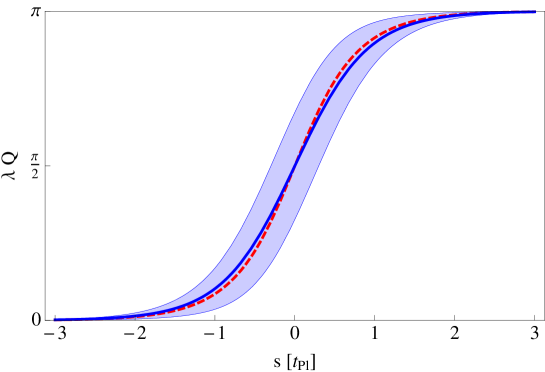
Figure 1: The thick blue line represents the mean value ${\langle\hat{Q}\rangle}$ for $\tilde{\alpha}=0.1$. The dashed red line is the classical solution $Q=\frac{2}{\lambda}\arctan\exp\left\{2s/t_{\rm{Pl}}\right\}$. The shadowed region is constrained by ${\langle\hat{Q}\rangle}\pm\Delta\hat{Q}$.

The shadowed region represents the dispersion of our state, and it is constrained by ${\langle\hat{Q}\rangle}\pm\Delta\hat{Q}$. One can notice that, close to the bounce at $s=0$ (where $\lambda Q=\pi/2$), the dispersion of the state is significant, while it fast decreases as $s\rightarrow\pm\infty$. Therefore, far from the bounce, the state converge to the classical solution.

4.2 Evolution of observable $\hat{P}$

The volume operator, due to (18), reads

$$\hat{v}=4\pi l_{\rm{Pl}}^{2}\gamma\hat{P}.$$ (61)

The $\hat{P}$ operator is unbounded, but symmetric on the state $|\Psi(s)\rangle$ defined by Eq. (54):

$$\langle\Psi(s)|\hat{P}\Psi(s)\rangle=-i\frac{\lambda}{\sqrt{8\pi\tilde{\alpha}}}\lim_{x\rightarrow+\infty}\cosh\left(\frac{2}{\sqrt{G}}x\right)\left[e^{-\frac{(x-s)^{2}}{2\alpha}}-e^{-\frac{(x+s)^{2}}{2\alpha}}\right]$$

$$+\langle\hat{P}\Psi(s)|\Psi(s)\rangle=\langle\hat{P}\Psi(s)|\Psi(s)\rangle,$$ (62)

where we used the relation $\cosh\left(\frac{2}{\sqrt{G}}x\right)=\frac{1}{\sin(\lambda Q)}$.

It is not difficult to derive the following:

$${\langle\hat{P}\rangle}:=\langle\Psi(s)|\hat{P}|\Psi(s)\rangle$$

$$=\frac{\lambda E_{0}}{\sqrt{8\pi\tilde{\alpha}}}\int_{-\infty}^{+\infty}\cosh\left(\frac{2}{\sqrt{G}}x\right)\exp\left\{-\frac{1}{2\alpha}(x-s)^{2}\right\}dx$$

$$=\frac{1}{2}\lambda E_{0}l_{\rm{Pl}}e^{2\tilde{\alpha}}\cosh\left(\frac{2s}{\sqrt{G}}\right).$$ (63)

Therefore,

$${\langle\hat{v}\rangle}=4\pi l_{\rm{Pl}}^{2}\gamma{\langle\hat{P}\rangle}=2\pi l_{\rm{Pl}}^{3}\gamma\lambda E_{0}e^{2\tilde{\alpha}}\cosh\left(\frac{2s}{\sqrt{G}}\right).$$ (64)

The minimum allowed volume in the $\Psi$ state is

$${\langle\hat{v}\rangle}_{\rm{min}}=2\pi l_{\rm{Pl}}^{3}\gamma\lambda E_{0}e^{2\tilde{\alpha}}.$$ (65)

The corresponding classical solution reads

$$v=v_{0}\cosh\Big{(}\frac{2}{\sqrt{G}}(T-T_{0})\Big{)}.$$ (66)

Thus, the functional forms of $\langle\hat{v}\rangle$ and $v$ coincide. We also find

$$\langle\Psi(s)|\hat{P}^{2}|\Psi(s)\rangle=\frac{\lambda^{2}}{32}\left[\left(\frac{1}{\tilde{\alpha}}-4+4\tilde{E}_{0}^{2}\right)\right.$$

$$+\left.\cosh\left(\frac{4s}{\sqrt{G}}\right)e^{8\tilde{\alpha}}\left(\frac{1}{\tilde{\alpha}}+4+4\tilde{E}_{0}^{2}\right)\right],$$ (67)

where $\tilde{E}_{0}:=E_{0}/E_{\rm{Pl}}$. The dispersion of $\hat{P}$ in the state $|\Psi(s)\rangle$ is found to be

$$\Delta\hat{P} := \sqrt{\langle\Psi(s)|\hat{P}^{2}|\Psi(s)\rangle-(\langle\Psi(s)|\hat{P}|\Psi(s)\rangle)^{2}}$$ (68)

$$= \frac{\lambda}{8}\left[2\left(\frac{1}{\tilde{\alpha}}-4+4\tilde{E}_{0}^{2}\right)+2\cosh\left(\frac{4s}{\sqrt{G}}\right)e^{8\tilde{\alpha}}\left(\frac{1}{\tilde{\alpha}}+4+4\tilde{E}_{0}^{2}\right)\right.$$

$$- \left.16\tilde{E}^{2}_{0}e^{4\tilde{\alpha}}\cosh^{2}\left(\frac{2s}{\sqrt{G}}\right)\right]^{1/2}$$

We visualize the dispersion of $\hat{P}$ as a function of time in Fig. 2.

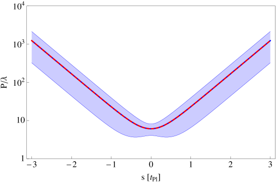
Figure 2: The thick blue line represents the mean value ${\langle\hat{P}\rangle}$ for $\tilde{\alpha}=0.1$ and $\tilde{E}_{0}=10$. The shadowed region is constrained by ${\langle\hat{P}\rangle}\pm\Delta\hat{P}$.

We can see that both the volume and its dispersion grow quite fast away (exponentially) from the big bounce region. This can be understood in the context of Heisenberg’s relation. Namely, while dispersion $\Delta\hat{Q}$ tends to zero, for $s\rightarrow\pm\infty$, the dispersion $\Delta\hat{P}$ grows appropriately to fulfill uncertainty relation $\Delta\hat{Q}\Delta\hat{P}\geq 1/2$. We shall study this issue in more details in the next subsection.

4.3 The Heisenberg uncertainty relation

The standard probabilistic interpretation of quantum mechanics cannot be applied to a cosmological system for a number of reasons. For instance, there is only one Universe and there is no observer outside the Universe. Thus, the process of measurement in quantum cosmology may differ from that known from the Copenhagen interpretation of quantum mechanics. Instead of complaining at the interpretation problems, it makes sense verification if some fundamental relations underlying quantum mechanics are satisfied. The best known is the Heisenberg uncertainty relation. What is its status in our cosmological setup? Is it satisfied during the quantum big bounce transition?

Our two canonical variables $\hat{Q}$ and $\hat{P}$ do not commute: $[\hat{Q},\hat{P}]=i\hat{\mathbb{I}}$. Since both operators are symmetric on the space of states $|\Psi(s)\rangle$, they should satisfy algebraically the Heisenberg relation:

$$\Delta\hat{Q}\;\Delta\hat{P}\geq 1/2.$$ (69)

In Fig. 3 we show the evolution of $\Delta\hat{Q}\Delta\hat{P}$ for the model considered in this paper.

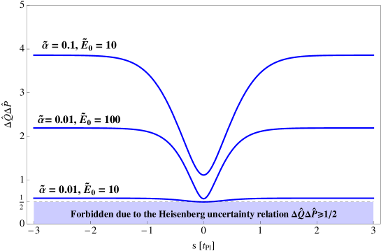
Figure 3: Evolution of the product of dispersions $\Delta\hat{Q}\Delta\hat{P}$. Heisenberg’s uncertainty relation $\Delta\hat{Q}\Delta\hat{P}\geq 1/2$ is preserved during the evolution.

We can see that the Heisenberg relation (69) is perfectly satisfied during the entire evolution, for any values of the parameters $\alpha$ and $E_{0}$ of the state. However, one cannot ascribe probabilistic interpretation to this relation. It is so because the representation $[\hat{Q},\hat{P}]=i\hat{\mathbb{I}}$ cannot be self adjoint owing to the fact (shown earlier) that $\hat{Q}$ and $\hat{P}$ are bounded and unbounded operators, respectively [19].

The function $\Delta\hat{Q}\Delta\hat{P}$ is symmetric with respect to the bounce and reaches its minimal value at the bounce. This is rather surprising result. Namely, one would expect that the transition point ($s=0$) is the most quantum part of the evolution, while in the limits $s\rightarrow\pm\infty$ one should get the most classical evolution. The situation is however quite the opposite. The transition point (big bounce) is the least quantum part of the evolution! In turn, in the limits $s\rightarrow\pm\infty$ the product of dispersions $\Delta\hat{Q}\Delta\hat{P}$ is saturated:

$$\lim_{s\rightarrow\pm\infty}\Delta\hat{Q}\Delta\hat{P}=$$

$$=\frac{1}{2}e^{4\tilde{\alpha}}\tilde{E}_{0}\sqrt{e^{4\tilde{\alpha}}-1}\sqrt{e^{4\tilde{\alpha}}-1+e^{4\tilde{\alpha}}\left(\frac{1}{4\tilde{E}_{0}^{2}\tilde{\alpha}}+\frac{1}{\tilde{E}_{0}^{2}}\right)}\geq\frac{1}{2},$$ (70)

which shows that the Gaussian packet we consider is always quantum. We can also see that the relation (70) does not depend on the parameter $\lambda$, which is a remarkable feature of our quantization scheme

Let us investigate in more details the value of $\Delta\hat{Q}\Delta\hat{P}$ at the bounce, $\Delta\hat{Q}\Delta\hat{P}|_{\rm{b}}$. In Fig. 4 we show $\Delta\hat{Q}\Delta\hat{P}|_{\rm{b}}$ as a function of $\tilde{\alpha}$ for $\tilde{E}_{0}=1,10$ and $100$.

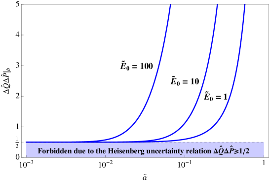
Figure 4: The value of $\Delta\hat{Q}\Delta\hat{P}$ at the bounce ($s=0$) as a function of the parameters of state.

As we can see, the boundary value $\Delta\hat{Q}\Delta\hat{P}|_{\rm{b}}=1/2$ is never crossed and it is approached for $\tilde{\alpha}\rightarrow 0$. Therefore, the more sharply peaked the state is, the smaller value of $\Delta\hat{Q}\Delta\hat{P}$ is at the bounce. For any value of $\tilde{\alpha}$, the smaller value of $\tilde{E}_{0}$ is the boundary $\Delta\hat{Q}\Delta\hat{P}|_{\rm{b}}=1/2$ is easier approached. In order to understand this dependence better, let us investigate separately $\Delta\hat{Q}|_{\rm{b}}$ and $\Delta\hat{P}|_{\rm{b}}$. We show these dispersions, as a function of $\tilde{\alpha}$, in the left and right panels of Fig. 5, respectively.

a)

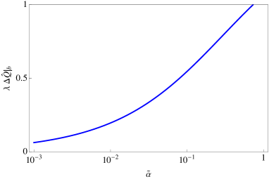
b)

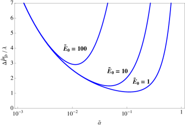
Figure 5: a) Dispersion $\lambda\Delta\hat{Q}$ at the bounce $(s=0)$ as a function of the parameter $\tilde{\alpha}$. b) Dispersion $\Delta\hat{P}/\lambda$ at the bounce $(s=0)$ as a function of the parameter $\tilde{\alpha}$ for $\tilde{E}_{0}=1,10$ and $100$.

The function $\Delta\hat{Q}|_{\rm{b}}$ grows monotonically with increase of $\tilde{\alpha}$ and is independent on $\tilde{E}_{0}$. The dependence on $\tilde{\alpha}$ is more complex for $\Delta\hat{P}|_{\rm{b}}$. Namely for any $\tilde{E}_{0}$ there always exists some $\tilde{\alpha}$ at which the function $\Delta\hat{P}|_{\rm{b}}(\tilde{\alpha})$ takes the minimum. The smallest possible value of $\Delta\hat{P}|_{\rm{b}}\approx 1.0686\lambda$ is reached for $\tilde{E}_{0}\rightarrow 0$ and $\tilde{\alpha}\approx 0.11797$.

In summary, our quantum cosmological setup is devoid of complete standard probabilistic interpretation, but satisfies formally the most basic relationships of the standard quantum mechanics.

4.4 Problem of time

An evolution of classical variables $Q$ and $P$, as presented by Eqs. (22) and (23), is parametrized by a free massless scalar field $\phi$, due to (18), that is a monotonic function so it can play the role of an internal clock [5]. The expectation values of the corresponding quantum operators $\hat{Q}$ and $\hat{P}$, defined by (47) and (63), are parametrized by $s\in\mathbb{R}$, owing to (47). Are the evolution variables $\phi$ and $s$ quite independent? An important difference between them is that they label an evolution of the system at different levels: classical and quantum, respectively. We postulate that these two variables are related linearly: $s=a_{1}\phi+a_{2},$ where $a_{1},a_{2}\in\mathbb{R}.$ It means that neither $\phi$ nor $s$ belong to the physical phase space. This seems to be the specific feature of our reduced phase space (RPS) method. It has been already proposed in [7] treating the $\phi$ variable as an evolution parameter of both classical and quantum dynamics. Such an interpretation is supported by the plots of Fig. 1 and Fig. 2, where the same abscissa is used to label both classical and quantum evolution of presented functions. The plots of classical and corresponding quantum functions practically coincide. Such an agreement suggests that our postulate concerning time variable is reasonable.

5 Relative fluctuations

In this section we study the relative fluctuations of the quantum observables $\hat{\mathcal{O}}$ in the state $|\Psi\rangle$. We consider three observables: $\hat{\mathbb{H}}$, $\hat{Q}$ and $\hat{P}$. The relative fluctuation $\Delta\hat{\mathcal{O}}/{\langle\hat{\mathcal{O}}\rangle}$ is a measure of the semi-classicality of a quantum state. We say that $|\Psi\rangle$ is semiclassical if $\;\Delta\hat{\mathcal{O}}/{\langle\hat{\mathcal{O}}\rangle}\ll 1$, and quantum if $\;\Delta\hat{\mathcal{O}}/\langle\hat{\mathcal{O}}\rangle\sim 1$. It is clear that the simiclassicality notion is not at all defined uniquely. We apply such a definition of semiclassicality because we wish to be able to make comparison of our analyzes with the available published results [14, 15, 20, 21, 22]. In the future we shall try to apply a more sophisticated definition: If the uncertainty in an observable is less than the observational precision, the state is semiclassical with respect to that observable.

In what follows, we also consider the function $D_{\mathcal{O}}$ characterizing the asymptotic aspects of relative fluctuations with respect to the bounce, defined to be [15]

$$D_{\mathcal{O}}:=\lim_{s\rightarrow\infty}\left[\left(\frac{\Delta\hat{\mathcal{O}}(-s)}{{\langle\hat{\mathcal{O}}\rangle}(-s)}\right)^{2}-\left(\frac{\Delta\hat{\mathcal{O}}(s)}{{\langle\hat{\mathcal{O}}\rangle}(s)}\right)^{2}\right].$$ (71)

5.1 Relative fluctuations of $\hat{\mathbb{H}}$

Let us start from deriving expectation value of $\hat{\mathbb{H}}$ in the state $|\Psi(s)\rangle$, we find

$${\langle\hat{\mathbb{H}}\rangle}:=\langle\Psi(s)|\hat{\mathbb{H}}|\Psi(s)\rangle=E_{0}\;\rm{erf}\left(\sqrt{2\alpha}E_{0}\right)+\frac{e^{-2\alpha E_{0}^{2}}}{\sqrt{2\pi\alpha}},$$ (72)

where $\rm{erf}(x):=\frac{2}{\sqrt{\pi}}\int_{0}^{x}e^{-t^{2}}dt$ is the error function. One can see that for $\sqrt{\alpha}E_{0}\gg 1$, the above expression simplifies to ${\langle\hat{\mathbb{H}}\rangle}\simeq E_{0}$. In order to find the dispersion of $\hat{\mathbb{H}}$, we also need:

$$\langle\Psi(s)|\hat{\mathbb{H}}^{2}|\Psi(s)\rangle=\frac{1}{4\alpha}+E_{0}^{2}.$$ (73)

Based on the above, we determine

$$\Delta\hat{\mathbb{H}}:=\sqrt{\langle\Psi(s)|\hat{\mathbb{H}}^{2}|\Psi(s)\rangle-(\langle\Psi(s)|\hat{\mathbb{H}}|\Psi(s)\rangle)^{2}}$$

$$=\left\{\frac{1}{4\alpha}+E_{0}^{2}\left[1-\rm{erf}^{2}\left(\sqrt{2\alpha}E_{0}\right)\right]\right.$$ (74)

$$\left.-\frac{2E_{0}e^{-2\alpha E_{0}^{2}}}{\sqrt{2\pi\alpha}}\rm{erf}\left(\sqrt{2\alpha}E_{0}\right)-\frac{e^{-4\alpha E_{0}^{2}}}{2\pi\alpha}\right\}^{1/2}.$$ (75)

We can see that for $\sqrt{\alpha}E_{0}\gg 1$, dispersion of $\hat{\mathbb{H}}$ simplifies to $\Delta\hat{\mathbb{H}}\simeq 1/\sqrt{4\alpha}$. Therefore, for $\sqrt{\alpha}E_{0}\gg 1$, the relative dispersion

$$\frac{\Delta\hat{\mathbb{H}}}{\langle\hat{\mathbb{H}}\rangle}\simeq\frac{1}{2\sqrt{\alpha}E_{0}}\ll 1.$$ (76)

It is worth to note that condition $\sqrt{\alpha}E_{0}\gg 1$ was also used while performing integration (53). One can see now that approximation based on this condition is justified by the restriction imposed on the relative fluctuations of the Hamiltonian $\hat{\mathbb{H}}$. The semiclassicality requires $\sqrt{\alpha}E_{0}\gg 1$. The relative fluctuations of $\hat{\mathbb{H}}$ are constant in time and therefore symmetric with respect to the bounce so finally we get: $D_{\mathbb{H}}=0$.

5.2 Relative fluctuations of $\hat{P}$

Relative fluctuations of $\hat{P}$ can be expressed as follows

$$\frac{\Delta\hat{P}}{\langle\hat{P}\rangle}=\sqrt{\frac{\left(\frac{1}{\tilde{\alpha}}-4+4\tilde{E}_{0}^{2}\right)+\cosh\left(\frac{4s}{\sqrt{G}}\right)e^{8\tilde{\alpha}}\left(\frac{1}{\tilde{\alpha}}+4+4\tilde{E}_{0}^{2}\right)}{8\tilde{E}_{0}^{2}e^{4\tilde{\alpha}}\cosh^{2}\left(\frac{2s}{\sqrt{G}}\right)}-1}.$$ (77)

In the left part of Fig. 6 we plot this relation for the different values of $\tilde{\alpha}$ and $\tilde{E}_{0}$.

a)

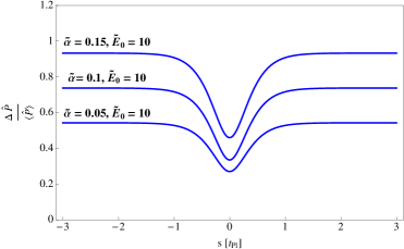
b)

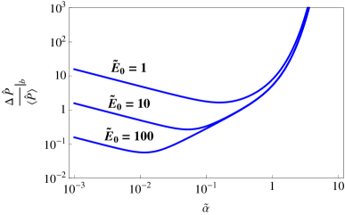
Figure 6: a) Relative fluctuations $\frac{\Delta\hat{P}}{{\langle\hat{P}\rangle}}$ for different values of $\tilde{\alpha}$ and $\tilde{E}_{0}$. b) Relative fluctuations $\frac{\Delta\hat{P}}{\langle\hat{P}\rangle}$ at the bounce ($s=0$) as a function of $\tilde{\alpha}$ for $\tilde{E}_{0}=1,10$ and $100$.

The relative fluctuations of $\hat{P}$ are symmetric with respect to the bounce and reach the minimal value at the transition point between the contracting and expanding phases. The symmetry $s\rightarrow-s$ directly implies that

$$D_{P}=\lim_{s\rightarrow\infty}\left[\left(\frac{\Delta\hat{P}(-s)}{{\langle\hat{P}\rangle}(-s)}\right)^{2}-\left(\frac{\Delta\hat{P}(s)}{{\langle\hat{P}\rangle}(s)}\right)^{2}\right]=0.$$ (78)

Thus, at infinite past and future times, the relative fluctuations of $\hat{P}$ are the same:

$$\left.\frac{\Delta\hat{P}}{\langle\hat{P}\rangle}\right|_{\rm{max}}=\lim_{s\rightarrow\pm\infty}\frac{\Delta\hat{P}}{\langle\hat{P}\rangle}=\sqrt{e^{4\tilde{\alpha}}-1+e^{4\tilde{\alpha}}\left(\frac{1}{4\tilde{E}_{0}^{2}\tilde{\alpha}}+\frac{1}{\tilde{E}_{0}^{2}}\right)}.$$ (79)

The function $\left.\frac{\Delta\hat{P}}{\langle\hat{P}\rangle}\right|_{\rm{max}}(\tilde{\alpha})$ has the minimum for any $\tilde{E}_{0}$, which is located at

$$\tilde{\alpha}_{\rm{min}}:=\frac{-1+\sqrt{5+4\tilde{E}_{0}^{2}}}{8(1+\tilde{E}_{0}^{2})}.$$ (80)

Therefore, having $\tilde{E}_{0}$, one can always minimize $\left.\frac{\Delta\hat{P}}{\langle\hat{P}\rangle}\right|_{\rm{max}}(\tilde{\alpha})$ by choosing $\tilde{\alpha}=\tilde{\alpha}_{\rm{min}}$. If $\tilde{E}_{0}\gg 1$, the expression (80) can be approximated by $\tilde{\alpha}_{\rm{min}}\approx 1/(4\tilde{E}_{0}).$

Let us now consider the fluctuations of $\hat{P}$ at the bounce, which can be expressed as follows

$$\left.\frac{\Delta\hat{P}}{\langle\hat{P}\rangle}\right|_{\rm{b}}=\sqrt{\frac{\left(\frac{1}{\tilde{\alpha}}-4+4\tilde{E}_{0}^{2}\right)+e^{8\tilde{\alpha}}\left(\frac{1}{\tilde{\alpha}}+4+4\tilde{E}_{0}^{2}\right)}{8\tilde{E}_{0}^{2}e^{4\tilde{\alpha}}}-1}.$$ (81)

We plot this function in the right part of Fig. 6 for fixed values of $\tilde{E}_{0}=1,10$ and $100$. As we can see, for any value of $\tilde{E}_{0}$, there is some $\tilde{\alpha}$ at which fluctuations take the minimum. These minimal value fluctuations decrease with the increase of $\tilde{E}_{0}$. In the limit $\tilde{E}_{0}\rightarrow\infty$, the relative fluctuations at the bounce are given by

$$\lim_{\tilde{E}_{0}\rightarrow\infty}\left.\frac{\Delta\hat{P}}{\langle\hat{P}\rangle}\right|_{\rm{b}}=\sqrt{2}\sinh(2\tilde{\alpha}).$$ (82)

Therefore, the fluctuations $\hat{P}$ at the bounce go to zero for $\tilde{\alpha}\rightarrow 0$ and $\tilde{E}_{0}\rightarrow\infty$.

5.3 Relative fluctuations of $\hat{Q}$

We have found (see, Appendix A) that after the bounce the relative fluctuations are decreasing and go to zero, so we have

$$\lim_{s\rightarrow+\infty}\frac{\Delta\hat{Q}(s)}{{\langle\hat{Q}\rangle}(s)}=0.$$ (83)

Therefore, the state becomes a semiclassical one. However, it may not be the case in the far past for large enough $\tilde{\alpha}$. While moving backward in time the relative fluctuations saturate. This saturated value can be found (see, Appendix B) by calculating the integrals: $\langle\Psi(s)|\hat{Q}|\Psi(s)\rangle$ and $\langle\Psi(s)|\hat{Q}^{2}|\Psi(s)\rangle$ . One gets

$$\left.\frac{\Delta\hat{Q}}{\langle\hat{Q}\rangle}\right|_{\rm{max}}=\lim_{s\rightarrow-\infty}\frac{\Delta\hat{Q}(s)}{{\langle\hat{Q}\rangle}(s)}=\sqrt{e^{4\tilde{\alpha}}-1},$$ (84)

where $\tilde{\alpha}>0$. Thus, before the bounce the state may be a quantum one if the value $\tilde{\alpha}$ is sufficiently large.

In Fig. 7 we present the plot of $\Delta\hat{Q}/{\langle\hat{Q}\rangle}$ for different values of $\tilde{\alpha}$.

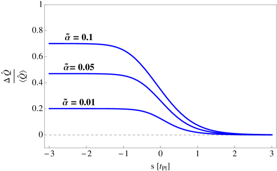
Figure 7: Relative fluctuations $\frac{\Delta\hat{Q}}{{\langle\hat{Q}\rangle}}$ for different values of $\tilde{\alpha}$

The relative fluctuations are not symmetric across the bounce ($s=0$). For $s\rightarrow+\infty$ the relative fluctuations converge to zero. For $s\rightarrow-\infty$ they saturate giving $\sqrt{e^{4\tilde{\alpha}}-1}$. The difference in the asymptotic values of the relative fluctuations is found to be

$$D_{Q}=e^{4\tilde{\alpha}}-1.$$ (85)

In order o interpret these results it is crucial to recall that directions of the parameter of time $s$ and coordinate time $t$ are opposite. Therefore, the positive values of $s$ correspond to contraction while negative to expansion. Therefore, the relative fluctuations of $\hat{Q}$ grow from the contracting to the expanding phase. So, the universe becomes more quantum with the increase of time $t$. The fluctuations tends to zero for $t\rightarrow-\infty$. Therefore the universe started its evolution from a sharply peaked state. Let us call it a semiclassical state. Only if the value of $\tilde{\alpha}$ is sufficiently small the universe will keep its semiclassicality during the whole evolution.

5.4 Semiclassicality

One can find that the maximal relative fluctuations of $\hat{P}$ and $\hat{Q}$ are related as follows

$$\left(\left.\frac{\Delta\hat{P}}{\langle\hat{P}\rangle}\right|_{\rm{max}}\right)^{2}=\left(\left.\frac{\Delta\hat{Q}}{\langle\hat{Q}\rangle}\right|_{\rm{max}}\right)^{2}+e^{4\tilde{\alpha}}\left(\frac{1}{4\tilde{E}_{0}^{2}\tilde{\alpha}}+\frac{1}{\tilde{E}_{0}^{2}}\right).$$ (86)

Thus, we have

$$\left.\frac{\Delta\hat{P}}{\langle\hat{P}\rangle}\right|_{\rm{max}}\geq\left.\frac{\Delta\hat{Q}}{\langle\hat{Q}\rangle}\right|_{\rm{max}}.$$ (87)

The equality is obtained in the limit ${\tilde{E}_{0}\rightarrow\infty}$, which leads to the equation:

$$\left.\frac{\Delta\hat{P}}{\langle\hat{P}\rangle}\right|_{\rm{max}}=\sqrt{e^{4\tilde{\alpha}}-1}=\left.\frac{\Delta\hat{Q}}{\langle\hat{Q}\rangle}\right|_{\rm{max}}.$$ (88)

It is clear that the semiclassicality condition

$$\left.\frac{\Delta\hat{P}}{\langle\hat{P}\rangle}\right|_{\rm{max}}\ll 1,$$ (89)

implicates, due to (87), that we have

$$\left.\frac{\Delta\hat{Q}}{\langle\hat{Q}\rangle}\right|_{\rm{max}}\ll 1.$$ (90)

Therefore, the semiclassicality imposed on $\hat{P}$ guaranties the semiclassicality for $\hat{Q}$. We can see that there is no cosmic forgetfulness if the condition (89) is satisfied.

The relation between maximal fluctuations $\left.\frac{\Delta\hat{P}}{\langle\hat{P}\rangle}\right|_{\rm{max}}$ and the fluctuations at the bounce $\left.\frac{\Delta\hat{P}}{\langle\hat{P}\rangle}\right|_{\rm{b}}$ is given by

$$\left(\left.\frac{\Delta\hat{P}}{\langle\hat{P}\rangle}\right|_{\rm{max}}\right)^{2}=\tanh(4\tilde{\alpha})+\frac{1}{\tilde{E}_{0}^{2}\cosh(4\tilde{\alpha})}+\frac{e^{4\tilde{\alpha}}}{\cosh(4\tilde{\alpha})}\left(\left.\frac{\Delta\hat{P}}{\langle\hat{P}\rangle}\right|_{\rm{b}}\right)^{2},$$ (91)

which leads to

$$\left.\frac{\Delta\hat{P}}{\langle\hat{P}\rangle}\right|_{\rm{max}}\geq\frac{e^{2\tilde{\alpha}}}{\sqrt{\cosh(4\tilde{\alpha})}}\left.\frac{\Delta\hat{P}}{\langle\hat{P}\rangle}\right|_{\rm{b}}.$$ (92)

Therefore, if the maximal fluctuations of $\hat{P}$ are constrained:

$$\left.\frac{\Delta\hat{P}}{\langle\hat{P}\rangle}\right|_{\rm{max}}\ll 1,$$ (93)

then we have

$$\left.\frac{\Delta\hat{P}}{\langle\hat{P}\rangle}\right|_{\rm{b}}\ll e^{-2\tilde{\alpha}}\sqrt{\cosh(4\tilde{\alpha})}\ll 1,$$ (94)

which proves (owing to $\left.\frac{\Delta\hat{Q}}{\langle\hat{Q}\rangle}\right|_{\rm{max}}\ll 1$, which implies $\alpha\ll 1$) that the bounce is semiclassical as well.

We have shown that condition $\left.\frac{\Delta\hat{P}}{\langle\hat{P}\rangle}\right|_{\rm{max}}\ll 1$ implies $\left.\frac{\Delta\hat{Q}}{\langle\hat{Q}\rangle}\right|_{\rm{max}}\ll 1$. Can this implication be true also in the opposite direction? The condition $\left.\frac{\Delta\hat{Q}}{\langle\hat{Q}\rangle}\right|_{\rm{max}}\ll 1$ it equivalent, due to (84), to the restriction $\tilde{\alpha}\ll 1$. By taking this into account, the maximal relative fluctuations of $\hat{P}$ can be expressed as follows

$$\left.\frac{\Delta\hat{P}}{\langle\hat{P}\rangle}\right|_{\rm{max}}=\frac{1}{2}\frac{1}{\sqrt{\tilde{\alpha}}\tilde{E}_{0}}+2\frac{\sqrt{\tilde{\alpha}}}{\tilde{E}_{0}}+\mathcal{O}(\tilde{\alpha}^{3/2}).$$ (95)

The first term in this expansion grows rapidly with decrease of $\tilde{\alpha}$. Therefore, unless the value of $\tilde{E}_{0}$ is not sufficiently large, the condition $\left.\frac{\Delta\hat{P}}{\langle\hat{P}\rangle}\right|_{\rm{max}}\ll 1$ is not fulfilled. This condition is fulfilled if $\tilde{E}_{0}\gg 1/\sqrt{\tilde{\alpha}}$, but this is exactly requirement of the semiclassicality of the relative fluctuations of $\hat{\mathbb{H}}$. Therefore, if the condition (76) is fulfilled, we have the equivalence:

$$\left(\left.\frac{\Delta\hat{P}}{\langle\hat{P}\rangle}\right|_{\rm{max}}\ll 1\right)\ \Longleftrightarrow\ \left(\left.\frac{\Delta\hat{Q}}{\langle\hat{Q}\rangle}\right|_{\rm{max}}\ll 1\right).$$ (96)

To complete our considerations, we show that the saturated value of $\Delta\hat{Q}\Delta\hat{P}$ can be easily expressed in terms of maximal relative fluctuations of $\hat{Q}$ and $\hat{P}$:

$$\lim_{s\rightarrow\pm\infty}\Delta\hat{Q}\Delta\hat{P}=\frac{1}{2}e^{4\tilde{\alpha}}\tilde{E}_{0}\left.\frac{\Delta\hat{Q}}{\langle\hat{Q}\rangle}\right|_{\rm{max}}\left.\frac{\Delta\hat{P}}{\langle\hat{P}\rangle}\right|_{\rm{max}}\geq\frac{1}{2}.$$ (97)

Owing to Heisenberg’s uncertainty relation, the above expression leads to the following constraint

$$\left.\frac{\Delta\hat{Q}}{\langle\hat{Q}\rangle}\right|_{\rm{max}}\left.\frac{\Delta\hat{P}}{\langle\hat{P}\rangle}\right|_{\rm{max}}\geq\frac{e^{-4\tilde{\alpha}}}{\tilde{E}_{0}}.$$ (98)

This constraint, together with inequality (87), results gives

$$\left.\frac{\Delta\hat{P}}{\langle\hat{P}\rangle}\right|_{\rm{max}}\geq\frac{e^{-2\tilde{\alpha}}}{\sqrt{\tilde{E}_{0}}}.$$ (99)

Thus, the samiclassicality condition (89) leads to the following constraint:

$$\tilde{E}_{0}\gg e^{-2\tilde{\alpha}}.$$ (100)

5.5 Forgetfulness

Let us try to answer the question: Was the Universe quantum or semiclassical before the big bounce? This question is related to the problem of cosmic forgetfulness discussed recently in papers [14, 15, 20, 21, 22]. If the Universe was quantum before the big bounce and the bounce transition turned it into semiclassical one, we can talk about a sort of cosmic amnesia. In this case the complete information about the Universe before the bounce cannot be obtained from the observational data after the bounce.

The above question has been addressed so far mainly by an examination of the relative fluctuations of the volume observable $\hat{v}$ (proportional to our $\hat{P}$ observable) [21, 22]. However, as we have shown, this type of fluctuation is symmetric with respect to the bounce. Therefore, the constraint on relative fluctuation at some time $+|s|$ results with the same constraint on the fluctuations at the time $-|s|$. As one can see on Fig. 6, the fluctuations of $\hat{P}$ saturate quickly outside the neighborhood of the bounce (within a few Planck’s times). Thus, present cosmic observation of the semiclassicality, $\frac{\Delta\hat{P}}{\langle\hat{P}\rangle}=\frac{\Delta\hat{v}}{\langle\hat{v}\rangle}\ll 1$, of the Universe would guarantee its semiclassicality in the distant past before the bounce. However, the situation is that this type of relative fluctuation cannot be ‘measured’. The reason is that one does not know, first of all, how to measure the ${\langle\hat{v}\rangle}$ quantity. It could be possible to measure the volume, to some extent, if the Universe was curved and the curvature term was measured in astronomical observations. At present, there is however no indication for such a contribution. Therefore, the fluctuations of $\hat{v}$ are not measurable so the cosmic forgetfulness cannot be examined by using the relative fluctuations $\frac{\Delta\hat{v}}{\langle\hat{v}\rangle}$.

What about the $\hat{Q}$ observable? The variable $Q$ is directly related to the expansion rate, i.e. the Hubble factor (9), which is a quantity that can be determined observationally. Thus, the value of $\langle\hat{Q}\rangle$ can be measured. Also the observational uncertainty of the Hubble factor can be used to constrain $\Delta\hat{Q}$. Therefore, relative fluctuations of $\hat{Q}$ can be constrained observationally! The present value of the Hubble factor is $H_{0}=70.2\pm 1.4\ \rm{km}\ \rm{s}^{-1}\ \rm{Mpc}^{-1}$ [23], therefore $\frac{\sigma(H_{0})}{H_{0}}\approx 0.02$. As we have shown in Sec. II, in the classical limit $Q=\gamma H$. Thus, we propose to consider the constraint: $\frac{\Delta\hat{Q}}{\langle\hat{Q}\rangle}<0.02$. This is because the relative quantum fluctuations cannot be greater than the relative uncertainty of measurement.

Due to the relation (24), the directions of the intrinsic time $T$ and the coordinate time $t$ are the opposite. Therefore, relative fluctuations of $\hat{Q}$ at $T\rightarrow-\infty$ correspond to the limit $t\rightarrow+\infty$. Thus, the relative fluctuations of $\hat{Q}$ grow in the coordinate time $t$ and saturate at $\sqrt{e^{4\tilde{\alpha}}-1}$. The model we consider is applicable to the evolution in vicinity of the Planck epoch. However, if we assume that the relative fluctuations behave similarly threafter, the present restriction $\frac{\Delta\hat{Q}}{\langle\hat{Q}\rangle}<0.02$ can be used to constraint the model. The condition $\sqrt{e^{4\tilde{\alpha}}-1}<0.02$ translates into the condition $\tilde{\alpha}<10^{-4}$. If the Gaussian state with such value of its parameter can be treated as a semiclassical one, we can say that the amnesia does not occur. In such a case the contraction and the bounce phases are semiclassical, so we have the cosmic recall.

The above constrains are quite preliminary. There exist the possibility to put more robust constraints based on the phase of inflation and observations of the Cosmic Microwave Background Radiation. However, for this purpose the model has to be generalized by taking into account potential of the scalar field.

6 Summary and Conclusions

In the Hamiltonian formulation of general relativity, GR, the total Hamiltonian is a linear combination of the constraints (see, e.g. Eq. (1)) so it cannot play the role of the generator of an evolution of a gravitational system. On the other hand, the GR system evolves according to the Einstein equations. Can one overcome this difficulty of the Hamiltonian formulation? There are two ways of dealing with this problem:

1. One eliminates the time variable in favor of any canonical variable by some formal trick carried out on Hamilton’s equations (see, e.g. [5] for more details), which leads to the so called relative dynamics commonly used in LQC. In this procedure the constraints are used to define the physical phase space. However, the evolution is poorly defined since one gets the dependance of canonical variables in terms of any specific variable so the dependance on time may become deeply hidden.

2. Using the constraints, one expresses the specific canonical variable (of Hamilton’s equations) in terms of other variables. Elementary Dirac observables are constants of motion and include the dynamical constraint. The new Hamilton’s equations (including the constraint) are used for finding the Hamiltonian that generates dynamics on the physical phase space. This new Hamiltonian is no longer a dynamical constraint of the classical theory, but the generator of dynamics, formally free of dynamical constraints. This approach restores the notion of an evolution of a classical system.

One should remember that the above considerations on the evolution parameter apply first of all to the situation with ‘matter’ field, like the scalar field, that can be used to define this parameter. It would be interesting to extend these ideas to the case with no sources. The simplest nontrivial example is the Kasner model.

When we wish to quantize a Hamiltonian system with constraints, we may apply the Dirac or the RPS quantization methods. Both methods are plagued by numerous ambiguities. Our analyzes are devoid of the need of any restriction to some superselection sectors that naturally arise in the standard LQC quantization. The latter need not be a drawback of the method as it may leave some interesting imprints in the physical predictions [24]. The former one, seems to be less complicated than the Dirac method, and offers an analytical insight into physical aspect of considered model. Presented results demonstrate, to some extent, that our quantization scheme leads to a quantum cosmological system with general properties of a quantum systems we are dealing with in terrestrial laboratories.

It seems that one can apply our method to much more complex cosmological models than the FRW universe. Recently, we have managed to quantize the Bianchi I model [10, 11]. The case of the Biachi II model can be treated by analogy. In summary, we suggest that quantization of cosmological systems in terms of the RPS method is much more efficient and unique than Dirac’s method. However, since quantum cosmology ‘experimental’ data are not available yet, the best strategy seems to be applying both methods to compare the results. An agreement of the results would prove that the procedure of quantization was correct.

The loop quantization methods applied to simple cosmological models teach us that approximating the curvature of connection by holonomies around small loops enable replacing classical sinularities by quantum bounces [1, 2, 3, 4, 5, 6, 7, 8, 9, 10, 11]. To get some information about the nature of a bounce, one examines propagation quantum states across the bounce [15, 14, 20, 21, 22]. Such method is similar, to some extent, to the method used, for instance, in nuclear physics where one scatters a particle against an atomic nucleus to get information on the structure of the latter. In papers [14, 20] one considers solvable toy models (motivated by LQC) to argue that a quantum state before the bounce may become decohered at the bounce and become semiclassical afterwards. Applying the sLQC prescription authors of [15, 21] claim that there is no cosmological amnesia at all: suitable semiclassical state before the bounce keeps being semiclassical after the bounce. Authors of [22] give strong support to this result by applying various analytical and numerical methods, within the standard LQC, to general forms of semiclassical states. They identify the condition under which one has the preservation of the semiclassicality across the bounce. However, they have mainly examined the volume observable which is little useful for testing the cosmic amnesia.

In our paper we have considered the transition of the Gaussian wave packet across the bounce of the quantum FRW universe within an exact framework. It results from our studies that the $\hat{Q}$ observable is the proper quantity to study the cosmic amnesia. It is because relative fluctuations of $\hat{Q}$ can be observationally constrained. Moreover, the semiclassicality condition imposed in the expanding phase restricts also the quantum fluctuations in the contracting phase. The preliminary observational constraint $\;\frac{\Delta\hat{Q}}{\langle\hat{Q}\rangle}<0.02\;$ indicates that the semiclassicality condition, as defined earlier, may be fulfilled. Owing to this, one can infer that there was a cosmic amnesia or there was a recall depending on what we mean by a semiclassical state. Our results support the prediction of the standard LQC [15, 21, 22]. We suggest to repeat the calculations with the variety of states different from the Gaussian type states to verify our results.

On the other hand, the LQC results obtained for the FRW type models cannot be probably used successfully to describe the Universe. The very high symmetry of space specific to the FRW model is probably unrealistic near the cosmological singularity. We suggest that the real nature of the bounce may become known only after we quantize the Belinskii-Khalatnikov-Lifshitz (BKL) scenario [25, 26, 27], which concerns the generic cosmological singularity. Quantization of simple cosmological models carried out during the last decade may be treated as warming up before meeting this challenge.

Appendix A Quantum asymptotics of $\hat{Q}$.

It this appendix we study dispersions and relative fluctuations of observable $\hat{O}$ in the limits $s\rightarrow\pm\infty$. We show these limits can be found analytically by performing suitable expansions of integrals in expressions (4.1) and (4.1). Based on this, we derive equations (83) and (84).

A.1 The case $s\rightarrow+\infty$

Let us introduce $\epsilon:=e^{-2\frac{s}{t_{\rm{Pl}}}}$, which tends to zero for $s\rightarrow+\infty$. Based on this, one can perform Taylor expansion with respect to $\epsilon$, as follows

$$\arctan\left\{\frac{e^{2y}}{\epsilon}\right\}=\frac{\pi}{2}-e^{-2y}\epsilon+\mathcal{O}(\epsilon^{3}).$$ (101)

This expansion applied to equation (4.1) gives

$${\langle\hat{Q}\rangle} = \frac{1}{\sqrt{2\pi\tilde{\alpha}}}\frac{2}{\lambda}\int_{-\infty}^{+\infty}\arctan\left\{\frac{e^{2y}}{\epsilon}\right\}\exp\left\{-\frac{1}{2\tilde{\alpha}}y^{2}\right\}dy$$ (102)

$$= \frac{\pi}{\lambda}-\frac{2}{\lambda}e^{2\tilde{\alpha}}\epsilon+\mathcal{O}(\epsilon^{3}).$$

By squaring expansion (101), we obtain

$$\arctan^{2}\left\{\frac{e^{2y}}{\epsilon}\right\}=\left(\frac{\pi}{2}\right)^{2}-\pi e^{-2y}\epsilon+e^{-4y}\epsilon^{2}+\mathcal{O}(\epsilon^{3}).$$ (103)

This expansion, applied in equation (4.1), leads to

$$\langle\hat{Q}^{2}\rangle = \frac{1}{\sqrt{2\pi\tilde{\alpha}}}\left(\frac{2}{\lambda}\right)^{2}\int_{-\infty}^{+\infty}\arctan^{2}\left\{\frac{e^{2y}}{\epsilon}\right\}\exp\left\{-\frac{1}{2\tilde{\alpha}}y^{2}\right\}dy$$ (104)

$$= \left(\frac{\pi}{\lambda}\right)^{2}-\pi\left(\frac{2}{\lambda}\right)^{2}e^{2\tilde{\alpha}}\epsilon+\left(\frac{2}{\lambda}\right)^{2}e^{4\tilde{\alpha}}\epsilon^{2}+\mathcal{O}(\epsilon^{3}).$$

Based on (102) and (104), we find

$$\langle\hat{Q}^{2}\rangle-({\langle\hat{Q}\rangle})^{2}=\left(\frac{2}{\lambda}\right)^{2}e^{4\tilde{\alpha}}\left(e^{4\tilde{\alpha}}-1\right)\epsilon^{2}+\mathcal{O}(\epsilon^{4}),$$ (105)

which leads to the following expression for the dispersion of $\hat{Q}$:

$$\Delta\hat{Q}=\sqrt{\langle\hat{Q}^{2}\rangle-({\langle\hat{Q}\rangle})^{2}}=\epsilon\frac{2}{\lambda}e^{2\tilde{\alpha}}\sqrt{e^{4\tilde{\alpha}}-1}+\mathcal{O}(\epsilon^{3}).$$ (106)

Using (102) and (106) we get

$$\lim_{\epsilon\rightarrow 0}\frac{\Delta\hat{Q}}{{\langle\hat{Q}\rangle}}=\lim_{\epsilon\rightarrow 0}\left[\epsilon\frac{2}{\pi}e^{2\tilde{\alpha}}\sqrt{e^{4\tilde{\alpha}}-1}+\mathcal{O}(\epsilon^{3})\right]=0,$$ (107)

which proofs equation (83).

A.2 The case $s\rightarrow-\infty$

Let us introduce the variable $\epsilon:=e^{2\frac{s}{t_{\rm{Pl}}}}$, which tends to zero for $s\rightarrow-\infty$. It is worth to stress that the parameter $\epsilon$ introduced here differs from that used in the previous section. We perform the Taylor expansion

$$\arctan\left\{e^{2y}\epsilon\right\}=e^{2y}\epsilon+\mathcal{O}(\epsilon^{3}).$$ (108)

This expansion, applied in equation (4.1), leads to

$${\langle\hat{Q}\rangle} = \frac{1}{\sqrt{2\pi\tilde{\alpha}}}\frac{2}{\lambda}\int_{-\infty}^{+\infty}\arctan\left\{e^{2y}\epsilon\right\}\exp\left\{-\frac{1}{2\tilde{\alpha}}y^{2}\right\}dy$$ (109)

$$= \frac{2}{\lambda}e^{2\tilde{\alpha}}\epsilon+\mathcal{O}(\epsilon^{3}).$$

By squaring (108), and applying it to equation (4.1), we find

$$\langle\hat{Q}^{2}\rangle = \frac{1}{\sqrt{2\pi\tilde{\alpha}}}\left(\frac{2}{\lambda}\right)^{2}\int_{-\infty}^{+\infty}\arctan^{2}\left\{e^{2y}\epsilon\right\}\exp\left\{-\frac{1}{2\tilde{\alpha}}y^{2}\right\}dy$$ (110)

$$= \left(\frac{2}{\lambda}\right)^{2}e^{8\tilde{\alpha}}\epsilon^{2}+\mathcal{O}(\epsilon^{4}).$$

Expansions (109) and (110) lead to

$$\langle\hat{Q}^{2}\rangle-({\langle\hat{Q}\rangle})^{2}=\left(\frac{2}{\lambda}\right)^{2}e^{4\tilde{\alpha}}\left(e^{4\tilde{\alpha}}-1\right)\epsilon^{2}+\mathcal{O}(\epsilon^{4}).$$ (111)

Based on this, dispersion of $\hat{Q}$ in the limit $s\rightarrow-\infty$ is given by

$$\Delta\hat{Q}=\sqrt{\langle\hat{Q}^{2}\rangle-({\langle\hat{Q}\rangle})^{2}}=\epsilon\frac{2}{\lambda}e^{2\tilde{\alpha}}\sqrt{e^{4\tilde{\alpha}}-1}+\mathcal{O}(\epsilon^{3}).$$ (112)

With use of (109) and (112) we find that

$$\lim_{\epsilon\rightarrow 0}\frac{\Delta\hat{Q}}{{\langle\hat{Q}\rangle}}=\lim_{\epsilon\rightarrow 0}\frac{\epsilon\frac{2}{\lambda}e^{2\tilde{\alpha}}\sqrt{e^{4\tilde{\alpha}}-1}+\mathcal{O}(\epsilon^{2})}{\frac{2}{\lambda}e^{2\tilde{\alpha}}\epsilon+\mathcal{O}(\epsilon^{3})}=\lim_{\epsilon\rightarrow 0}\left[\sqrt{e^{4\tilde{\alpha}}-1}+\mathcal{O}(\epsilon^{2})\right]$$ (113)

$$=\sqrt{e^{4\tilde{\alpha}}-1},$$ (114)

which proofs equation (84).

References

References

- [1] A. Ashtekar, M. Bojowald and J. Lewandowski, “Mathematical structure of loop quantum cosmology”, Adv. Theor. Math. Phys. 7 (2003) 233.
- [2] M. Bojowald, “Loop quantum cosmology”, Living Rev. Rel. 8 (2005) 11.
- [3] A. Ashtekar, T. Pawłowski and P. Singh, “Quantum nature of the big bang: Improved dynamics”, Phys. Rev. D 74, 084003 (2006).
- [4] P. Dzierzak, J. Jezierski, P. Malkiewicz and W. Piechocki, “The minimum length problem of loop quantum cosmology”, Acta Phys. Polon. B 41 (2010) 717.
- [5] P. Dzierzak, P. Malkiewicz and W. Piechocki, “Turning big bang into big bounce. 1. Classical dynamics”, Phys. Rev. D 80 (2009) 104001.
- [6] P. Malkiewicz and W. Piechocki, “Turning big bang into big bounce: II. Quantum dynamics”, Class. Quant. Grav. 27 (2010) 225018.
- [7] P. Malkiewicz and W. Piechocki, “Energy Scale of the Big Bounce”, Phys. Rev. D 80 (2009) 063506.
- [8] J. Mielczarek and W. Piechocki, “Observables for FRW model with cosmological constant in the framework of loop cosmology”, Phys. Rev. D 82 (2010) 043529.
- [9] J. Mielczarek and W. Piechocki, “Quantum of volume in de Sitter space”, Phys. Rev. D 83 (2011) 104003.
- [10] P. Dzierzak and W. Piechocki, “Bianchi I model in terms of non-standard LQC: Classical dynamics”, Phys. Rev. D 80 (2009) 124033.
- [11] P. Malkiewicz, W. Piechocki and P. Dzierzak, “Bianchi I model in terms of nonstandard loop quantum cosmology: Quantum dynamics”, Class. Quant. Grav. 28 (2011) 085020.
- [12] L. Perko, “Differential equations and dynamical systems”, (Berlin: Springer, 2001).
- [13] A. Ashtekar, A. Corichi and P. Singh, “Robustness of key features of loop quantum cosmology”, Phys. Rev. D 77 (2008) 024046.
- [14] M. Bojowald, “What happened before the Big Bang?”, Nature Physics 3 (2007) 523.
- [15] A. Corichi and P. Singh, “Quantum bounce and cosmic recall”, Phys. Rev. Lett. 100 (2008) 161302.
- [16] T. Parker and C. H. Taubes, “On Witten’s Proof of the Positive Energy Theorem”, Commun. Math. Phys. 84 (1982) 223.
- [17] C. Kiefer, Quantum gravity (Oxford University Press, 2007).
- [18] M. Reed and B. Simon, Methods of Modern Mathematical Physics (Academic Press, San Diego, 1975).
- [19] C. R. Putnam, Commutation Properties of Hilbert Space Operators and Related Topics ( Springer-Verlag, Berlin, 1967 ).
- [20] M. Bojowald, “Harmonic cosmology: How much can we know about a universe before the big bang?”, Proc. Roy. Soc. Lond. A 464 (2008) 2135.
- [21] A. Corichi and E. Montoya, “Coherent semiclassical states for loop quantum cosmology”, arXiv:1105.5081 [gr-qc].
- [22] W. Kaminski and T. Pawlowski, “Cosmic recall and the scattering picture of Loop Quantum Cosmology”, Phys. Rev. D 81 (2010) 084027.
- [23] E. Komatsu et al. [WMAP Collaboration], Astrophys. J. Suppl. 192 (2011) 18 [arXiv:1001.4538 [astro-ph.CO]].
- [24] G. A. Mena Marugan, J. Olmedo and T. Pawlowski, “Prescriptions in Loop Quantum Cosmology: A comparative analysis”, Phys. Rev. D 84 (2011) 064012 [arXiv:1108.0829 [gr-qc]].
- [25] V. Belinski, “Cosmological singularity,” AIP Conf. Proc. 1205 (2009) 17.
- [26] V. A. Belinskii, I. M. Khalatnikov and E. M. Lifshitz, “Oscillatory approach to a singular point in the relativistic cosmology”, Adv. Phys. 19 (1970) 525.
- [27] V. A. Belinskii, I. M. Khalatnikov and E. M. Lifshitz, “A general solution of the Einstein equations with a time singularity”, Adv. Phys. 31 (1982) 639.