Long term monitoring of mode switching for PSR B0329+54

Abstract

The mode switching phenomenon of PSR B0329+54 is investigated based on the long-term monitoring from September 2003 to April 2009 made with the Urumqi 25m radio telescope at 1540 MHz. At that frequency, the change of relative intensity between the leading and trailing components is the predominant feature of mode switching. The intensity ratios between the leading and trailing components are measured for the individual profiles averaged over a few minutes. It is found that the ratios follow normal distributions, where the abnormal mode has a wider typical width than the normal mode, indicating that the abnormal mode is less stable than the normal mode. Our data show that 84.9% of the time for PSR B0329+54 was in the normal mode and 15.1% was in the abnormal mode. From the two passages of eight-day quasi-continuous observations in 2004, and supplemented by the daily data observed with 15 m telescope at 610 MHz at Jodrell Bank Observatory, the intrinsic distributions of mode timescales are constrained with the Bayesian inference method. It is found that the gamma distribution with the shape parameter slightly smaller than 1 is favored over the normal, lognormal and Pareto distributions. The optimal scale parameters of the gamma distribution is 31.5 minutes for the abnormal mode and 154 minutes for the normal mode. The shape parameters have very similar values, i.e. 0.75${}^{+0.22}_{-0.17}$ for the normal mode and 0.84${}^{+0.28}_{-0.22}$ for the abnormal mode, indicating the physical mechanisms in both modes may be the same. No long-term modulation of the relative intensity ratios was found for both the modes, suggesting that the mode switching was stable. The intrinsic timescale distributions, for the first time constrained for this pulsar, provide valuable information to understand the physics of mode switching.

1 Introduction

It is well known that most radio pulsars have very stable average pulse profiles, however, some pulsars are exceptional, showing two or more patterns of average profiles, which is called the mode switching (or mode changing) phenomenon. The pattern lasting for a longer time is usually regarded as the normal mode while the others as abnormal modes. Since the first discovery of mode switching in PSR B1237+25 (Backer 1970), this phenomenon has been seen in a few dozens of pulsars. Many of them are the pulsars which have complex pulse profiles with both the “core” and “conal” components (Rankin 1983, 1986). Some authors pointed out that the normal mode is usually distinct from the abnormal modes in the polarization and sub-pulse drifting properties (Rankin 1988, Suleymanova & Izvekova 1998).

PSR B0329+54 is an excellent candidate for studying mode switching because of its complex integrated profiles, high intensity, and frequent occurrence of mode switching. It was found that at 408 MHz two relative intensities, i.e. the ratio between the leading outer and the core components, and the ratio between the trailing outer and the core components, changed simultaneously during mode switches, and the abnormal mode persisted for several tens of minutes (Lyne 1971). Observations at 2.7 GHz and 14.8 GHz showed that the abnormal pulse profiles at higher frequencies are different from that at 408 MHz (Hesse 1973, Bartel 1978).

Bartel et al. (1982) summarized the observations for PSR B0329+54 over a wide range of frequencies from 410 MHz to 14.8 GHz and concluded that the pulse phase, spectral and polarization properties shew a remarkable variation when mode switching occurred. During a mode switch, the total pulse width becomes narrower because the profile components change their phases. The spectra of components steepen or flatten when the pulsar switches to the abnormal mode. All the polarization features, especially the linear polarization position angle, are affected by mode changing. It was also found that the modes switched simultaneously at 1.4 and 9.0 GHz.

Further progress was made by Bartel et al. (1982) through a 2.3 day monitoring for PSR B0329+54. They concluded that the duration of the abnormal mode lasted from a couple of pulse periods to several hours and the switching time could occur within one pulse period. The authors divided the abnormal mode into three types at 1.4 GHz for the first time. The observations were extended to a lower frequency 111.4 MHz by Suleimanova & Pugachev (2002), who revealed that in half the cases the amplitudes of two outer components varied simultaneously during mode switches, while in the remaining cases only the amplitude of the trailing outer component changed significantly.

In the first polarimetry observations at 10.5 GHz made by Xilouris et al. (1995), it was found that the occurrence rate of abnormal mode is consistent with that at 1.4 GHz, while the polarization properties are very different from those at 1.7 GHz (Bartel et al. 1978). The mode switching of PSR B0329+54 was clearly visible at 32 GHz (Kramer et al. 1996), where one component was seen in the normal mode, while two components were visible in the abnormal mode. The switching was detected at hitherto the highest frequency up to 43 GHz (Kramer et al. 1997), which verified the observation by Bartel et al. (1982) that each mode can last as long as 65 minutes, but did not confirm their observation that the abnormal-mode pulse profile is more frequency dependent.

The previous observations usually lasted not more than a few hours, hence it is impossible to obtain a full knowledge on the moding timescales. In this paper, we investigated the temporal properties of moding events of PSR B0329+54 by analyzing the data from 2003 to 2009 observed with the 25m telescope at Urumqi Astronomical Observatory (UAO) at 1.5 GHz, including two passages of eight-day quasi-continuous observations in March 2004, and the data obtained with the 15m telescope at Jodrell Bank Observatory (JBO) at 610 MHz. Details of the observations are described in §2. Methods of data reduction and results are presented in §3. Conclusions and discussions are made in §4.

2 Observations

The data were collected from a long-term timing project carried on with the Nanshan 25m telescope at UAO. The de-dispersion was provided by a $2\times 128\times$2.5 MHz filter bank system in a total bandwidth of 320 MHz. More detailed descriptions of the observing systems are referred to Wang et al. (2001). To obtain enough signal to noise ratio, about 80 pulse periods ($\sim$60s) were averaged and a time resolution of 256 bins per pulse period was used in all observations.

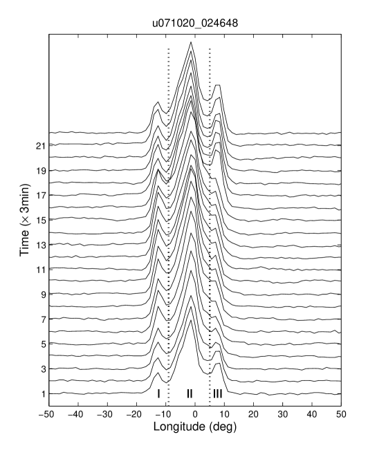
Figure 1: A sequence of pulse profiles observed in 2007 October 20 which contained both the normal and abnormal modes, each averaged over 3 minutes. The 4th to the 15th integrated profiles show switches to the abnormal mode. The dotted lines are the inner boundaries that divide the profiles into three components, I, II and III.

Two kinds of data in the total 521-hour observations from 2003 to 2009 were used in this work. The first kind consists of two long passages of quasi-continuous observations between 2004 March 12 and March 31. The observation lasted for $182$ hr in the first 8-d passage, and then $178$ hr in the second passage after an interruption of 2.3 days. They are very useful for studying the properties of moding timescales. The second kind consists of the other 90 separated observations from 2003 to 2009, which lasted for at least 0.5 hour and mostly longer than 2 hours (see Table 1). These data are used to check the long-term variability of mode switching.

Table 1: The selected 90 separated observations with the 25m telescope at UAO.

Obs. Date	MJD	$t_{\rm tot}$	Obs. Date	MJD	$t_{\rm tot}$	Obs. Date	MJD	$t_{\rm tot}$
(yymmdd)		(hr)	(yymmdd)		(hr)	(yymmdd)		(hr)
030924	52906.1	2.1	061230	54099.7	3.0	080630	54647.7	2.0
031207	52980.8	2.0	070128	54128.6	0.7	080705	54652.8	2.0
031210	52983.6	2.0	070226	54157.7	1.5	080712	54659.3	2.0
031220	52993.7	1.1	070320	54179.5	3.0	080716	54663.1	2.0
040104	53008.6	2.0	070409	54199.6	0.6	080726	54673.1	2.0
040117	53021.8	2.0	070625	54276.3	2.2	080727	54674.3	2.0
040207	53042.4	2.0	070714	54295.3	2.4	080807	54685.9	1.9
040216	53051.6	1.8	071020	54393.1	3.0	080815	54693.0	2.0
040522	53147.4	1.7	071216	54450.8	3.0	080827	54705.1	2.0
040523	53148.3	1.2	071217	54451.8	3.0	080908	54717.7	2.0
051209	53713.7	0.9	071228	54462.3	0.6	080920	54729.2	2.0
051220	53724.0	1.0	071228	54462.3	2.0	080927	54736.6	2.0
051220	53724.4	1.0	080107	54472.4	2.0	081007	54746.0	2.0
051225	53729.5	1.0	080116	54481.7	2.0	081010	54749.7	2.0
060116	53751.7	2.0	080128	54493.6	2.0	081023	54762.6	2.0
060126	53761.6	3.0	080130	54495.0	2.0	081102	54772.5	0.9
060209	53775.6	1.4	080222	54518.4	2.0	081102	54772.6	2.0
060209	53775.7	1.5	080302	54527.2	2.0	081115	54785.1	2.0
060221	53787.2	1.0	080304	54529.7	2.0	081130	54800.7	2.0
060310	53804.2	2.0	080330	54555.2	1.7	081208	54808.7	2.0
060314	53808.4	0.8	080408	54564.5	2.0	081219	54819.2	2.0
060331	53825.9	1.6	080409	54565.4	2.0	081229	54829.8	2.0
060402	53827.4	1.0	080416	54572.0	2.0	081230	54830.9	1.6
060412	53837.2	1.0	080427	54583.5	2.0	090106	54837.9	1.8
060424	53849.1	2.7	080510	54596.4	2.0	090120	54851.1	2.0
061126	54065.8	0.7	080519	54605.4	2.0	090212	54874.3	2.0
061207	54076.8	0.7	080614	54631.3	2.0	090219	54881.4	2.0
061209	54078.8	0.7	080615	54632.4	2.0	090303	54893.4	1.5
061221	54090.8	0.7	080617	54634.3	1.8	090318	54908.6	2.0
061230	54099.6	1.1	080630	54647.1	1.9	090405	54926.5	2.0

$t_{\rm tot}$ is the total time of each observation.

To fill the gaps between the sub-windows of quasi-continuous observations in 2004 (see more details in §3.2), we applied the monitoring data at 610 MHz for PSR B0329+54 obtained with the 15 m telescope at JBO. The observations were made 3 to 5 times nearly everyday since 1990. Each of them lasted for about 10 minutes and yielded an integrated profile. Only the integrated profiles are available now. These observations are helpful to verify the modes at 1540 MHz under the scenario that mode switches happen simultaneously at different frequencies, which is supported by previous observations (Bartel et al. 1982). Six gaps in the UAO data are filled by the JBO data, as shown by the circles in Figs.2 and 3.

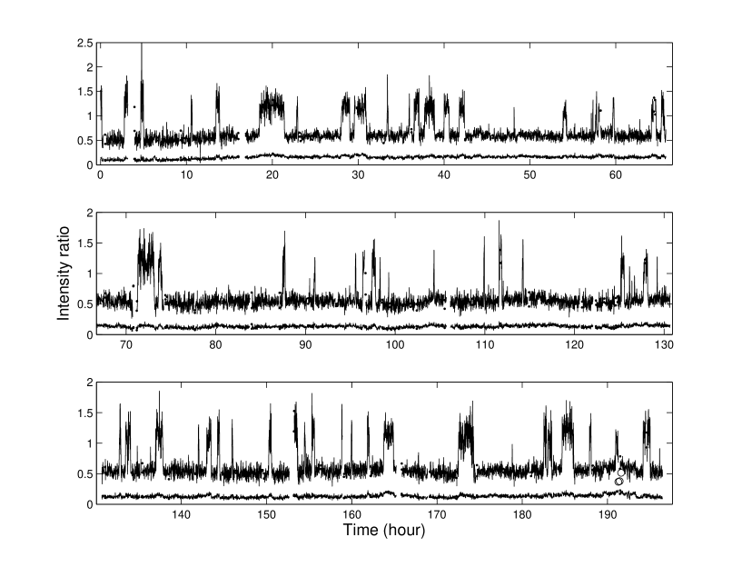
Figure 2: Time sequence of $R$ and $R^{\prime}$ for the first 8-day quasi-continuous observation from 2004 March 12 to March 20. The upper curve in each panel is the intensity ratio $R$ between the components I and III, the lower curve is the ratio $R^{\prime}$ between the components 1 and II. The integration time for individual profiles is 1 minute. The circles, of which the values are the ratios of $R$ at 610 MHz, represent the gap which are filled by the data of Jodrell Bank Observatory.

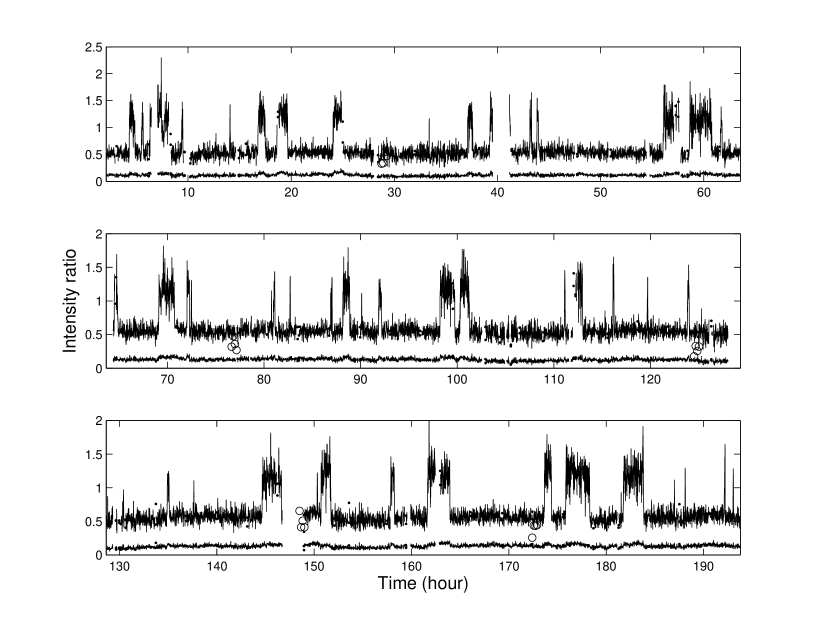
Figure 3: The time sequence of $R$ and $R^{\prime}$ for the second 8-day quasi-continuous observation from 2004 March 23 to March 31.

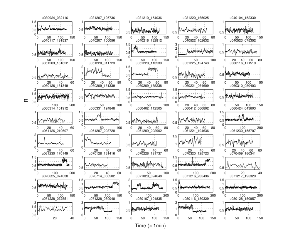
Figure 4: Time sequences of the ratio $R$ for the former 45 observations in Table 1. The integration time for the individual profiles is 1 minute.

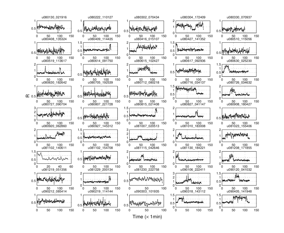
Figure 5: Time sequences of the ratio $R$ for the latter 45 observations in Table 1. The integration time for the individual profiles is 1 minute.

3 Data reduction and Results

At 1.5 GHz, the average pulse profile of PSR B0329+54 consists of three apparent components (Fig. 1). Being classified as the triple or possibly the multiple type (Rankin 1993), the integrated profiles of this pulsar can be separated into five (Kramer et al. 1994) or even nine components (Gangadhara & Gupta 2001) by using Gaussian decomposition techniques. Whereas in this paper, we separate the profiles into three components, hereafter called component I (the leading), II (the central) and III (the trailing), by a direct and simple way described as follows. Note that the most prominent feature of the mode changing is the variation of relative intensity between the leading and trailing components, even with our simple reduction, the ratio $R=I_{\rm I}/I_{\rm III}$ is still a good indicator to distinguish different modes, where $I_{\rm I}$ and $I_{\rm III}$ represent the integrated intensity of components I and III, respectively. The relative intensity between components I and II, defined as $R^{\prime}=I_{\rm I}/I_{\rm II}$, is also calculated, although it is not so sensitive as $R$ in identifying different modes.

In order to calculate $R$ and $R^{\prime}$, the phase intervals of components are determined by the following three steps. Firstly, a reference profile with high signal to noise ratio was produced by summing all the profiles of one mode in an observation. Secondly, for simplicity, the outer boundaries of components I and III are confined at 10% level of the leading and trailing pulse peaks of the reference profile, while the inner boundaries are defined as the points of minimal intensity between components I (or III) and II. Thirdly, the target profiles averaged over a few minutes are correlated and aligned with the reference profile in the same observation. In order to reduce the uncertainty in determining the inner boundaries, the target and reference profiles are smoothed by cubic interpolation in a higher resolution of 256$\times$5 sampling points per period. The examples of reference profiles and phase boundaries are shown in Fig 6, which are integrated over 25 min. and 15 min. for the normal and abnormal modes, respectively.

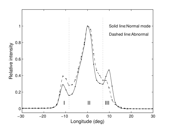
Figure 6: The average pulse profiles of PSR B0329+54 for the normal (solid) and abnormal modes (dashed), which are integrated over more than 2000 pulse periods respectively. The dots are parts of the 256 sampling points in and near the pulse window. The solid and dashed curves represent the smoothed profiles by cubic interpolation in a higher sampling resolution of $256\times$5.

Most previous work on mode switching of PSR B0329+54 used about 3 min (about 250 periods) as the integration time to suppress the pulse-to-pulse fluctuations (Lyne 1971, Bartel et al. 1982, Liu et al. 2005). Moreover, some authors suggested that more stringently the profile stability timescales in the normal and abnormal modes at 1.4 GHz would be $\sim$6  min and $\sim$36  min respectively (Helfand 1975). But in this work, since a short integration time is necessary to resolve short moding timescales, we use an integration time of 1 minute, under which the modes can be well distinguished, as demonstrated below.

3.1 Identification of two modes

The normal and abnormal modes are easily distinguished according to their evident difference in $R$. The results are presented in Figs. 2 and 3 for the two 8-day quasi-continuous observations in March 2004, and in Figs. 4 and 5 for the remaining 90 separate observations. It shows abrupt and simultaneous changes of $R$ and $R^{\prime}$ during mode switches, despite that the difference of $R^{\prime}$ between modes is less significant. In general, the ranges of $R$ are between (0.35-0.8) for the normal mode and (0.7-1.8) for the abnormal mode.

The number of the modes can be determined from the statistical distribution of $R$ values. For the two apparent states separated by the abrupt changes of $R$, by using Kolmogorov-Smirnov (KS) test, we found that the distributions of their $R$ are consistent with the normal distribution, therefore confirmed the identification of two modes. The best fit values of the mean $R_{\mu}$ and the standard deviation $w$ of the normal distribution at 95% confidence level are listed in Table 2. The probability of KS-test $p$ is also shown in the table, where the subscript “1” stands for 1-minute integration. Although the probabilities is low for the abnormal mode, they all exceed the 5% criteria below which the null hypothesis that the data follow a normal distribution is rejected. A KS-test for $R$ obtained with 3-minute integration time can considerably enhance the probability of the abnormal mode, as shown by $p_{3}$ in the table, giving further support to the identification of modes. More details about the histograms of the ratio $R$ with different integration time are described in the Appendix.

The $R$ distribution of abnormal mode is considerably wider than that of the normal mode, indicating that the abnormal mode is less stabler than the normal mode, which is consistent with the statement of Helfand (1975) that the timescale for the abnormal mode to get stable is longer than the normal mode.

Table 2: The best fit parameters for the normal and abnormal modes with normal distributions.

Parameters	$R_{\mu}$	$w$	$R^{\prime}_{\mu}$	$w^{\prime}$	$p_{1}$	$p_{3}$
	Two long	quasi-continuous	observations
Normal mode	$0.546\pm 0.002$	$0.082\pm 0.002$	$0.127\pm 0.001$	$0.027\pm 0.001$	0.996	0.760
Abnormal mode	$1.168\pm 0.008$	$0.182\pm 0.008$	$0.161\pm 0.001$	$0.026\pm 0.001$	0.098	0.748
	The remaining	90 observations
Normal mode	$0.582\pm 0.002$	$0.071\pm 0.002$	$0.1445\pm 0.0005$	$0.0215\pm 0.0008$	0.233	0.581
Abnormal mode	$1.176\pm 0.007$	$0.170\pm 0.007$	$0.1738\pm 0.0013$	$0.0229\pm 0.0013$	0.070	0.760

$p_{1}$ is the probability of KS-test for the $R$ distribution with an integration time of 1 min. and $p_{3}$ of 3 min.

3.2 Temporal properties

Among all the 521-hour UAO data, the total duration of the normal and abnormal modes are about 84.9% and 15.1%, respectively. In the two passages of 8-day observations, the percentage of the abnormal mode is about 83%. This is in agreement with the previous results (Bartel et al. 1982, Xilouris et al. 1995).

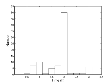
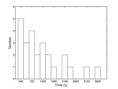
Figure 8: Left: histograms of the time duration of the 90 separated observations listed in Table 1. Right: histograms for the timescales of the complete sequences of the abnormal mode.

Totally 43 sequences of the abnormal mode are detected in the 90 separated observations, including 25 sequences of completed abnormal events. The histograms of the duration of observation windows and the timescales of the completed abnormal sequences are presented in the left and right panels of Fig. 8, respectively. It shows that the occurrence of the abnormal mode decreases at longer timescales, but the limited number of moding events and the strong selection effect of separated observation windows prevent us from determining meaningful results of timescale distribution.

In the two long quasi-continuous observations, 244 normal and 133 abnormal sequences were identified. The two observations consist of 148 sub-windows and 147 time gaps, of which the histograms are shown in the upper panels of Fig. 9. Histograms made with the UAO data are shown in the middle panels of Fig. 9, where the solid bins stand for the timescales of completed sequences, and the dashed bins for both the completed and the incompleted sequences. Compared with the normal mode, the proportion of the incompleted sequences of abnormal mode is much lower. This suggests that the abnormal mode is less affected by the selection effect of observation sub-windows, and its typical timescale is much shorter than that of the normal mode.

Since the observed timescale distribution is a convolution of intrinsic distribution and discontinuous sub-windows, it raises a question: how can we constrain the intrinsic distribution from observations? We follow two steps to make the constraint, first to suppress the selection effect by inferring the states in short gaps, and then to employ Bayesian inference to constrain the intrinsic distribution. In Bayesian inference, the timescales of the incompleted sequences tend to bias the constrained model parameters, hence it is vital to fill the gaps and increase the proportion of the completed sequences. This step is feasible, because most time gaps in the UAO data are very short, the states could be determined with the JBO data or be inferred reasonably according to the trend near the gaps.

For the six gaps that are completely or partially filled by Jodrell Bank observations, the emission states are found to be in the normal mode. For most of the other gaps less than 10 minutes, their modes are inferred to be the same as those both prior and posterior to the gaps. The probability that these assumptions are correct should be much higher than the probability that they are wrong, because only about $1/3$ of the completed abnormal sequences and $1/4$ of the completed normal sequences are shorter than 10 minutes, hence the emission happens to change its mode in such a short gap is low. Furthermore, since the above mentioned six gaps in the UAO data all appear in the tracks of normal sequences and the longest one lasts for nearly 8 minutes, the confirmation of normal mode by the JBO data gives additional support for our assumptions. The histograms for the timescales of the normal and abnormal modes after the reduction are shown in the bottom panels of Fig. 9, where the proportion of the incompleted sequences is reduced significantly, especially on long timescales, thus the selection effect is considerably suppressed.

According to the Bayes’ theorem, for any model $M$ with the parameter $\theta$, the posterior probability of $\theta$ given data $D$ is proportional to the prior probability of the parameter, $p(\theta)$, and the probability of seeing the data given $\theta$, $p(D|\theta)$, namely, $p(\theta|D)\propto p(\theta)p(D|\theta)$. It gives an estimation of the probability that the parameter happens to be valid to interpret the data. This is useful for finding the optimal value of parameter for a model by maximizing $p(\theta|D)$. However, even when the true model is unknown prior, one needs to compare the Bayesian factors of some candidate models in order to select the most likely one. The Bayesian factor $I$ is the sum of probabilities of data given all possible parameter values in the model $M$, i.e. $I=\int_{\theta_{1}}^{\theta_{2}}p(D|\theta)p(\theta){\rm d}\theta$. In the case of $N$ candidate models, if the sum of probabilities ($I$) of the other $N-1$ models is negligible compared with the total probability of all the $N$ models, i.e. $\sum\limits_{{\rm i}=2}^{N}I_{\rm i}/\sum\limits_{{\rm i}=1}^{N}I_{\rm i}<<1$, then the model $i=1$ is favored over the other models (Ghosh 2007).

We select four candidate models that may fit the data, i.e. (A) the gamma distribution with the probability density function (PDF) $p(t)=\tau^{-k}t^{k-1}{\rm e}^{-t/\tau}/\Gamma(k)$, (B) the half normal distribution with $p(t)=2\tau^{-1}{\rm e}^{-{t^{2}}/{2\tau^{2}}}/\sqrt{2\pi}$ ($t>0$), (C) the log-normal distribution with $p(t)=t^{-1}\tau^{-1}{\rm e}^{-(\ln t)^{2}/{2\tau^{2}}}/\sqrt{2\pi}$ and (D) the Pareto (power-law) distribution with $p(t)=kt^{-(k+1)}$. Model A is a two-parameter model described with the shape $k$ and the scale $\tau$, while B, C and D are one-parameter models. In a special case with $k=1$, the gamma distribution reduces to the exponential distribution. Their PDFs and statistical means are summarized in Table 3.

Lacking knowledge of the prior probability, we assume that all the prior probabilities are uniform within a parameter range $\theta_{1}\leq\theta\leq\theta_{2}$, i.e. $p(\theta)=1/(\theta_{2}-\theta_{1})$. The maximum $\theta_{2}$ is set to be large enough so that the accumulated probability at $\theta>\theta_{2}$ is negligible. In practice, we use the criterion $\int_{\theta_{2}}^{\infty}p(D|\theta){\rm d}\theta=0.001\int_{\theta_{1}}^{\infty}p(D|\theta){\rm d}\theta$ to estimate $\theta_{2}$. The second term of the Bayesian factor, i.e., the likelihood $p(D|\theta)$, is the product of the independent probabilities that the observed timescales $t_{\rm i}$ are interpreted given $\theta$. For a timescale of a completed sequence, its independent probability $p_{\rm c}(t_{\rm i}|\theta)$ is the value through substituting $\theta$ and the timescale into the PDF $p(t)$, thus the likelihood reads $p(D|\theta)=\prod\limits_{i=1}^{N_{\rm c}}p_{\rm c}(t_{\rm i}|\theta)$.

The Bayesian factors are calculated for the normal and abnormal modes with their timescale data of the completed sequences, which are denoted as $I_{\rm n}$ and $I_{\rm a}$ separately in Tab. 3. The lower limit $\theta_{1}$, specifically to say, $k_{1}$ for the Pareto and $\tau_{1}$ for the other three models, are set to be 0, while the upper limits $k_{2}$ and $\tau_{2}$ are calculated following the above criterion. As to the gamma distribution, the Bayesian factor is calculated by integrating over the scale $\tau$, hence it is a function of the shape $k$, i.e. $I(k)=\int_{\tau_{1}}^{\tau_{2}}p(D|k,\tau)p(\tau){\rm d}\tau$, as shown by the upper panels in Fig. 7. The optima and 95% confidence intervals are $k_{\rm n}=0.75^{+0.22}_{-0.17}$ for the normal mode and $k_{\rm a}=0.84^{+0.28}_{-0.22}$ for the abnormal mode. The results are summarized from rows 3 to 8 in Tab. 3.

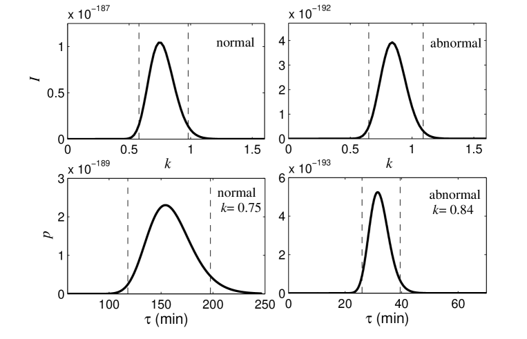
Figure 7: The Bayesian factor $I$ versus the shape parameter $k$ of the gamma distribution and the likelihood $p$ versus the time scale $\tau$ for the normal and abnormal modes. In the lower two panels, the likelihood is calculated given the optimal shape parameter $k_{\rm n}=0.75$ for the normal mode and $k_{\rm a}=0.84$ for the abnormal mode. The dashed lines denote the 95% confidence intervals of $k$ and $\tau$ around their optima.

Among the four models, the gamma distribution is favored because its Bayesian factors are higher than those of the others by more than 10 orders of magnitude. Given the optimal shape parameter $k_{\rm n}=0.75$ and $k_{\rm a}=0.84$, the scale parameter is constrained to be $\tau_{\rm n}=154^{+41}_{-36}$ minutes and $\tau_{\rm a}=31.5^{+8.0}_{-5.5}$ minutes, respectively, through maximizing the likelihood $p(D|k,\tau)$ and calculating the 95% confidence intervals (see the lower panels in Fig. 7). Then, the PDFs of the optimal distributions are $p_{\rm n}(t)=0.019t^{-0.22}{\rm e}^{-t/154}$ for the normal timescales and $p_{\rm a}(t)=0.049t^{-0.16}{\rm e}^{-t/31.5}$ for the abnormal timescales. To compare with the data, we also plot the number density functions of these two distributions in Fig. 9 (the curves in the lower panels). The functions reads ${\rm d}n/{\rm d}t=n_{0}p(t)$, where ${\rm d}n$ is the number of the moding events within the duration $t\pm{\rm d}t$, and $p(t)$ is the PDF of gamma distribution. The constant $n_{0}$ is determined by minimizing $\chi^{2}=\sum\limits_{{\rm i}=1}^{{\rm n_{b}}}(N_{\rm i}-n_{\rm i})^{2}/n_{\rm i}$, where $N_{\rm i}$ and $n_{\rm i}$ are the observed and modeled numbers of the complete sequences in the i$-$th bin, n_b is the total number of bins. Because $N_{\rm i}$ and $n_{\rm i}$ do not follow normal distributions, this estimation is an approximation to the real number density function when n${}_{\rm b}>>1$ (Press et al. 1992), and here it is only meaningful for visualization of the constrained gamma distributions and comparison with the data.

Table 3: Results of Bayesian inference for four candidate models.

models	gamma	half normal	log-normal	Pareto
PDF	$\frac{1}{\tau^{k}\Gamma(k)}t^{k-1}{\rm e}^{-t/\tau}$	$\frac{2}{\sqrt{2\pi}\tau}{\rm e}^{-\frac{t^{2}}{2\tau^{2}}}$	$\frac{1}{\sqrt{2\pi}t\tau}{\rm e}^{-\frac{(\ln t)^{2}}{2\tau^{2}}}$	$\frac{k}{t^{k+1}}$
mean	$k\tau$	$\sqrt{\frac{2}{\pi}}\tau$	${\rm e}^{\frac{\tau^{2}}{2}}$	$\frac{k}{k-1}$
		Normal mode
$\theta_{2,{\rm n}}\tablenotemark{\ast}$	216.5	199.7	5.69	0.30
$\lg I_{\rm n}$	-188.7	-204.7	-231.7	-207.9
($k_{\rm n}$, $\tau_{\rm n})$	($0.75^{+0.22}_{-0.17},154^{+41}_{-36}$)	$-$	$-$	$-$
		Abnormal mode
$\theta_{2,{\rm a}}\tablenotemark{\ast}$	45.5	53.8	3.59	0.50
$\lg I_{\rm a}$	-192.1	-205.8	-231.9	-209.9
($k_{\rm a}$, $\tau_{\rm a})$	($0.84^{+0.28}_{-0.22},31.5^{+8.0}_{-5.5}$)	$-$	$-$	$-$

^∗Stands for $k_{2}$ for the Pareto distribution and $\tau_{2}$ for the other three (in unit of minute). $\tau$ in unit of minute.

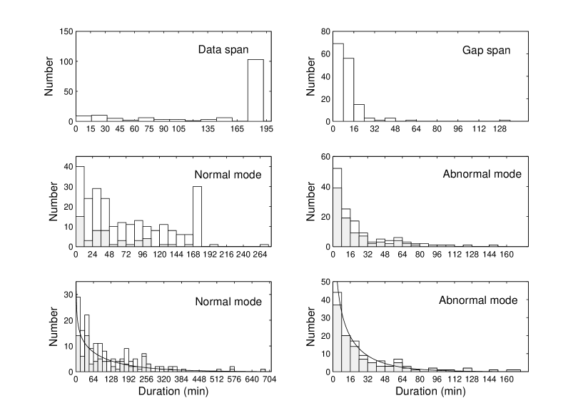
Figure 9: Upper: histograms of the time duration of the observing sub-windows from 2004 March 12 to March 31 (left) and that of the gaps between the sub-windows (right). Middle: histograms of the observed apparent timescales of the normal mode (left) and the abnormal mode (right). Lower: histograms of the corrected timescales of the normal mode (left) and the abnormal mode (right) after reduction of short gaps (see text for details). The grey bins are for the complete sequences, while the white bins are for both the complete and the incomplete sequences. The curves in the lower panels stands for the constrained optimal gamma distributions (see text for details).

3.3 Long-term modulation

For the whole UAO observations in seven years, the ratios $R$ and $R^{\prime}$ and their $1\sigma$ errors are plotted in Fig. 10 for the normal (open triangles) and abnormal (solid diamonds) modes separately. Each point stands for the averaged $R$ for a normal or a abnormal sequence longer than 25 minutes. The averaged ratio and the error are measured from a number of profiles integrated over 3 minutes in that observation.

The JBO daily data contain 6243 useful profiles over 19 years. Fig. 11 shows fluctuation of ratio $R$ when averaging the profiles over different time intervals. For larger intervals, two modes tend to be fully mixed and the ratio becomes stable. The results do not show evident long-term variation.

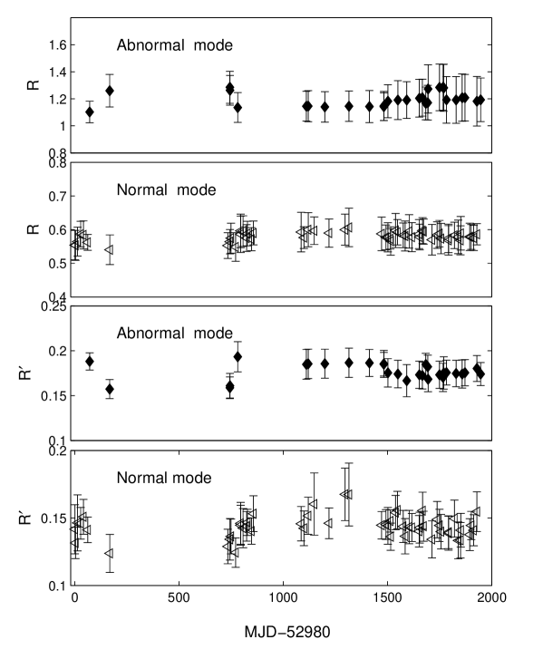
Figure 10: Time-dependent $R$ and $R^{\prime}$ for the normal and abnormal modes from 2003 to 2009 obtained with the UAO data. The open triangles and the solid diamonds correspond to the normal and abnormal modes, respectively. Only the observations in which the normal mode or the abnormal mode lasts long enough are selected to make this plot.

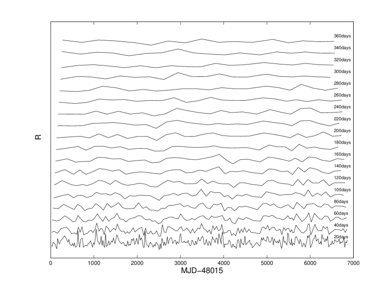
Figure 11: The long-term fluctuation of $R$ with the JBO data at 610 MHz. The numbers at right side represent the intervals in which daily profiles are summed.

4 Conclusions and discussions

PSR B0329+54 presents two modes based on the distribution of $R$ in our work. Totally 176 mode switching events were detected, among which 133 occurred during the observation in March 2004. The major difference between the normal and abnormal modes is the intensity ratio between the leading and trailing components and the length of moding timescales. In particular, the two passages of eight-day quasi-continuous observations from 2004 March 12 to March 31 provide an opportunity to constrain the intrinsic distributions of timescales for the first time. The main observational properties and concluding remarks are summarized as follows.

(1) The intensity ratios ($R$) between the leading and trailing components of average pulse profiles follow normal distributions, of which the means are 0.56 for the normal mode and 1.17 for the abnormal mode, respectively. The distribution of the abnormal mode is wider than that of the normal mode, suggesting that it is less stabler than the normal mode.

(2) The pulsar spent 84.9% of the total observation time in the normal mode, and 15.1% in the abnormal mode. The observed longest normal and abnormal pulse tracks lasted 4.4 and 2.47 hours, respectively, while they are likely as long as 11 and 2.88 hours when the mode in short gaps between observational sub-windows were carefully inferred. No periodicity was found in the quasi-continuous time sequences of mode switching in 2004.

(3) By virtue of the Bayesian inference, it is found that the gamma distribution is a better description for the intrinsic distribution of moding timescales than the other considered models, e.g. the normal, log-normal and Pareto distributions. The optimal gamma distributions have the shape parameter 0.75${}^{+0.22}_{-0.17}$ and the scale parameter $154^{+41}_{-36}$ minutes for the normal mode, and $0.84^{+0.28}_{-0.22}$ and $31.5^{+8.0}_{-5.5}$ minutes for the abnormal mode.

(4) In the UAO 7-year data and the JBO 19-year data, no prominent long-term modulation on mode switching was observed.

Mode switching was suggested by many authors to be the phenomenon that pulsars switches between different magnetospheric states, likely to be caused by changes of magnetospheric particle current flow (e.g. Lyne 1971, Bartel et al. 1982). Recently, Lyne et al. (2010) found that the changes in timing noise are directly related to the changes in pulse shape for six pulsars. The profiles of all the six pulsars switches between two states in moding timescales from a few days to hundreds of days. The change of pulsar spin-down rate $\dot{\nu}$ is highly correlated or anti-correlated with the change of pulse profiles. This discovery, together with the correlation between spin-down rate and “on” and “off” modes found in the intermittent pulsar B1931+24, give clear evidence for the mechanism of changes of magnetospheric current flow. When the current is enhanced, pulsars spin down faster and pulse profiles stay in one mode, then they switches to another mode and spin down slower when current is reduced. As to PSR B0329+54, unfortunately, the moding timescales are too short to derive useful $\dot{\nu}$. In a long period of time needed to obtain the spin-down rate, two modes are mixed in a proportion depending on the real integration time and tends to be normal/abnormal=85%/15% when the integration time is longer enough (see Fig. 11 as examples). Using the archived data, we did not find any correlation between the timing and the moding for B0329+54.

The underlying physical reason for the change of magnetosphere state is not clear yet. Two possible mechanisms were proposed in literature. Zhang et al. (1997) suggested that the alteration of the temperature of pulsar surface could trigger different sparking modes in the inner vacuum gap, thus results in mode switching phenomenon. It was found that the gap sparking could be dominated by magnetic absorption of the gamma-ray photons generated via curvature radiation or inverse Compton scattering (ICS). In the ICS process, the gamma-rays generated via resonant scattering of the thermal X-ray photons from the pulsar surface and non-resonant scattering of the thermal peak X-ray photons have priority in breaking down the vacuum gap. These three modes, i.e. the curvature mode, the resonant ICS mode and the thermal-peak ICS mode are separated by two critical temperatures. Thus when the temperature fluctuates around a critical value, the sparking mode will change suddenly. Although it was demonstrated that the key parameter of the ICS modes, i.e. the mean free path of the electron is a function of the temperature, the process how different sparking modes can lead to different emission modes has not been investigated. Future simultaneous and continuous radio and X-ray monitoring will be helpful to test this mechanism by searching for correlation between the emission mode and the pulsar surface temperature.

Timokhin (2010) proposed that it could be switches in the magnetosphere geometry or/and redistribution of the currents flowing in the magnetosphere that change the pulsar emission beam and its orientation with respect to the line of sight and hence lead to the mode switching phenomenon. The possible mechanism, as the author speculated, might be that the combination of current density distributions and different sizes of the co-rotating zone could result in a set of meta-stable magnetosphere configurations, which represent local minima of the total energy of magnetosphere. Some meta-stable configurations may be a kind of strange attractors, where the magnetospheric system spends a period of time in one state and then suddenly changes to another one.

Mode switching is likely to be related to stochastic dynamic processes in pulsar magnetosphere. Then, the statistical property of moding timescales is very useful to understand the physics of the non-linear system. For PSR B0329+54, as our observation shows, the waiting time until another state takes place is not quasi-periodical, but follows the gamma distributions. Further dynamic models based on, e.g. the cascade process in gaps, or the global current flow in the magnetosphere, or some sorts of instabilities, need to reproduce the observed distribution. PSR B0329+54 is yet the only pulsar with known distributions of the moding timescale. Long-term continuous monitoring for other mode-changing pulsars will find out if they have the same or various kinds of distribution, therefore will provide more constraints on the underlying physics.

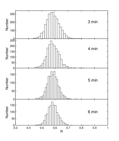
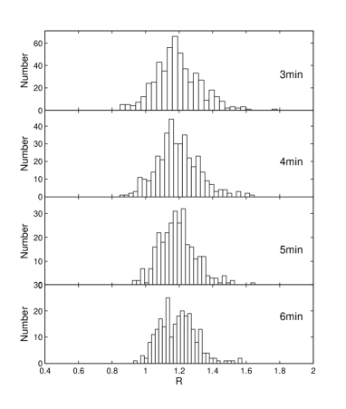
Figure 12: $R$ distributions versus different integration times for the normal (left) and abnormal (right) modes by using the data of the 90 separated observations.

References

- Bac (1970) Backer, D.C.,1970, Nature, 228, 1297
- Bar (1978) Bartel, N.,Sieber, W., Wielebinski, R. 1978, Astron. Astrophys., 68, 361
- Bar (1982) Bartel, N., Morris, D., Sieber,W. et al., 1982, ApJ, 258,776
- Gan (2001) Gangadhara, R. T. & Gupta, Y., 2001, ApJ, 555, 31
- Gho (1982) Ghosh, J. K., 2007, ASPC, 371, 206
- Hel (1975) Helfand, D.J., Manchester, R.N., Taylor, J.H., 1975, ApJ, 198, 661
- Hes (1973) Hesse, K.H, 1973, A&A, 27, 33
- Kra (1994) Kramer, M., 1994, Astron. Astrophys. Suppl. Ser. 107, 527
- Kra (1997) Kramer, M., Xilouris, K. M., Jessner, A., et al.,1996, A&A, 306, 867
- Kra (1997) Kramer, M., Jessner, A., Doroshenko, O. et al.,1997, ApJ, 488, 364
- Kra (2003) Kramer, M., Karastergiou A., Gupta Y. et al., 2003, A&A, 407, 655
- Lyn (1971) Lyne, A. G., 1971, MNRAS, 153, 337
- Lyn (1988) Lyne, A. G., Manchester, R. N., 1988, MNRAS, 234, 477
- Lyn (2010) Lyne, A. G., 2010, Sci, 329, 408
- pre (1992) Press, W.H., Teukolsky, S.A., Vetterling W.T. et al., 1992, Numerical Recipes, second edition, Cambridge University Press Syndicate, 614-622
- Ran (1983) Rankin, J. M., 1983, ApJ, 274, 359
- Ran (1986) Rankin, J. M., 1986, ApJ, 301, 901
- Ran (1998) Rankin, J. M., 1988, ApJ, 324, 1048
- Ran (1998) Rankin, J. M., 1993, ApJS, 85, 145
- Sul (1998) Suleimanova, S.A., Izvekova V.A., Astrophys Astr., 1998, 19, 1
- Sul (2002) Suleimanova, S.A., Pugachev,V.D., 2002, Astronomy Reports, Volume 46, Issue 1, January 2002,pp. 34-48
- Tim (2010) Timokhin, A. N., 2010, MNRAS, 408, 41
- Wan (2001) Wang, N., Manchester, R. N., Zhang, J. et al. 2001, MNRAS, 328, 855
- Wan (2008) Wang, N., Yan,Z., Manchester, R. N. et al. 2008, MNRAS, 385, 1393
- Wri (1981) Wright, G. A., Fowler L. A., 1981, Astron. Astrophys., 101, 356
- xil (1995) Xilouris, K. M., Seiradakis, J. H., Gil, J., et al., 1995, A&A, 293,153
- zha (1997) Zhang, B., Qiao, G. J., Lin, W. P. et al., 1997, ApJ, 478, 313