Modified exponential I(U) dependence and optical efficiency of AlGaAs SCH lasers in computer modeling with Synopsys TCAD.

Abstract

Optical and electrical characteristics of AlGaAs lasers with separate confinement heterostructures are modeled by using Synopsys’s Sentaurus TCAD, and open source software. We propose a modified exponential $I-V$ dependence to describe electrical properties. A simple analytical, phenomenological model is found to describe optical efficiency, $\eta$, with a high accuracy, by using two parameters only. A link is shown between differential electrical resistivity $r=dU/dI$ just above the lasing offset voltage, and the functional $\eta(U)$ dependence.

1 Introduction

Alferov [1], et al., proposed creating semiconductor-based lasers comprising the use of a geometrically-narrow active recombination region where photon generation occurs, with waveguides around improving the gain to loss ratio (separate confinement heterostructures; SCH). That idea dominated largely the field of optoelectronics development in the past years. Due to the relative simplicity and perfection of technology, solid solutions of $Al_{x}Ga_{1-x}As$ are commonly used as wide-gap semiconductors in SCH lasers.

Reaching the threshold current density of these lasers less than $1kA/cm^{2}$ at room temperature has opened up prospects for their practical application and served as a turning point in their production. Now, they are mostly used for pumping solid state $Nd:YAG$ lasers, either for high-power metallurgical processes or, already, in first field experiments as a highly directional source of energy in weapons interceptors. Further progress in that direction is associated with optimizing the design of laser diodes and, in particular, in improving their optical efficiency as well finding methods of removing excess heating released.

In our earlier works we first were able to find agreement between our calculations of quantum well energy states and the lasing wavelength observed experimentally [2]. Next [3], we have shown how to considerably improve their electrical and optical parameters by finding the most optimal QW width and waveguides widths, and type and level of doping [4]. We compared computed properties with these of lasers produced by Polyus research institute in Moscow [5], [6]. By changing the waveguide profile through introducing a gradual change of Al concentration, as well variable doping profiles, we were able to decrease significantly the lasing threshold current, increase the slope of optical power versus current, and increase optical efficiency.

We have shown also [7] that the lasing action may not occur at certain widths or depths of Quantum Well (QW), and the threshold current as a function of these parameters may have discontinuities that occur when the most upper quantum well energy values are very close to either conduction band or valence band energy offsets. These effects are more pronounced at low temperatures, and may be observed also, at certain conditions, in temperature dependence of lasing threshold current as well.

One of the fundamental laser characteristics is their optical efficiency, $\eta$, the ratio of optical power generated, $L$, to electrical power supplied, $\eta=L/(U\cdot I)$, as well dependence of $\eta$ on current or voltage. We propose here a simple analytical, phenomenological model for description of $I-V$ characteristics near and above lasing offset voltage $U_{0}$, and we show that that model may be used for description of $\eta(U)$ with a high accuracy. At the same time we obtain a link between differential electrical resistivity $r=dU/dI$ just above $U_{0}$, with the functional $\eta(U)$ dependence, where $r$ is also an important experimental characteristic of a laser device.

For simulations, we use Sentaurus TCAD from Synopsys [8], which is an advanced commercial computational environment, a collection of tools for performing modeling of electronic devices.

2 Lasers structure and calibration of modeling.

We model a laser with $1000\mu m$ cavity length and $100\mu m$ width, with doping/Al-content as described in Table 1.

Synopsys’s Sentaurus TCAD is a flexible set of tools used for modeling a broad range of technological and physical processes in the world of microelectronics phenomena. It can be run on Windows and Linux OS. Linux, once mastered, offers more ways of an efficient solving of problems by providing a large set of open source tools and ergonomic environment for their use, making it our preferred operating system. We find it convenient, for instance, to use Perl scripting language for control of batch processing and changing parameters of calculations as well for manipulation on text data files, and Tcl for manipulating (extracting) spacial data from binary $TDR$ files. A detailed description, with examples of scripts, is available on our laboratory web site.

The results for $I_{th}$ and $S=dL/dI$, in this paper, are all shown normalized by $I_{th}^{0}$ and $S_{0}$, respectively, which are the values of $I_{th}$ and $S$ computed for the reference laser described in Table 1.

We neglect here the effect of contact resistance, $R_{x}$, by not including buffer and substrate layers and contacts into calculations (compare with structure described in Table 1). An estimate, based on geometric dimensions of substrate layers and their microscopic parameters (doping concentration, carrier mobility) gives us a value of $R_{x}$ of the order of $13m\Omega$. At lasing threshold current of $0.1A$, that small resistance will cause a difference between computed by us lasing offset voltage $U_{0}$ and that measured one by about $1mV$ only. We still will however have a noticeable contribution from $R_{x}$ to differential resistance $dU/dI$.

3 Methods of data analysis.

3.1 Threshold current and $L(I)$ dependence.

The most accurate way of finding $I_{th}$ is by extrapolating the linear part of $L(I)$ to $L=0$ just after the current larger than $I_{th}$. We used a set of gnuplot and perl scripts for that that could be run semi-automatically, very effectively, on a large collection of datasets. One should only take care that the data range for fiting is properly chosen, since $L(I)$ is a linear function in a certain range of $I$ values only. The choice of that range may affect accuracy of data analysis.

3.2 $U_{0}$ from fiting $U(I)$ dependence

An exponential $U(I)$ dependence is found to work well at voltages which are well below the lasing offset voltage $U_{0}$. Near the lasing threshold, we observe a strong departure from that dependence, and, in particular, for many data curves a clear kink in $U(I)$ is observed at $U_{0}$. We find that a modified exponential dependence describes the data very well:

$$\begin{array}[]{ll}I(U)=I_{th}\cdot exp(A\cdot(U-U_{0})+B\cdot(U-U_{0})^{2}),\leavevmode\nobreak\ \leavevmode\nobreak\ \leavevmode\nobreak\ for\leavevmode\nobreak\ U<U_{0}\\ I(U)=I_{th}\cdot exp(C\cdot(U-U_{0})+D\cdot(U-U_{0})^{2}),\leavevmode\nobreak\ \leavevmode\nobreak\ \leavevmode\nobreak\ for\leavevmode\nobreak\ U>U_{0}\end{array}$$ (1)

where $I_{th}$, $U_{0}$, as well $A$, $B$, $C$, and $D$ are certain fiting parameters. Equation 1 offers a convenient interpretation of physical meaning of it’s parameters $I_{th}$ and $U_{0}$: $I(U_{0})=I_{th}$.

3.3 Differential resistance

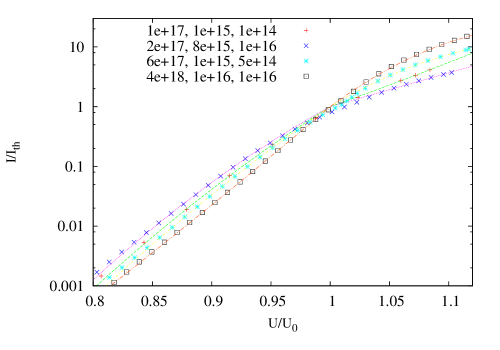
Figure 1: Examples of typical $I-V$ characteristics for a few combination (as described in the Figure) of doping concentrations (n- and p-emitters concentration first, followed by waveguides and active region concentrations). We show the narrow region near the lasing threshold, only. The curves are computed by using fiting parameters ($I_{th},A,B,C,D,U_{0}$) of equation 1, and after that voltage and current are normalized by $U_{0}$ and $I_{th}$, respectively.

The above function (Eq. 1) is continuous at $U_{0}$, as it obviously should, but it’s derivative is usually not. Figure 1 shows a few typical examples of $I(U)$ datasets. The lines were computed analytically by using Eq. 1, after finding all parameters with the least-squares method.

Since (1) may have a discontinuous derivative, using it to find out differential resistance at $U_{0}$ is ambiguous. From Eq. (1), at $U=U_{0}$, we will have $dU/dI=\frac{1}{I_{th}\cdot A}$ on the side $U<U_{0}$ and $dU/dI=\frac{1}{I_{th}\cdot C}$ on the side $U>U_{0}$. Hence, the parameter $C$ may be interpreted in terms of differential resistivity just above $U_{0}$:

$$\begin{array}[]{ll}r=\frac{1}{C\cdot I_{th}}\end{array}$$ (2)

We find from data analysis, for instance for the third dataset in Figure 1, that $dU/dI\approx 50m\Omega$, which, together with estimated contact resistance $R_{x}=13m\Omega$ gives good qualitative agreement with the differential resistance expected for real lasers, where it is in the range of about $50-80m\Omega$ ([5] and [6]).

3.4 Doping dependencies

Figure 2 shows the dependence of parameter $D$ in Eq. 1 on n-, and p-emitters doping concentration, for a very broad range of doping concentrations in other regions (this is "N-N" type of doping; see description of Table 1). Due to large scatter of the parameters obtained by the least-squares fiting, we do not distinguish between datapoints that were obtained for various doping concentrations in waveguides or in active region: the dominant factor on values of $C$ or $D$ parameters is doping concentration in emitter regions.

We observe also that a correlation exists between values of $C$ and $D$ parameters, as illustrated in Figure 3. The line in Figure 3 was obtained by using the least-squares fiting method to all the data points displayed there, with the following simple function:

$$\begin{array}[]{ll}D=-40.073+8.6\cdot 10^{-5}\cdot(41.4-C)^{3.75}\end{array}$$ (3)

It is convenient to rewrite Equation 1 in dimensionless variables. In case of $U>U_{0}$ we have then:

$$\begin{array}[]{ll}i(u)=exp\left(\frac{1}{\alpha}\cdot(u-1)\cdot\left[1+\beta\cdot U_{0}^{2}\cdot(u-1)\right]\right),\end{array}$$ (4)

where we defined: $i(u)=I(U)/I_{th}$ and $u=U/U_{0}$, $\alpha=r\cdot I_{th}/U_{0}$, $\beta=U_{0}\cdot D/C$, and we used also Eq. 2.

Let us estimate the range of reasonable values of $\beta$ parameter.

The function 3 would give the ratio $D/C\rightarrow+\infty$ for $C$ decreasing to $0$ (which corresponds to decreasing doping concentration in emitter regions to $0$). That function will pass through $0$ at values of $C\approx 8.9$, which corresponds to doping in emitters of around $2\cdot 10^{17}cm^{-3}$, will have minimum of value $\approx-1.59$ at concentrations corresponding to $\approx 2\cdot 10^{18}cm^{-3}$, and will increase to $-1$ at larger doping concentrations. The practical range of interest in our case is not at the lowest doping concentrations in emitters, since than other laser parameters deteriorate. We are left with $D/C$ values that are important to us in the range between $\approx-1.6$ and $0$.

Hence, the corresponding range of $\beta$ values that is of our interest is between $\approx-1$ and $0$.

4 Optical efficiency

4.1 A simplified approach

It is tempting to try a simplified version of 4, when the expression under exponent is $<<1$. We have in that case the following approximation on optical efficiency:

$$\begin{array}[]{ll}\eta(u)=\frac{S}{U_{0}\cdot u}\cdot\frac{(u-1)+\beta\cdot(u-1)^{2}}{\alpha+\left[(u-1)+\beta\cdot(u-1)^{2}\right]}\end{array}$$ (5)

Figure 4 shows a few example curves computed with Equation 5. The accuracy of these results, if compared with real data (not shown on that figure), appears to be far from desired; Eq. 5 may be treated as a very rough approximation only.

4.2 Exact result

Let us use however the full version of Equation 1 (for $U>U_{0}$), for computing optical efficiency. We have then:

$$\begin{array}[]{ll}\eta(u)=\frac{S}{U_{0}}\cdot\frac{i(u)-1}{u\cdot i(u)},\end{array}$$ (6)

where $i(u)$ is given by Eq. 4.

Figure 5 shows that an excellent agreement is obtained when these analytical formulas are used for approximating optical efficiency directly computed from modeling data. The parameters used in fiting the data are shown in Figure 6. As seen on this figure, the value of $\beta$ for some datapoints is lower than $-1$. This should not be considered contradictory to our estimate of the range of possible values of $\beta$: our calculations of $\eta$ do not take into account the nonlinearity of $L(I)$ dependence, which may be large, especially for low doping concentrations in emitters, and that will effectively cause decrease of $\beta$ value. We see also that the parameter $\alpha$ is too small (i.e. $(u-1)/\alpha$ is too large) in realistic cases to allow using the simplified Equation 5.

Table 1: Structure of AlGaAs SCH laser layers used in computer modeling. Values of doping concentrations listed in rows 4-6 of this table are approximate only. In this paper we make reference to two kinds of doping concentrations in these regions, that we name by "N-N" and "N-P". "N-N" means that in two waveguides there is the same N-type doping concentration with doping type in active region of n-type as well. "N-P" means" that one waveguide is of n-type doping and the other one of p-type doping. Active region has then n-type doping. The "real" lasers have N-N type of doping, however, setting "N-P" type of doping in computer modeling leads to a significant improvement of device characteristics [4].

No	Layer	Composition	Doping [$cm^{-3}$]	Thickness [$\mu m$]
1	n-substrate	n-GaAs (100)	$2\cdot 10^{18}$	350
2	n-buffer	n-GaAs	$1\cdot 10^{18}$	0.4
3	n-emitter	$Al_{0.5}Ga_{0.5}As$	$1\cdot 10^{18}$	1.6
4	waveguide	$Al_{0.33}Ga_{0.67}As$	none ($n\approx 10^{15}$)	0.2
5	active region (QW)	$Al_{0.08}Ga_{0.92}As$	none ($n\approx 10^{15}$)	0.012
6	waveguide	$Al_{0.33}Ga_{0.67}As$	none ($n\approx 10^{15}$)	0.2
7	p-emitter	$Al_{0.5}Ga_{0.5}As$	$1\cdot 10^{18}$	1.6
8	contact layer	p-GaAs	$4\cdot 10^{19}$	0.5

Figure 2: Dependence of $D$ on n-, and p-emitters doping concentration, for a broad range of doping concentrations in other regions: n-type concentration in active region changes between $10^{14}$ and $10^{16}cm^{-3}$, while n-type concentration in waveguide regions between $10^{15}$ and $10^{16}cm^{-3}$.

Figure 3: Correlation between parameters $D$ and $C$ for a broad range of doping concentrations in all regions: n-type concentration in active region changes between $10^{14}$ and $10^{16}cm^{-3}$, n-type concentration in waveguide regions is between $10^{15}$ and $10^{16}cm^{-3}$, and in emitter regions it changes between $10^{17}$ and $2.5\cdot 10^{18}cm^{-3}$. The line is described in the text.

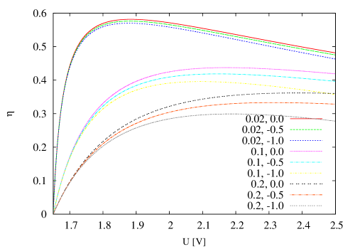
Figure 4: Optical efficiency as a function of voltage, computed by using Equation 5, for a few values of parameters $\alpha$ and $\beta$, as shown in the Figure. It has been assumed that $S=1.25W/A$ and $U_{0}=1.65V$.

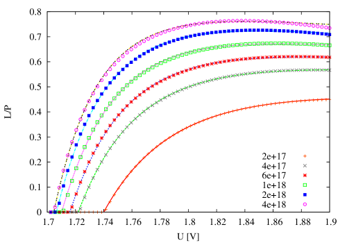
Figure 5: The lines show optical efficiency computed with equations 6 and 4, while symbols show optical efficiency directly obtained from modeling data. The results are for "N-P" type of doping structure (different type of doping for both waveguides), for doping concentration in waveguides of $1\cdot 10^{15}cm^{-3}$, in active region $5\cdot 10^{14}cm^{-3}$, and in emitter regions as shown in the Figure.

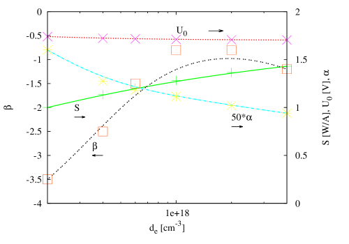
Figure 6: Parameters $S$, $U_{0}$, $\alpha$ and $\beta$ as a function of doping concentration in emitters, that were used to draw curves in Figure 5. The lines are to guide the eyes, only.

5 Summary

Computer simulations using Sentaurus TCAD from Synopsys were used for performing modeling of electrical and optical characteristics of SCH lasers based on AlGaAs.

A modified exponential $I-V$ dependence (Equations 1 and 4) is proposed to describe electrical properties.

That simple analytical, phenomenological model is found to describe one of the most fundametal laser characteristics, optical efficiency, $\eta(U)$, with a high accuracy, by using two parameters only (except of $S=dL/dI$, $I_{th}$, and $U_{0}$). At the same time we obtain a link between differential electrical resistivity $r=dU/dI$ just above lasing offset voltage, with the functional $\eta(U)$ dependence.

The proposed model is useful for both, analysis of computer modeling results as well experimental data on real devices.

6 Acknowledgements

This research was carried out under the Federal Program "Research and scientific-pedagogical cadres of Innovative Russia" (GC number P2514). The authors are indebted for valuable comments and discussions to A. A. Marmalyuk of Research Institute "Polyus" in Moscow.

References

- [1] Zh. I. Alferov, The double heterostructure concept and its applications in physics, electronics, and technology, Rev. Mod. Phys. V.73. No.3. P.767-782 (2001).
- [2] S. I. Matyukhin, Z. Koziol, and S. N. Romashyn, The radiative characteristics of quantum-well active region of AlGaAs lasers with separate-confinement heterostructure (SCH), arXiv:1010.0432v1 [cond-mat.mtrl-sci] (2010)
- [3] Z. Koziol, S. I. Matyukhin, Waveguide profiling of AlGaAs lasers with separate confinement heterostructures (SCH) for optimal optical and electrical characteristics, by using Synopsys’s TCAD modeling, unpublished, (2011).
- [4] Z. Koziol, S. I. Matyukhin, and S. N. Romashyn, Doping effects in AlGaAs lasers with separate confinement heterostructures (SCH). Modeling optical and electrical characteristics with Sentaurus TCAD. arXiv:1106.2501v1 [physics.comp-ph] (2011)
- [5] A. Yu. Andreev, S. A. Zorina, A. Yu. Leshko, A. V. Lyutetskiy, A. A. Marmalyuk, A. V. Murashova, T. A. Nalet, A. A. Padalitsa, N. A. Pikhtin, D. R. Sabitov, V. A. Simakov, S. O. Slipchenko, K. Yu. Telegin, V. V. Shamakhov, I. S. Tarasov, High power lasers ( = 808 nm) based on separate confinement AlGaAs/GaAs heterostructures, Semiconductors, 43(4), 543-547 (2009).
- [6] A. V. Andreev, A. Y. Leshko, A. V. Lyutetskiy,A. A. Marmalyuk, T. A. Nalyot, A. A. Padalitsa, N. A. Pikhtin, D. R. Sabitov, V. A. Simakov, S. O. Slipchenko, M. A. Khomylev, I. S. Tarasov, High power laser diodes ( = 808 – 850 nm) based on asymmetric separate confinement heterostructure, Semiconductors, 40(5), 628-632 (2006).
- [7] Z. Koziol, S. I. Matyukhin, and S. N. Romashyn, Non-monotonic Characteristics of SCH Lasers due to Discrete Nature of Energy Levels in QW, accepted for presentation at Nano and Giga Challenges in Electronics, Photonics and Renewable Energy Symposium and Summer School, Moscow - Zelenograd, Russia, September 12-16, (2011).
- [8] Synopsys, Sentaurus Device User Guide, www.synopsys.com, (2010)