Random walks in small-world exponential treelike networks

Abstract

In this paper, we investigate random walks in a family of small-world trees having an exponential degree distribution. First, we address a trapping problem, that is, a particular case of random walks with an immobile trap located at the initial node. We obtain the exact mean trapping time defined as the average of first-passage time (FPT) from all nodes to the trap, which scales linearly with the network order $N$ in large networks. Then, we determine analytically the mean sending time, which is the mean of the FPTs from the initial node to all other nodes, and show that it grows with $N$ in the order of $N\ln N$. After that, we compute the precise global mean first-passage time among all pairs of nodes and find that it also varies in the order of $N\ln N$ in the large limit of $N$. After obtaining the relevant quantities, we compare them with each other and related our results to the efficiency for information transmission by regarding the walker as an information messenger. Finally, we compare our results with those previously reported for other trees with different structural properties (e.g., degree distribution), such as the standard fractal trees and the scale-free small-world trees, and show that the shortest path between a pair of nodes in a tree is responsible for the scaling of FPT between the two nodes.

1 Introduction

As a powerful mathematical tool that can describe a large number of real natural and manmade systems, complex networks have received considerable interest from a wide range of scientific communities recently [1, 2, 3]. During the last decade, main endeavors were devoted to understanding the structural features and dynamics of various networks [4]. In particular, treelike networks have attracted renewed attention, because the so-called border tree motifs are present in numerous real-life systems and play a significant role [5, 6]. The absence of loops in a treelike network has a drastic influence on diverse dynamic processes running on the network, e.g., the voter model [7] and naming game [8].

Among a plethora of dynamics, random walks in trees have received increasing attention in recent years, since the problem is related to a wide range of research fields, such as physics [9], biology [10], and cognitive science [11]. One of the most important quantities of random walks is the first-passage time (FPT) [12] defined as the expected time for a walker starting from a source point to first arrive at a target node [13, 14], which encodes much information about random-walk dynamics. Thus far, random walks in trees with different structures have been intensively studied, including the standard fractal trees (e.g., the $T-$fractal [15, 16, 17, 18, 19] and the Vicsek fractal [20, 21]) and scale-free trees [22, 23, 24]. These works uncovered how the mean first-passage time (MFPT), i.e., the average of FPTs between some given pairs of nodes, scales with the network size (number of nodes), and was thus helpful for understanding the impact of structural properties on the behavior of MFPT. For example, it was shown that the MFPTs between two nodes in different trees behave different. But the main reason for the difference remains not well understood. On the other hand, in contrast to the scale-free behavior [25], some real networks display an exponential distribution as well [26]. Relevant work on random walks on such networks is much less. Particularly, what is the main factor affecting the speed of diffusion in general trees is still not well understood. A goal of this work is to answer this question, at least partially.

In this paper, we study a simple random walk [27] on a family of deterministically growing small-world trees exhibiting an exponential form of degree distribution [28]. We first address a trapping problem, which is a particular random walk with a single trap positioned at the initially created node of the networks. We derive analytically the mean tapping time (MTT) defined as the average of the FPTs from all nodes to the trap, which varies lineally with the network size $N$. We then investigate the partial mean first-passage time (PMFPT) (i.e., the average of the FPTs from the initial node to a randomly selected target node) and the global mean first-passage time (GMFPT) that is the average of the FPTs among all pairs of nodes in the networks. Both PMFPT and GMFPT are determined through the connection between random walks and electrical networks. In contrast to the MTT, both PMFPT and GMFPT are asymptotic to $N\ln N$ for large networks. We relate our results to the efficiency of information diffusion by considering the walker as an information messenger. We also compare our results with those found for other trees with different architectures and consequently give possible reasons for the behavioral difference of random walks between the considered trees and other comparable trees.

Figure 1: (Color online) Construction method of the networks. Each existing node (in black) creates a path of $m$ nodes including the mother node itself.

2 Network model and its properties

We first introduce the network model under consideration, which is built iteratively and has a treelike structure [28]. Let $U_{g}$ ($g\geq 0$) be the family of networks after $g$ iterations. Initially ($g=0$), $U_{0}$ is a single isolated node without any edge, called the initial node below. For $g\geq 1$, $U_{g}$ is obtained from $U_{g-1}$ by adding a path of $m$ nodes ($m$ is a natural number equal to or greater than 2) to each existing node in $U_{g-1}$, see Fig. 1. By construction, it is easy to know that the numbers of nodes and edges in $U_{g}$ are $N_{g}=m^{g}$ and $E_{g}=N_{g}-1=m^{g}-1$, respectively. Figure 2 shows the growing process for a particular network for the case of $m=3$. Notice that for $m=2$, the model reduces to the deterministic uniform recursive tree proposed in [29], which has been extended and extensively studied thereafter [30, 31, 32, 33, 34].

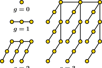
Figure 2: (Color online) Illustration for the growing process of a special network corresponding to $m=3$.

The networks considered here have some properties observed for many real networks. According to the construction process, at any new iteration, the degree of every old node increases by 1, independently of the node degrees. Thus, the degree distribution of the networks is exponential, instead of a power law [25]. On the other hand, the diameter (i.e., the maximum of shortest-path distance between all pair of nodes) of $U_{g}$ is $(2g-1)(m-1)$ that grows logarithmically with the network size, showing that the networks are of small-world [35]. Moreover, some other properties, e.g., the adjacency spectrum [28], can also be determined analytically.

3 Random walks on the networks

After introducing the family $U_{g}$ of networks and their properties, we will study the discrete random walks [27] performed on $U_{g}$. At each time step, the walker (particle) jumps uniformly (i.e., with the same probability) from its current position to any of its neighboring nodes. One of the most important quantities characterizing such a random walk is the FPT [12]. Let $F_{i,j}(g)$ denote the FPT for a walker, staring from node $i$ in $U_{g}$ to first arrive at node $j$. What we are concerned with is how the scalings of FPTs behave as the network size increases.

In the following, we will focus on three cases of random walks. Firstly, we will investigate a trapping issue, namely, random walks with a single immobile trap located at the initial node, and determine the MFPT to the initial node averaged over all nodes in $U_{g}$. Then, we will compute the MFPT from the initial node to another node selected uniformly from all nodes in $U_{g}$. Finally, we will determine the MFPT between all pairs of nodes in $U_{g}$.

3.1 MFPT from all other nodes to the initial node

First, we study a particular trapping problem on $U_{g}$, in which the single trap is positioned at the initial node. To facilitate computation, we introduce an alterative construction method for the networks, which highlights their self-similar architecture, as follows. Suppose one has $U_{g}$. The next iteration of the network, $U_{g+1}$, can be obtained by joining $m$ copies of $U_{g}$ in a way as illustrated by Fig. 3.

Figure 3: Another construction of the network. The networks after $g+1$ iterations, $U_{g+1}$, consist of $m$ replicas of $U_{g}$ denoted $U_{g}^{(1)}$, $U_{g}^{(2)}$, $U_{g}^{(3)}$, $\cdots$, and $U_{g}^{(m)}$, which are connected to each other by adding $m-1$ edges among the $m$ copies of the initial node.

For convenience of description, we label the initial node in $U_{g}$ as $1$, while the duplicates of initial nodes in $U_{g-1}^{(\eta)}(\eta=2,3,\ldots,m)$ are sequentially labeled as $2$, $3$, $\ldots$, $m$. In addition, let $T_{i}(g)$ be the FPT, $F_{i,1}(g)$, also called the trapping time, of node $i$ in $U_{g}$, which is the expected time for a walker starting from $i$ to first visit the trap node. Obviously, for all $g\geq 0$, $T_{1}(g)=0$. Let $T_{\rm tot}(g)$ express the total trapping times for all nodes in $U_{g}$, i.e.,

$$T_{\rm tot}(g)=\sum_{i\in U_{g}}T_{i}(g)\,.$$ (1)

Then, the MFPT, also called the mean trapping time (MTT) and denoted by $\langle T\rangle_{g}$, is the average of $T_{i}(g)$ over all starting nodes distributed uniformly in $U_{g}$, given by

$$\langle T\rangle_{g}=\frac{1}{N_{g}}\sum_{i\in U_{g}}T_{i}(g)=\frac{T_{\rm tot}(g)}{N_{g}}\,.$$ (2)

Thus, to obtain $\langle T\rangle_{g}$, one should first determine $T_{\rm tot}(g)$.

We first compute the FPTs, $F_{i+1,i}$ ($i=1,2,\ldots,m-1$) between two arbitrary copies of the initial node of $U_{g-1}$ that are directly connected to each other. Since $U_{g}$ has a treelike structure, according to the result obtained previously in [18, 36, 37], e.g., Eq. (2) in [18], we have

$$F_{i+1,i}(g)=2(m-i)m^{g-1}-1\,$$ (3)

for all $i\in[1,m-1]$, yielding

$$T_{\rm tot}(g) = T_{\rm tot}(g-1)+\sum_{\eta=2}^{m}\sum_{i\in U_{g-1}^{(\eta)}}T_{i}(g)$$ (4)

$$= mT_{\rm tot}(g-1)+\sum_{i=2}^{m}[N_{g-1}F_{i,1}(g)]\,.$$

Considering the treelike structure of $U_{g}$, we have

$$F_{i,1}(g)=F_{i,i-1}(g)+F_{i-1,i-2}(g)+\cdots+F_{3,2}(g)+F_{2,1}(g)\,.$$ (5)

Plugging Eqs. (3) and (5) into Eq. (4), we obtain

$$T_{\rm tot}(g)=mT_{\rm tot}(g-1)+\frac{1}{3}(2m^{2}-3m+1)m^{2g-1}-\frac{1}{2}(m-1)m^{g}\,.$$ (6)

With the initial condition $T_{\rm tot}(0)=0$, Eq. (6) is inductively solved, giving

$$T_{\rm tot}(g)=m^{2g}\left(\frac{2}{3}m-\frac{1}{3}\right)-m^{g}\left[\left(\frac{g}{2}+\frac{2}{3}\right)m-\left(\frac{g}{2}+\frac{1}{3}\right)\right].$$ (7)

Inserting Eq. (7) into Eq. (2), we obtain a closed-form expression for the MTT on network $U_{g}$, as

$$\langle T\rangle_{g}=m^{g}\left(\frac{2}{3}m-\frac{1}{3}\right)-\left(\frac{g}{2}+\frac{2}{3}\right)m+\left(\frac{g}{2}+\frac{1}{3}\right)\,.$$ (8)

Recalling $N_{g}=m^{g}$, we have $g=\ln N_{g}/\ln m$. Thus, $\langle T\rangle_{g}$ can be expressed in terms of the network size $N_{g}$ as

$$\langle T\rangle_{g}=\left(\frac{2}{3}m-\frac{1}{3}\right)N_{g}-\frac{\ln N_{g}}{2\ln m}(m-1)-\left(\frac{2}{3}m-\frac{1}{3}\right)\,.$$ (9)

Therefore, for large networks (i.e., $N_{g}\rightarrow\infty$),

$$\langle T\rangle_{g}\sim N_{g}\,,$$ (10)

implying that the MTT $\langle T\rangle_{g}$ increases linearly with the network size, independently of the degree of the initial node. This linear scaling is in sharp contrast to that of random exponential trees [23], in which the MTT depends on the degree of trapping node.

3.2 MFPT from the initial node to all other nodes

By definition, $F_{1,i}(g)$ denotes the FPT of the walker visiting node $i$ for the first time, assuming that the walker started at the initial node in $U_{g}$. Let $\langle H\rangle_{g}$ represent the mean value of $F_{1,i}(g)$ averaged over all target nodes $i$ in network $U_{g}$, called the partial mean first-passage time (PMFPT). Then, $\langle H\rangle_{g}$ is given by

$$\langle H\rangle_{g}=\frac{1}{N_{g}}\sum_{i\in U_{g}}F_{1,i}(g)\,.$$ (11)

Thus, the problem of finding $\langle H\rangle_{g}$ is reduced to determining the sum $\sum_{i\in U_{g}}F_{1,i}(g)$, denoted $H_{\rm{tot}}(g)$.

Unfortunately, the method for computing $T_{\rm{tot}}(g)$ is not suitable for $H_{\rm{tot}}(g)$. So, we seek for a feasible technique to derive $H_{\rm{tot}}(g)$. Below, we will apply the link between effective resistance and the FPTs for random walks [38, 39] to calculate $H_{\rm{tot}}(g)$ analytically. For this purpose, we replace each edge of $U_{g}$ by a unit resistor to obtain the corresponding resistor networks. To do so, let $R_{i,j}(g)$ represent the effective resistance between two nodes $i$ and $j$ of $U_{g}$. Then, we have [38, 39]: $F_{i,j}(g)+F_{j,i}(g)=2E_{g}R_{i,j}(g)$, which leads to

$$H_{\rm{tot}}(g)+T_{\rm{tot}}(g)=2E_{g}\sum_{i\in U_{g}}R_{1,i}(g)\,.$$ (12)

Equation (12) shows that if we have the sum $\sum_{i\in U_{g}}R_{1,i}(g)$ on the right-hand side, then we can easily obtain $H_{\rm{tot}}(g)$. Since, for any tree, the effective resistance $R_{i,j}(g)$ is equal to the geodesic distance $d_{i,j}(g)$ between $i$ and $j$, this makes it possible to determine the sum $\sum_{i\in U_{g}}R_{1,i}(g)$. To this end, we introduce a new quantity $d_{g}$, which is the sum of shortest distances between the initial node 1 and all other nodes in $U_{g}$. By definition, we have

$$d_{g}=\sum_{i\in U_{g}}d_{1,i}(g)\,.$$ (13)

Considering the self-similar network structure (see Fig. 3), we can easily obtain the recursion relation

$$d_{g}=m\,d_{g-1}+\frac{m(m-1)}{2}N_{g-1}\,.$$ (14)

Using $d_{1}=m(m-1)/2$, Eq. (14) is solved, giving

$$d_{g}=\frac{1}{2}g(m-1)m^{g}\,.$$ (15)

Then, we have

$$H_{\rm{tot}}(g) = 2E_{g}d_{g}-T_{\rm{tot}}(g)$$ (16)

$$= m^{2g}\left[g(m-1)-\frac{2}{3}m+\frac{1}{3}\right]-m^{g}\left(\frac{m-1}{2}g+\frac{2}{3}m-\frac{1}{3}\right)$$

and

$$\langle H\rangle_{g}=m^{g}\left[g(m-1)-\frac{2}{3}m+\frac{1}{3}\right]-\left(\frac{m-1}{2}g+\frac{2}{3}m-\frac{1}{3}\right)\,.$$ (17)

Equation (17) can be rewritten as a function of the network size $N_{g}$, as

$$\langle H\rangle_{g} = N_{g}\left[\frac{(m-1)\ln N_{g}}{\ln m}-\frac{2}{3}m+\frac{1}{3}\right]-\left[\frac{(m-1)\ln N_{g}}{2\ln m}+\frac{2}{3}m-\frac{1}{3}\right]\,.$$ (18)

Therefore, in the limit of the large network size $N_{g}$,

$$\langle H\rangle_{g}\sim N_{g}\ln N_{g}\,.$$ (19)

3.3 MFPT between all node pairs

In what follows, we will calculate the MFPT $\langle F\rangle_{g}$ among all node pairs in $U_{g}$, commonly called the global mean first-passage time (GMFPT) [40]. It should be noted that the GMFPT has been studied in [34]. Here we will derive an equivalent result using an approach different from but relatively easier than that in [34].

By definition, $\langle F\rangle_{g}$ is given by

$$\langle F\rangle_{g}=\frac{F_{\rm tot}(g)}{N_{g}(N_{g}-1)}=\frac{1}{N_{g}(N_{g}-1)}\sum_{i\neq j}^{N_{g}}\sum_{j=1}^{N_{g}}F_{i,j}(g)\,,$$ (20)

where the sum

$$F_{\rm tot}(g)=\sum_{i\neq j}^{N_{g}}\sum_{j=1}^{N_{g}}F_{i,j}(g)$$ (21)

denotes the sum of FPTs among all pairs of nodes. Hence, all that is left to find $\langle F\rangle_{g}$ is to determine $F_{\rm tot}(g)$.

According to the relation between FPTs and the effective resistance, we have

$$F_{\rm tot}(g)=E_{g}\,\sum_{i\neq j}^{N_{g}}\sum_{j=1}^{N_{g}}d_{i,j}(g)\,.$$ (22)

For brevity, we use $D_{g}$ to denote $\sum_{i\neq j}^{N_{g}}\sum_{j=1}^{N_{g}}d_{i,j}(g)$, which is the total geodesic distance among all pairs of nodes $U_{g}$.

Since $U_{g}$ can be obtained by the juxtaposition of $m$ copies of $U_{g-1}$ (i.e., $U_{g-1}^{(1)}$, $U_{g-1}^{(2)}$, $\cdots$, and $U_{g-1}^{(m)}$) at the edge nodes (replicas of the initial node in $U_{g-1}$), $D_{g}$ can be recast as

$$D_{g}=m\,D_{g-1}+\Delta_{g}\,,$$ (23)

where $\Delta_{g}$ is the sum over all shortest paths whose endpoints are not in the same copy of $U_{g-1}$.

Denote $\Delta_{g}^{\alpha,\beta}$ as the sum of all shortest paths with endpoints in $U_{g-1}^{\alpha}$ and $U_{g-1}^{\beta}$, respectively. According to the value of the distance between two edge nodes in $U_{g-1}^{\alpha}$ and $U_{g-1}^{\beta}$, we can partition the sum of path length $\Delta_{g}^{\alpha,\beta}$ into $m-1$ classes, denoted by $\Delta_{g}^{\alpha,\beta}(q)$ with $q=1,2,\ldots,m-1$ being the distance between the two boundary nodes in $U_{g-1}^{\alpha}$ and $U_{g-1}^{\beta}$. That is, $\Delta_{g}^{\alpha,\beta}=\sum_{q=1}^{m-1}\Delta_{g}^{\alpha,\beta}(q)$. It is easy to see that the number of elements in class $\Delta_{g}^{\alpha,\beta}(q)$ is $m-q$. On the other hand, any two elements belonging to $\Delta_{g}^{\alpha,\beta}(q)$ have an identical length of $4N_{g-1}d_{g-1}+2q(N_{g-1})^{2}$. Then, the total crossing path length $\Delta_{g}$ can be expressed as

$$D_{g}=m\,D_{g-1}+\sum_{q=1}^{m-1}(m-q)[4N_{g-1}d_{g-1}+2q(N_{g-1})^{2}]\,.$$ (24)

With the initial condition $D_{1}=m(m-1)(m+1)/3$, Eq. (24) is solved to yield

$$D_{g}=\frac{1}{3}m^{g}\left[(3g-2)m^{g+1}-(3g-1)m^{g}+2m-1\right]\,.$$ (25)

Using the above-obtained results, the expression for $\langle F\rangle_{g}$ reads

$$\langle F\rangle_{g} = \frac{E_{g}D_{g}}{N_{g}(N_{g}-1)}=\frac{D_{g}}{N_{g}}$$ (26)

$$= m^{g}\left[g(m-1)-\frac{2}{3}m+\frac{1}{3}\right]+\frac{2}{3}m-\frac{1}{3},$$

which can be rewritten in terms of $N_{g}$ in the following form:

$$\langle F\rangle_{g}=N_{g}\left[\frac{(m-1)\ln N_{g}}{\ln m}-\frac{2}{3}m+\frac{1}{3}\right]+\frac{2}{3}m-\frac{1}{3}\,,$$ (27)

consistent with the result previously obtained in [34].

Equation (27) uncovers the explicit dependence relation of $\langle F\rangle_{g}$ on the network size $N_{g}$ and the parameter $m$. In the case of $N_{g}\rightarrow\infty$, we have the following expression:

$$\langle F\rangle_{g}\sim N_{g}\ln N_{g}\,.$$ (28)

3.4 Analysis and comparison

Our results can be related to the efficiency of information transmission. Notice that if we consider the walker in the random-walk dynamics as an information messenger, then the $\langle T\rangle_{g}$ measures the efficiency of the initial node (as a receiver) in receiving information, while $\langle H\rangle_{g}$ shows how efficient of the initial node is as a sender to transmit information to other nodes, and $\langle F\rangle_{g}$ is the efficiency of information sending when the sender is distributed with equal probability among all nodes.

The above results, provided in Eqs. (10) and (19), show evidently that the dominant behaviors for $\langle T\rangle_{g}$ and $\langle H\rangle_{g}$ are different. The former follows $\langle T\rangle_{g}\sim N_{g}$, while the latter obeys $\langle H\rangle_{g}\sim N_{g}\,\ln N_{g}$, greater than the former. This means that the initial node is more efficient in receiving information than sending information. On the other hand, Equation (28) together with Eqs. (10) and (19) means that although the efficiency of the initial node in receiving information is higher than that of the average over other nodes, its ability of sending information is similar to the others. Equations (10), (19) and (28) also show that the linear scaling of the efficiency for the initial node measured by the MTT is not a representative property of the networks, but the $N_{g}\ln N_{g}$ behavior for the initial node sending information is so.

Our obtained results can be compared with those previously reported for other treelike networks. Equations (10) and (28) imply that the position of the trap significantly affects the scalings of the MTT for the trapping problem with a single trap. This behavior is similar to that in the small-world scale-free trees [24, 29], but is in contrast to that of trapping in the $T-$fractals [16, 18, 19] and the fractal scale-free trees [24], where the MTT does not depend on the trap location. In contrast, as shown in Eqs. (19) and (28), the initial node has the same dominant scaling of the PMFPT as that of the average of PMFPTs over all senders. This equality between PMFPT and GMFPT among all node pairs has also been observed for other trees, including the $T-$fractals [16, 18, 19] and fractal scale-free trees [24]. However, the scaling of PMFPT for different trees may have different behaviors.

In addition, the leading asymptotic $N_{g}\ln N_{g}$ dependence of GMFPT with the network size is also compared to the scalings found from other treelike networks with different degree distributions. In the standard fractal trees, such as the $T$-fractals [16, 18, 19] and the Vicsek fractals [21], the GMFPT $\langle F\rangle$ increases superlinearly with the network size $N$, which has also been observed from the family of scale-free trees with fractality [24]. For star graphs, the GMFPT $\langle F\rangle$ grows linearly with $N$ [21]; while for linear chains, $\langle F\rangle$ scales as a square root of $N$ [21]. However, for the class of scale-free small-world trees [24, 29], the GMFPT $\langle F\rangle$ also changes with $N$ as $\langle F\rangle\sim N\ln N$, which follows the same scaling as that of the exponential trees studied here.

Finally, combining the present work and the previous studies, it can be seen that random walks in trees display rich behaviors in the context of the FPT. At first sight, degree distribution is perhaps the root responsible for the rich phenomena. However, in [24], it was shown that the FPT in fractal and non-fractal scale-free networks may exhibit quite disparate scalings, meaning that degree distribution alone cannot determine the FPT for random walks on trees. We argue that the FPT on trees is determined by the short-path length from the resource node to the target node, while the impact of other structural properties is encoded in the short-path length, since the FPT $F_{ij}$ from an arbitrary node $i$ to $j$ is actually related to the FPTs of those node pairs for two directly connected nodes along the unique short-path direction to the target node, i.e., $F_{ij}=F_{ii_{1}}+F_{i_{1}i_{2}}+F_{i_{2}i_{3}}+\cdots+F_{i_{x}i_{y}}+F_{i_{y}j}$ provided that $i-i_{1}-i_{2}-i_{3}-\cdots-i_{x}-i_{y}-j$ is the shortest path from $i$ to $j$. For example, the FPT on the non-fractal treelike scale-free networks [24] and on the exponential networks studied here display similar behaviors, since both types of networks are of small world with the average distance increasing logarithmically in the network size, in spite of that they have distinct degree distributions. As another example, the FPT on some standard fractal trees (e.g. the $T$-fractals [18, 19] and the Vicsek fractals [21]) displays a superlinear dependence on the system size, which is also due to their average distance.

4 Conclusions

We have presented a detailed analysis of the simple random walks on a class of treelike small-world networks exhibiting an exponential degree distribution. We first investigated the trapping problem, focusing on a peculiar case with the trap fixed at the initial node, and obtained the exact solution to the MTT, the dominating scaling of which varies lineally with the network size $N$. We then studied the random walks staring from the initial node, and determined analytically the PMFPT from the initial node to all other nodes, whose dominant behavior scales with $N$ as $N\ln N$. Moreover, we determined explicitly the GMFPT among all node pairs and showed that the GMFPT also increases with $N$ approximately as $N\ln N$. We finally related our results in terms of information transmission by regarding the walker as an information messenger, and compared them with those previously reported results for other treelike networks with disparate topological properties. Our work provides new and useful insight into random-walk dynamics running on treelike networks, and could further deepen our understanding of random walks on a tree [40].

References

References

- [1] R. Albert and A.-L. Barabási, Rev. Mod. Phys. 74, 47 (2002).
- [2] M. E. J. Newman, SIAM Rev. 45, 167 (2003).
- [3] S. Boccaletti, V. Latora, Y. Moreno, M. Chavez, and D.-U. Hwanga, Phys. Rep. 424, 175 (2006).
- [4] S. N. Dorogovtsev, A. V. Goltsev and J. F. F. Mendes, Rev. Mod. Phys. 80, 1275 (2008).
- [5] P. Villas Boas, F. A. Rodrigues, G. Travieso, and L. Costa, J. Phys. A 41, 224005 (2008).
- [6] J. Shao, S. V. Buldyrev, R. Cohen, M. Kitsak, S. Havlin, and H. E. Stanley, EPL 84, 48004 (2008).
- [7] C. Castellano, V. Loreto, A. Barrat, F. Cecconi, and D. Parisi, Phys. Rev. E 71, 066107 (2005).
- [8] L. Dall’Asta, A. Baronchelli, A. Barrat, and V. Loreto, Phys. Rev. E 74, 036105 (2006).
- [9] P. Sibani and K. H. Hoffmann, Phys. Rev. Lett. 63, 2853 (1989).
- [10] G. Lois, J. Blawzdziewicz, and C. S. O Hern, Phys. Rev. E 81, 051907 (2010).
- [11] D. Fisher, Mach. Learn. 2, 139 (1987).
- [12] S. Redner, A Guide to First-Passage Processes (Cambridge University Press, Cambridge, England 2001).
- [13] S. Condamin, O. Bénichou, and M. Moreau, Phys. Rev. Lett. 95, 260601 (2005).
- [14] S. Condamin, O. Bénichou, V. Tejedor, R. Voituriez, and J. Klafter, Nature (London) 450, 77 (2007).
- [15] B. Kahng and S. Redner, J. Phys. A: Math. Gen. 22, 887 (1989).
- [16] E. Agliari, Phys. Rev. E 77, 011128 (2008).
- [17] C. P. Haynes and A. P. Roberts, Phys. Rev. E 78, 041111 (2008).
- [18] Y. Lin, B. Wu, and Z. Z. Zhang, Phys. Rev. E 82, 031140 (2010).
- [19] Z. Z. Zhang, Y. Lin, S. G. Zhou, B. Wu, and J. H. Guan, New J. Phys. 11, 103043 (2009).
- [20] T. Vicsek J. Phys. A 16, L647 (1983).
- [21] Z. Z. Zhang, B. Wu, H. J. Zhang, S. G. Zhou, J. H. Guan, and Z. G. Wang, Phys. Rev. E 81, 031118 (2010).
- [22] E. M. Bollt and D. ben-Avraham, New J. Phys. 7, 26 (2005).
- [23] A. Baronchelli, M. Catanzaro, and R. Pastor-Satorras, Phys. Rev. E 78, 011114 (2008).
- [24] Z. Z. Zhang, Y. Lin, and Y. J. Ma, J. Phys. A 44, 075102 (2011).
- [25] A.-L. Barabási and R. Albert, Science 286, 509 (1999).
- [26] L. A. N. Amaral, A. Scala, M. Barthélémy, H. E. Stanley, Proc. Natl. Acad. Sci. U.S.A. 97, 11149 (2000).
- [27] J. D. Noh and H. Rieger, Phys. Rev. Lett. 92, 118701 (2004).
- [28] L. Barriére, F. Comellas, C. Dalfó, and M. A. Fiol, Linear Multilinear Algebra 57, 695 (2009).
- [29] S. Jung, S. Kim, and B. Kahng, Phys. Rev. E 65, 056101 (2002).
- [30] S. N. Dorogovtsev, J. F. F. Mendes, and J. G. Oliveira, Phys. Rev. E 73, 056122 (2006).
- [31] L. Barriére, F. Comellas, C. Dalfó, and M. A. Fiol, Linear Algebra Appl. 428, 1499 (2008).
- [32] Y. Qi, Z. Z. Zhang, B. L. Ding, S. G. Zhou, and J. H. Guan, J. Phys. A 42, 165103 (2009).
- [33] Z. Z. Zhang, Y. Qi, S. G. Zhou, Y. Lin, and J. H. Guan, Phys. Rev. E, 80, 016104 (2009).
- [34] F. Comellas and A. Miralles, Phys. Rev. E 81, 061103 (2010).
- [35] D. J. Watts and H. Strogatz, Nature (London) 393, 440 (1998).
- [36] J. D. Noh and H. Rieger, Phys. Rev. E 69, 036111 (2004).
- [37] J. D. Noh and S.-W. Kim, J. Korean Phys. Soc. 48, S202 (2006).
- [38] A. K. Chandra, P. Raghavan, W. L. Ruzzo, and R. Smolensky, in Proceedings of the 21st Annual ACM Symposium on the Theory of Computing (ACM Press, New York, 1989), pp. 574-586.
- [39] P. Tetali, J. Theor. Probab. 4, 101 (1991).
- [40] V. Tejedor, O. Bénichou, and R. Voituriez, Phys. Rev. E 80, 065104(R) (2009).